Abstract
Cylinder-pressure-based control is a key enabler for advanced pre-mixed combustion concepts. In addition to guaranteeing robust and safe operation, it allows for cylinder pressure and heat release shaping. This requires fast control-oriented combustion models. Over the years, mean-value models have been proposed that can predict combustion metrics (e.g., gross indicated mean effective pressure (), or the crank angle where 50% of the total heat is released (CA50)) or models that predict the full in-cylinder pressure. However, these models are not able to capture cycle-to-cycle variations. The inclusion of the cycle-to-cycle variations is important in the control design for combustion concepts, like reactivity-controlled compression ignition, that can suffer from large cycle-to-cycle variations. In this study, the in-cylinder pressure and cycle-to-cycle variations are modelled using a data-based approach. The in-cylinder conditions and fuel settings are the inputs to the model. The model combines principal component decomposition and Gaussian process regression. A detailed study is performed on the effects of the different hyperparameters and kernel choices. The approach is applicable to any combustion concept, but is most valuable for advance combustion concepts with large cycle-to-cycle variation. The potential of the proposed approach is successfully demonstrated for a reactivity-controlled compression ignition engine running on diesel and E85. The average prediction error of the mean in-cylinder pressure over a complete combustion cycle is bar and of the corresponding mean cycle-to-cycle variation is bar2. This principal-component-decomposition-based approach is an important step towards in-cylinder pressure shaping. The use of Gaussian process regression provides important information on cycle-to-cycle variation and provides next-cycle control information on safety and performance criteria.
1. Introduction
Concerns about global warming have resulted in dramatic reduction targets for emissions from on-road applications. This has boosted interest in high-efficiency and low-carbon propulsion methods in the transportation sector. This has led to a trend towards electrification for personal mobility, but the go-to technology for heavy-duty applications has not yet been decided. High-efficiency and clean internal combustion engines together with sustainable fuels are expected to play a significant role in the future [1,2,3]. Advanced combustion concepts provide promising solutions to increase thermal efficiency. Concepts like homogeneous charge compression ignition, partial premixed combustion, and reactivity-controlled compression ignition (RCCI) have been proposed [4]. From these concepts, RCCI provides high thermal efficiency and fuel flexibility as well as controllability. RCCI uses a combination of a low- and high-reactivity fuels during combustion [5,6]. By changing the ratio between low- and high-reactivity fuels and their injection timing, it is possible to optimise combustion phasing, duration, and magnitude. However, continuous monitoring of the combustion process and regulation of this ratio and timing is required to guarantee robust and safe operation [7,8].
1.1. Control Challenges for Advanced Combustion Concepts
The introduced advanced combustion concepts rely on controlled auto-ignition of the in-cylinder mixture of air, residuals from previous combustion, and fuel. These concepts are sensitive to changes in operating conditions, such as intake temperature and intake air mixture. This can result in misfires as well as undesired large cyclic variations, which are associated with unstable combustion. Also, mechanical limits for safe operation can be violated. This can lead to engine damage.
Cylinder-pressure-based control (CPBC) is a key concept for guaranteeing safe and stable operation of these advanced combustion concepts [8]. Typically, the measured in-cylinder pressure is used in next-cycle combustion control strategies to minimise cyclic variations in key combustion metrics. Several CPBC strategies have already been proposed in the literature; an overview of applied combustion metrics and control approaches can be found in [9]. Traditionally, these methods aim to realise the desired engine load and combustion phasing by controlling gross indicated mean effective pressure () and the crank angle (CA) where 50% of the heat is released (CA50), respectively. Combustion is considered to be stable in case the cyclic variance in is below 5%. For engine safety, peak pressure () and peak pressure rise rate () are monitored.
Alternatively, CPBC opens the route to in-cylinder pressure and heat release shaping. More precisely, contrary to the traditional control of individual combustion metrics, this approach aims to control the entire in-cylinder pressure curve. Consequently, focus is on the realisation of ideal thermodynamic cycles, which are associated with maximal thermal efficiency [10]. This is a promising approach that can explicitly deal with in-cylinder-pressure-related safety constraints and that further enhances robustness of the controlled combustion process. However, for this approach, control development requires information of the entire pressure curve.
1.2. Control-Oriented Combustion Modelling
Models are becoming increasingly important in control development. In addition to their role as digital twins in simulations, they are used in control design, they can assist in control calibration, and they can be embedded in model-based controllers. In this work, we focus on the development of control-oriented models (COMs) for controller design and calibration. To support in-cylinder pressure shaping studies, the COM should describe the relevant combustion characteristics, including the relation between the in-cylinder mixture composition, intake manifold pressure, and temperature, as model inputs, and the full in-cylinder pressure curve. In case of advanced combustion concepts, a description of the cycle-to-cycle variations should also be available.
For the COMs, a distinction can be made between two types of models:
- Physics-based models, that use first-principle physical relations to capture combustion behaviour;
- Data-based models, that use black-box modelling methods, where measurements are used to create a mapping from input to output.
For combustion modelling, various models are found in the literature.
1.2.1. Physics-Based Combustion Models
To model important combustion metrics, e.g., or CA50, basic physics-based models have been proposed [11,12,13,14,15,16]. These models provide a deterministic and dynamic view of the relationship between actuation and combustion metrics without determining the full in-cylinder pressure. To add new combustion metrics these models should be extended with new descriptions to capture the behaviour of these new metrics. This can be time-consuming and reduces the flexibility of these models during combustion control development.
To model the full in-cylinder pressure, more complex first-principle models have been proposed. These include a multi-zone model [17] and a fluid dynamic model [18]. The complexity of these models results in computation times that exceed the combustion time. Therefore, they are not suited as COMs. A reduction in computation time is achieved by using static, data-driven, deterministic regression models to capture the behaviour of important combustion metrics.
1.2.2. Data-Based Combustion Models
Various data-based combustion modelling approaches have been introduced. For example, a Gaussian process regression (GPR) model to map in-cylinder conditions to combustion metrics [19]; a state-space model identified using data to model combustion phasing and peak pressure rise rate [20]; or a frequency response function method to determine cylinder-individual behaviour [21]. These models are made to only provide information on the modelled combustion metrics. Therefore, the model has to be extended to include other metrics.
Capturing the full in-cylinder pressure using data, principal component decomposition (PCD) models have been proposed. These models consist of a weighted sum of principal components, where the weights are modelled using regression methods. A deterministic neural network to capture the behaviour of the weights has been proposed [22]. To include cycle-to-cycle variations in the model, a GPR model to capture the behaviour of the weights has been proposed [23]. Alternatively, a method that uses double Wiebe functions to model the full in-cylinder pressure curve has been used [24]. The parameters of the double Wiebe function are determined using measurement data. A random forest machine learning approach is applied to describe the change in the mean behaviour and cycle-to-cycle behaviour of these parameters. However, determining these parameters from a measured in-cylinder pressure curve can be difficult.
The use of the PCD of the in-cylinder pressure has already been proposed in several control and detection methods. This decomposition was used as input to a virtual emission sensor [25]. They were able to predict the air-to-fuel ratio and emissions quite accurately. Also, this decomposition was used for knock detection and avoidance [26,27]. They used the decomposition to derive a measure of proximity to engine knocking. This decomposition was used as an alternative method to maximise the thermal efficiency [10]. They used the decomposition to derive a measure of the closeness of a measured in-cylinder pressure to an idealised thermodynamic cycle.
1.3. Research Objective and Main Contributions
In this study, we will extend the work of Vlaswinkel et al. [23] by giving an extensive analysis on (1) the comparison of different kernels in the GPR approach with regards to prediction quality of important combustion metrics; (2) understanding the effects of modelling a correlated process as an uncorrelated Gaussian process; (3) using a data set with a wide range of operating conditions to show the effectiveness of the model.
This work is organised as follows. In Section 2, an overview is given of the experimental setup and the data sets used. Section 3 describes the data-based combustion model, including cycle-to-cycle variation. A detailed analysis of the effect on different hyperparameters is presented in Section 4. The prediction quality of the combustion model is demonstrated and validated in Section 5.
2. Single-Cylinder Engine Test Bench
In this section, we will give a description of the setup and the data sets used. A discussion is provided on the chosen inputs to the model and how these are determined.
2.1. System Description
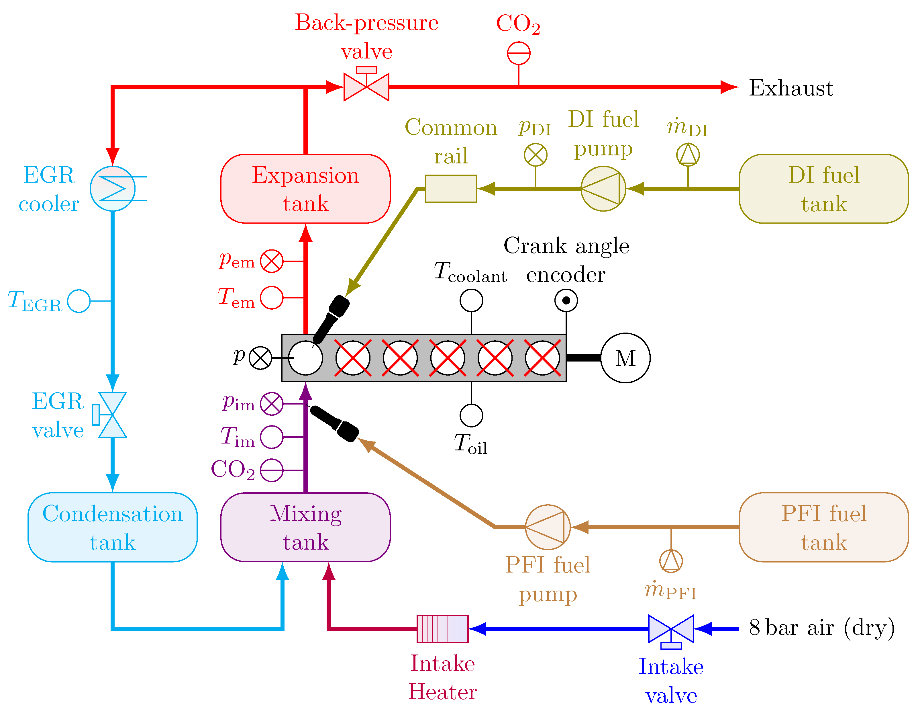
In this study, a modified PACCAR MX13 engine is used, as shown in Figure 1. Cylinders 2 to 6 have been removed and only cylinder 1 is operational. To keep the engine running at a constant speed, the electric motor of the engine dynamometer provides the required torque. The focus is on RCCI combustion with a single injection of diesel to autoignite the well-mixed charge of E85, air, and recirculated exhaust gas. The injection of diesel does not ignite the mixture, but the ignition is caused by the increased temperature as a result of cylinder compression. Therefore, there is a clear temporal separation between the injection of diesel and combustion. The direct injection (DI) of diesel is handled by a Delphi DFI21 injector connected to a common rail. The E85 port fuel injection (PFI) is handled by a Bosch EV14 injector fitted into the intake channel set at 5 bar. Both the DI and PFI fuel mass flows are measured using a Siemens Sitrans FC Mass 2100 Coriolis mass flow meter coupled with Mass 6000 signal converters. Boosted intake air is supplied at 8 bar and the pressure and temperature are regulated using a pressure regulator and an electric heater, respectively. The exhaust gas recirculation (EGR) fraction is regulated by the EGR and back-pressure butterfly valves. The EGR flow is cooled down to approximately room temperature by a cooled stream of process water. The condensation tank collects the condensation from the EGR flow and is drained regularly. The expansion and mixing tank are both attached to a surge tank to dampen pressure fluctuations in the intake and exhaust manifold as a result of single-cylinder operation. The in-cylinder pressure is sampled at 0.2° CA with a Kistler 6125C uncooled pressure transducer and amplified with a Kistler 5011B. A Leine Linde RSI 503 encoder provides crank angle information at a 0.2° interval. A Bronkhorst IN-FLOW F-106BI-AFD-02-V digital mass flow meter is used to measure the mass of the intake air flow. Pressures and temperatures located at different locations in the air path are measured every combustion cycle using a Gems Sensors & Controls 3500 Series pressure transmitter and Type-K thermocouples, respectively. The concentration of in the intake and exhaust flows are measured using an Horiba MEXA 7100 DEGR system. Table 1 lists the main specifications of the engine setup.
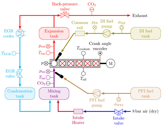
Figure 1.
Schematic of the single-cylinder PACCAR MX13 engine equipped with exhaust gas recirculation (EGR), direct injection (DI), and port fuel injection (PFI).

Table 1.
Main specifications of the engine setup.
2.2. Data Set for Model Training and Validation
The model relates in-cylinder conditions, determined at intake valve closing, to a resulting in-cylinder pressure. These conditions consist of a range of parameters related to engine speed, cylinder wall temperature, and mixture composition, pressure, and temperature. Since the engine is running at a single speed and at steady-state conditions the most relevant changes throughout the data set are a result of differences in mixture composition, pressure, and temperature. These can be described using intake and fuelling conditions. The chosen measurable parameters used to describe in-cylinder conditions are:
- Total injected energywhere and are the injected masses of PFI and DI fuels, and and are the lower heating values of the PFI and DI fuels;
- Energy-based blend ratio
- Start of injection of the directly injected fuel ;
- Pressure at the intake manifold ;
- Temperature at the intake manifold ;
- EGR ratiowith and the concentrations of as a fraction of the volume flow at the intake and exhaust, respectively.
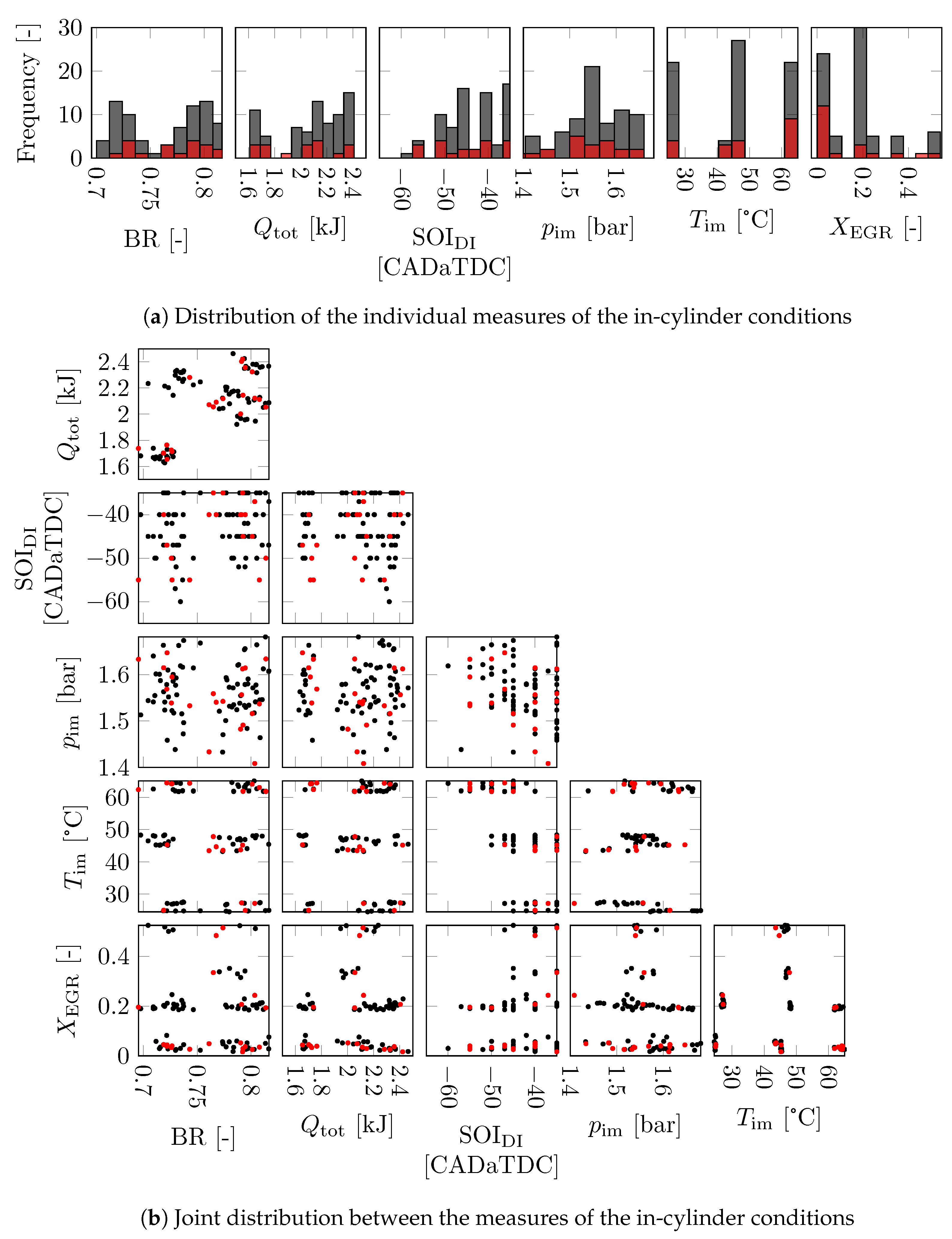
The variations in the in-cylinder conditions for the training data and validation data are shown in Figure 2. Figure 2a shows the distribution of each individual measure for the in-cylinder conditions. Figure 2b shows the joint distribution of the measures used for the in-cylinder conditions. The data set contains 95 different measurements consisting of consecutive cycles each. Both small and large cycle-to-cycle variations, and non-firing behaviour are present within the data set. In this work, each cycle is used and no averaging over the in-cylinder conditions and in-cylinder pressure traces in a measurement is performed before analysis. The data set is randomly divided into a training set of measurements and a validation set of the remaining measurements.
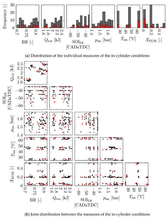
Figure 2.
Distribution of the in-cylinder conditions of the training (black) and validation data (red).
3. Combustion Model
In this section, the data-based approach to model the in-cylinder pressure is introduced. It is based on the method presented in Vlaswinkel et al. [23]. The approach combines principal component decomposition (PCD) and Gaussian process regression (GPR). To describe the in-cylinder pressure during the compression and power stroke, PCD is used to minimise the amount of information required by separating the influence of the in-cylinder conditions and the crank angle into two different mappings. GPR gives the possibility to model the in-cylinder pressure and cycle-to-cycle variation at different in-cylinder conditions. In Vlaswinkel et al. [23], the entire combustion cycle, including compression and expansion during motoring, is captured using the PCD/GPR method. In this study, the compression and expansion effects are separated from the effects of the actual combustion. The compression and expansion effects are modelled using adiabatic compression and expansion, while the effects of the actual combustion are modelled using the PCD/GPR method.
3.1. Principal Component Decomposition of the In-Cylinder Pressure
The in-cylinder pressure at crank angle , with the crank angle resolution, is decomposed as
where is a vector of weights and is the vector of principal components. In these vectors, the ith element is related to the ith principal component (PC). The in-cylinder condition is in the set containing all in-cylinder conditions present in the training set and the set spanning the modelled operation domain. It is assumed that the in-cylinder pressure during the intake stroke is equal to .
The PCs are computed using the eigenvalue method. The in-cylinder pressures contained in the training set are used. The vector is the ith unit eigenvector of the matrix , where , with the number of crank angle values. The elements in matrix P are defined as
such that the ath row of P contains the values of the in-cylinder pressure at the ath crank angle for all and the bth column of P contains the full in-cylinder pressure at all for the bth . The ith PC is defined as
The weight related to the ith PC is given by
where . The training set generates a single set of PCs. These PCs are ordered by relevance, where is the most relevant PC. The determination of the PCs and the required number of PCs will be considered later in this study.
3.2. Gaussian Process Regression to Capture Effects of In-Cylinder Conditions
GPR is used to estimate the behaviour of over the full operation domain . To include cycle-to-cycle variations, is described by a stochastic process as
with mean and variance . During this study, the correlation between the output variables and with , the number of PCs, will be neglected (i.e., is a diagonal matrix), since most of the literature on GPR assumes the output variables to be uncorrelated. This might affect the quality of the prediction of the cycle-to-cycle variation.
To improve the accuracy of prediction and the determination of hyperparameters, normalised in-cylinder conditions and weights will be used. Scaling the in-cylinder condition uses the mean and standard deviation of the jth in-cylinder condition variable over the full training set as
The scaling of the weights uses the mean and standard deviation of the ith in-cylinder conditions variable over the full training set as
Following [28], the scaled expected value and scaled covariance matrix without correlation can be computed as
and
where is the kernel and and are the kernel’s hyperparameters. The selection of both elements will be discussed in the next section.
To optimise the set of hyperparameters and found in the kernels, the marginal log-likelihood is maximised for each PC separately. The marginal log-likelihood is often used in determining the hyperparameters in GPR and does not depend on the kernel type. It is given by
where is a vector of the weights related to the ith PC at measured in the training set and .
Finally, the scaled expected value and scaled covariance matrix are descaled to complete the description of (8). The descaled expected value is given by
and the descaled covariance matrix is given by
3.3. Reconstructing the In-Cylinder Pressure with Cycle-to-Cycle Variation
The PCs (Section 3.1) and the estimate behaviour of (Section 3.2) can be combined to reconstruct a predicted in-cylinder pressure . Using (4), the mean and variance of the in-cylinder pressure can be described by
and
respectively.
4. Combustion Model Identification
The PCD and GPR require the selection of the number of PCs as well as the kernel type and hyperparameters. The training set is used to determine the PCs and values for the hyperparameters, while the validation set is used to determine the required amount of PCs and the best performing kernel type. For this selection, an assessment is made on the prediction accuracy of combustion metrics that are relevant for control [29]. To this end, the mean absolute error (MAE) is analysed, which is defined as
where is the number of validation measurements, and and are the combustion metrics resulting from the measured in-cylinder pressure and modelled in-cylinder pressure, respectively. The following combustion metrics are studied:
- gross indicated mean effective pressure,with displacement volume ;
- peak pressure, ;
- peak pressure rise rate, ;
- crank angle where 50% of the total heat is released,with the heat release given by [30]
- burn duration, , with CA75 and CA25 computed in a similar fashion to CA50;
- burn ratio,
4.1. Selection of Principal Components
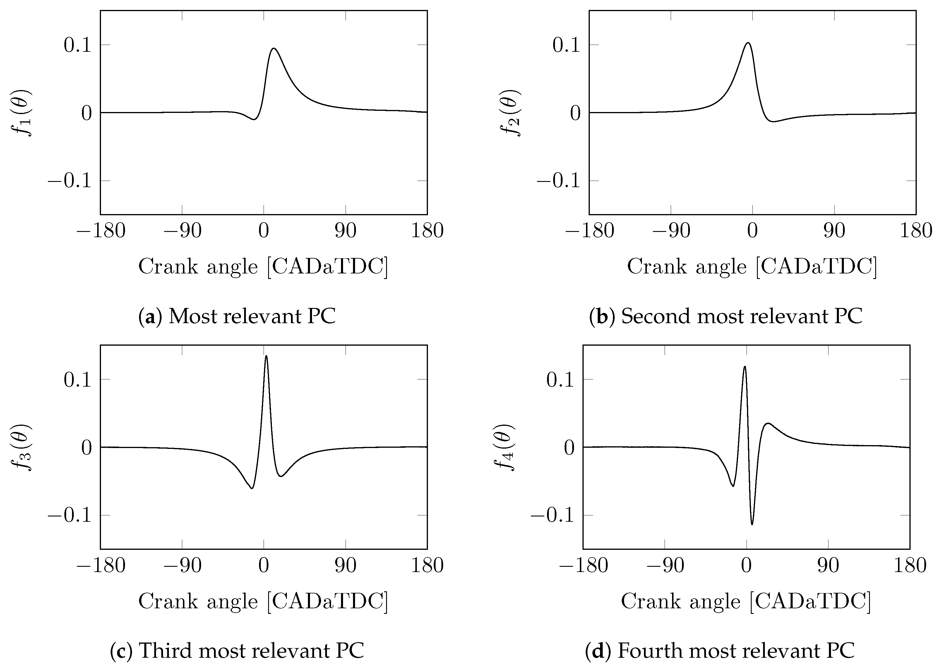
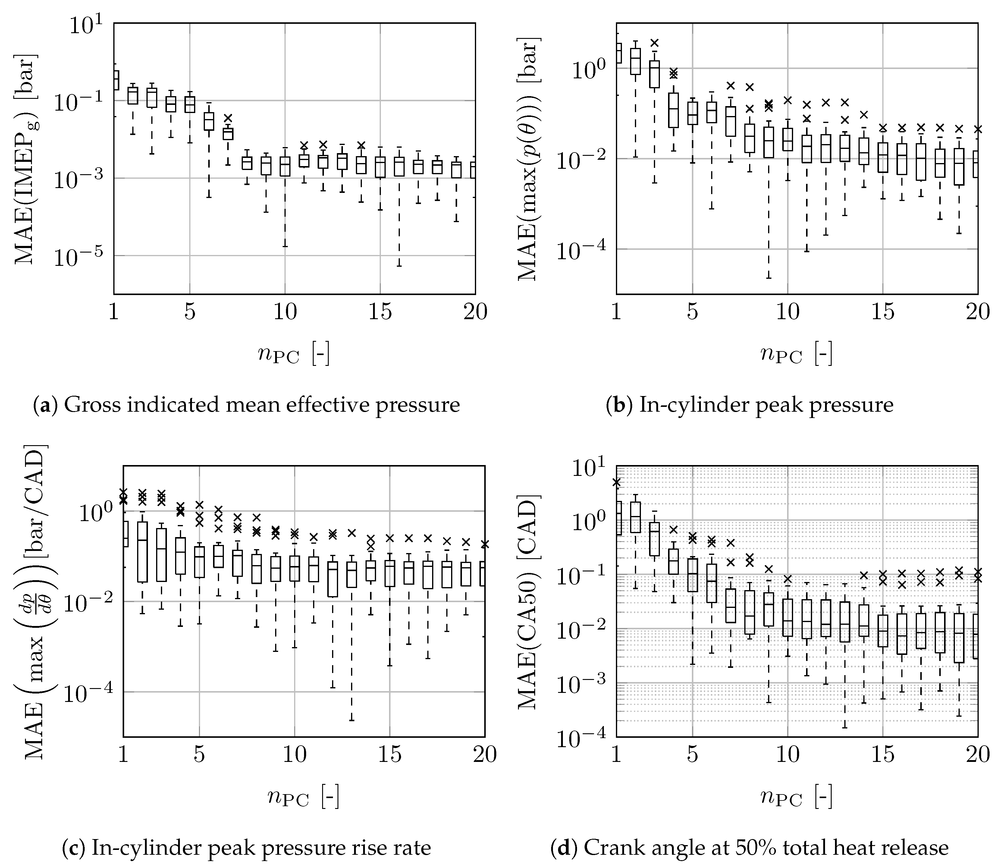
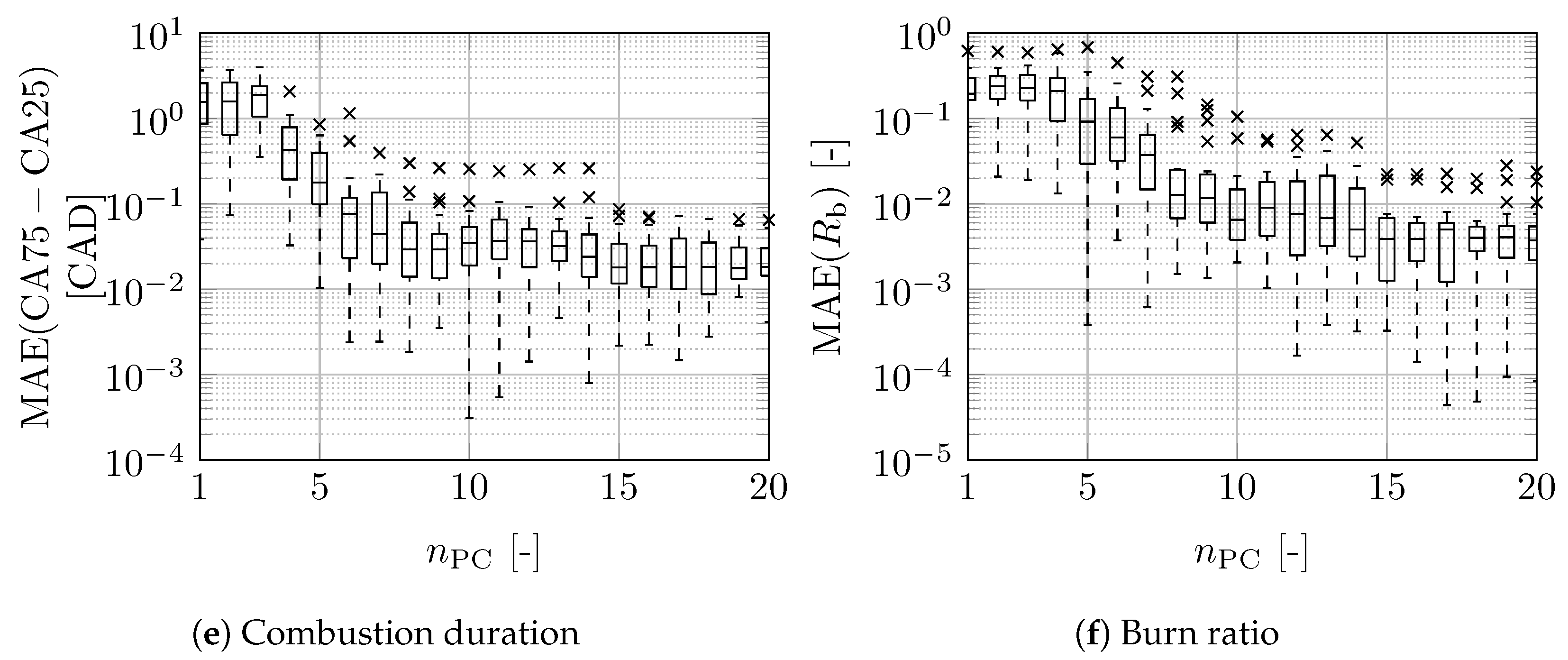
The first hyperparameter is the number of PCs . The GPR formulation proposed in Section 3.2 is not used in this part of the discussion. Figure 3 shows the four most relevant PCs derived from the training data, as discussed in Section 3.1. This figure illustrates that adding more PCs will add more higher-frequency components to the in-cylinder pressure. Figure 4 shows the absolute error in the corresponding combustion metrics by comparing measurements and model results. The modelled, decomposed in-cylinder pressure is based on an increasing number of PCs, using (6) to compute the required weights. Each measured cycle in the validation set is analysed separately. The figure indicates the minimum, maximum, median, and first and third quartiles, while the crosses show outliers. It can be seen that the largest gain in improvement is made at lower numbers of PCs. From the used training and validation sets, it is concluded that having more than eight PCs gives a negligible improvement. Therefore, is used in this study.
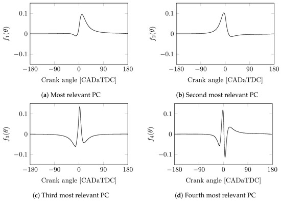
Figure 3.
Four most relevant principal components (PCs) resulting from the used training data.
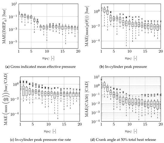

Figure 4.
Prediction error of combustion metrics for the validation data set using different numbers of principal components . The box plot shows the minimum, maximum, median, and first and third quartiles, while the crosses show outliers.
4.2. Selection of Kernel
Another important aspect in the quality of the model lies in the chosen kernel. This describes the correlation between all measured and predicted means and variance . The kernel types compared in this study rely on the distance measure
where and are scaled in-cylinder conditions. Each element of the kernel is computed individually. The elements of the kernels used in this work are:
- square exponential (SE):with the set of hyperparameters ;
- Matérn with :with the set of hyperparameters ;
- Matérn with :with the set of hyperparameters ;
- rational quadratic (RQ):with the set of hyperparameters .
For each kernel, a distinction is made between with and without automatic relevance determination (ARD). In the case where ARD is not used, the hyperparameter reduces to a scalar. In the case where ARD is used, the hyperparameter is a diagonal matrix with unique elements on the diagonal. The hyperparameters are determined by maximising the marginal log-likelihood, as described in (13), using the training set.
For the studied combustion metrics, Table 2 and Table 3 show the mean absolute error in the mean behaviour and in the standard deviation, respectively. For each combustion metric, the best result is in bold. In some cases, the difference between the best and second best option is negligible. The Matérn kernel with gives the best result for most of the combustion metrics in both mean behaviour and standard deviation for the data sets used. The resulting MAE of the mean-value behaviour shows a comparable or improved modelling error to those found in the literature, as illustrated in Table 4. Although the model accuracy of this work seems to be similar, the results have to be handled with care. It is difficult to give a fair comparison since most studies only give absolute errors and are unclear on the operating conditions.
Table 2.
Mean absolute error in the mean behaviour of key combustion metrics for the validation set using different kernels with . The best result for each combustion metric is in bold.
Table 3.
Mean absolute error in the standard deviation of key combustion metrics for the validation set using different kernels with . The best result for each combustion metric is in bold.
Table 4.
Comparison of the mean behaviour MAE of key combustion metrics between this work and studies in the literature [11,12,13,18,20,24]. The best result for each metric is in bold.
5. Validation of the Prediction Quality of the Combustion Model
The main goal of this work is to predict the in-cylinder pressure and cycle-to-cycle variation. In this section, the outcome of the model is compared to measurements using the validation data set. The hyperparameters shown in Table 5 are used. These choices for hyperparameters give the overall best prediction for the used data set, as discussed in Section 4.
Table 5.
Selected hyperparameters and kernel used during the validation in Section 5.
5.1. Overall Prediction Quality
First, the overall quality of the prediction is assessed. To evaluate the quality of the predicted in-cylinder pressure over a complete combustion cycle, the following measure is used for the mean behaviour:
and for cycle-to-cycle variation:
To assess the prediction quality of the combustion metrics, the observed average, minimum, and maximum relative differences between the predicted and measured combustion metrics are determined for the mean behaviour and cycle-to-cycle variation. In all metrics, a positive value is related to predicting higher values compared to the measured values.
The results are summarised in Table 6. For the validation set, the data-based combustion model is capable of accurately predicting the mean in-cylinder pressure curve: absolute errors are smaller than bar. The variance error is also small. Furthermore, this table shows that, except for , the mean behaviours have a good prediction quality (with a mean relative error up to −3.9%). According to the minimum and maximum relative difference, both over- and under-prediction are observed. Only the mean behaviour of shows a bad prediction quality and the model always under-predicts these values. This is expected, since peak pressure rise rates are difficult to predict; see also Figure 4. The prediction quality of the cycle-to-cycle variations can be improved, since most of the time the amount of cycle-to-cycle variation is over-predicted. Again, the worst performance is observed in .
Table 6.
Prediction quality of the full in-cylinder pressure (absolute error) and of the related combustion metrics (relative error) for the validation set.
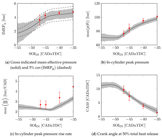
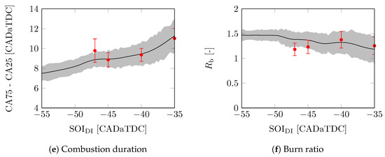
5.2. Variation in Start-of-Injection of Directly Injected Fuel
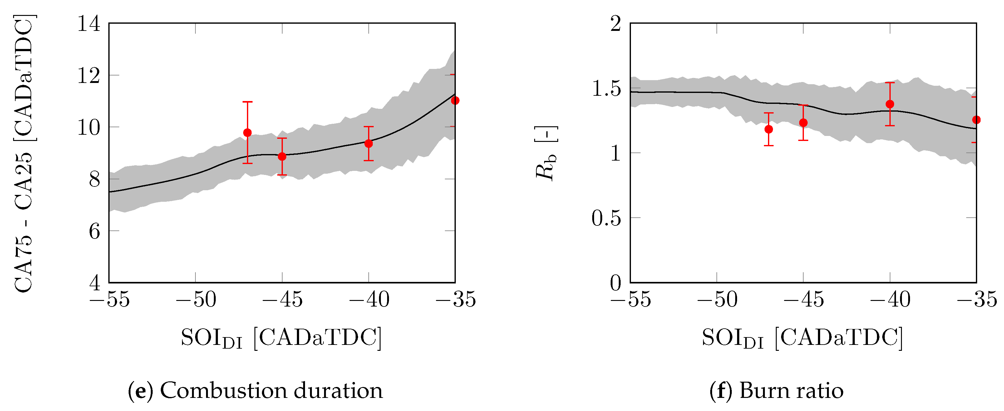
Figure 5 shows the modelled mean-value and cycle-to-cycle variations of important combustion parameters over a range of and the nominal conditions shown in Table 7. The results are in line with the results shown in Table 6. Except for the peak pressure rise rate, the mean value of the model is similar to that of the measurements. The modelled trend in the peak pressure rise rate seems to correspond to the measured values. The standard deviation of the model only matches with . The trend in the standard deviation of the model of and seems correct, but it is either too high or too low. The standard deviation of the model does not match the measurements for the , CA50, and .
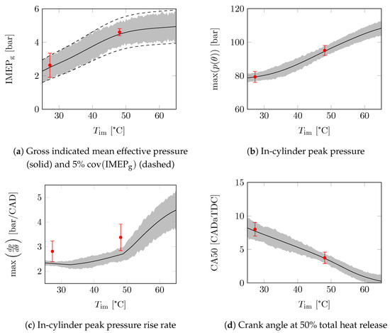
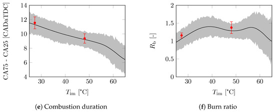
5.3. Variation in Intake Manifold Temperature
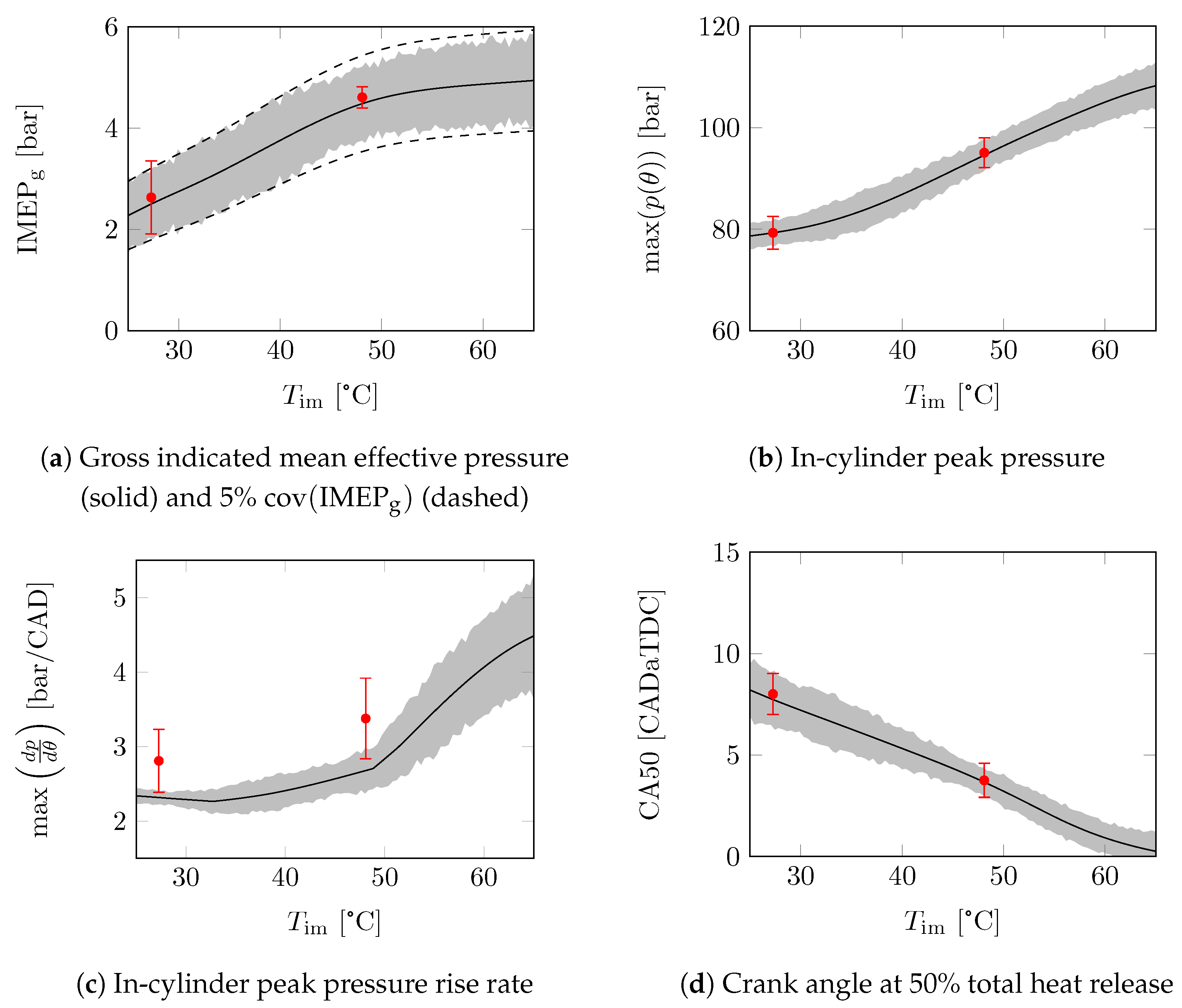
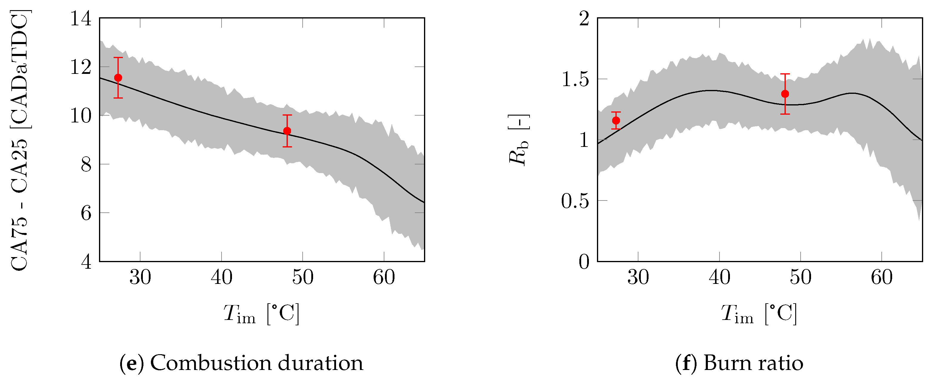
Figure 6 shows the modelled mean-value and cycle-to-cycle variations of important combustion parameters over a range of and the nominal conditions shown in Table 7. Again, the results are in line with the results shown in Table 6. Similarly to the sweep of , the mean value of the model is similar to that of the measurements except for the peak pressure rise rate. The modelled trend in the peak pressure rise rate seems to correspond the the measured values. The standard deviation of the model only matches with and CA50. The trend in the standard deviation of the model of seems correct, but it is too high. The standard deviation of the model does not match the measurements for the , , and .
5.4. Discussion on the GPR Modelling of Cycle-to-Cycle Variation
In both sweeps, the predicted standard deviations do not always match the measurements. In (8), , and are assumed to be independent to align with the available GPR literature; however, this independence is not necessarily the case. To evaluate the correlation between weights at a fixed , the Pearson correlation matrix R is used. This is given by
where and are the mean and standard deviation of the measured weights at , respectively. The values of R range from −1 to 1. When an element of R is zero, there is no correlation between the two variables. However, when an element is −1 or 1 there is full correlation between the two variables. The determinant of the R can be used as a measure for the amount of correlation, where ranges from 0 to 1. If all variables are fully uncorrelated. However, if at least two variables are fully correlated.
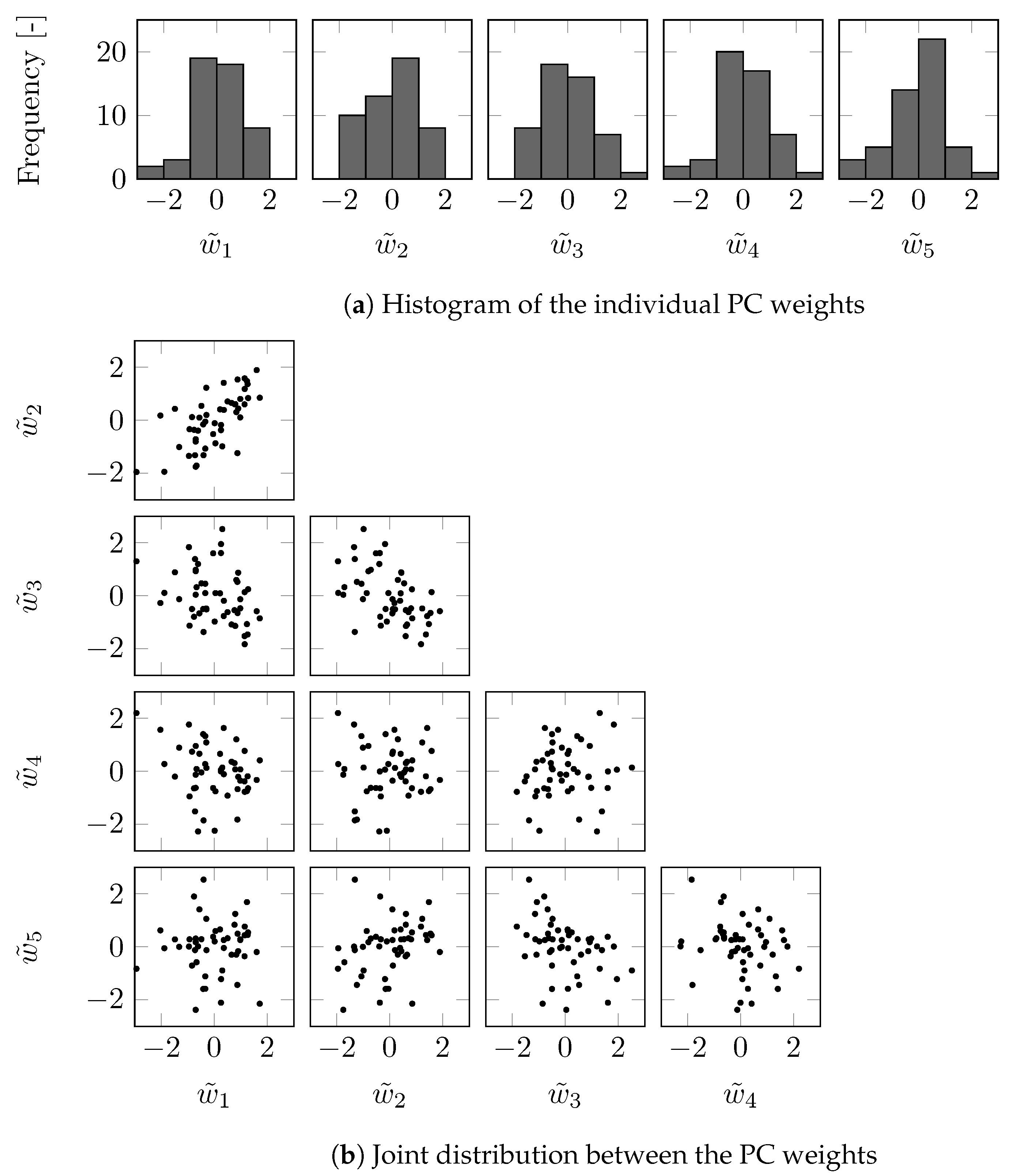
Figure 7 shows the distribution of the weights for 50 consecutive cycles of the first five PCs running at a constant with the least amount of coupling according to the determinant of the Pearson correlation matrix. In Figure 7, the weights have been scaled as
to emphasise the coupling. The corresponding symmetric Pearson correlation matrix is given by
with . This shows that the distributions between some of the weights are significantly correlated, as is also illustrated in Figure 7. Therefore, it is no surprise that the quality of the prediction of the cycle-to-cycle variation deviates from the proposed model. This emphasises the importance of developing GPR methods that include the correlation between the outputs.

Figure 7.
Distribution of the weights for cycles for the first five PCs for a constant with the least amount of coupling according to the Pearson correlation matrix.
6. Conclusions
In this study, a data-based model for the in-cylinder pressure and the corresponding cycle-to-cycle variations is proposed. This model combines a PCD of the in-cylinder pressure and GPR to map in-cylinder conditions and account for cyclic variations.
The proposed data-based modelling approach is successfully applied to an experimental RCCI engine setup. The assumption that the model can be split into a general principal component part and operating-condition-dependent weights is confirmed. A detailed analysis of the hyperparameters for the PCD and GPR is performed. It is found that, for the used data set, more than eight PCs do not further improve the accuracy of the decomposition based on important combustion metrics. For the GPR, the Matérn kernel with and without ARD gives the best results. The average prediction error of the mean in-cylinder pressure over a complete combustion cycle is bar and the corresponding mean cycle-to-cycle variation is bar2. The prediction quality of the mean behaviour of the evaluated combustion metrics has a relative inaccuracy ranging from −3.9% to 2.3%. The prediction error of the cycle-to-cycle variation of the evaluated combustion metrics ranges from 21.5% to 65.5%. The peak pressure rise rate is traditionally hard to predict; in the proposed model it has an inaccuracy of −22.7% in mean behaviour and −85.1% in cycle-to-cycle variation.
In the presented approach, the correlation between and has been neglected for ease of implementation. To improve the accuracy of the cycle-to-cycle variations, this correlation should be added. However, there are very few approaches that extend the GPR framework to including correlation between model outputs known in the literature.
In conclusion, the mean-value performance of our model is comparable or shows improvements compared to models found in the literature. This shows that, even when neglecting correlation, the model performs well. The model can be used for in-cylinder pressure shaping as proposed in Vlaswinkel and Willems [10]. Furthermore, it can be used in model-based optimisation approaches that take into account cycle-to-cycle variations and safety criteria. When combined with the PCD-based emission model of Henningsson et al. [25], the model provides a base for optimisation approaches with emission constraints.
Author Contributions
Conceptualisation, M.V. and F.W.; data curation, M.V.; formal analysis, M.V.; funding acquisition, F.W.; investigation, M.V.; methodology, M.V. and F.W.; project administration, F.W.; resources, F.W.; software, M.V.; supervision, F.W.; validation, M.V. and F.W.; visualisation, M.V.; writing—original draft, M.V.; writing—review and editing, M.V. and F.W. All authors have read and agreed to the published version of the manuscript.
Funding
The research presented in this study is financially supported by the Dutch Technology Foundation (STW) under project number 14927.
Data Availability Statement
The datasets presented in this article are not readily available because of agreements made for project funding. Requests to access the datasets should be directed to m.g.vlaswinkel@tue.nl.
Acknowledgments
The authors would like to thank Marnix Hage, Michel Cuijpers and Bart van Pinxten from the Zero Emission Lab at the Eindhoven University of Technology for their support during experimentation. The authors would like to thank Lucy Pao for proofreading this manuscript.
Conflicts of Interest
The authors declare no conflicts of interest.
References
- Leach, F.; Kalghatgi, G.; Stone, R.; Miles, P. The Scope for Improving the Efficiency and Environmental Impact of Internal Combustion Engines. Transp. Eng. 2020, 1, 100005. [Google Scholar] [CrossRef]
- Duarte Souza Alvarenga Santos, N.; Rückert Roso, V.; Teixeira Malaquias, A.C.; Coelho Baêta, J.G. Internal Combustion Engines and Biofuels: Examining Why This Robust Combination Should Not Be Ignored for Future Sustainable Transportation. Renew. Sustain. Energy Rev. 2021, 148, 111292. [Google Scholar] [CrossRef]
- Benajes, J.; García, A.; Monsalve-Serrano, J.; Guzmán-Mendoza, M. A Review on Low Carbon Fuels for Road Vehicles: The Good, the Bad and the Energy Potential for the Transport Sector. Fuel 2024, 361, 130647. [Google Scholar] [CrossRef]
- Dempsey, A.B.; Walker, N.R.; Gingrich, E.; Reitz, R.D. Comparison of Low Temperature Combustion Strategies for Advanced Compression Ignition Engines with a Focus on Controllability. Combust. Sci. Technol. 2014, 186, 210–241. [Google Scholar] [CrossRef]
- Kokjohn, S.L.; Hanson, R.M.; Splitter, D.A.; Reitz, R.D. Fuel Reactivity Controlled Compression Ignition (RCCI): A Pathway to Controlled High-Efficiency Clean Combustion. Int. J. Engine Res. 2011, 12, 209–226. [Google Scholar] [CrossRef]
- Reitz, R.D.; Duraisamy, G. Review of High Efficiency and Clean Reactivity Controlled Compression Ignition (RCCI) Combustion in Internal Combustion Engines. Prog. Energy Combust. Sci. 2015, 46, 12–71. [Google Scholar] [CrossRef]
- Li, J.; Yang, W.; Zhou, D. Review on the Management of RCCI Engines. Renew. Sustain. Energy Rev. 2017, 69, 65–79. [Google Scholar] [CrossRef]
- Paykani, A.; Garcia, A.; Shahbakhti, M.; Rahnama, P.; Reitz, R.D. Reactivity Controlled Compression Ignition Engine: Pathways towards Commercial Viability. Appl. Energy 2021, 282, 116174. [Google Scholar] [CrossRef]
- Willems, F. Is Cylinder Pressure-Based Control Required to Meet Future HD Legislation? IFAC-PapersOnLine 2018, 51, 111–118. [Google Scholar] [CrossRef]
- Vlaswinkel, M.; Willems, F. Cylinder Pressure Feedback Control for Ideal Thermodynamic Cycle Tracking: Towards Self-learning Engines. IFAC-PapersOnLine 2023, 56, 8260–8265. [Google Scholar] [CrossRef]
- Khodadadi Sadabadi, K.; Shahbakhti, M.; Bharath, A.N.; Reitz, R.D. Modeling of Combustion Phasing of a Reactivity-Controlled Compression Ignition Engine for Control Applications. Int. J. Engine Res. 2016, 17, 421–435. [Google Scholar] [CrossRef]
- Guardiola, C.; Pla, B.; Bares, P.; Barbier, A. A Combustion Phasing Control-Oriented Model Applied to an RCCI Engine. IFAC-PapersOnLine 2018, 51, 119–124. [Google Scholar] [CrossRef]
- Raut, A.; Irdmousa, B.K.; Shahbakhti, M. Dynamic Modeling and Model Predictive Control of an RCCI Engine. Control. Eng. Pract. 2018, 81, 129–144. [Google Scholar] [CrossRef]
- Sui, W.; González, J.P.; Hall, C.M. Combustion Phasing Modelling of Dual Fuel Engines. IFAC-PapersOnLine 2018, 51, 319–324. [Google Scholar] [CrossRef]
- Irdmousa, B.K.; Rizvi, S.Z.; Veini, J.M.; Nabert, J.D.; Shahbakhti, M. Data-Driven Modeling and Predictive Control of Combustion Phasing for RCCI Engines. In Proceedings of the 2019 American Control Conference (ACC), Philadelphia, PA, USA, 10–12 July 2019; pp. 1617–1622. [Google Scholar] [CrossRef]
- Kakoee, A.; Bakhshan, Y.; Barbier, A.; Bares, P.; Guardiola, C. Modeling Combustion Timing in an RCCI Engine by Means of a Control Oriented Model. Control Eng. Pract. 2020, 97, 104321. [Google Scholar] [CrossRef]
- Bekdemir, C.; Baert, R.; Willems, F.; Somers, B. Towards Control-Oriented Modeling of Natural Gas-Diesel RCCI Combustion. In Proceedings of the SAE 2015 World Congress & Exhibition, London, UK, 21 April 2015. [Google Scholar] [CrossRef]
- Klos, D.; Kokjohn, S.L. Investigation of the Sources of Combustion Instability in Low-Temperature Combustion Engines Using Response Surface Models. Int. J. Engine Res. 2015, 16, 419–440. [Google Scholar] [CrossRef]
- Xia, L.; de Jager, B.; Donkers, T.; Willems, F. Robust Constrained Optimization for RCCI Engines Using Nested Penalized Particle Swarm. Control. Eng. Pract. 2020, 99, 104411. [Google Scholar] [CrossRef]
- Basina, L.N.A.; Irdmousa, B.K.; Velni, J.M.; Borhan, H.; Naber, J.D.; Shahbakhti, M. Data-Driven Modeling and Predictive Control of Maximum Pressure Rise Rate in RCCI Engines. In Proceedings of the 2020 IEEE Conference on Control Technology and Applications (CCTA), Montreal, QC, Canada, 24–26 August 2020; pp. 94–99. [Google Scholar] [CrossRef]
- Verhaegh, J.; Kupper, F.; Willems, F. Data-Driven Air-Fuel Path Control Design for Robust RCCI Engine Operation. Energies 2022, 15, 2018. [Google Scholar] [CrossRef]
- Pan, W.; Korkmaz, M.; Beeckmann, J.; Pitsch, H. Unsupervised Learning and Nonlinear Identification for In-Cylinder Pressure Prediction of Diesel Combustion Rate Shaping Process. In Proceedings of the 13th IFAC Workshop on Adaptive and Learning Control Systems ALCOS, Winchester, UK, 4–6 December 2019; Volume 52, pp. 199–203. [Google Scholar] [CrossRef]
- Vlaswinkel, M.; De Jager, B.; Willems, F. Data-Based In-Cylinder Pressure Model Including Cyclic Variations of an RCCI Engine. IFAC-PapersOnLine 2022, 55, 13–18. [Google Scholar] [CrossRef]
- Mishra, C.; Subbarao, P. Design, Development and Testing a Hybrid Control Model for RCCI Engine Using Double Wiebe Function and Random Forest Machine Learning. Control Eng. Pract. 2021, 113, 104857. [Google Scholar] [CrossRef]
- Henningsson, M.; Tunestål, P.; Johansson, R. A Virtual Sensor for Predicting Diesel Engine Emissions from Cylinder Pressure Data. IFAC Proc. Vol. 2012, 45, 424–431. [Google Scholar] [CrossRef]
- Panzani, G.; Ostman, F.; Onder, C.H. Engine Knock Margin Estimation Using In-Cylinder Pressure Measurements. IEEE/ASME Trans. Mechatron. 2017, 22, 301–311. [Google Scholar] [CrossRef]
- Panzani, G.; Pozzato, G.; Savaresi, S.M.; Rösgren, J.; Onder, C.H. Engine Knock Detection: An Eigenpressure Approach. IFAC-PapersOnLine 2019, 52, 267–272. [Google Scholar] [CrossRef]
- Rasmussen, C.E.; Williams, C.K.I. Gaussian Processes for Machine Learning; The MIT Press: Cambridge, MA, USA, 2005. [Google Scholar] [CrossRef]
- Eriksson, L.; Thomasson, A. Cylinder State Estimation from Measured Cylinder Pressure Traces—A Survey * This Project Was Financed by the VINNOVA Industry Excellence Center LINK-SIC. IFAC-PapersOnLine 2017, 50, 11029–11039. [Google Scholar] [CrossRef]
- Wilhelmsson, C.; Tunestål, P.; Johansson, B. Model Based Engine Control Using ASICs: A Virtual Heat Release Sensor; Institut Francais du Petrole: Rueil-Malmaison, France, 2006. [Google Scholar]

Disclaimer/Publisher’s Note: The statements, opinions and data contained in all publications are solely those of the individual author(s) and contributor(s) and not of MDPI and/or the editor(s). MDPI and/or the editor(s) disclaim responsibility for any injury to people or property resulting from any ideas, methods, instructions or products referred to in the content. |
© 2024 by the authors. Licensee MDPI, Basel, Switzerland. This article is an open access article distributed under the terms and conditions of the Creative Commons Attribution (CC BY) license (https://creativecommons.org/licenses/by/4.0/).