Abstract
We evaluate the temporal complementarity in daily averages between wind and solar power potential in Chile using Spearman’s correlation coefficient. We used hourly wind speed and solar radiation data for 176 geographic points from 2004 to 2016. The results allow us to identify four zones: Zone A1 on the coast and in the valleys in the north of Chile between latitudes 18° S and 36° S, with moderate positive correlation; Zone A2 in the north Andes between latitudes 25° S and 33° S, with weak negative correlation; Zone B in the center-south part of the country between latitudes 36° S and 51° S with moderate negative correlation; and Zone C in the south, between latitudes 51° S and 55° S with null or weak positive correlation. On the one hand, the interannual analysis shows that Zone A1 keeps uniform correlation values with negative asymmetry, i.e., higher correlation values. On the other hand, there is positive asymmetry in most of the years in Zone A2, i.e., lower (or negative) values of correlation. Zone B shows an interannual oscillation of the median correlation, while Zone C shows a larger dispersion in the interannual results. Significance analysis shows that 163 out of the 176 points are statistically significant, while Zones A1, A2, and B have significant correlations, with Zone C being marginally significant. The results obtained are relevant information for further studies on the location of hybrid generation facilities. We expect our methodology to be instrumental in Chile’s energetic transition to a 100% renewable generation matrix.
1. Introduction and Literature Review
There is abundant empirical evidence that shows the increase in mean global temperature on our planet is attributed mainly to the emission of greenhouse effect gases (GEGs) and is significantly caused by human activities, such as the combustion of fossil fuels [1]. Because of this, multiple countries have signed the Paris Agreement [2], committing to modify their electric energy generation matrices. This change aims to transition towards more sustainable and less polluting energy sources to mitigate the impact of climate change, together with meeting the emission reduction global goals.
The current trend in energy transition is moving from fossil fuels to renewable energy sources, such as photovoltaic solar and wind. This trend has been pushed forward by the constant reduction in the costs of renewable technologies, the expansion of energy markets, and the development of public policies promoting the transformation in the energy generation sector. It has been estimated that following the global policies, a 7.5 gigaton reduction of equivalent CO2 will be achieved by 2030, according to the latest update on the roadmap to achieve net-zero emissions [3]. The change towards solar and wind energy is expected to account for 5 Gt.
Chile, as a country, has the goal of having a completely renewable electric energy generation matrix by 2030. By this time, all the thermoelectric plants using coal are expected to have ceased operation. The country aims to duplicate the current variable renewable energy (VRE) generation capacity, such as photovoltaic solar and wind, from 12 gigawatts (GW) to 24 GW by 2030, being about 55% of the total projected installed capacity [4]. Given the variable nature of solar and wind sources, a significant increase in the storage capacity is expected, reaching about 13.2 GW by 2026. This increase will focus on using battery-based energy storage (BBES) in northern Chile.
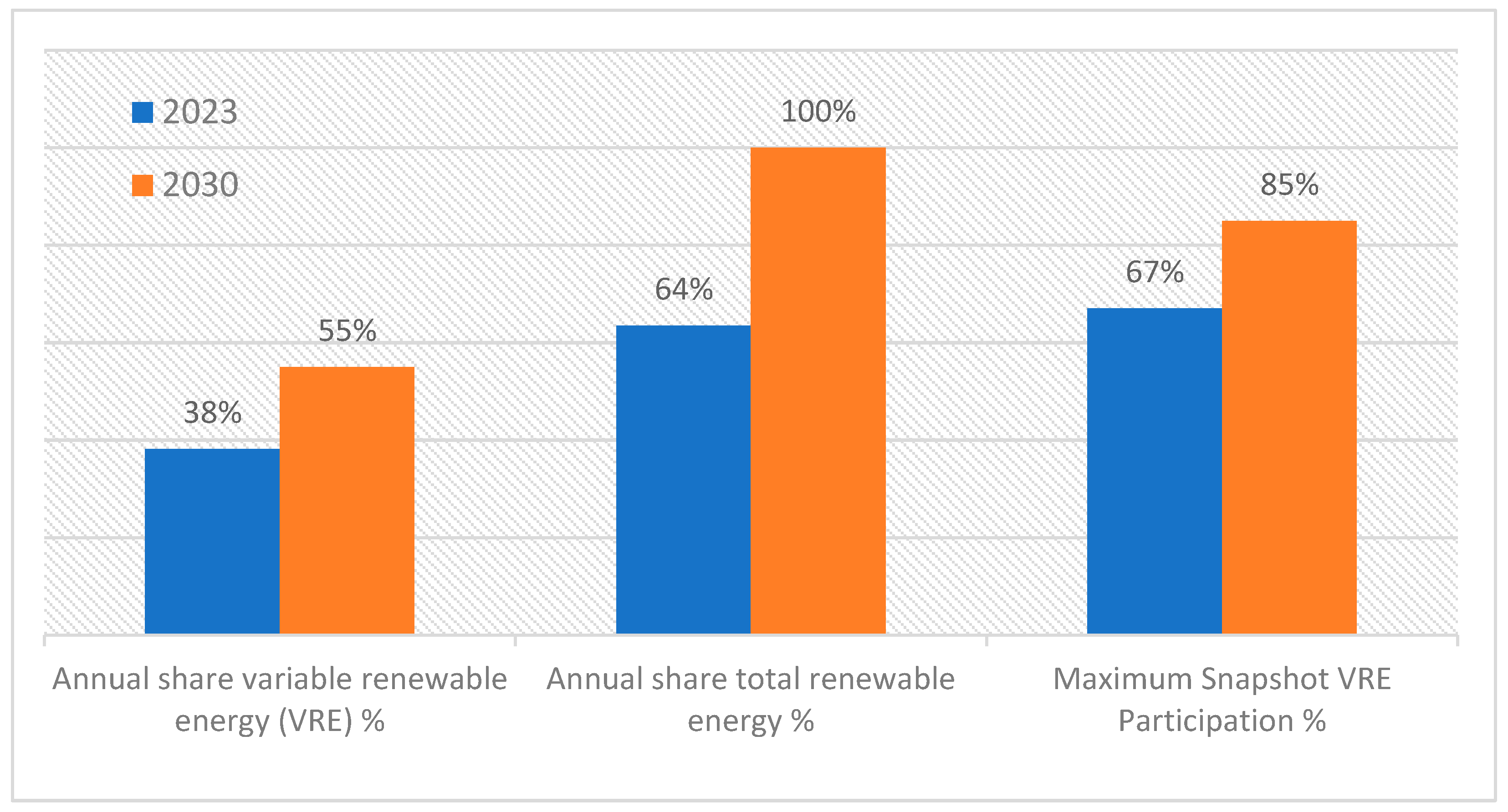
Table 1 shows the current electric energy installed generation capacity for the central electric system in Chile, the “Sistema Eléctrico Nacional (SEN)”. Variable renewable energy (VRE) sources of solar photovoltaic and wind have about 25.2% and 13% shares, respectively [5]. It is expected that VRE will increase its share up to 55% by 2030, and the total share of renewable energy sources will increase from 63.5% to 100% in the same timespan [4], as Figure 1 shows.

Table 1.
Installed electric energy generation capacity, Sistema Eléctrico Nacional (SEN), 2023.

Figure 1.
Renewable energy projection for Sistema Eléctrico Nacional (SEN), data from [4].
Most of the production in Chile is devoted to mining. Chile is the world’s largest copper producer and the second largest for lithium. The transition to renewable energy sources would decrease the uncertainty in the supply by decreasing the dependence on fossil energy sources, which Chile must import. Furthermore, from the environmental perspective, this energy transition will allow Chile to reduce its carbon footprint, contributing to reducing the emission of greenhouse effect gases.
The transition towards a 100% renewable electric generation matrix with a high share of VRE implies challenges that must solved. In the energy sector, generation must meet the demand at every moment, and energy cannot be stored on a large scale. Both photovoltaic and wind sources are by nature variable and are known to have non-manageable generation. The geographical concentration of VRE plants to take advantage of solar and wind potentials generates congestion in the transmission systems. This congestion creates energy dumping and distortions in the price of energy, causing disinterest in new-generation investments [6].
Multiple alternatives to mitigate the problems of using VRE in the generation matrix have been proposed, mainly oriented to the demand, i.e., changing the users’ behavior, and the offer, i.e., generation.
1.1. Demand
Demand can be satisfied by augmenting energy efficiency to avoid expanding the generation capacity of the VREs. In 2021, the Chilean Energy Minister created a Law and National Plan for Energy Efficiency to reduce the energy intensity by 10% by 2030. The plan considers residential energy efficiency, labeling electric devices according to efficiency, and increasing efficiency in buildings, transport, and productive sectors [7]. Outside Chile, the report “The evolution of energy efficiency policy to support clean energy transitions” from [8] indicates that energy efficiency is the first step towards a renewable electric energy generation matrix that reduces the emission of greenhouse effect gases, increases the energy security and decreases the energy consumption costs. Another way to influence users is to adjust the generation demand curve (offer curve) through pricing. This strategy implies the implementation of a smart grid in the system and modifying the electric market. A relevant example of this is the model proposed by the Arabic government of using intelligent energy, (tele)communication, and intelligent information systems, considering projects oriented to innovation, the development of human resources, and industrial viability [9].
1.2. Offer
From the point of view of the offer, there is also a set of solutions to meet the demand, considering the generation variability of VRE. We highlight the following:
1.2.1. Increase in the VRE Generation Capacity
The generation variability can be decreased by increasing the photovoltaic and wind generation to cover the demand peaks or storing the over-generation for later use. Ref. [10] indicates, for the Australian electric market, that the decrease in the costs of photovoltaic and wind electric generation technologies allows 100% renewable generation systems to be economically viable. To meet the demand, the installed capacity must be four times the demand if no energy storage is considered, reducing the current generation cost by 28% or if energy storage is considered by 55%, compared with the current prices.
1.2.2. Increase in Storage Capacity
Adding storage using different technologies and autonomy scales implies increased investment costs. Still, it is a way to solve the VRE generation variability problem. An alternative solution is deploying energy storage systems shared by multiple renewable energy sources in different locations. Ref. [11] argues that this strategy may reduce infrastructure costs while enabling a high penetration of renewable energy sources in the system. In [12], the authors conclude that energy storage is crucial for transforming the energy matrix toward renewable energy sources for the Spanish generation system. They suggest green hydrogen as a possible technology for energy storage towards a 100% renewable generation matrix.
1.2.3. Efficiency Improvements in VRE Generation
The increase in efficiency of photovoltaic panels and wind turbines implies a larger electric energy generation for the same installed capacity. The efficiency of a photovoltaic panel depends on parameters such as dust, reflection, inclination angle, orientation, shadows, radiation, and temperature. Such efficiency is around 6% and 20%. Recent studies point out that one of the parameters that affect the efficiency of photovoltaic panels the most is temperature, depending on the kind of cooling added to the panel [13].
1.2.4. Distributed Hybrid Generation
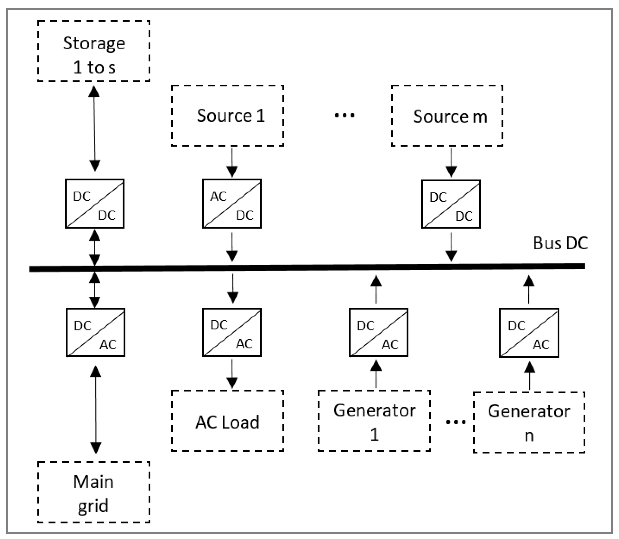
Its configuration uses two or more energy generation sources and one or more storage energy systems located in the same geographical location, with the ability to generate and consume energy. Figure 2 shows a distributed hybrid generation configuration (HRES) with “s” storage systems, probably of different kinds, such as lead–acid, lithium, green hydrogen batteries, etc. The system receives energy from “m” resources, either solar, wind, hydro, etc. [14]. The systems also receive energy from “n” diesel or other fuel generators. Finally, the energy supplied is used to serve the demand, where the excess energy is either stored or sent to a central system, which may also provide energy to this configuration.
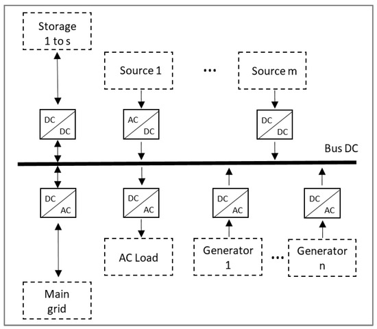
Figure 2.
A distributed hybrid generation configuration. Figure adapted from [14].
When a hybrid generation system is not connected to a central system, it is denoted as an isolated hybrid generation system, requiring storage if the energy source is a VRE. Distributed generation has several advantages, compared with a centralized system, because generation may be closer to the consumption points, reducing the transmission losses, favoring the use of VRE, and thus reducing the emission of greenhouse effect gases. The resulting configuration is named a hybrid renewable energy system (HRES) if the sources are renewable. Distributed hybrid generation may improve the system’s performance in meeting the demand compared to a centralized generation system when sources are VRE sources.
There are numerous studies on optimizing HRESs in terms of these systems’ design, scheduling, and operation. For example, ref. [15] presents an algorithm to optimize the design of an HRES with photovoltaic panels, wind turbines, diesel generators, and a battery energy storage system (BESS) to minimize the net present cost (NPC). It considers the renewable fraction index, the probability of energy supply interruption, and availability. The algorithm obtains a levelized cost of energy (LCOE) of 0.213 $/kWh, concluding on the role of storage as a management tool and the importance of the synergy between photovoltaic and wind systems. The authors of [16] present a multicriteria model for a hybrid system with photovoltaics, wind, and batteries connected to the network, considering the components’ costs, buying energy from the network, and CO2 emissions. They consider a reliability constraint in terms of the probability of unsupplied energy. To solve the model, they use an artificial electric field algorithm that designs the components of the HRES. They compare two scenarios, connected and disconnected from the electric network, finding that the connected design achieves between 7% and 10% more reliability. The authors of [17] show a complete review of the state-of-the-art optimal sizing of an HRES, considering the components, parameters, and methods used. They conclude that sizing an HRES requires using multiple objectives, such as reliability, costs, and emissions. They also note that using metaheuristics is more efficient than other approaches.
1.2.5. Energy Sources’ Complementarity
The degree of association between two or more energy resources is their complementarity. Suppose the energy resource availability is variable in time, such as in wind and solar energy. In that case, it is essential to quantify this relationship to make proper decisions to meet the demand required by the system. In general terms, the resources being in the same geographic region is denoted as temporal complementarity, and if not, as spatial complementarity.
Ref. [18] presents different ways to quantify the complementarity through metrics (Pearson’s correlation coefficient, Spearman’s and Kendall’s range correlation coefficients, autocorrelation, cross-correlation, etc.) and indices (of complementarity through wavelets, temporal complementarity index, etc.) Other authors [19] review different methodologies, techniques, and wind and solar datasets to evaluate complementarity. After they analyzed different metrics and indices, they concluded that there is neither a unique standard nor a common methodology for assessing energy complementarity.
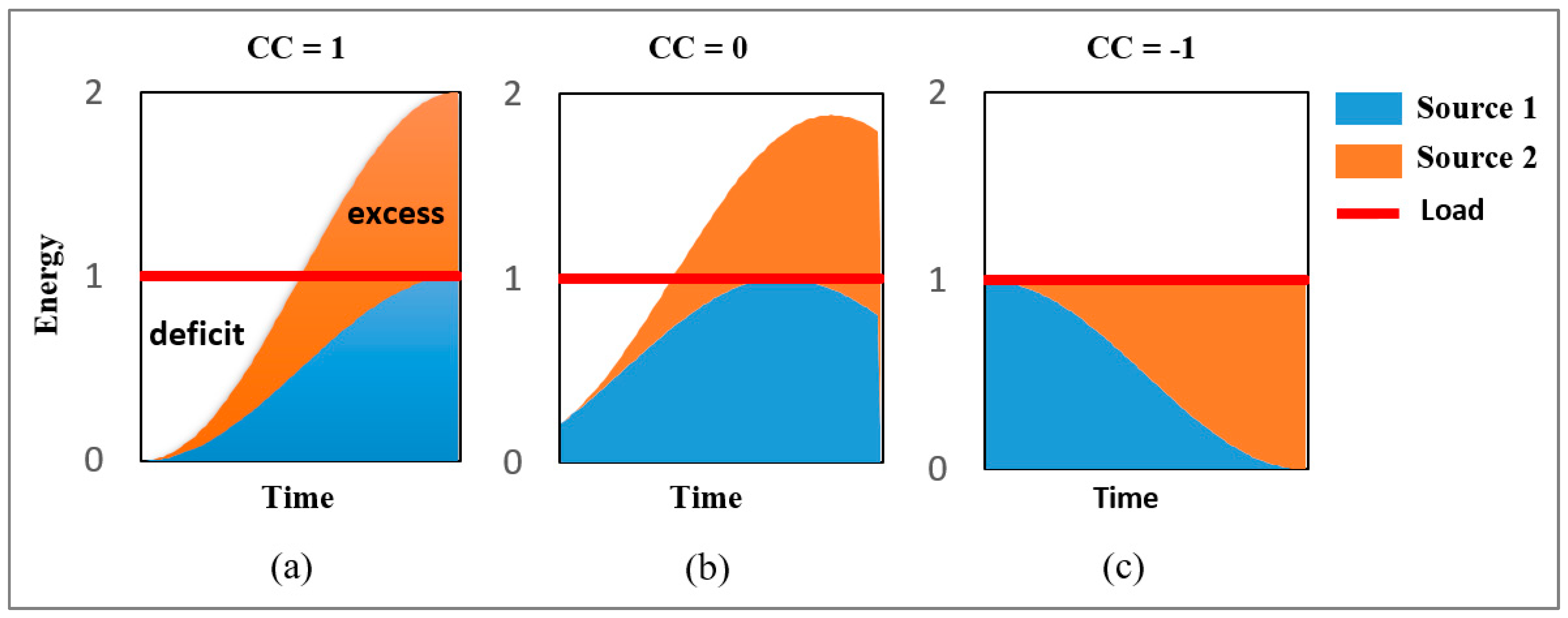
Figure 3 explains the concept of correlation coefficients for two resources whose availability is variable in time in three different scenarios. In scenario (a), both resources have unit correlation (CC = 1), meaning that the resources increase and decrease simultaneously and have their extremes simultaneously. In this scenario, there will be periods with energy deficit and surplus. In scenario (b), the resources are not correlated (CC = 0), where their extremes do not happen simultaneously, implying different deficit and surplus periods. In scenario (c), there is a negative correlation, meaning that the resources are complementary, where the maximum of one coincides in time with the minimum of the other, making it possible to meet the demand without deficit or surplus.

Figure 3.
Conceptual explanation of correlation coefficient, adapted from [18]. (a) Positive unit correlation; (b) Null correlation; (c) Negative unit correlation.
Given that energy complementarity is a relevant tool to define, quantify, and optimize variable renewable resources for electric energy generation, multiple authors have studied complementarity in different regions and countries.
In Mexico, ref. [20] performed a study on the wind–solar temporal complementarity using Pearson’s correlation coefficient for the whole Mexican territory using daily solar radiation and wind speed averages. They found that there are zones with good energy complementarity in the north-central zone of the country, together with specific zones in the southeast. Ref. [21] found similar results using Spearman’s coefficient to evaluate wind–solar complementarity, concluding that the north-central, northeast, and Baja California peninsula have good complementarity potential during summer. They also conclude that the Yucatán peninsula has significant energy complementarity during the year, suggesting the location of wind parks in the sea beside photovoltaic energy on the coast. In North America, ref. [22] evaluates the wind–solar complementarity by evaluating different future climatic scenarios between 2025 and 2054, including new indices to measure complementarity. The results indicate that the greatest complementarity is on the coastline of the Gulf of Mexico, some parts of the Caribbean Sea, and the oceanic region west of Mexico and the frontier between the United States of America and Canada.
For China, ref. [23] evaluates wind–solar spatial complementary, proposing a new measurement model of complementarity. The results suggest that northern China has strong energy complementarity, which also increases over time. Similarly, ref. [24] studied the Chinese territory using Kendall’s coefficient to evaluate both temporal and spatial complementarity of wind–solar resources. They use the hourly data of wind speed and solar radiation obtained from MERRA-2 [25] with 0.625° and 0.5° of longitude and latitude spatial resolution for five years, respectively. They conclude that wind energy is complementary with photovoltaic energy for every temporal scale in the maritime regions. Inside the country, the correlation varies from positive in the south to negative in the north, i.e., complementarity. They suggest that wind parks must be scattered in future projects in regions with positive correlations. The authors finally note that each province in China owns independent wind–solar generation projects that should be optimized in a centralized way to assess energy complementarity.
In Portugal, the authors of [26] evaluate the wind–solar complementarity to optimize energy generation by wind parks. They use information from 224 wind parks and hourly wind speed and solar radiation data from 2015 and 2016 for places near the parks. Their results indicate that wind and solar resources are complementary, and they propose to develop hybrid plants from the existing wind parks.
Different energy complementarity studies have been performed in Brazil. Ref. [27] evaluates the complementarity between the maritime wind resources and those that supply energy to the Brazilian electric system, such as photovoltaic, hydro, and thermal. Their analysis uses Pearson’s coefficient with hourly data obtained from MERRA-2 and the national system operator. They conclude that, considering the increasing demand projection, adding maritime wind energy is an excellent complement to hydroelectric power. They also conjecture that it may help, in the long term, to reduce seasonal variability and possible impacts of droughts. Ref. [28] performs a temporal and spatial complementarity analysis for wind–solar resources on the northeast coast of Brazil, using a non-dimensional temporal complementarity index proposed by [29]. They used wind speed and solar radiation time series from 2004 to 2014. They obtain temporal and spatial complementary maps, identifying high-complementarity areas. They expect these maps to help plan future wind parks and photovoltaic plants. Ref. [30] evaluates temporal and spatial complementarity between hydro and wind resources for Brazil, creating correlation maps based on Voronoi diagrams. The study shows that the wind correlation has a sizeable temporal similarity for the whole Brazilian territory and that spatial complementarity is larger than temporal complementarity.
In Colombia, ref. [31] analyzes the wind–hydro energy complementarity for the energy supplied to the Colombian electric market. The authors indicate that correlation coefficients are not the best way to evaluate complementarity. They propose three new metrics: total variation complementarity index, variance complementarity index, and standard deviation index. Because of Colombia’s dependence on hydroelectric generation, the authors of [32] performed a complementarity study between runoff, precipitation, solar radiation, and wind speed on an annual and interannual scale. Their results show that wind and solar resources complement the hydroelectric sector, being an excellent alternative to electricity generation for periods of drought.
Two works are particularly relevant for Latin America. Ref. [33] evaluates the wind–solar and hydroelectric complementarity to mitigate the impact of El Niño (ENSO), based on data from the twentieth century and the relationship with different ENSO phases. The study concludes that adding 136 GW of solar and wind energy in locations with high complementarity may compensate for the variations in hydroelectric energy production due to ENSO. Ref. [34] evaluates the wind–solar complementarity and the impact of climate change on these resources for Latin America. They conclude that Brazil may be relevant in integrating wind–solar resources due to its good spatial complementarity with other countries. They also concluded that climate change may significantly negatively affect energy complementarity towards the end of the present century.
To the best of our knowledge, Chile has no temporal complementarity studies of variable renewable sources. There is work on spatial complementarity, like [6], that evaluates the wind–solar–hydro spatial complementarity, concluding that spatial diversification has a solid and positive impact on the renewable energy market. From a different perspective, ref. [35] evaluates technically, economically, and in terms of CO2 emissions a hybrid wind–solar plant to generate green hydrogen. The study is performed in four places in Chile without considering the energy complementary, but even in these cases, they obtain results of competitive hydrogen prices. Ref. [36] developed a model to size hybrid wind–solar resources with storage of 1 MWh in the Chilean continental territory. They show that the capacity required for the hybrid system to obtain constant generation rates is very high. Ref. [37] presents a methodological framework for the long-term planning of inserting non-conventional renewable sources with low carbon emissions into the Chilean energy matrix. Their results indicate that hybrid generation is required to achieve 90% renewable electric generation by combining hydroelectricity and solar concentration plants with thermal and battery energy storage, pumping storage, and electric generators moved by natural gas.
Given the commitment of the Chilean government to reduce the emissions of greenhouse effect gases and have by 2030 a 100% renewable electric energy generation matrix, it is of the utmost importance to plan the increase in wind, photovoltaic, and storage capacity in the long-term. The purpose of our study is to evaluate the temporal wind–solar energy complementarity in the Chilean territory using open data sources. Our analysis is a valuable tool that can justify and guide future investments in the Chilean energy sector and plan integrally and coherently instead of isolated and unitary decisions. We expect these decisions to be energy-efficient, sustainable, and economically viable, contributing to developing a more robust and resilient energy system for Chile. We hypothesize that there are zones in the Chilean territory with significative temporal wind–solar correlation.
2. Methodology
We developed a methodology to evaluate the wind–solar complementarity at a national scale. This is particularly relevant for the Chilean case because it has not been carried out before, and it is a vital tool to support the decision regarding the presence of renewable energy sources in the Chilean energy matrix.
Our case study considers the hourly data of wind speed and solar power potential from 2004 to 2016 obtained from the database “Explorador Solar” [38] for each of the 176 geographical points under study, corresponding to all available data. For each point, it creates a time series with 113,880 elements.
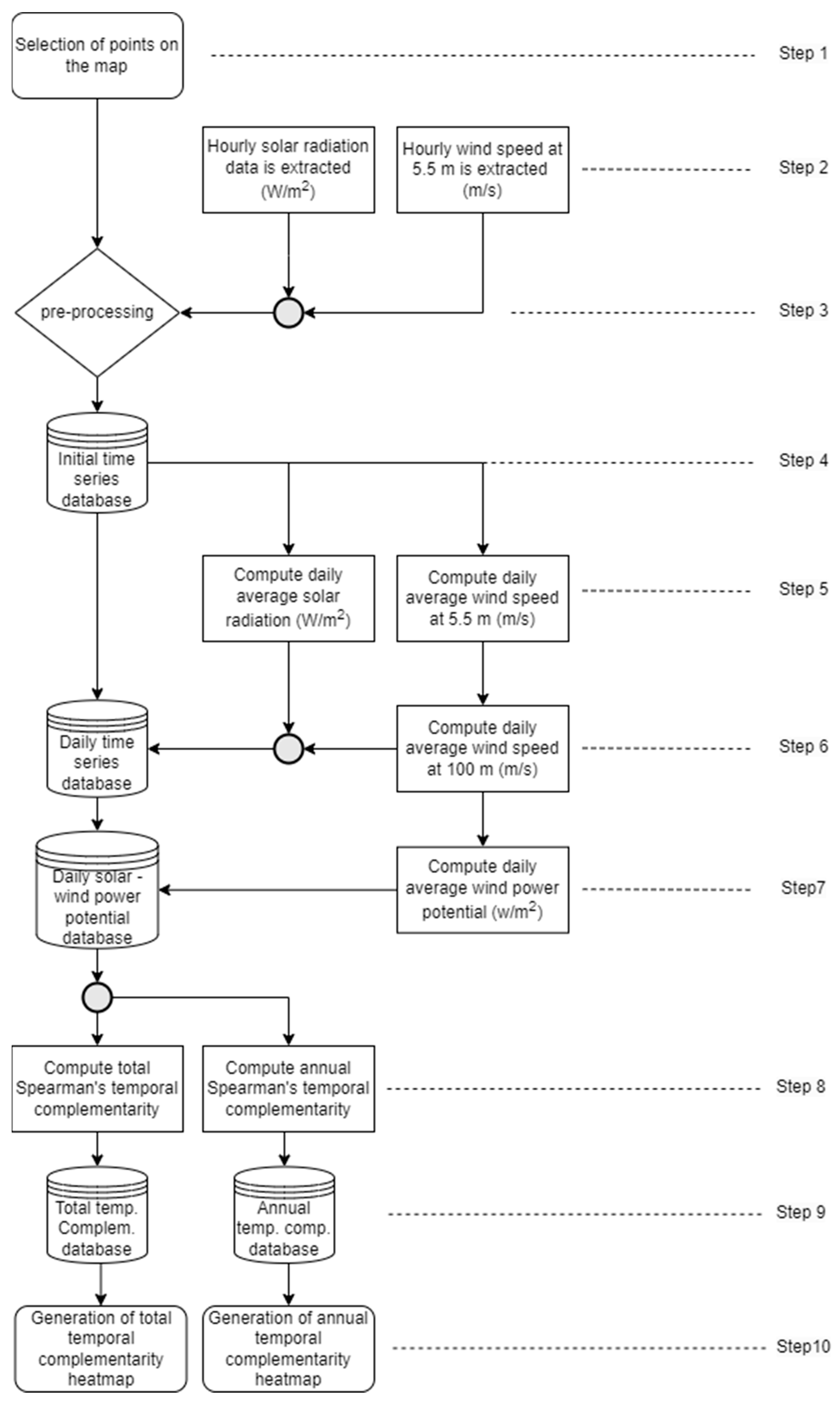
Then, we compute the daily average radiation, in W/m2, and average wind speed at 100 m. Then, the average wind potential, in W/m2, is computed. After that, temporal complementarity is calculated using Spearman’s correlation coefficient, computed for the respective solar and wind power potential time series. We use Spearman’s correlation coefficient because it is a non-parametric estimator of the intensity of the relationship, perhaps non-linear, of two variables [39]. Our methodology, also shown in Figure 4, is the following.
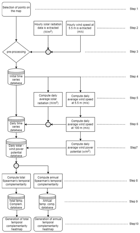
Figure 4.
Flowchart of our methodology to evaluate temporal wind/solar complementarity.
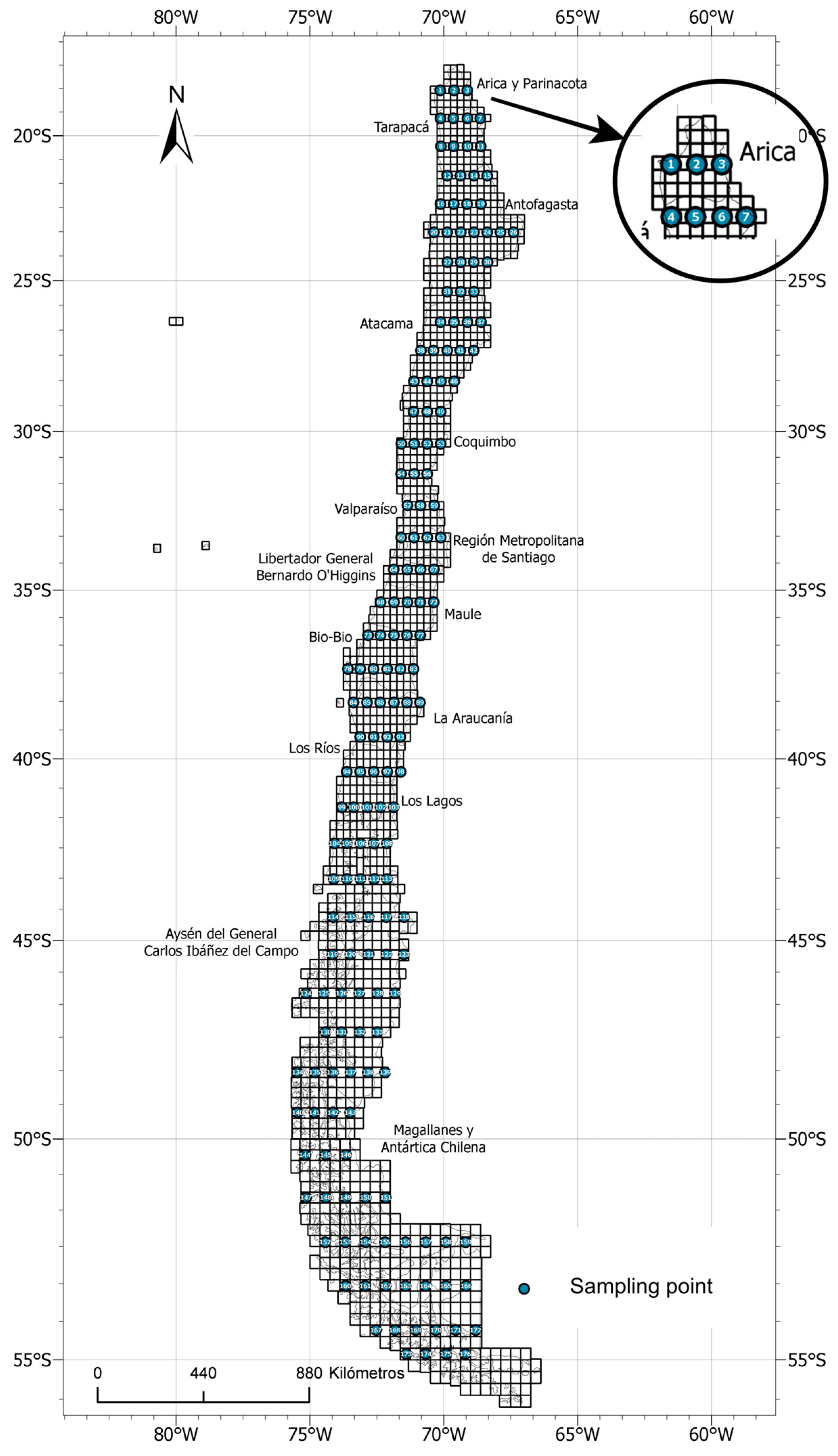
Step 1: Beginning with the geographic map provided by the Chilean Military Geographic Institute (Instituto Geográfico Militar de Chile) [40], which uses a 25 km × 25 km grid. The measurement point selection is like in [41], where wind speed measurement points are separated by 1/4 degrees of latitude and 1/3 degrees of longitude.
We select points 50 km away in longitude and 100 km in latitude, obtaining 176 points covering the whole continental territory of Chile. Each point is composed of an ID and its longitude and latitude.
Step 2: For each point obtained, we extract from “Explorador Solar” the hourly time series for solar radiation and wind speed at 5.5 m from 2004 to 2016. “Explorador Solar” is a public database of superficial solar irradiance for Chile based on data obtained from a radiative transference irradiance model for clear skies and an empiric model from geostationary satellites for cloudy days. The mean percentage error of the model in the hourly time series of global horizontal irradiance is 0.73% [38].
Step 3: We then pre-process the around 40 million resulting values. If a point does not have information, it is computed by interpolating two neighbor points.
Step 4: A usable database of hourly solar radiation and wind speed at 5.5 m from 2004 to 2016 is obtained on 176 geographical points selected in Step 1.
Step 5: Using the Python programming language, the daily averages of solar radiation and wind speed at 5.5 m are computed. The pseudocode of this step and the following is shown in Algorithm 1.
Step 6: We compute the daily average of wind speed at 100 m using Hellman’s exponential law for each day considered.
where:
i: 5.5 m.
h: 100 mm.
Vi: wind speed at 5.5 m.
Vh: wind speed at 100 m.
α: Hellman’s exponent, depending on the terrain rugosity.
Table 2 shows the different values considered for each point in the case study.
| Algorithm 1. Pseudocode to compute the daily averages of solar radiation and wind power. |
| Receives: Points (set of points to study) vel (hourly 5 m wind speed time series) ghi (hourly solar power time series) Days ← ObtainDaysFromTimeSeries(vel, ghi) Years ← ObtainYearsFromDays(Days) for day in Days: for point in Points: Pot100m_eol[day, point] ← EstimatewindPower(vel[day, cell]) meanPot100m_eol[day, point] ← ComputeDailywindPower(Eol_100m, day, ce point ll) meanGhi[day, point] ← ComputeDailySolarPower(ghi, day, point) for point in Points: for year in Years: windPowerTimeSeriesYear ← windPowerTimeSeriesOfYear(meanPot100m_eol, point, year) SolarPowerTimeSeriesYear ← ExtractSolarPowerTimeSeriesOfYear(meanGhi, point, year) Spearman[point, year] ← computeSpearman(windPowerTimeSeriesYear, SolarPowerTimeSeriesYear) Returns: Spearman (the Spearman’s rank correlation coefficient for each point and year) |
Table 2.
Values of Hellman’s exponent for different points of the study area, following [42].
Step 7: Based on the daily average of wind speed at 100 m, we compute the daily average of wind potential in W/m2, making comparable the wind and solar sources, based on the following expression:
where:
Pe/A: daily average wind power potential (W/m2).
ρ: air density (1.12 kg/m2).
V: daily average wind speed at 100 m (m/s).
Step 8: We use Spearman’s correlation coefficient [43] to calculate the temporal complementarity of each point’s daily time series of wind and solar power potential from 2004 to 2016. To categorize correlation, we use the interpretation given in Table 3. We also compute this for the daily time series for each year. For further reference, the following expressions are used to compute Spearman’s coefficient.
where:
Table 3.
Correlation coefficient interpretation. Adapted from [39].
Table 3.
Correlation coefficient interpretation. Adapted from [39].
| Correlation | Interpretation | Kind of Complementarity |
|---|---|---|
| −1 a −0.7 | Strong negative | Strong complementarity |
| −0.7 a −0.3 | Moderate negative | Moderate complementarity |
| −0.3 a 0 | Weak negative | Weak complementarity |
| 0 | No relationship | No relationship |
| 0 a 0.3 | Weak positive | Weak correlation |
| 0.3 a 0.7 | Moderate positive | Moderate correlation |
| 0.7 a 1 | Strong positive | Strong correlation |
: Spearman’s correlation coefficient.
: range of resource j (average daily wind power) on day t.
: range of resource k (average daily solar power) on day t.
T: number of days considered in the analysis (4765 and 365 days, respectively).
S(d2): sum of range differences.
Step 9: We obtain multiple databases: one for the average daily wind–solar temporal complementarity and one for each year from 2004 to 2016.
Step 10: The numerical results are then imported into ArcGIS Pro [44] to generate heat maps from the total and annual complementarity results.
Our methodology has some desirable properties, like the ease of obtaining new results if new or better information on wind speed or solar radiation is available and the possibility of providing graphical representations.
It also has some limitations and potential measurement errors. First, it aggregates information to points in the study area, adding potential errors to the model. Second, it is not dynamic, i.e., it does not prescribe or project its results to the future based on the present and past. Third, it is not guaranteed that different zones will be found each time our methodology is applied to a new dataset.
3. Results
3.1. Total Daily Average Temporal Complementarity
For each point selected, see Figure 5, and based on the daily average data of both wind power and solar radiation from 2004 to 2016, we computed Spearman’s correlation coefficient. The results were entered into a geographical information system, creating a heat map. Red is assigned a correlation value of −1 (strong negative correlation), while blue is set to +1 (strong positive correlation). Figure 6 shows the resulting map, where four zones can be identified.
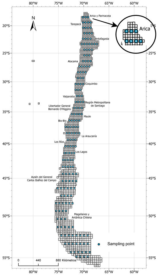
Figure 5.
Points selected from the geographical map of continental Chile are presented as a 25 km × 25 km grid.
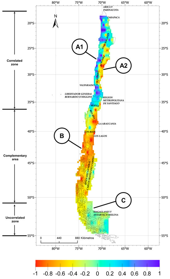
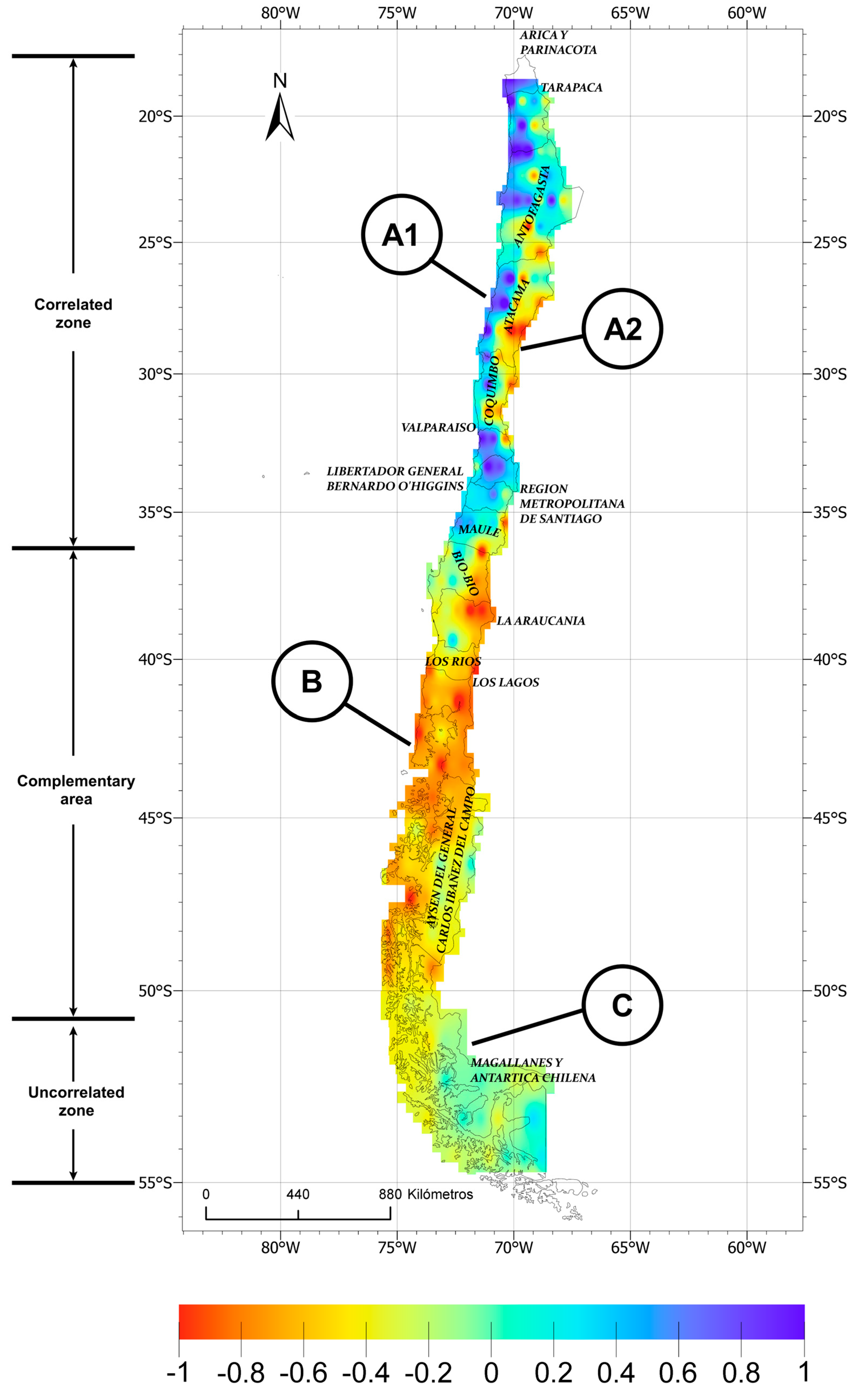
Figure 6.
Total daily average temporal complementarity heat map created with ArcGIS Pro 3.2 software for Spearman’s correlation coefficient, ranging from −1 (red) to 1 (blue).
- Correlated zones: ranging from latitude 18° S to latitude 36° S, covering 72 points (Zone A). Given the different correlation values for the coast and valleys compared to the mountains, we divided Zone A into two subzones: Zones A1 and A2.
- a.1
- Zone A1: At the coast and valleys, covering 45 points from latitude 18° S to latitude 36° S, there is a moderately positive correlated zone, with a median Spearman’s correlation coefficient of +0.44 and an interquartile range of +0.23 to +0.6.
- a.2
- Zone A2: In the mountain area, 27 analysis points were considered, from latitude 25° S to 33° S. There is weak negative complementarity, with a median of −0.18 and an interquartile range between −0.37 and −0.01.
- Complementary zone: covering 77 points, from latitude 36° S to latitude 51° S, there is weak negative complementarity with a median of −0.18 and interquartile range from −0.33 to −0.07 (Zone B).
- Uncorrelated zone: covering 27 points, from latitude 51° S to latitude 55° S, there is weak positive to no correlation, with a median of +0.05 and an interquartile range from −0.04 to +0.12 (Zone C).
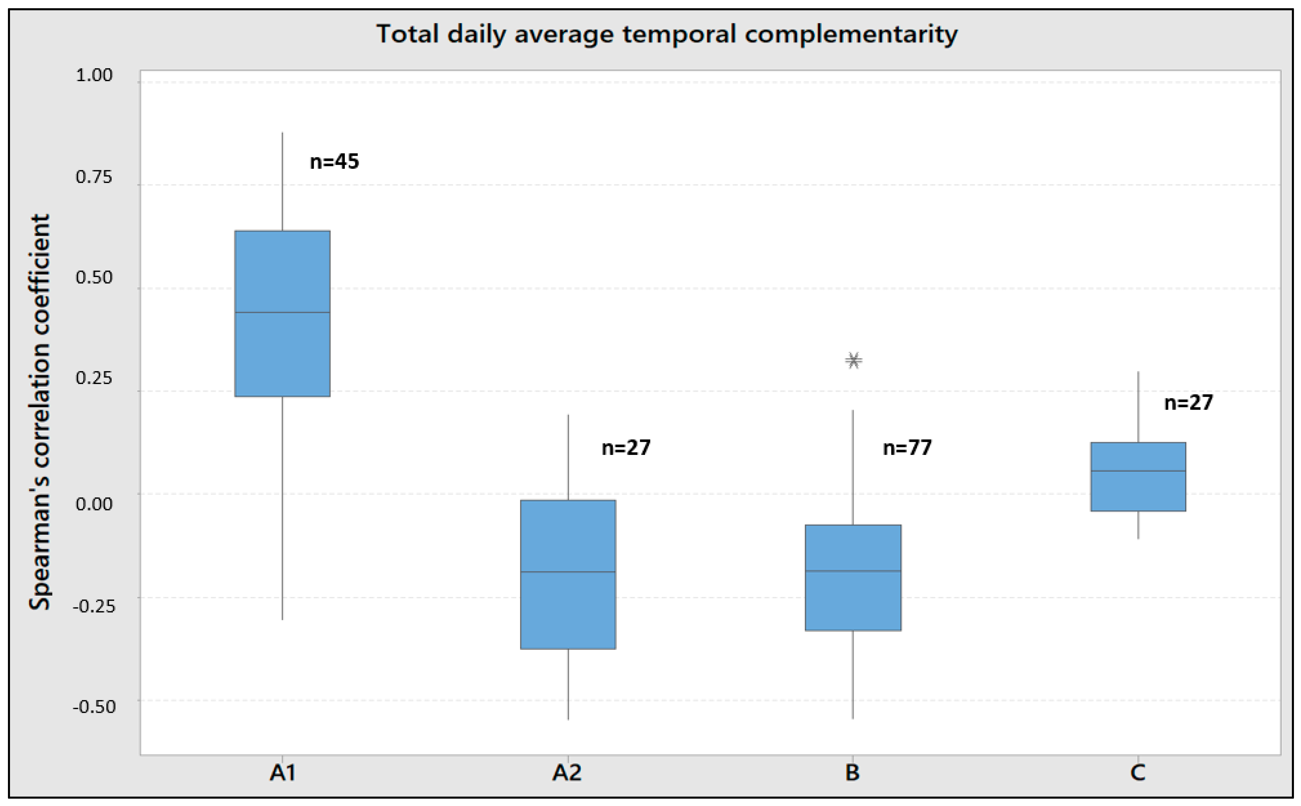
Figure 7 briefly analyzes the resulting zones, showing the number of points and the range of values for Spearman’s correlation coefficient. It shows that the zones have very different characteristics, see, for example, Zones A1, B, and C, and if two zones are similar in dispersion, they are geographically different, see Zones A2 and B.
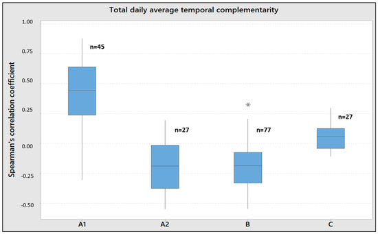
Figure 7.
Dispersion diagram of Spearman’s correlation coefficient for the points in the different zones found, created with Minitab 18 software, where * denotes outliers.
3.2. Daily Average Temporal Complementarity per Year
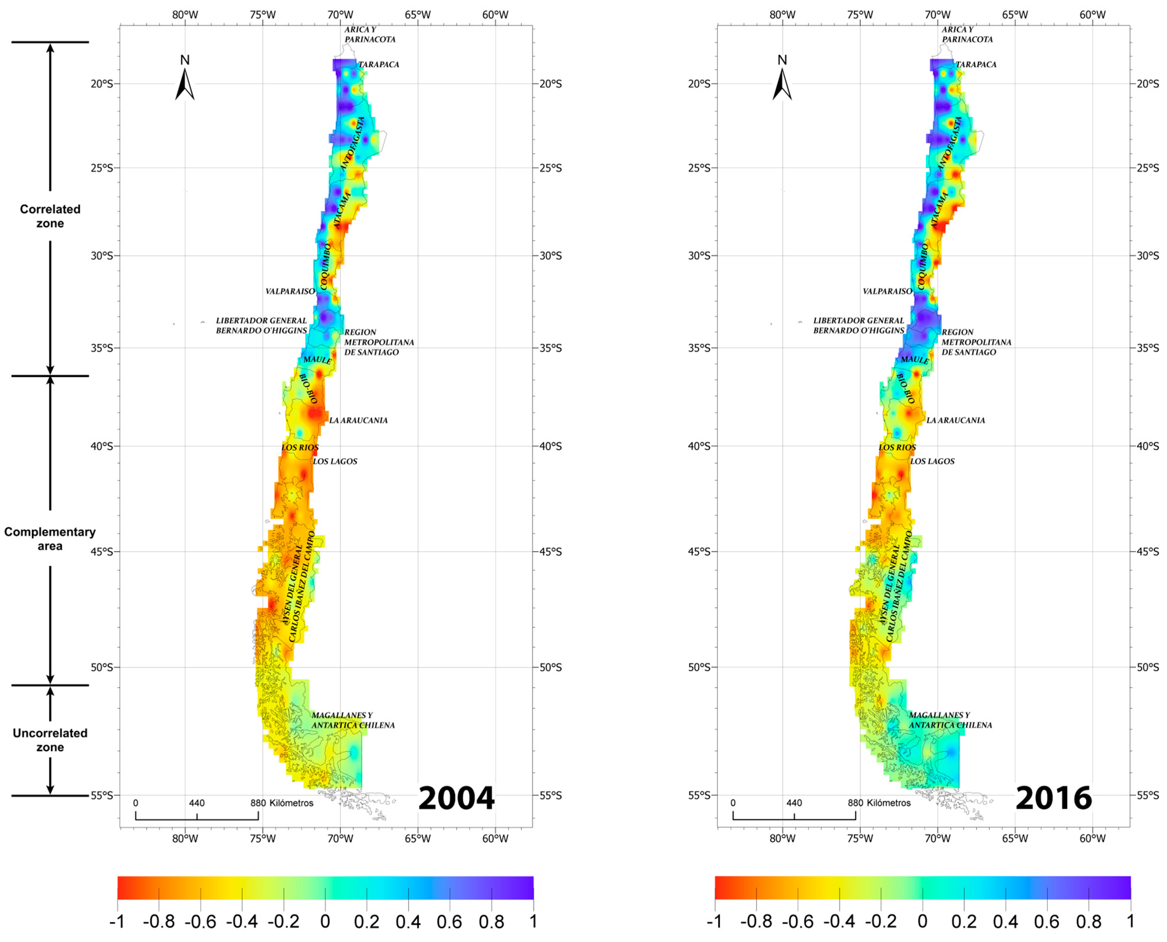
We now repeat the analysis for each year covered by the data. The results show that the zones identified before remaining valid, with variations in the intensity of the complementarity, i.e., the level of correlation. Figure 8 shows a comparison between years 2004 and 2016.
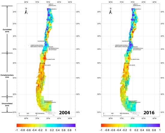
Figure 8.
Daily average temporal complementarity per year. Comparison of 2004 versus 2016 for Spearman’s correlation coefficient, ranging from −1 (red) to 1 (blue).
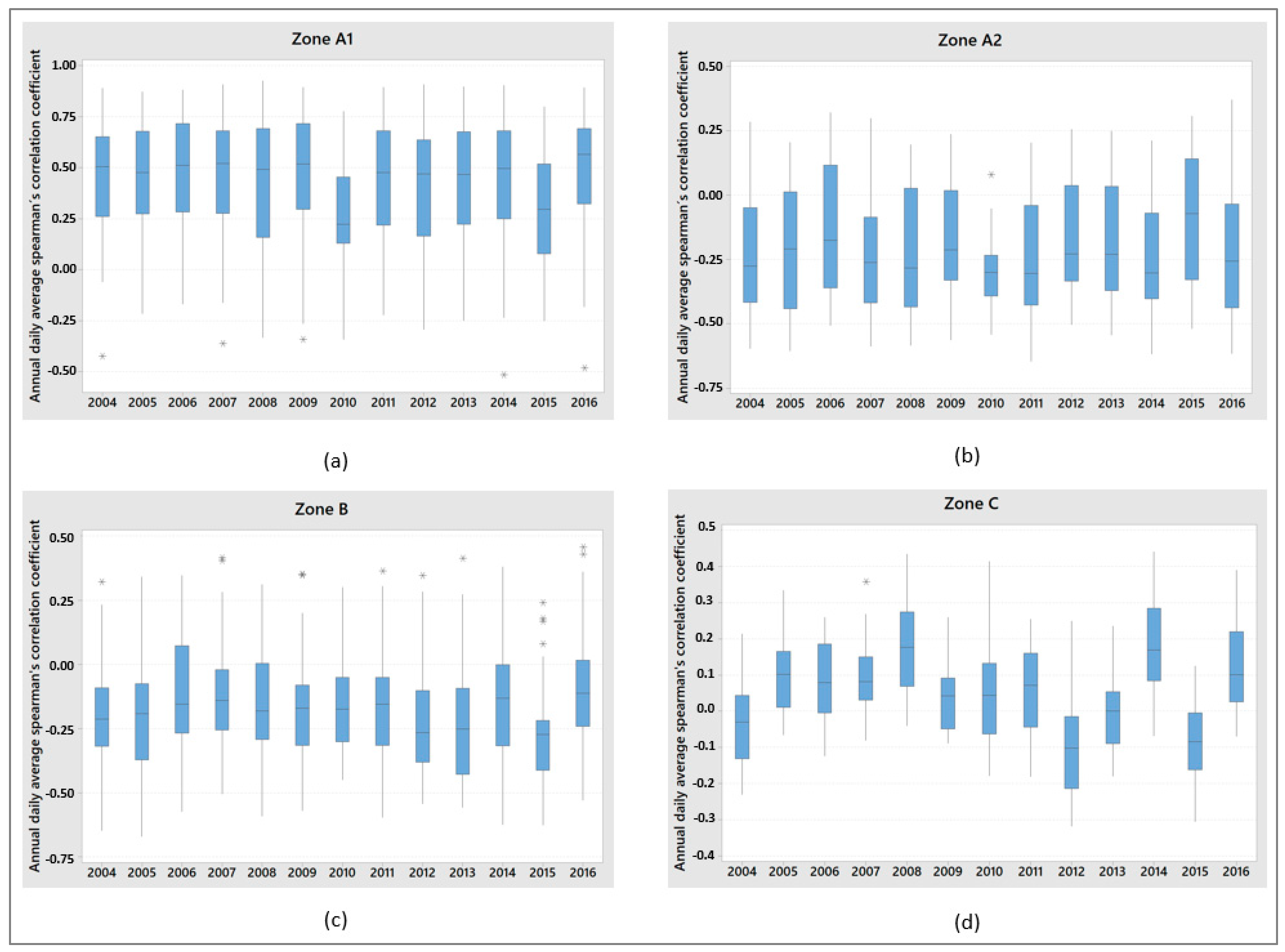
Figure 9a shows the daily average temporal complementarity values for Zone A1 for each year considered. Note that the median is relatively stable, with the value of Spearman’s coefficient around +0.5, i.e., moderate positive correlation, except for years 2010 and 2015, where it is reduced to around +0.25. There is also negative kurtosis, while interquartile ranges and extreme points remain uniform for the period studied.
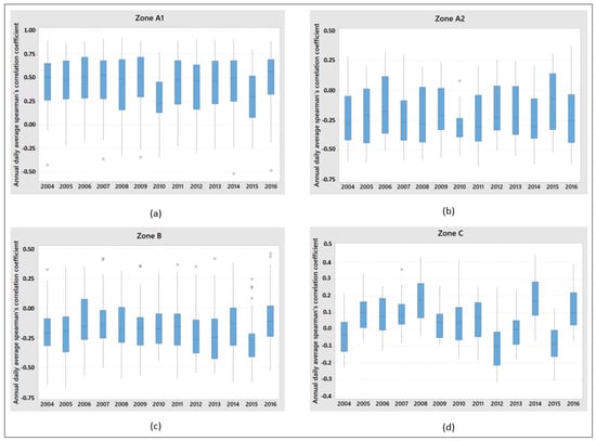
Figure 9.
Evolution of daily average temporal complementarity from 2004 to 2016 for the previously identified zones. (a) Zone A1; (b) Zone A2; (c) Zone B; (d) Zone C, and where * denotes outliers.
Figure 9b is analogous to Figure 9a, but this time for Zone A2, where the median remains stable around −0.25, i.e., weak negative correlation, except for 2015, where it goes up to 0, i.e., no correlation. Positive kurtosis and stable extreme values but dispersion in the interquartile ranges exist.
Figure 9c shows the results obtained for Zone B, where the median varies in time without a clear tendency. Again, the extreme values remain uniform, with weak dispersion of the interquartile ranges. Note also that there are more atypical data points than the previous zones.
Figure 9d corresponds to Zone C, where the median oscillates between −0.08 and +0.17, i.e., without correlation. There are also no clear tendencies in the interquartile ranges and extreme values.
We now analyze graphically the complementarity for points of interest. We select a point inside each zone and then graph the daily averages for both wind and solar power potential for 2014.
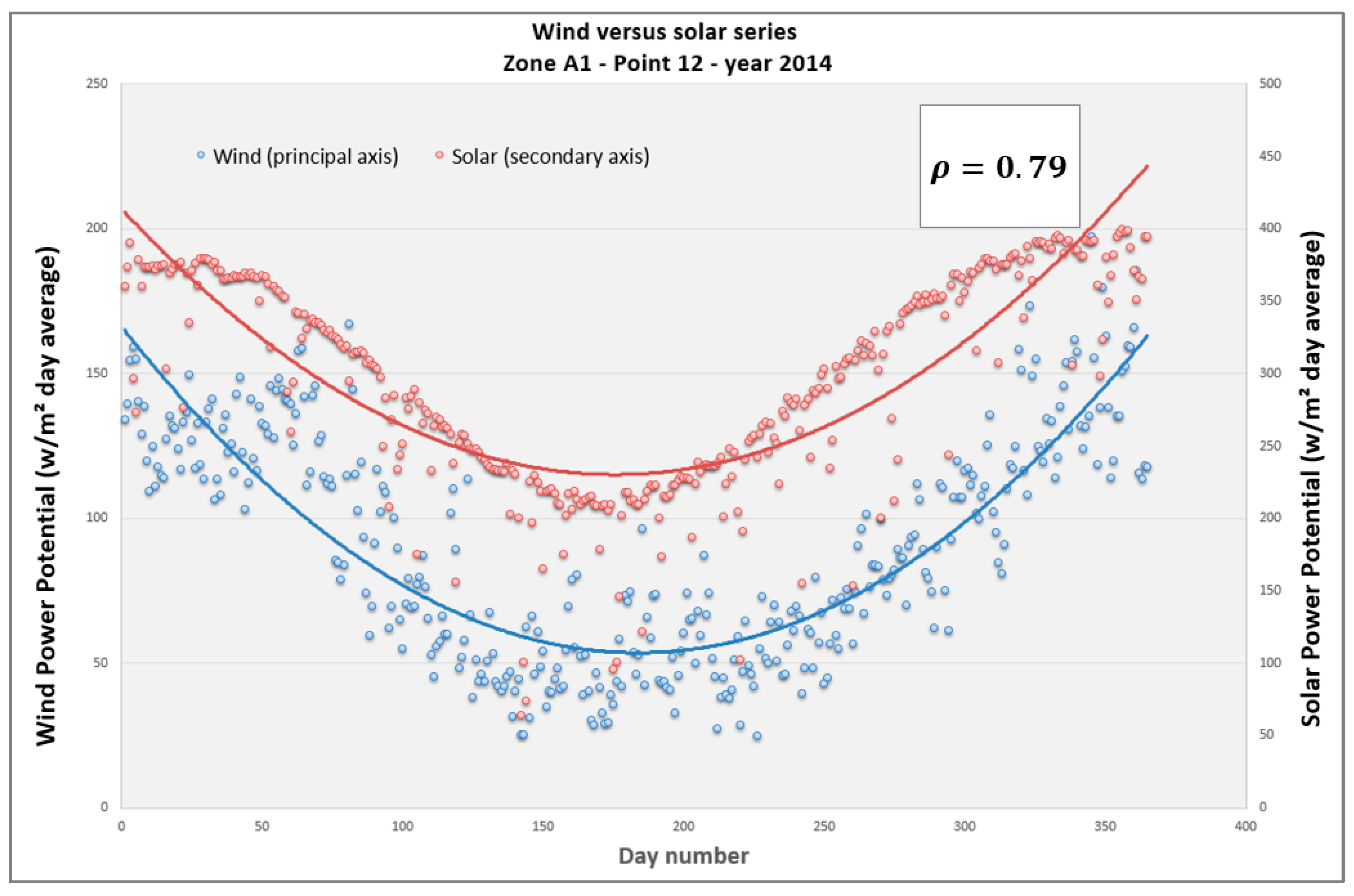
Figure 10 shows the results for Zone A1, where point 12 is selected. At this point, the value of Spearman’s coefficient is +0.79, i.e., a strong positive correlation. In the figure, we plot a trend curve for both time series, where both achieve their maximums in summer and minimums in winter, as expected.
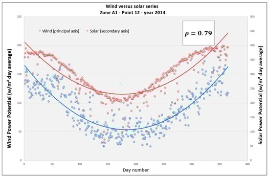
Figure 10.
Wind and solar daily average power potential time series for Zone A1, point 12, year 2014.
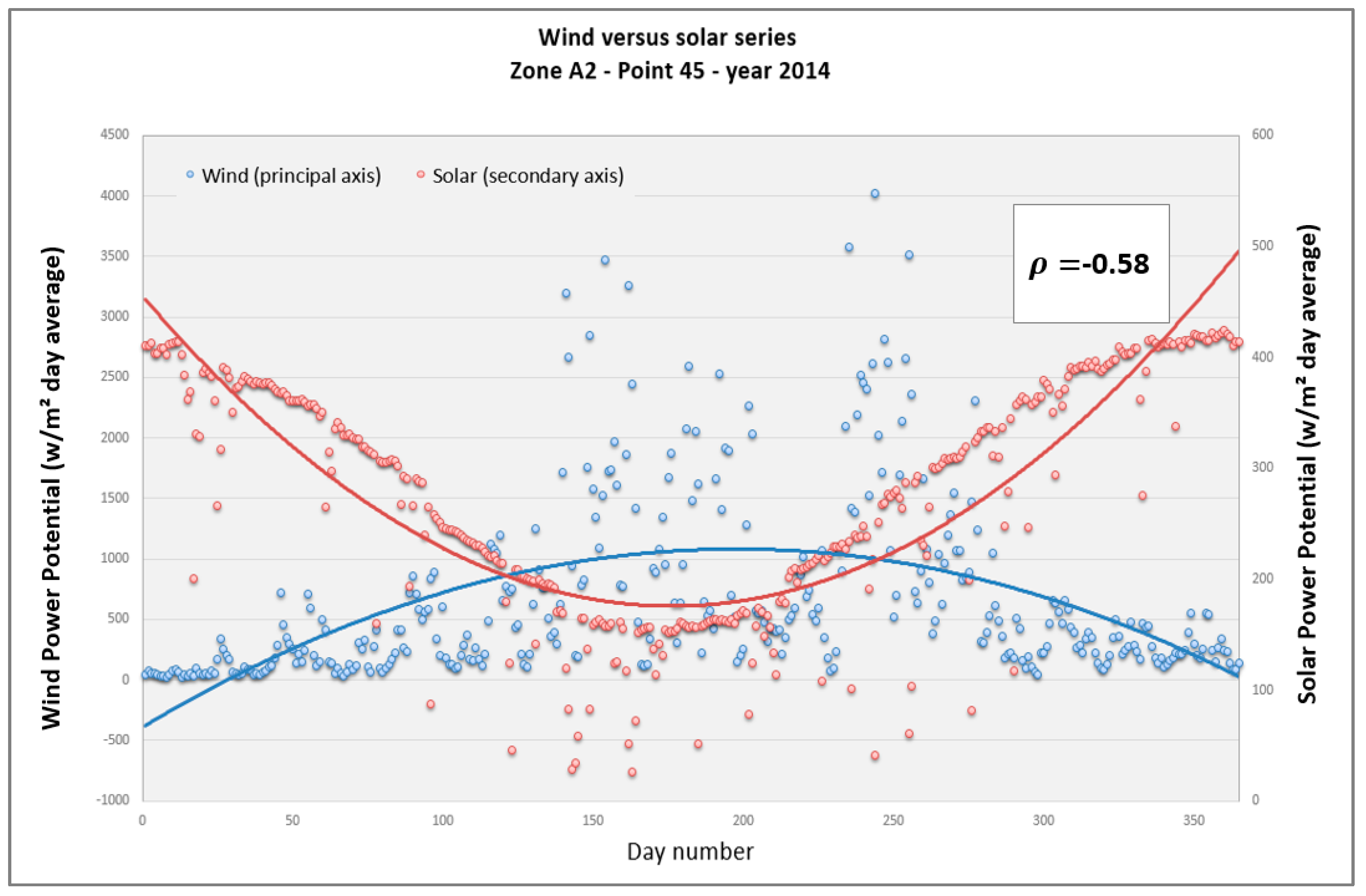
Figure 11 shows the results obtained for point 45 in Zone A2, where the Spearman’s correlation coefficient value is −0.58, i.e., moderate negative correlation. The solar time series achieves its maximum in summer and minimum in winter. The wind time series reaches its maximum in winter with a very high dispersion.
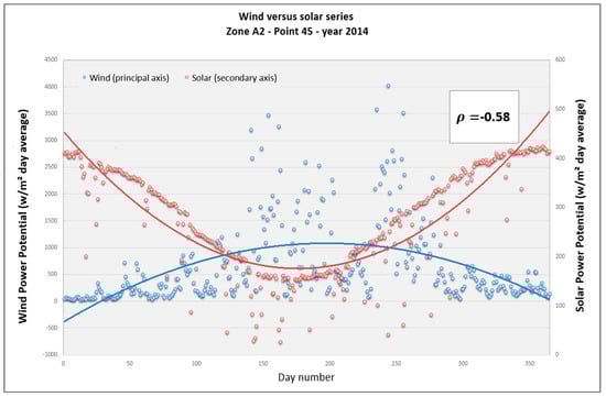
Figure 11.
Wind and solar daily average power potential time series for Zone A2, point 45, year 2014.
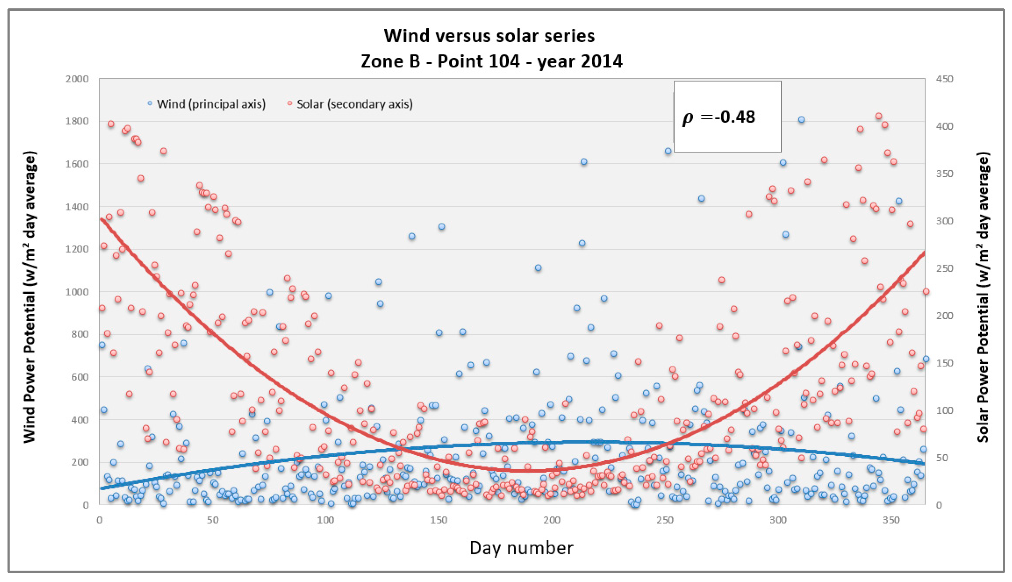
Figure 12 presents the results for point 104 in Zone B, where Spearman’s correlation coefficient is −0.48, i.e., moderate negative correlation. We note that the solar radiation time series achieves its maximum in summer and minimum in winter, but the results have a significant dispersion. The wind time series reaches its maximum in winter, with large dispersion in the values obtained.
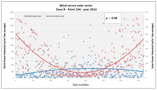
Figure 12.
Wind and solar daily average power potential time series for Zone B, point 104, year 2014.
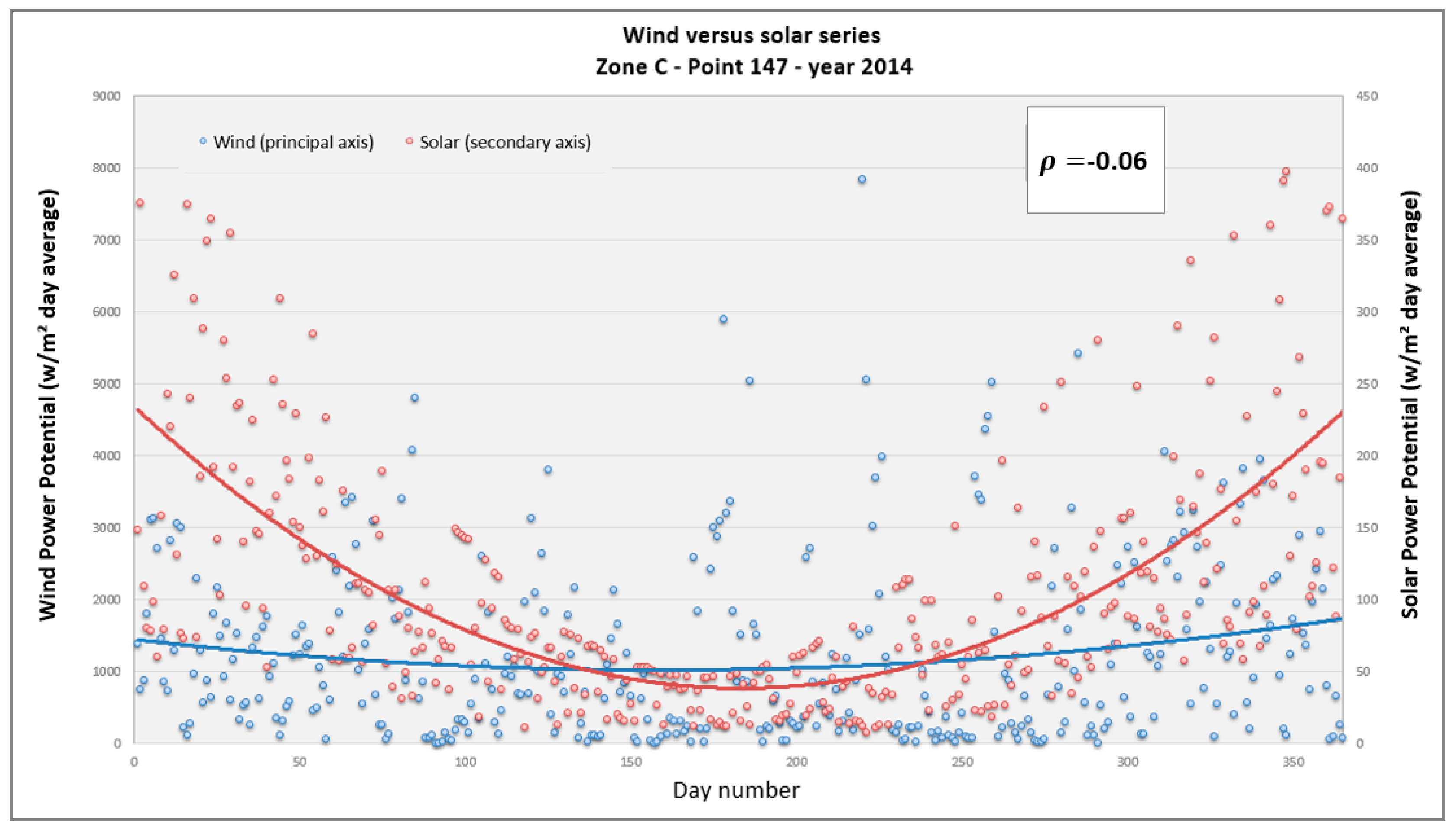
Finally, Figure 13 shows the results obtained for point 147 in Zone B, where the Spearman’s correlation coefficient value is −0.06, i.e., weak to null negative correlation. The behavior of the time series is similar to the previous figure.
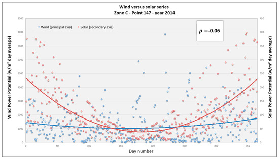
Figure 13.
Wind and solar daily average power potential time series for Zone C, point 147, year 2014.
3.3. Statistical Analysis
In this section, we aim to check if the data used and the zones obtained are valid statistically. We perform a significance test for each point, a statistical characterization, and mean test for each zone and a statistical analysis of the annual evolution of the temporal complementarity for each zone.
3.3.1. Significance Test for Each Point
We define as a sample the values of Spearman’s coefficient obtained for each point in the timespan from 2004 to 2016 (Section 3.1) and the population accordingly.
Let
- -
- Null hypothesis (H0): there is no significant correlation between daily average solar radiation and daily average wind potential.
- -
- Alternative hypothesis (H1): a significant correlation exists between daily average solar radiation and daily average wind potential.
We consider significance level α = 0.05 (5%) and number of data points N = 4745 for each geographical point, obtaining ρc = +0.028 as the critical value of Spearman’s coefficient. If |ρ| > ρc, we must reject H0 and accept H1, i.e., the correlation value is significant. If |ρ| < ρc, then we cannot reject H0, i.e., the value of ρ is not statistically significant.
Figure 14 and Table 4 show that the correlation coefficients are not statistically significant in 9 out of the 176 points. This means that if we select a year at random as a sample, in any of the 167 significant points, there is a probability of at least 95% that they may have a significant correlation. At the same time, it is impossible to make such a claim for the nine remaining. The nine non-significant points are shown in Table 4.
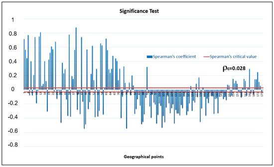
Figure 14.
Spearman’s coefficient significance level for each geographic point, corresponding to total daily average temporal complementarity.
Table 4.
List of statistically non-significative geographical points.
3.3.2. Significance Test per Zone
We want to know if each zone’s correlation is statistically significant. We perform a mean test for each zone, see Table 5. We also report the results on the p-values in Table 6. We define the mean of a zone as the average of the wind–solar complementarity computed using Spearman’s correlation coefficient to all the points in the zone for the time considered. The mean test and p-value are computed following [45,46].
Table 5.
Mean test for the correlations obtained in each zone.
Table 6.
Results of the mean test for each zone.
In this case, we state
- -
- Null hypothesis H0: μ = 0.
- -
- Alternative hypothesis H1: μ ≠ 0.
The results show that, as p < 0.05 and the confidence intervals do not contain 0, we can reject the respective null hypotheses and accept the alternative hypotheses. Specifically, the correlation is significant in Zones A1, A2, and B, while it is marginally significant in Zone C.
4. Conclusions
This work studied the temporal complementarity between wind potential and solar radiation in the continental Chilean territory. We used Spearman’s correlation coefficient to compute the complementarity, given that it is a non-parametric indicator that defines the strength and direction of the variable ranges. This coefficient can be used even if the relation is non-linear, the variables are non-normally distributed, and the variances are different.
For our analysis, we computed the daily average wind and solar power potential time series from 2004 to 2016 from hourly data from 176 geographical points extracted from a public database named “Explorador Solar” [38].
Our analysis showed four differentiated geographical zones in the continental Chilean territory regarding complementarity.
- Zone A1 corresponds to the coast and central valleys in the country’s north, from latitude 18° S to latitude 36° S, with moderate positive correlation, median +0.44, and interquartile range from −0.3 to +0.87.
- Zone A2 corresponds to the mountains in the country’s north, ranging from 25° S to latitude 33° S, with weak negative complementarity, median −0.18, and interquartile range from −0.54 to +0.19.
- Zone B, corresponding to the center and south part of the country, from latitude 36° S to latitude 51° S, has moderate negative complementarity, with a median of −0.18 and interquartile range from −0.54 to +0.32.
- Finally, Zone C, located in the very south of the country, from latitude 51° S to latitude 55° S, has a weak positive to null correlation, a median of +0.05, and an interquartile range from −0.1 to +0.29.
After analyzing the complementarity in each year, we characterized each zone.
- Zone A1 has a stable median, interquartile range, and extreme values for the years considered, i.e., from 2004 to 2016, and negative kurtosis.
- Zone A2 has uniform median and extreme values, but there is dispersion in the interquartile ranges. We also noted that, in most years, it shows positive kurtosis.
- Zone B has a non-uniform median, stable extreme values, and non-stable interquartile ranges.
- Finally, Zone C has a non-uniform median, extreme values, and interquartile range.
We tested the statistical validity of our results through a significance test for Spearman’s coefficient obtained in all the geographical points considered. The results obtained for 167 of the 176 are statistically significant. The significance test for each zone showed that Zones A1, A2, and B have a statistically significant correlation, while Zone C is marginally significant.
Given that Chile aims to have a 100% renewable electric energy generation matrix by installing wind and photovoltaic generation and new storage systems, this work provides a way to this energy transition. We suggest incentivizing the development of distributed hybrid generation, taking advantage of the temporal complementarity stated in the zones identified in this work. We think that considering our obtained complementarity heat maps is the first step to reducing the investment costs of energy generation and storage. A potential place for these incentives could be Zone A2, where large mining companies are located, demanding massive amounts of electric energy. Implementing wind–solar hybrid generation systems could reduce the energy storage required to meet the demand, reducing investment and operation costs and reducing their carbon footprint.
As future research lines, we want to tackle:
- Spatial complementarity,
- The sizing of distributed hybrid generation systems considering the existing complementarity levels,
- The effect of climate change in the wind–solar complementarity.
Author Contributions
J.L.M.-P. worked on every task; A.L.-V. focused on programming, translation, and general manuscript review, while L.S. and F.S. supervised the whole work and performed a general review. All the authors analyzed the results obtained. All authors have read and agreed to the published version of the manuscript.
Funding
This research received no external funding.
Data Availability Statement
All the data can be provided by request to the corresponding author.
Conflicts of Interest
The authors do not have conflicts of interest.
References
- IPCC. Climate Change 2023: Synthesis Report. Contribution of Working Groups I, II and III to the Sixth Assessment Report of the Intergovernmental Panel on Climate Change. 2023. Available online: https://www.ipcc.ch/report/ar6/syr/downloads/report/IPCC_AR6_SYR_FullVolume.pdf (accessed on 9 April 2024).
- ONU. Acuerdo de París de la Convención Marco de las Naciones Unidas Sobre el Cambio Climático (UNFCCC). 2015. Available online: https://www.refworld.org.es/docid/602021b64.html (accessed on 9 April 2024).
- IEA. Net Zero Roadmap: A Global Path to Keep the 1.5 °C Target within Reach, IEA, Paris. 2023. Available online: https://www.iea.org/reports/net-zero-roadmap-a-global-pathway-to-keep-the-15-0c-goal-in-reach (accessed on 9 April 2024).
- Coordinador Eléctrico Nacional. Hoja de Ruta Para una Transición Energética Acelerada, Visión del Coordinador Eléctrico Nacional. 2022. Available online: https://www.coordinador.cl/wp-content/uploads/2022/06/8_digital_Informe_Coordinador_2.5.pdf (accessed on 9 April 2024).
- Generadoras. Boletin Generadoras de Chile-Septiembre 2023. 2023. Available online: https://generadoras.cl/documentos/boletines/boletin-generadoras-de-chile-septiembre-2023 (accessed on 9 April 2024).
- Pérez Odeh, R.; Watts, D. Impacts of wind and solar spatial diversification on its market value: A case study of the Chilean electricity market. Renew. Sustain. Energy Rev. 2019, 111, 442–461. [Google Scholar] [CrossRef]
- Ministerio de Energía; Gobierno de Chile. Plan Nacional de Eficiencia Energética 2022–2026. 2022. Available online: https://energia.gob.cl/sites/default/files/eficiencia-energetica_16-nov.pdf (accessed on 9 April 2024).
- International Energy Agency. The Evolution of Energy Efficiency Policy to Support Clean Energy Transitions; OECD: Paris, France, 2023. [Google Scholar] [CrossRef]
- Khan, K.A.; Quamar, M.M.; Al-Qahtani, F.H.; Asif, M.; Alqahtani, M.; Khalid, M. Smart grid infrastructure and renewable energy deployment: A conceptual review of Saudi Arabia. Energy Strategy Rev. 2023, 50, 101247. [Google Scholar] [CrossRef]
- Rey-Costa, E.; Elliston, B.; Green, D.; Abramowitz, G. Firming 100% renewable power: Costs and opportunities in Australia’s National Electricity Market. Renew. Energy 2023, 219, 119416. [Google Scholar] [CrossRef]
- Song, X.; Zhang, H.; Fan, L.; Zhang, Z.; Peña-Mora, F. Planning shared energy storage systems for the spatio-temporal coordination of multi-site renewable energy sources on the power generation side. Energy 2023, 282, 128976. [Google Scholar] [CrossRef]
- Auguadra, M.; Ribó-Pérez, D.; Gómez-Navarro, T. Planning the deployment of energy storage systems to integrate high shares of renewables: The Spain case study. Energy 2023, 264, 126275. [Google Scholar] [CrossRef]
- Akrouch, M.A.; Chahine, K.; Faraj, J.; Hachem, F.; Castelain, C.; Khaled, M. Advancements in cooling techniques for enhanced efficiency of solar photovoltaic panels: A detailed comprehensive review and innovative classification. Energy Built Environ. 2023, in press. [CrossRef]
- Al Sumarmad, K.A.; Sulaiman, N.; Wahab, N.I.A.; Hizam, H. Energy Management and Voltage Control in Microgrids Using Artificial Neural Networks, PID, and Fuzzy Logic Controllers. Energies 2022, 15, 303. [Google Scholar] [CrossRef]
- Kharrich, M.; Selim, A.; Kamel, S.; Kim, J. An effective design of hybrid renewable energy system using an improved Archimedes Optimization Algorithm: Acase study of Farafra, Egypt. Energy Convers. Manag. 2023, 283, 116907. [Google Scholar] [CrossRef]
- Naderipour, A.; Kamyab, H.; Klemeš, J.J.; Ebrahimi, R.; Chelliapan, S.; Nowdeh, S.A.; Abdullah, A.; Hedayati Marzbali, M. Optimal design of hybrid grid-connected photovoltaic/wind/battery sustainable energy system improving reliability, cost and emission. Energy 2022, 257, 124679. [Google Scholar] [CrossRef]
- Agajie, T.F.; Ali, A.; Fopah-Lele, A.; Amoussou, I.; Khan, B.; Velasco, C.L.R.; Tanyi, E. A Comprehensive Review on Techno-Economic Analysis and Optimal Sizing of Hybrid Renewable Energy Sources with Energy Storage Systems. Energies 2023, 16, 642. [Google Scholar] [CrossRef]
- Jurasz, J.; Canales, F.A.; Kies, A.; Guezgouz, M.; Beluco, A. A review on the complementarity of renewable energy sources: Concept, metrics, application and future research directions. Sol. Energy 2020, 195, 703–724. [Google Scholar] [CrossRef]
- Pedruzzi, R.; Silva, A.R.; Soares dos Santos, T.; Araujo, A.C.; Cotta Weyll, A.L.; Lago Kitagawa, Y.K.; Nunes da Silva Ramos, D.; Milani de Souza, F.; Almeida Narciso, M.V.; Saraiva Araujo, M.L.; et al. Review of mapping analysis and complementarity between solar and wind energy sources. Energy 2023, 283, 129045. [Google Scholar] [CrossRef]
- Gallardo, R.P.; Ríos, A.M.; Ramírez, J.S. Analysis of the solar and wind energetic complementarity in Mexico. J. Clean. Prod. 2020, 268, 122323. [Google Scholar] [CrossRef]
- Magaña-González, R.C.; Rodríguez-Hernández, O.; Canul-Reyes, D.A. Analysis of seasonal variability and complementarity of wind and solar resources in Mexico. Sustain. Energy Technol. Assess. 2023, 60, 103456. [Google Scholar] [CrossRef]
- Costoya, X.; de Castro, M.; Carvalho, D.; Gómez-Gesteira, M. Assessing the complementarity of future hybrid wind and solar photovoltaic energy resources for North America. Renew. Sustain. Energy Rev. 2023, 173, 113101. [Google Scholar] [CrossRef]
- Guo, Y.; Ming, B.; Huang, Q.; Yang, Z.; Kong, Y.; Wang, X. Variation-based complementarity assessment between wind and solar resources in China. Energy Convers. Manag. 2023, 278, 116726. [Google Scholar] [CrossRef]
- Ren, G.; Wan, J.; Liu, J.; Yu, D. Spatial and temporal assessments of complementarity for renewable energy resources in China. Energy 2019, 177, 262–275. [Google Scholar] [CrossRef]
- Gelaro, R.; McCarty, W.; Suárez, M.J.; Todling, R.; Molod, A.; Takacs, L.; Randles, C.A.; Darmenov, A.; Bosilovich, M.G.; Reichle, R.; et al. The Modern-Era Retrospective Analysis for Research and Applications, Version 2 (MERRA-2). J. Clim. 2017, 30, 5419–5454. [Google Scholar] [CrossRef]
- Couto, A.; Estanqueiro, A. Assessment of wind and solar PV local complementarity for the hybridization of the wind power plants installed in Portugal. J. Clean. Prod. 2021, 319, 128728. [Google Scholar] [CrossRef]
- Nogueira, E.C.; Morais, R.C.; Pereira, A.O. Offshore Wind Power Potential in Brazil: Complementarity and Synergies. Energies 2023, 16, 5912. [Google Scholar] [CrossRef]
- Fernandes, P.C.B.; Risso, A.; Beluco, A. Chapter 5—A survey on temporal and spatial complementarity between wind and solar resources along the coast of northeastern Brazil. In Complementarity of Variable Renewable Energy Sources; Jurasz, J., Beluco, A., Eds.; Academic Press: Cambridge, MA, USA, 2022; pp. 99–120. [Google Scholar] [CrossRef]
- Beluco, A.; de Souza, P.K.; Krenzinger, A. A dimensionless index evaluating the time complementarity between solar and hydraulic energies. Renew. Energy 2008, 33, 2157–2165. [Google Scholar] [CrossRef]
- Cantão, M.P.; Bessa, M.R.; Bettega, R.; Detzel, D.H.M.; Lima, J.M. Evaluation of hydro-wind complementarity in the Brazilian territory by means of correlation maps. Renew. Energy 2017, 101, 1215–1225. [Google Scholar] [CrossRef]
- Cantor, D.; Ochoa, A.; Mesa, O. Total Variation-Based Metrics for Assessing Complementarity in Energy Resources Time Series. Sustainability 2022, 14, 8514. [Google Scholar] [CrossRef]
- Henao, F.; Viteri, J.P.; Rodríguez, Y.; Gómez, J.; Dyner, I. Annual and interannual complementarities of renewable energy sources in Colombia. Renew. Sustain. Energy Rev. 2020, 134, 110318. [Google Scholar] [CrossRef]
- Gonzalez-Salazar, M.; Poganietz, W.R. Evaluating the complementarity of solar, wind and hydropower to mitigate the impact of El Niño Southern Oscillation in Latin America. Renew. Energy 2021, 174, 453–467. [Google Scholar] [CrossRef]
- Viviescas, C.; Lima, L.; Diuana, F.A.; Vasquez, E.; Ludovique, C.; Silva, G.N.; Huback, V.; Magalar, L.; Szklo, A.; Lucena, A.F.P.; et al. Contribution of Variable Renewable Energy to increase energy security in Latin America: Complementarity and climate change impacts on wind and solar resources. Renew. Sustain. Energy Rev. 2019, 113, 109232. [Google Scholar] [CrossRef]
- Garcia, M.; Oliva, S. Technical, economic, and CO2 emissions assessment of green hydrogen production from solar/wind energy: The case of Chile. Energy 2023, 278, 127981. [Google Scholar] [CrossRef]
- Camargo, L.R.; Valdes, J.; Macia, Y.M.; Dorner, W. Assessment of on-site steady electricity generation from renewable energy sources in Chile. Energy Procedia 2019, 158, 1099–1104. [Google Scholar] [CrossRef]
- Vargas-Ferrer, P.; Álvarez-Miranda, E.; Tenreiro, C.; Jalil-Vega, F. Assessing flexibility for integrating renewable energies into carbon neutral multi-regional systems: The case of the Chilean power system. Energy Sustain. Dev. 2022, 70, 442–455. [Google Scholar] [CrossRef]
- Molina, A.; Falvey, M.; Rondanelli, R. A solar radiation database for Chile. Sci. Rep. 2017, 7, 14823. [Google Scholar] [CrossRef]
- Santabárbara, J. Cálculo del intervalo de confianza para los coeficientes de correlación mediante sintaxis en SPSS. REIRE Rev. D’innovació Recer. Educ. 2019, 12, 1–14. [Google Scholar] [CrossRef]
- IGM. Instituto Geográfico Militar de Chile. Grilla IGM Escala 1:25000 KMZ. Available online: https://www.igm.cl/?page=descargas-gratuitas-igm&menu=1 (accessed on 15 January 2024).
- Zhang, N.; Lu, X.; McElroy, M.B.; Nielsen, C.P.; Chen, X.; Deng, Y.; Kang, C. Reducing curtailment of wind electricity in China by employing electric boilers for heat and pumped hydro for energy storage. Appl. Energy 2016, 184, 987–994. [Google Scholar] [CrossRef]
- Wiernga, J. Representative roughness parameters for homogeneous terrain. Bound.-Layer Meteorol 1993, 63, 323–363. [Google Scholar] [CrossRef]
- Canales, F.A.; Acuña, G.J. Chapter 2—Metrics and indices used for the evaluation of energetic complementarity—A review. In Complementarity of Variable Renewable Energy Sources; Jurasz, J., Beluco, A., Eds.; Academic Press: Cambridge, MA, USA, 2022; pp. 35–55. [Google Scholar] [CrossRef]
- ArcGIS Pro. Software de Representación Cartográfica SIG 2D, 3D y 4D. Available online: https://www.esri.cl/es-cl/productos/arcgis-pro/overview (accessed on 16 January 2024).
- Delgado, R. Probabilidad y Estadística Para Ciencias e Ingenierias. Delta. 2007. Available online: https://books.google.cl/books?id=xbiCKj0vV6kC (accessed on 9 April 2024).
- Sleeper, A. Minitab Demystified. In Demystified. Mcgraw-Hill. 2011. Available online: https://books.google.cl/books?id=cy6E5R2Zv3kC (accessed on 9 April 2024).

Disclaimer/Publisher’s Note: The statements, opinions and data contained in all publications are solely those of the individual author(s) and contributor(s) and not of MDPI and/or the editor(s). MDPI and/or the editor(s) disclaim responsibility for any injury to people or property resulting from any ideas, methods, instructions or products referred to in the content. |
© 2024 by the authors. Licensee MDPI, Basel, Switzerland. This article is an open access article distributed under the terms and conditions of the Creative Commons Attribution (CC BY) license (https://creativecommons.org/licenses/by/4.0/).