Article

Analysis of Energy Efficiency Opportunities for a Public Transportation Maintenance Facility—A Case Study

1
Smart and Small Thermal Systems Laboratory, Center for Environmental Energy Engineering, University of Maryland College Park, 8228 Paint Branch Drive, College Park, MD 20742, USA
2
Department of Materials Engineering, University of Pennsylvania, Philadelphia, PA 19104, USA
*
Author to whom correspondence should be addressed.
Energies 2024, 17(8), 1907; https://doi.org/10.3390/en17081907
Submission received: 5 March 2024 / Revised: 11 April 2024 / Accepted: 12 April 2024 / Published: 17 April 2024
(This article belongs to the Section G: Energy and Buildings)

Abstract

:
A comprehensive energy audit of a light rail maintenance facility was performed to assess its energy performance and identify potential scope for improvements. The facility’s energy use intensity (EUI) for 2022 was 404 kWh/m2—more than double the benchmark EUI for maintenance facilities (151 kWh/m2) recommended by EnergyStar. Furthermore, the load factor was 0.22—significantly lower than the recommended minimum of 0.75 for an efficient building. The energy audit encompassed an in-depth evaluation of the facility’s structural and operational characteristics, comprising HVAC systems, lighting, the building envelope, and energy-intensive machinery. An energy model of the facility was developed to emulate the facility’s energy performance in 2022. Following the energy model’s validation, an analysis was conducted to identify opportunities for improving energy efficiency. Post-implementation of energy efficiency measures for the facility, the projected annual reductions are 1086 MWh of electricity, 5034 GJ of natural gas, utility savings of USD 162,402, and net GHG emissions reductions of 584 metric tons of CO2e. A subsequent 30% reduction in EUI to 283.6 kWh/m2 could be achieved with an 86% improvement in load factor, that is, increasing it from 0.22 to 0.41. This study emphasizes the need for energy audits and modeling for maintenance facilities to reduce Scope 1 and 2 emissions.

1. Introduction

In 2022, U.S. energy consumption peaked at 105 EJ, resulting in a substantial 4.7 gigatonnes of CO2 greenhouse gas emissions [1]. In light of the climate change caused by these emissions, the U.S. Department of Energy [2] anticipates the necessity for advanced technologies to facilitate a transition to clean energy by 2050, given projected increases in both population and business activities. The importance of reducing these emissions has also reignited interest in energy efficiency [3] in that, alongside advanced technologies, enhanced energy efficiency will also be required to achieve emissions targets.
The building sector consumes nearly 30% of energy in the U.S. [4]. Buildings are major contributors to energy consumption and greenhouse gas emissions, making their energy efficiency a vital aspect of any sustainability initiative [5]. In response to the energy and climate crises, Maryland State Governor Wes Moore signed an executive order requiring state-owned facilities to reduce their energy consumption by 20% by 2031 [6]. Furthermore, the Building Energy Performance Standards (BEPS) required by the Maryland Climate Solutions Now Act of 2022 mandate that buildings in Maryland that are 35,000 square feet (~3252 m2) or larger achieve a 20% reduction in net direct GHG emissions, as compared with 2025 levels, by 1 January 2030 and subsequently net-zero direct GHG emissions by 1 January 2040 [7].
To this end, energy audits and energy-efficient practices have become imperative [8]. In one study [9], the effect of a city-wide mandatory audit policy—New York City’s Local Law 87—on building energy use for approximately 4000 buildings was examined using energy data from 2011 to 2016. The results showed that mandatory energy audits negatively impacted energy consumption in office and residential buildings in NYC. It reinstated the idea that energy audits provide only limited incentives to facility owners and building managers to invest in enhancing their energy efficiency owing to barriers such as limited capital access, subjective savings projections, and skeptical pricing in energy markets. Energy audits provide a systematic assessment of a building’s energy use and a set of recommendations for enhancing the building’s energy efficiency [10]. By demonstrating a case study and associated savings, [11] emphasized the importance of comprehensive energy audits. A 77,000 ft2 (7154 m2) office building in upstate New York was audited to gauge potential savings through energy audits. It was found that the facility could potentially save 37% annually, or USD 125,000, upon implementation of the energy efficiency measures. Furthermore, without significantly altering the building design, implementing energy efficiency measures (EEMs) can reduce energy use by 20–30% on average [12]. Twelve building types were assessed over four years, primarily focusing on installing smaller, cheaper HVAC equipment. It was found that most HVAC systems were oversized, and appropriate sizing could reduce a building’s carbon footprint by 16% on average. Energy audits on maintenance buildings are particularly beneficial, as these structures play a crucial role in various industries and critical housing operations that demand optimal energy use for sustainability, cost reduction, and environmental responsibility [9]. These structures house essential equipment, materials, and personnel vital to the efficient functioning and upkeep of operations. Maintenance facilities employ and store heavy-duty equipment, including hoists, cranes, presses, lathes, TIG welding, washers, and milling equipment [13]. To this effect, energy modeling has been a popular tool to emulate a facility’s energy performance and calculate savings by implementing energy efficiency measures [14,15,16]. The physics-informed model (PIM) approach is the preferred choice for analyzing the energy demand of individual buildings based on installed equipment and technologies in the facility [17]. The PIM approach allows assessment of the impact of energy efficiency upgrades on overall building energy consumption. In [18], an energy model for a commercial building was developed to study the electricity savings from a water-to-water heat pump in a commercial building. It was observed that the savings ranged from 20 to 27% on a monthly basis. Regular energy audits can identify energy waste, recommend tailored efficiency measures, and promote sustainable energy usage practices, thereby reducing operational costs and promoting a sustainable future. However, because maintenance facilities vary in operation, the literature on them is limited. This study addresses this gap in knowledge by delving into the importance of energy audits and energy efficiency in maintenance buildings, emphasizing the necessity of this practice for economic and environmental benefits.
While analyzing high-speed railways, [19] assessed the pantograph-catenary system as the most vulnerable part of the traction power system. In [20], different approaches were studied to improve pantograph–catenary performance at a speed of 400 km/h and above. Seven different perspectives were reviewed for future studies to improve the performance of pantograph–catenary systems. In [21], an experimental test of the pantograph–catenary system was conducted at different speeds. They developed a neural network optimization algorithm to find optimal contact performance at different velocities. The optimization algorithm improved the contact quality of the pantograph–catenary system at 380 km/h. With different countries pushing towards carbon reduction, high-speed trains have become a focus of electricity consumption reduction. To this effect, maglev trains would rely on renewable electricity. In [22], a novel superconducting magnetic energy storage (SMES) system in conjunction with distributed renewable energy sources was explored. Using distributed renewable energy sources, clean electricity can be provided to power these trains without heavily relying on the grid, while the SMES system actively responds to the power demand of maglev trains during acceleration and braking conditions by rapidly releasing and absorbing energy. The Maryland Transit Administration (MTA) handles the operation and maintenance of multiple mass transportation methods for the State of Maryland. As part of a larger project, we prioritized the MTA’s maintenance facilities for auditing using the ranking software developed in [23], which ranks facilities based on different energy metrics, such as EUI, total GHG emissions, and energy-saving potential. We modeled the energy consumption of buildings that were heavy energy consumers to identify the deficiencies contributing to subpar energy performance [24].
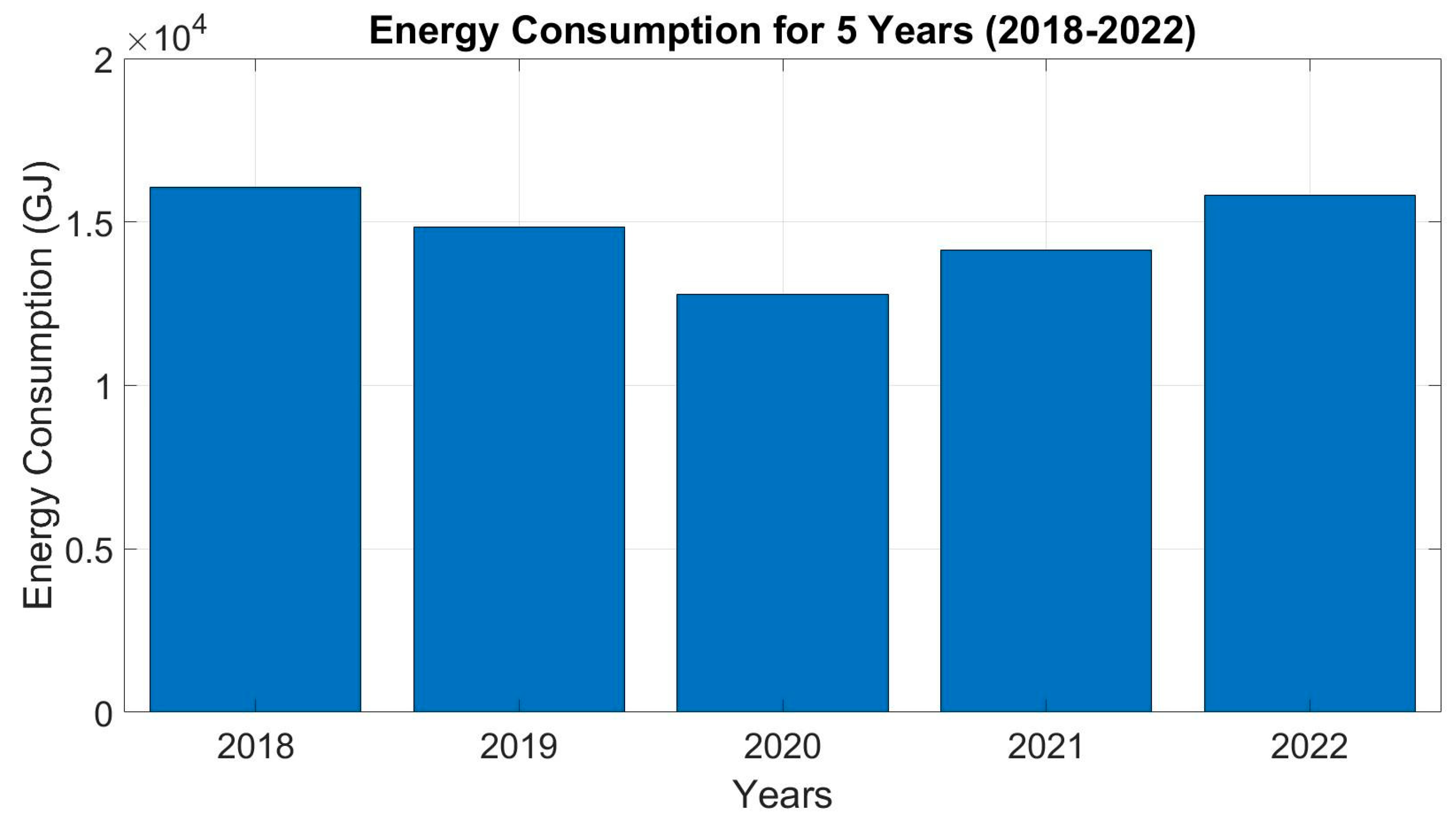
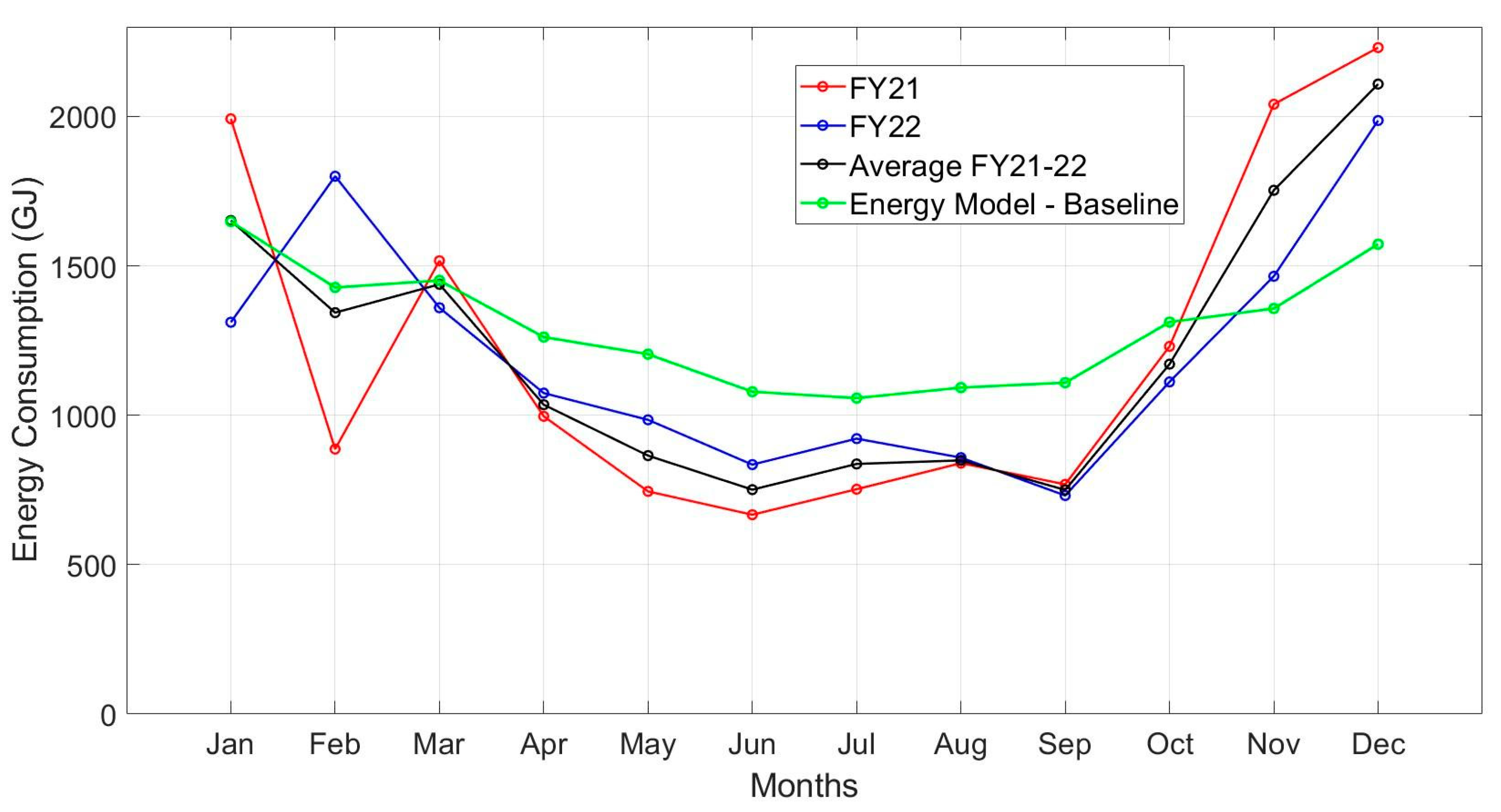
This paper focuses on a light rail maintenance facility audited as part of that project. This facility has an area of 107,000 ft2 (~9941 m2); is located in Baltimore, Maryland; and was constructed in 1991. The facility showed a consistently high energy use intensity (EUI) for five consecutive years, with an average of ~410 kWh/m2. The following four-step procedure evaluated the facility’s energy consumption and performance. First, the building’s performance was analyzed using energy benchmarks and existing utility bills. Once the bills were analyzed, a walkthrough was conducted to identify the deficiencies in the building and ways its performance could be optimized for improved energy efficiency. Step three involved modeling the building’s energy consumption to simulate the baseline energy performance of the facility. The model was based on the building’s original as-built drawings, utility bills, building plug loads, and occupancy schedules. Once the baseline was created and validated, a list of proposed energy efficiency measures (EEMs) was simulated in the energy model. The final step involved documenting the savings in energy, operating costs, and GHG reduction potential that could be achieved by implementing the EEMs. The results show that energy audits of maintenance facilities can produce significant savings. The ramifications of using a four-step approach similar to the one proposed above include the development of a handbook/reference for other facilities that have similar attributes.

2. Facility Energy Performance Assessment

2.1. Building Energy Benchmarking and Utility Bills

Building energy benchmarking involves energy accounting, evaluating opportunities for improvement, and estimating energy and cost savings [25]. By assessing the end-use energy data, facilities’ energy performance can be evaluated using predefined benchmarking metrics, such as CBECS benchmarks [26]. Energy benchmarks are quantified using the fundamental metric of energy use intensity (EUI) measured in kWh/m2 (Equation (1)), which measures a facility’s overall energy consumption over its gross floor area [27]. The other common energy benchmark, the load factor (Equation (2)), is a value that determines the building’s electrical efficiency by comparing the peak demand to the total energy usage in a time frame [28]. As summarized in Table 1, for the maintenance facility, the EUI was ~404 kWh/m2, which is almost three times the CBECS benchmark of ~151 kWh/m2. Additionally, the load factor was calculated to be 0.22, compared to the recommended minimum of 0.75 for moderately efficient buildings. The high EUI and low LF indicate that the maintenance facility is not efficiently using its energy resources. Figure 1 shows the energy consumption profile over the last five years.
E U I   ( E n e r g y   U s e   I n t e n s i t y ) = U t i l i t y   E n e r g y   C o n s u m p t i o n   [ k W h ] F a c i l i t y   S q u a r e   F o o t a g e   [ m 2 ]
L F   ( L o a d   F a c t o r ) = T o t a l   k W h   p e r   p e r i o d P e a k   D e m a n d   ( k W )     N u m b e r   o f   d a y s     24   h o u r s

2.2. Facility Walkthrough

During a facility walkthrough, notes and pictures are taken of all high-energy-consuming devices/equipment as well as building envelope components. The main considerations for the building envelope are places of infiltration, such as windows, doors, garage doors, and other openings. In [29], it was found that infiltration accounted for 6% of total commercial building energy in the U.S. Thus, correcting for infiltration can significantly enhance energy efficiency. The type of materials used and the construction of these features, such as whether windows are single/double-pane or tinted, as well as the number of features present in the building, should be noted during the walkthrough. In addition to the building envelope, high-energy-consuming devices, such as the HVAC system, should be noted. The system’s identification plate should be documented for later reference to the system’s heating/cooling capacities, power rating, efficiency, and critical information. Other significant energy-consuming devices include plug-load equipment for building operation, lighting, and miscellaneous loads found throughout the building’s areas. For this information to be useful, the quantities of each device need to be noted, along with their respective power ratings. Broken devices and equipment should also be considered, as they could lead to less efficient energy consumption. At the end of the walkthrough, the building personnel should be interviewed to gain their perspective on whether the building is operating according to its intended needs. These personnel can provide information on the actual use of some systems compared to the use initially intended from the as-built drawings. The walkthrough and interview allow for the most up-to-date version of the building to be used in the next steps of energy auditing and modeling. Finally, the information transfer from the walkthrough should be aligned to support the implementation of building information modeling [30].

2.3. Energy Model Development

Simulation software allows users to customize libraries according to the nature of the building. The process begins with the construction of the building envelope, where users designate the façade, comprising the walls (interior and exterior walls) and any doors or windows, as well as their performance metrics. Improper material selection at this stage can lead to erroneous baseline building values [31]. Next, the building layout is built into the model, creating a full 3D model of the building with rooms, as shown in Figure 2. To create HVAC zones, rooms can be grouped together and later assigned to specific HVAC equipment, as shown in Figure 3. HVAC equipment can be added, with the significant aspects being heating/cooling size, fan size, variable frequency drive (VFD), and type of system. Once the different HVAC equipment at the maintenance facility is entered into the model, it is added to the appropriate zones. Next, based on the zones, users assign the type of area, which incorporates the typical internal plug loads, heating/cooling loads, occupancy, and lighting. The software also considers the building’s local weather data to simulate outdoor temperatures and the necessary heating and cooling requirements over the course of a year. The flowchart shown in Figure 4 depicts the process of developing a working energy model.

2.4. Identification of Energy-Intensive Areas

Maintenance facilities, depending on their use case and scheduling, can have different energy profiles. In [32], the performance of a railway maintenance facility was optimized by developing the best scheduling policy. Using generic algorithms and industrial simulation software, the facility’s performance was significantly improved. However, an optimized scheduling system cannot be implemented for an MTA maintenance facility due to its 24 × 7 operation schedule. The nature of its operating hours also explains the consistently high EUI for the facility for five consecutive years.
Commercial building energy consumption is divided into four categories: HVAC systems, lighting, equipment (based on building type), and miscellaneous loads [33]. Typically, HVAC systems and lighting comprise 70–75% of a facility’s energy consumption [34]. However, these numbers vary based on building types and their uses. The maintenance facility is a light rail repair facility with washing bay areas, welding shops, vehicle repair floors, fabricating shops, and a multitude of other light rail repair and maintenance services. This comes with various equipment that can increase the plug load and overall base load of the facility. Based on the plug-load inventory provided by the facility manager, some of the most power-intensive equipment in the facility is shown in Table 2.
As seen from Table 2, the facility has a significant plug load that can ramp up the energy consumption for the facility. As this equipment can be complex to model, an overall plug-load density (kW/m2) was applied to the areas where the loads are situated. Each piece of equipment was mapped to its location to develop the most accurate model for the facility’s baseline performance. As 85% of the facility comprises maintenance areas, the facility has high ceilings to accommodate the light rail cars. Therefore, running the system fan continuously is suggested, even when the heating or cooling cycles are off [35]. Continuous air circulation aids in mixing cool and warm air and keeps temperatures in rooms with a high ceiling relatively consistent.

Generalized Energy Efficiency Strategies

As seen in Table 1, the average load factor for the maintenance facility for 2022 was 0.22, leaving tremendous room for improving the facility’s electrical efficiency. In [36], the authors studied the effects of varying the plug-load schedules using an energy monitoring mobile app, and upon implementation, a net 21% reduction in the plug loads in three buildings was achieved. For plug loads such as computers, coffee machines, and fax machines, their control can be easily achieved using smart power strips [37]. However, this approach is unsuitable for monitoring and controlling the equipment list mentioned in Table 2. Therefore, we recommend a common energy conservation measure (ECM), which involves scheduling high-power-rated devices for night/after hours to avoid peak demand charges and simultaneously ameliorate the load factor of the facility [38]. This helps reduce energy demand during peak hours and, consequently, high demand charges. The peak demand charges for maintenance facilities can rise to as high as 5 USD/kW during peak hours [39].
Once the operation of the plug loads was optimized, we turned to methods for managing the HVAC and lighting for the high ceilings. Providing the desired number of lumens for facilities with large ceilings can be complicated. In [40], the lighting performance of commercially available tubular daylight devices (TDDs) under various conditions was experimentally evaluated. It was found that light levels increased, and energy use decreased with solar altitude and TDD diameter. Using a similar approach, we recommended the installation of TDDs to reduce the load of artificial lighting and maximize the benefits of daylight. The specific diameter of the TDDs installed would need to be designed based on the desired lumens for the space [40].
For heating, the maintenance facility mainly uses infrared gas heaters. Infrared gas radiant heaters typically have a higher upfront equipment and installation cost; however, the operating costs of gas heaters are less than electric heaters owing to the higher energy density of natural gas [41]. While these radiant heaters are economically viable and cheaper to run, they increase on-site CO2 emissions, increasing their carbon footprint. In [42], an innovative solution for heat recovery from exhaust gases of ceramic infrared heaters is presented, which allows for environmental benefits and fuel savings in existing buildings heated with radiant heaters with low radiant efficiency. Using a flue gas–water heat exchanger, heat can be extracted from exhaust gases and transferred to water, which can then be used for domestic hot water (DHW) preparation. The maintenance facility has many infrared radiant gas heaters that could be used for heat recovery for hot water preparation. This use of waste heat would increase fuel savings on low-efficiency radiant heaters.

2.5. Advantages of Simulation Software

Simulation software offers a high level of customization, which suits the many different types of systems and zones found in maintenance facilities [43]. Additionally, the report generated for the simulation gives insight into the optimum sizing of the HVAC systems, indicating areas where energy needs are not being met and calculating net energy consumption for a fiscal year. The maintenance facility model was generated for the fiscal year 2022, during which data were actively collected and could be compared for accuracy. Moreover, 2022 is widely regarded as the “post-COVID” benchmark year [44], thereby giving insight into how the facility fared in its energy consumption pre-, during, and post-COVID-19. The model simulation obtained approximately the same energy usage of natural gas and electricity as the collected data. However, there was a slight overestimation of energy use in the summer months and, in the winter months, an underestimation, as shown in Figure 5.
Figure 5 shows the model’s ability to predict the facility’s baseline. An energy model should emulate the facility’s performance so that it can be used to analyze the building’s energy consumption further and develop EEMs. The quality of an energy model relies heavily on professional experience, user judgment, and the quality of inputs provided for model accuracy. Variables in building energy consumption, such as building use, occupancy rates, plug loads, and other sources, can lead to significant differences between the predicted energy use from a model and the actual consumption, thus necessitating calibration. Two statistical indices, the mean error (ME, Equation (3)) and the coefficient of variation of root mean square error (CVRSME, Equation (4)), have been widely used for evaluating the model performance, as recommended by the American Society of Heating, Refrigerating, and Air-Conditioning Engineers [45]. To develop an energy model that replicates the energy performance of a facility, [46] found that the facility’s metered energy consumption values need to lie within the metered consumption of the year being simulated (2022), the preceding year (2021), and the average of the two years. Furthermore, ASHRAE Guideline 14—2014 prescribes no more than 15% and 10% deviation in monthly and annual data, respectively [45]. The maintenance facility energy model fell within these tolerance limits, validating the approach and the model’s accuracy in replicating the building’s energy performance. Thus, the simulated values were close enough to justify the model’s use for developing EEMs for the facility and for predicting the energy savings potential across a year.
M P E = i = 1 j S i M i S i
C V R M S E = i = 1 j ( S i M i ) 2 / j S
S and M are the actual and modeled energy use, respectively, and j is the total number of data recorded (the size of j is 12 for the monthly simulation and 8760 for the hourly simulation). In this case, only monthly data are considered for validation. Table 3 shows the values for the mean error and CVRMSE prescribed by ASHRAE and the corresponding values for our energy model.
Owing to the high plug load, 24 × 7 occupancy and HVAC system operations, and equipment-heavy machinery in the maintenance facility, the values simulated by the energy model were deemed good enough to emulate the facility’s performance.

3. Proposed Energy Efficiency Measures (EEMs)

Many energy efficiency improvements were identified to ameliorate the facility’s subpar energy performance and adhere to the state’s energy efficiency [6] and decarbonization [7] goals. In [47], the effect of single-system retrofits versus integrated packages of energy efficiency measures (EEMs) was evaluated to investigate the overall energy efficiency improvements. Fifteen out of thirty-four case studies implemented single-system retrofits, while the remaining focused on integrated packages. The study found that integrated approaches achieved more than 20% energy savings, while single-system approaches achieved approximately 10% energy savings. This prompted us to evaluate the effect of multiple EEMs on the facility’s overall energy efficiency. The proposed EEMs in this section were formulated based on the major deficiencies existing in the facility.

3.1. LED Lighting Upgrades

A combination of compact fluorescent lamps (CFLs), metal halide, high-pressure sodium, and incandescent lamps provides all maintenance facilities with lighting. All the lighting fixtures have lower lighting power densities (LPD) than LEDs, requiring higher power to provide the same number of lumens and increasing the facility’s energy consumption. Table 4 shows the lighting inventory of the maintenance facility.
In [48], a life-cycle analysis of LED retrofits was performed by replacing traditional artificial lighting in facilities. According to the study, the lifetime of all LED retrofits is longer than the lifetimes of the traditional lamps they are replacing. The study found that T8 and T5 fluorescent lamp replacements with LEDs may yield as much as 40–50% overall savings. For this reason, we modeled the energy savings that could be achieved by replacing the existing lighting with LEDs. In our model, the existing lighting fixtures were replaced with recessed LEDs with wattage based on the lighting power density prescribed by [49].

3.2. Equipment Sizing and Decarbonization

HVAC equipment uses a significant amount of energy while affecting occupant comfort. In recent years, ventilation code requirements have often driven the size of the equipment upward, resulting in mismatched cooling capacities. Oversized cooling equipment experiences shorter run cycles, reducing the ability to dehumidify air and the equipment’s life span [50]. The selection of HVAC equipment can have a significant impact on the overall efficiency and operating costs of the installed system [51]. The maintenance facility faces a similar plight, with oversized equipment driving up energy consumption and costs. Table 5 shows the existing HVAC equipment in the facility and the amount by which it is oversized.
As evident from Table 5, the HVAC systems in the maintenance facility are massively oversized, resulting in egregious energy consumption patterns and significant costs to the facility. Additionally, the heating ventilators and rooftop units (RTUs) use natural gas for heating, increasing the on-site carbon emissions of the facility. With the Environmental Protection Agency (EPA) instituting a penalty on every metric ton of CO2 emitted annually (51 USD/metric ton) [52], facilities need to start looking at their carbon footprint to mitigate the fines that may be imposed on them.
To alleviate the preceding problems, we modeled systems with appropriate HVAC sizing to match the heating and cooling demands of the facility year-round. A 25% margin was added to ensure that the systems are still operational and provide heating and cooling to the facility’s occupants in the event of extreme weather conditions [53]. To ensure further optimal operation of the systems, we modeled the installation of variable frequency drives (VFDs) on all motors above 5 HP, which was found to be economically feasible and have lower payback periods [54]. VFDs would modulate the operation of the compressors and fans in the HVAC systems based on occupancy levels and local temperature settings at the zone level from thermostats. Finally, all the HVAC systems were modeled to use electricity as the sole utility for both heating and cooling. This was carried out to ensure the facility’s ambition to adhere to Maryland’s net-zero goals. Building decarbonization can transform HVAC systems and, consequently, allow facility managers and building owners to promote more efficient and cleaner operations [55].

3.3. Solar PV Installation

The maintenance facility has an available roof area of ~5644 m2, upon which rooftop solar PV could be installed to replace the facility’s grid energy consumption with solar energy. For the developed energy model, the efficiency of the photovoltaic arrays was assumed to be 18%, with an inverter efficiency of 96%. In [56], some of the important tradeoffs were highlighted between the costs and benefits of installing rooftop solar panels for higher energy generation. One tradeoff identified was a marginal increase in energy generation compared to the investment to install higher efficiency solar panels. The study further explored the impact of covering the entire roof area and the corresponding increase in the number of photovoltaic arrays required to achieve this; it was found that to provide the last 3% coverage, 20% more panels would be needed, thereby creating a funding burden. From the results of the study, it was concluded that using 50% of the available rooftop area for solar PV would be a good starting point for the facility while maintaining existing rooftop HVAC systems and skylights. The tilt angle for the photovoltaic arrays was set to 30° to match the latitude of the location and harness maximum energy generation potential [56].

3.4. Temperature Setbacks

The maintenance facility has a 24 × 7 occupancy schedule owing to the maintenance work being carried out in the facility year-round. The existing temperature setpoints for the facility are 75 °F (23.9 °C) year-round, regardless of the ambient temperature or occupancy levels. In [57], it was revealed that the ambient temperature and occupancy can change the EUI of a facility by 7–15%, making it an attractive opportunity for energy savings. It was thus recommended to use temperature setbacks for the facility to produce extra energy and cost savings. However, upon speaking with the facility managers, it was found that the only spaces with fixed occupancy levels were the offices, while the rest of the spaces were used 24 × 7, thereby limiting the scope of temperature setbacks. The office spaces in the facility, which account for 15% of the facility’s overall square footage, were modeled for temperature setbacks based on [58], as seen in Table 6. The occupied temperature setpoint was maintained at 75 °F (23.9 °C), and the unoccupied temperature setpoint was 85 °F (29.4 °C) and 65 °F (18.3 °C) in the summer and winter months, respectively, for the office areas from 9 a.m. to 5 p.m. Over the weekends, the spaces were maintained at the temperature setback setpoints as there was no occupancy.

3.5. Window Replacement

The U-value and solar heat gain coefficient (SHGC) of windows have an enormous impact on buildings’ heating and cooling loads. The U-value measures how well a window insulates, while the SHGC measures how much of the sun’s heat comes through the window. In [59], it was found that the annual heating and cooling energy demand decreased by 8–17% when the U-value of the windows in a poorly insulated house was enhanced, and that demand decreased by 18–30% when the SHGC was lowered for a well-insulated house with larger windows. Furthermore, for buildings in the north-central climate, it is advised to have double-pane windows with a U-factor lower than 0.3 and an SHGC lower than 0.4 [60]. The maintenance facility has single-pane windows original to the building, far beyond their useful life. For the reasons above, it is recommended to replace the existing windows in the facility with double-pane windows with an U-factor ≤ 0.3 and SHGC ≤ 0.4 to reduce the heating and cooling demands of the facility.

4. Results and Discussion

The energy model aims to determine the potential financial savings that could be generated by implementing the recommended EEMs in the maintenance facility. The case studies show that the EEMs can produce substantial energy savings under different scenarios. The results discussed below show the effect that each EEM would have on the overall energy usage of the building and provide explanations and justification for the simulated values.
The proposed EEMs from Section 3 emphasize the implementation of retrofitting existing equipment in the facility with energy-efficient alternatives. Energy-efficient retrofits often have advanced technologies and features that can enhance performance and functionality. In [61], the authors used a multi-criteria decision analysis including location, climate, and operational and embodied energy, but not limited to architectural constraints, control, and management from a life cycle analysis perspective. They found that retrofitting the building envelope, lighting fixtures, and HVAC equipment can be an effective energy efficiency solution. Building energy retrofits provide substantial opportunities to reduce the level of building energy consumption, thereby saving money, improving comfort levels, and reducing greenhouse gas emissions [62]. Furthermore, implementing energy efficiency retrofits also results in upgraded functionality, improved structural and architectural quality, reduced energy consumption, decreased CO2 emissions, and improved indoor air quality [63]. However, the above studies also acknowledge that cost–benefit analyses, including payback periods, must be considered to determine the efficacy of retrofit measures.

4.1. LED Lighting Upgrades Savings

The maintenance facility relies on a mixture of light bulbs, including fluorescent, incandescent, high-pressure sodium, and metal halide. Replacing all lighting with LED equivalents was the first EEM suggested for the facility because, as shown in Table 4, many inefficient lighting fixtures currently illuminate the facility, contributing to high energy consumption. Switching the lighting from the current types was modeled using presets that consider the heat transferred to the surrounding air, efficiency, and other factors. The user defines inputs, including the lighting densities, wattages, and use, based on the area type and schedules. The resulting energy savings predicted by the model were a decrease of 54 MWh/year of electricity and an increase of 54 GJ/year of natural gas.
The reason behind the decrease in electricity values is that LEDs operate at least 75% more efficiently than the currently installed bulbs [64]. However, they release less heat during operation, which explains the rise in therms/year: the natural gas must provide more heating in the building during the winter months to supplement the lower heat gain from lighting.

4.2. Decarbonization Savings: Resizing HVAC, VFDs, and Electrification

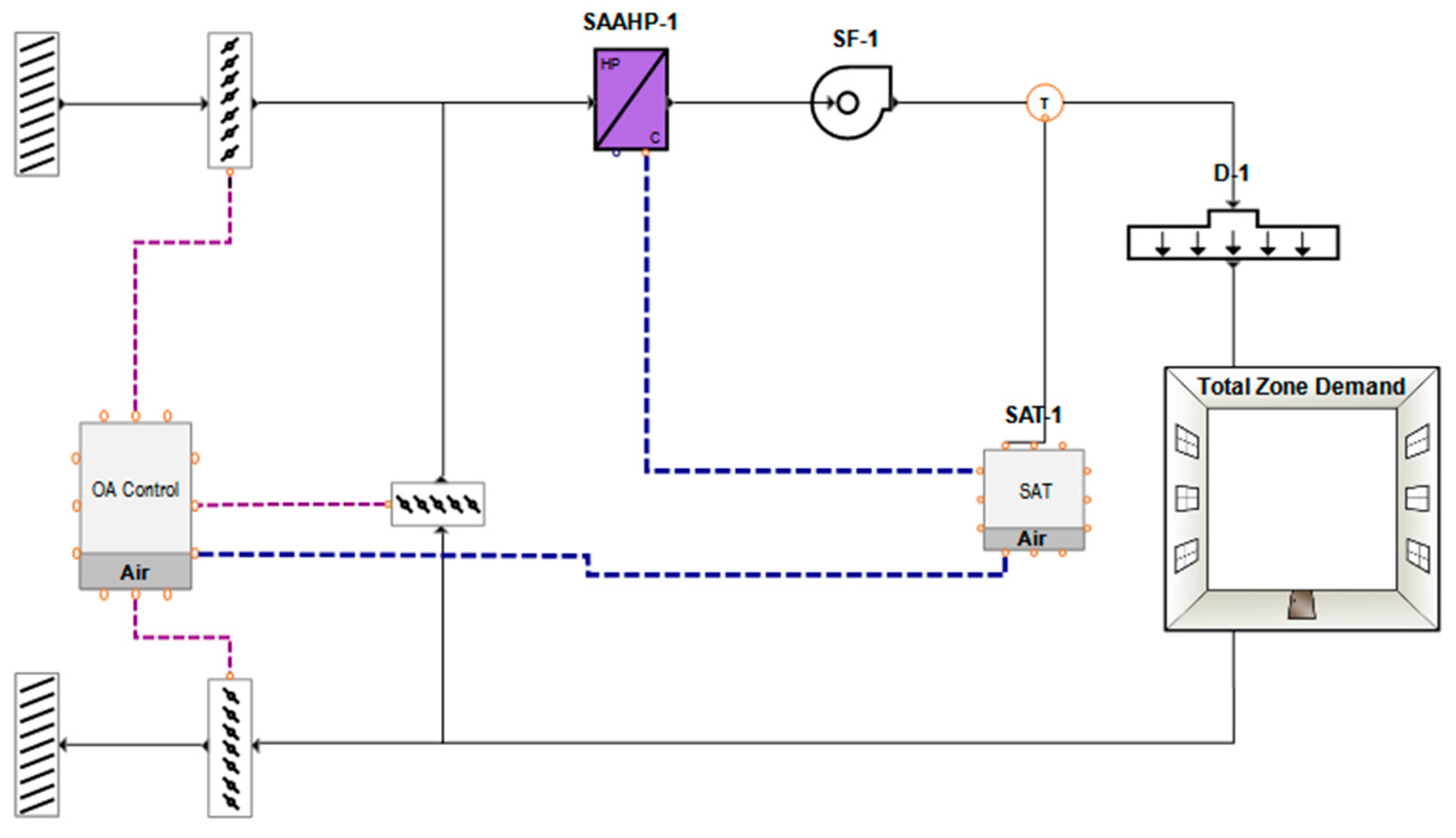
The model allows users to simulate changes in the energy sources of HVAC systems, from electric, gas, and steam to electricity. An example of such a system is depicted in Figure 6. For the various HVAC systems at the maintenance facility, the natural gas components were converted to electrical equivalents, VFDs were applied to any motors over 5 HP, and the HVAC equipment was resized to match the simulated weather loads better. Additionally, adding VFDs to the configuration with the current components was possible. Finally, another option permits the auto-sizing of HVAC equipment. This auto-sizing feature allows the software to determine the worst-case scenario for heating and cooling based on the geographical zones. Combining these three portions into the decarbonization recommendations could achieve savings of 62 MWh/year of electricity and 5034 GJ/year of natural gas. Additionally, the potential annual savings of USD 49,763 and 272 metric tons of CO2 could be achieved.
The ramifications of decarbonizing buildings, starting with HVAC systems, are tremendous in achieving net-zero operations for facilities. HVAC systems are the most energy-consuming systems, consuming approximately 50% of the end energy use in the building sector [65]. Optimizing their use can result in significant savings, both in terms of energy and cost, as well as GHG emissions [66].
The natural gas usage at the facility was eliminated when the HVAC systems were converted to electrical equivalents. As a result, the electrical usage at the facility will increase. However, adding auto-sizing and VFDs in the same simulation counteracted this increased electricity usage and produced a net decrease in electricity use.

4.3. Solar PV Installation

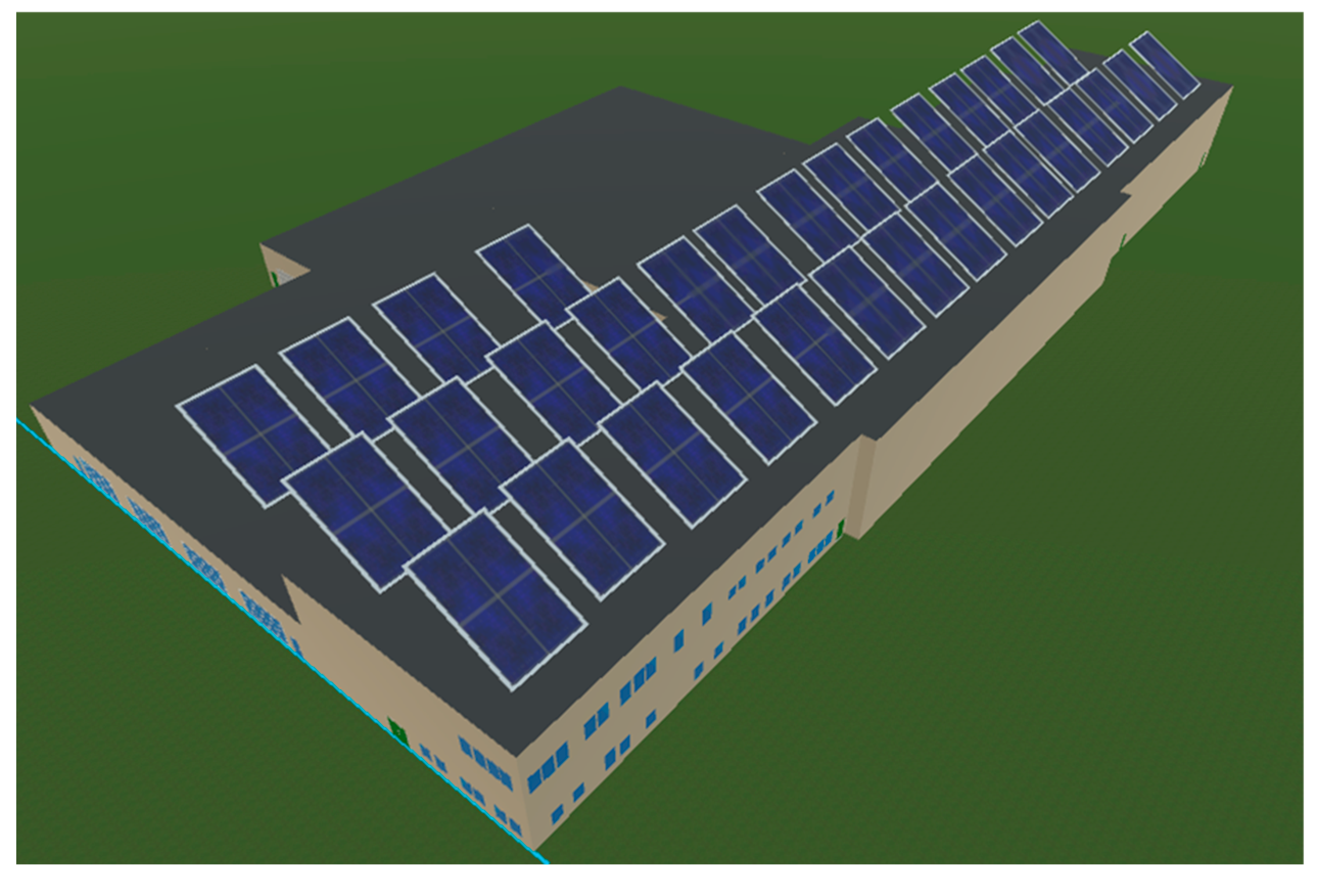
Solar power is intended to supplement the electricity that would be used from the utility supply. A 50% estimation of the total roof area at the maintenance facility was used to determine the useful roof area for installing solar panels. An azimuth angle of 180° and a tilt angle of 30° were the chosen configurations of the solar PV arrays. With the specifications shown below in Figure 7, it is shown that 50 total arrays were needed. The simulated solar array is projected to reduce electricity consumption by 980 MWh/year.
This electricity savings accounts for around 33% of the facility’s energy consumption in the base model. The solar panels did not have any energy storage capability in the simulation, so it was assumed that the energy that was produced directly supplemented the energy from utility sources, i.e., the energy generated by the solar array was sold back to the grid to offset the electricity costs. It was also assumed that the arrays followed net metering by selling surplus power generated while applying credit at the retail rate. Installing energy storage equipment could increase the savings potential of the facility by allowing for energy supplementation during fluctuations, such as peak demand [67].

4.4. Temperature Setbacks

Temperature setbacks at the maintenance facility were recommended for the office area because it operates on a Monday–Friday, 9 a.m. to 5 p.m. schedule. When the office is unoccupied, the temperature is increased or decreased for energy efficiency. The previous temperature setpoint was 75 °F (23.9 °C) year-round for the offices. While that temperature should be maintained when the offices are occupied, the drift point in the winter should be set to 65 °F (18.3 °C) and 85 °F (29.4 °C) in the summer. To implement this new schedule into the software, a new occupancy schedule had to be generated based on the typical 9 a.m. to 5 p.m., Monday–Friday work schedule. In the new schedule, during the winter months, the temperature is set to 75 °F (23.9 °C) when the office area is occupied and drifts to 65 °F (18.3 °C) when unoccupied. Similarly, for the summer, the temperature when occupied is set to 75 °F (23.9 °C), and unoccupied drift is 85 °F (29.4 °C). When building areas are not occupied at all during the day, such as on weekends, the temperature is set to the drift point for the respective season for the full day. When switching from the unoccupied to the occupied temperature set points, the software starts the temperature change an hour before occupants enter the building (8 a.m.) and changes back to the drift temperature an hour after occupants leave (6 p.m.). This new schedule would result in a decrease in electricity use of 6 MWh/year. Temperature setbacks are an important energy-saving measure in the context of energy efficiency, with savings reaching as high as 30% for heating systems and 23% for cooling systems [68].

4.5. Window Replacement

The maintenance facility features windows in the office area, which is only a fraction of the overall building’s square footage. As there have been no window renovations since the original construction of the maintenance facility, it was assumed that the windows are over 30 years old. Given the windows’ age, they were assumed to be typical single-pane windows for the Zone 4 climate zone. The recommended replacement windows should fit North Central Climate Zone standards with an SHGC ≤ 0.40 and U-factor ≤ 0.25 [69]. The replacement windows chosen in the model are double-pane tinted windows with an air-filled gap that meets the required SHGC and U-factor values described above. These upgrades to the existing windows would reduce electricity use by 0.5 MWh/year and increase natural gas use by 316 MJ/year. While the savings are not significant, it should also be noted that the facility does not have many windows that could benefit from the savings from window retrofits. Moreover, the uncertainty in the estimations makes it challenging to gauge whether a retrofit would be economically viable or suffer from high payback periods [70].
Table 7 highlights the energy and cost savings that could be achieved by implementing the EEMs suggested in this study. The utility savings (USD) were calculated using the standard utility rates obtained from the facility’s utility bills. The electricity and natural gas rates were 0.11 USD/kWh and 0.9 USD/MJ, respectively. With the existing prices, it is no surprise that the facility would be averse to all-electric for its operations, owing to the higher energy density of natural gas/dollar invested [71]. By implementing the combination of EEMs for the facility, it was observed that the EUI decreased from 403.7 to 283.6 kWh/m2, a reduction of almost 30%. By electrifying the facility, the peak demand did go up owing to all of the facility’s power being supplied by electricity, but the reduced electricity consumption did aid in an improved load factor of 0.41, an improvement of 86%. While the improvements highlighted are significant, it was noted that the facility would need to continue improving its overall performance to adhere to the state’s goals of energy efficiency and decarbonization.
As seen in Table 7, five different energy efficiency measures (EEMs) were considered for the maintenance facility to improve its energy performance. A final simulation was carried out to investigate the impact of implementing all EEMs simultaneously in the facility and the associated energy savings. It was observed that maximum savings could be achieved with EEMs 2 and 3 by appropriately sizing the equipment and electrifying the existing fossil fuel equipment, along with installing a rooftop solar PV array. While installing the solar PV array can provide significant savings for on-site electricity consumption by virtue of net metering, the GHG reduction in Scope 3 emissions can make for an attractive investment. From Table 5, it can be observed that most of the HVAC equipment in the facility is oversized, causing massive energy waste and associated utility costs. Appropriately sizing HVAC equipment can lead to a good balance between supply and demand for energy consumption for the facility’s use case. Moreover, electrifying the equipment would reduce Scope 1 and Scope 2 emissions from on-site fossil fuel usage. EEMs 1, 4, and 5 were simulated. While the savings from them were not attractive, a combined retrofit for lighting followed by envelope upgrades and temperature setbacks can further improve the facility’s energy efficiency.
Table 8 shows the reduction in GHG emissions that can be achieved by the EEM implementations. Using the coefficients of CO2 equivalents from the EPA Power Profiler [72], the quantity of GHG emissions quantified in metric tons of CO2 from electricity was calculated. The CO2 equivalents for natural gas were obtained from the EPA’s Emission Factors Hub [73].
The highest GHG emission reductions are seen for EEM 2: solar PV installation. However, while analyzing the reductions (energy and GHG emissions) for each utility, the highest reductions for natural gas are observed for EEM 3: equipment sizing and electrification. The maintenance facility uses electricity and natural gas for its operation, with natural gas comprising an annual average of 27% of the total energy consumption and electricity making up the rest. For 2022, the natural gas consumption for the maintenance facility is 3971 GJ, costing USD 33,858, with total GHG emissions of 215 metric tons. Similarly, for 2022, the electricity consumption for the maintenance facility is 2907 MWh, costing USD 241,097, with total GHG emissions of 978 metric tons. Using the rates from [39], it is evident that in the facility’s quest towards net-zero carbon emissions, the most prudent measure would be to decarbonize the HVAC systems and replace them with their electrified counterparts. With non-compliance penalties for on-site emissions being instituted starting in 2030 [7], facilities should start prioritizing reducing on-site Scope 1 and 2 emissions to avoid hefty penalties.

5. Conclusions

The built environment significantly impacts GHG emissions due to its high energy consumption. Although newly constructed buildings are increasingly being built as net-zero facilities, most existing buildings were not built with energy efficiency as a high priority, hence the need to find ways to retrofit existing buildings to achieve global decarbonization and sustainability goals.
The present case study focused on a maintenance facility used by the State of Maryland Mass Transportation Agency. This facility was chosen because the energy performance metrics were below the desired standard benchmark values for comparative facilities. Based on a virtual as well as hands-on energy audit, the recommended EEMs included LED lighting upgrades, the installation of solar PVs, appropriate equipment sizing, the installation of VFDs, window upgrades, temperature setbacks, and electrification measures. These recommendations are projected to offer significant energy savings potential, with a net annual reduction of 584 metric tons of CO2, a decrease of 5034 GJ of natural gas consumption, and 1086 MWh of electricity for 2022. The comprehensive energy audit analysis and simulation models were crucial in identifying deficiencies and opportunities to improve the facility’s performance. Furthermore, the energy modeling results show that implementing the energy efficiency measures has an attractive cost-saving potential of USD 162,402 annually.
The results of this case study show that attractive energy savings can be achieved for a commercial maintenance facility despite having extreme operational schedules. The study also highlights the importance of energy use optimization to enhance building energy efficiency and promote sustainable practices. The outcomes of this study not only contribute to cost and energy savings for the building’s occupants but also serve as a blueprint for future energy reduction optimization projects in similar maintenance facilities. The study aims to serve as a guide for measures that can most benefit other similar maintenance facilities.

Author Contributions

Conceptualization, J.H., A.R., R.F. and M.O.; methodology, J.H. and A.R.; validation, J.H., A.R. and R.F.; data curation, J.H. and A.R.; resources, J.H., A.R. and R.F.; writing—original draft preparation, J.H., A.R.; writing—review and editing, J.H., A.R., R.F. and M.O.; visualization, J.H. and A.R.; supervision, J.H., A.R., R.F. and M.O.; project administration, R.F. and M.O.; funding acquisition, M.O. All authors have read and agreed to the published version of the manuscript.

Funding

The authors declare no competing financial interests. This research was funded in part by the Office of Energy Sustainability within the State of Maryland’s Department of General Services (DGS).

Data Availability Statement

The original contributions presented in the study are included in the article, further inquiries can be directed to the corresponding author.

Acknowledgments

The authors would like to thank the Office of Energy Sustainability within the State of Maryland’s Department of General Services (DGS) for their support of this project.

Conflicts of Interest

The authors declare no conflicts of interest.

References

  1. EIA. (n.d.-a). Frequently Asked Questions (FAQs)—U.S. Energy Information Administration (EIA). Available online: https://www.eia.gov/tools/faqs/faq.php?id=77&t=11 (accessed on 23 November 2023).
  2. Cresko, J.; Rightor, E.; Carpenter, A.; Peretti, K.; Elliott, N.; Nimbalkar, S.; Liddell, H. DOE Industrial Decarbonization Roadmap; No. DOE/EE-2635; USDOE Office of Energy Efficiency and Renewable Energy (EERE): Washington, DC, USA, 2022. [Google Scholar]
  3. van Bommel, N.; Höffken, J.I. The urgency of climate action and the aim for justice in energy transitions–dynamics and complexity. Environ. Innov. Soc. Transit. 2023, 48, 100763. [Google Scholar] [CrossRef]
  4. U.S. Energy Information Administration—EIA—Energy Facts Explained. U.S. Energy Facts Explained—Consumption and Production—U.S. Energy Information Administration (EIA). April 2023. Available online: https://www.eia.gov/energyexplained/us-energy-facts/ (accessed on 23 November 2023).
  5. Allouhi, A.; El Fouih, Y.; Kousksou, T.; Jamil, A.; Zeraouli, Y.; Mourad, Y. Energy consumption and efficiency in buildings: Current status and future trends. J. Clean. Prod. 2015, 109, 118–130. [Google Scholar] [CrossRef]
  6. Governor Moore Signs Executive Order Doubling Maryland’s Energy Conservation Goal through State Government Greenhouse Gas Reductions; Press Releases—News; Office of Governor Wes Moore: Annapolis, MD, USA, 2023.
  7. MDE. The Maryland Climate Solutions Now Act; Maryland Department of Environment (MDE): Baltimore, MD, USA, 2022. [Google Scholar]
  8. Berardi, U. Building energy consumption in US, EU, and BRIC countries. Procedia Eng. 2015, 118, 128–136. [Google Scholar] [CrossRef]
  9. Kontokosta, C.E.; Spiegel-Feld, D.; Papadopoulos, S. The impact of mandatory energy audits on building energy use. Nat. Energy 2020, 5, 309–316. [Google Scholar] [CrossRef]
  10. Deru, M.P.; Deru, M.P.; Kelsey, J. Procedures for Commercial Building Energy Audits; American Society of Heating, Refrigerating, and Air-Conditioning Engineers: Atlanta, GA, USA, 2011. [Google Scholar]
  11. Ian Shapiro, P. Energy audits. ASHRAE J. 2009, 15, 18–27. [Google Scholar]
  12. Kneifel, J. Life-cycle carbon and cost analysis of energy efficiency measures in new commercial buildings. Energy Build. 2010, 42, 333–340. [Google Scholar] [CrossRef]
  13. Mangano, G.; De Marco, A. The role of maintenance and facility management in logistics: A literature review. Facilities 2014, 32, 241–255. [Google Scholar] [CrossRef]
  14. Gao, H.; Koch, C.; Wu, Y. Building information modelling based building energy modelling: A review. Appl. Energy 2019, 238, 320–343. [Google Scholar] [CrossRef]
  15. Kamel, E.; Memari, A.M. Review of BIM’s application in energy simulation: Tools, issues, and solutions. Autom. Constr. 2019, 97, 164–180. [Google Scholar] [CrossRef]
  16. Elnabawi, M.H. Building information modeling-based building energy modeling: Investigation of interoperability and simulation results. Front. Built Environ. 2020, 6, 573971. [Google Scholar] [CrossRef]
  17. Li, W.; Zhou, Y.; Cetin, K.; Eom, J.; Wang, Y.; Chen, G.; Zhang, X. Modeling urban building energy use: A review of modeling approaches and procedures. Energy 2017, 141, 2445–2457. [Google Scholar] [CrossRef]
  18. Mustafaraj, G.; Marini, D.; Costa, A.; Keane, M. Model calibration for building energy efficiency simulation. Appl. Energy 2014, 130, 72–85. [Google Scholar] [CrossRef]
  19. Feng, D.; Yu, Q.; Sun, X.; Zhu, H.; Lin, S.; Liang, J. Risk assessment for electrified railway catenary system under comprehensive influence of geographical and meteorological factors. IEEE Trans. Transp. Electrif. 2021, 7, 3137–3148. [Google Scholar] [CrossRef]
  20. Liu, Z.; Song, Y.; Gao, S.; Wang, H. Review of Perspectives on Pantograph-Catenary Interaction Research for High-Speed Railways Operating at 400 km/h and above. IEEE Trans. Transp. Electrif. 2023. [Google Scholar] [CrossRef]
  21. Song, Y.; Lu, X.; Yin, Y.; Liu, Y.; Liu, Z. Optimization of Railway Pantograph-Catenary Systems for Over 350 km/h Based on an Experimentally Validated Model. IEEE Trans. Transp. Electrif. 2024. [Google Scholar] [CrossRef]
  22. Fu, L.; Chen, Y.; Zhang, M.; Chen, X.; Shen, B. Multifunctional Superconducting Magnetic Energy Compensation for the Traction Power System of High-Speed Maglevs. Electronics 2024, 13, 979. [Google Scholar] [CrossRef]
  23. Ramnarayan, A.; Sarmiento, A.; Gerami, A.; Ohadi, M. An Energy Consumption Intensity Ranking System for Rapid Energy Efficiency Evaluation of a Cluster of Commercial Buildings; ASHRAE Transactions 129; ASHRAE: Atlanta, GA, USA, 2023. [Google Scholar]
  24. Harish, V.S.K.V.; Kumar, A. A review on modeling and simulation of building energy systems. Renew. Sustain. Energy Rev. 2016, 56, 1272–1292. [Google Scholar] [CrossRef]
  25. Building Energy Use Benchmarking. Energy.Gov. August 2022. Available online: https://www.energy.gov/scep/slsc/building-energy-use-benchmarking (accessed on 23 November 2023).
  26. Scofield, J.H. Energy star building benchmarking scores: Good idea, bad science. In ACEEE Summer Study on Energy Efficiency in Buildings; ACEEE: Washington, DC, USA, 2014; pp. 267–282. [Google Scholar]
  27. Vaisi, S.; Firouzi, M.; Varmazyari, P. Energy benchmarking for secondary school buildings, applying the top-down approach. Energy and Buildings 2023, 279, 112689. [Google Scholar] [CrossRef]
  28. Cerna, F.V.; Coêlho, J.K.; Fantesia, M.P.; Naderi, E.; Marzband, M.; Contreras, J. Load Factor Improvement of the Electricity Grid Considering Distributed Energy Resources Operation and Regulation of Peak Load. Sustain. Cities Soc. 2023, 98, 104802. [Google Scholar] [CrossRef]
  29. Ng, L.C.; Dols, W.S.; Emmerich, S.J. Evaluating potential benefits of air barriers in commercial buildings using NIST infiltration correlations in EnergyPlus. Build. Environ. 2021, 196, 107783. Available online: https://www.sciencedirect.com/science/article/abs/pii/S0360132321001906?via%3Dihub (accessed on 23 November 2023). [CrossRef]
  30. Atiba, O.E.; Efemwenkiekie, U.K.; Olatunji, R.O.; Ohunakin, O.S.; Adelekan, D.S.; Oyeleke, O.A. Walk-through energy audit of an institutional building. J. Phys. Conf. Ser. 2019, 1378, 032051. [Google Scholar] [CrossRef]
  31. Alzoubi, H.H.; Al-Zoubi, A.H. Assessment of building façade performance in terms of daylighting and the associated energy consumption in architectural spaces: Vertical and horizontal shading devices for southern exposure facades. Energy Convers. Manag. 2010, 51, 1592–1599. [Google Scholar] [CrossRef]
  32. Hani, Y.; Amodeo, L.; Yalaoui, F.; Chen, H. Simulation based optimization of a train maintenance facility. J. Intell. Manuf. 2008, 19, 293–300. [Google Scholar] [CrossRef]
  33. Pérez-Lombard, L.; Ortiz, J.; Pout, C. A review on buildings energy consumption information. Energy Build. 2008, 40, 394–398. [Google Scholar] [CrossRef]
  34. Sezgen, O.; Koomey, J.G. Interactions between lighting and space conditioning energy use in US commercial buildings. Energy 2000, 25, 793–805. [Google Scholar] [CrossRef]
  35. Kim, G.; Schaefer, L.; Lim, T.S.; Kim, J.T. Thermal comfort prediction of an underfloor air distribution system in a large indoor environment. Energy Build. 2013, 64, 323–331. [Google Scholar] [CrossRef]
  36. Hafer, M.; Howley, W.; Chang, M.; Ho, K.; Tsau, J.; Razavi, H. Occupant engagement leads to substantial energy savings for plug loads. In Proceedings of the 2017 IEEE Conference on Technologies for Sustainability (SusTech), Phoenix, AZ, USA, 12–14 November 2017; pp. 1–6. [Google Scholar]
  37. Nakazawa, F.; Soneda, H.; Tsuboi, O.; Iwakawa, A.; Murakami, M.; Matsuda, M.; Nagao, N. Smart power strip network and visualization server to motivate energy conservation in office. In Proceedings of the 2011 9th IEEE International Conference on Industrial Informatics, Lisbon, Portugal, 26–29 July 2011; pp. 352–357. [Google Scholar]
  38. Surai, J.; Surapatana, V. Load factor improvement in industrial sector using load duration curves. In Proceedings of the 2014 International Electrical Engineering Congress (iEECON), Pattaya, Thailand, 19–21 March 2014; pp. 1–4. [Google Scholar]
  39. EnergyCAP. EnergyCAP Login. (n.d.). Available online: https://my.energycap.com/ (accessed on 23 November 2023).
  40. Fernandes, L.L.; Regnier, C.M. Lighting and visual comfort performance of commercially available tubular daylight devices. Sol. Energy 2023, 251, 420–437. [Google Scholar] [CrossRef]
  41. Roth, K.; Dieckmann, J.; Brodrick, J. Infrared radiant heaters. Ashrae J. 2007, 49, 72. [Google Scholar]
  42. Dudkiewicz, E.; Fidorów-Kaprawy, N.; Szałański, P. Environmental benefits and energy savings from gas radiant heaters’ flue-gas heat recovery. Sustainability 2022, 14, 8013. [Google Scholar] [CrossRef]
  43. Sustar, J. ASHRAE History of a System: History of Trane’s TRACE™ Software. ASHRAE Trans. 2020, 126, 640–643. [Google Scholar]
  44. Cortiços, N.D.; Duarte, C.C. Energy efficiency in large office buildings post-COVID-19 in Europe’s top five economies. Energy Sustain. Dev. 2022, 68, 410–424. [Google Scholar] [CrossRef] [PubMed]
  45. Guideline ASHRAE. Measurement of energy, demand, and water savings. ASHRAE Guid. 2014, 4, 1–150. [Google Scholar]
  46. Shailza. Energy Modeling of Multi-Storied Residential Buildings—A Manual Calibration. In Proceedings of the ASHRAE Building Performance Analysis Conference, Chicago, IL, USA, 26–28 September 2018. [Google Scholar]
  47. Sherman, R.; Naganathan, H.; Parrish, K. Energy savings results from small commercial building retrofits in the US. Energies 2021, 14, 6207. [Google Scholar] [CrossRef]
  48. Raditschova, J.; Gasparovsky, D. Critical analysis of cost benefits of LED retrofits in indoor lighting. In Proceedings of the 2018 VII Lighting Conference of the Visegrad Countries (Lumen V4), Třebíč, Czech Republic, 18–20 September 2018; pp. 1–6. [Google Scholar]
  49. ANSI/ASHRAE/IES Standard 90.1-2022; Energy Standard for Sites and Buildings Except Low-Rise Residential Buildings. ASHRAE: Atlanta, GA, USA, 2022.
  50. Gorter, J.L. HVAC equipment right-sizing: Occupant comfort and energy savings potential. Energy Eng. 2012, 109, 59–75. [Google Scholar] [CrossRef]
  51. Burdick, A. Strategy Guideline: HVAC Equipment Sizing; National Renewable Energy Lab.(NREL): Golden, CO, USA, 2012. [Google Scholar] [CrossRef]
  52. Sheet, E.F. Social Cost of Carbon; United States Environmental Protection Agency (EPA): Washington, DC, USA, 2013. [Google Scholar]
  53. O’Brien, W.; Abdelalim, A.; Gunay, H.B. Development of an office tenant electricity use model and its application for right-sizing HVAC equipment. J. Build. Perform. Simul. 2019, 12, 37–55. [Google Scholar] [CrossRef]
  54. Aditya, T. Research to study variable frequency drive and its energy savings. Int. J. Sci. Res. IJSR 2013, 2, 253–256. [Google Scholar]
  55. Rumsey, E.; Le Garrec, J.; Levasseur, A. How Building Decarbonization Can Transform HVAC. ASHRAE J. 2021, 63, 14–27. [Google Scholar]
  56. Zhong, Q.; Tong, D. Spatial layout optimization for solar photovoltaic (PV) panel installation. Renew. Energy 2020, 150, 1–11. [Google Scholar] [CrossRef]
  57. Selvacanabady, A.; Judd, K.S. The Influence of Occupancy on Building Energy Use Intensity and the Utility of an Occupancy-Adjusted Performance Metric; Pacific Northwest National Laboratory: Richland, WA, USA, 2017. [Google Scholar]
  58. Szydlowski, R.F.; Wrench, L.E.; ONeill, P.J.; Paton, J.B. Measured Energy Savings from Using Night Temperature Setback; No. PNL-SA-20552; CONF-921021-4; Pacific Northwest Lab.: Richland, WA, USA, 1992. [Google Scholar]
  59. Ahn, B.L.; Kim, J.H.; Jang, C.Y.; Leigh, S.B.; Jeong, H. Window retrofit strategy for energy saving in existing residences with different thermal characteristics and window sizes. Build. Serv. Eng. Res. Technol. 2016, 37, 18–32. [Google Scholar] [CrossRef]
  60. What Makes it ENERGY STAR? EnergyStar. October 2023. Available online: https://www.energystar.gov/products/res_windows_doors_skylights/key-product-criteria (accessed on 23 November 2023).
  61. Fernandes, J.; Santos, M.C.; Castro, R. Introductory review of energy efficiency in buildings retrofits. Energies 2021, 14, 8100. [Google Scholar] [CrossRef]
  62. Shaikh, P.H.; Shaikh, F.; Sahito, A.A.; Uqaili, M.A.; Umrani, Z. An overview of the challenges for cost-effective and energy-efficient retrofits of the existing building stock. Cost-Eff. Energy Effic. Build. Retrofit. 2017, 257–278. [Google Scholar] [CrossRef]
  63. Fasna MF, F.; Gunatilake, S. Energy retrofits to enhance energy performance of existing buildings: A review. In Proceedings of the 8th World Construction Symposium, Colombo, Sri Lanka, 8–10 November 2019. [Google Scholar]
  64. LED lighting. Energy.Gov. August 2021. Available online: https://www.energy.gov/energysaver/led-lighting (accessed on 23 November 2023).
  65. Perez-Lombard, L.; Ortiz, J.; Maestre, I.R. The map of energy flow in HVAC systems. Appl. Energy 2011, 88, 5020–5031. [Google Scholar] [CrossRef]
  66. Vakiloroaya, V.; Samali, B.; Fakhar, A.; Pishghadam, K. A review of different strategies for HVAC energy saving. Energy Convers. Manag. 2014, 77, 738–754. [Google Scholar] [CrossRef]
  67. Amrouche, S.O.; Rekioua, D.; Rekioua, T.; Bacha, S. Overview of energy storage in renewable energy systems. Int. J. Hydrogen Energy 2016, 41, 20914–20927. [Google Scholar] [CrossRef]
  68. Moon, J.W.; Han, S.H. Thermostat strategies impact on energy consumption in residential buildings. Energy Build. 2011, 43, 338–346. [Google Scholar] [CrossRef]
  69. ENERGY STAR® Program Requirements for Residential Windows, Doors, and Skylights. January 2015. Available online: https://www.energystar.gov/sites/default/files/Windows_Doors_and_Skylights_Program_Requirements%20v6.pdf (accessed on 23 November 2023).
  70. Ohlsson, K.A.; Nair, G.; Olofsson, T. Uncertainty in model prediction of energy savings in building retrofits: Case of thermal transmittance of windows. Renew. Sustain. Energy Rev. 2022, 168, 112748. [Google Scholar] [CrossRef]
  71. Brehm, P. Natural gas prices, electric generation investment, and greenhouse gas emissions. Resour. Energy Econ. 2019, 58, 101106. [Google Scholar] [CrossRef]
  72. Environmental Protection Agency. eGRID Power Profiler. EPA, 13 February 2024. Available online: https://www.epa.gov/egrid/power-profiler (accessed on 23 November 2023).
  73. GHG Emission Factors Hub. EPA. February 2024. Available online: https://www.epa.gov/climateleadership/ghg-emission-factors-hub (accessed on 23 November 2023).
Figure 1. Energy consumption profile for the maintenance facility.
Energies 17 01907 g001
Figure 2. A 3D model of the maintenance facility developed using the simulation software.
Energies 17 01907 g002
Figure 3. (a) First floor of the maintenance facility in the simulation software. (b) Second floor of the maintenance facility in the simulation software.
Energies 17 01907 g003
Figure 4. Flow chart of the energy model development.
Energies 17 01907 g004
Figure 5. Simulated maintenance facility energy consumption compared to “FY2021 and 2022”.
Energies 17 01907 g005
Figure 6. Example HVAC system with configurable components.
Energies 17 01907 g006
Figure 7. Model view of the implemented solar PV in the simulation software.
Energies 17 01907 g007
Table 1. Comparison of the maintenance facility’s energy benchmarks against industry standard benchmarks.
Energy Benchmark Maintenance Facility (2022)Benchmark
EUI [kWh/m2] 403.7151.1
Load factor 0.220.75
Table 2. Plug-load inventory for the maintenance facility.
Plug LoadQuantityPower Rating (kW)
Car truck hoist722.5
Wheel truing machine164
Lathe motor231.7
Paint booth system179.8
Wheel press143.2
Bridge crane335
Actual press138.2
Train washer equipment254
Air stripper unit243.2
Table 3. Validation of energy model with ASHRAE Guideline 14—2014.
IndexASHRAE Guideline 14 [45]Energy Model
Mean error (ME)56.3
CVRMSE1517.8
Table 4. Lighting inventory for the maintenance facility.
Lamp TypeNumber of Fixtures
Fluorescent1045
Incandescent4
High-pressure sodium65
Metal halide70
Table 5. Existing equipment size and amount oversized by.
EquipmentCapacity (kW)Oversizing (kW)
Unit Heater-15.03.3
Unit Heater-28.92.9
Unit Heater-35.00.4
Unit Heater-48.92.9
Unit Heater-55.92.9
Unit Heater-629.92.3
Unit Heater-710.02.3
Heat Pump-16.44.5
Heat Pump-26.44.5
Heat Pump-311.48.2
Heat Pump-44.24.0
Heat Pump-53.41.6
RTU-157.940.6
RTU-271.733.9
Heating Ventilator-146.90.0
Heating Ventilator-246.90.0
Heating Ventilator-346.90.0
Heating Ventilator-446.90.5
Heating Ventilator-546.90.0
Heating Ventilator-627.813.5
Heating Ventilator-746.938.0
Table 6. Temperature setpoints in the office areas during occupied and unoccupied periods.
MonthsOccupied Temperature Setpoint °F (°C)Temperature Setback Setpoints °F (°C)
May–September75 (23.9)85 (29.4)
October–April75 (23.9)65 (18.3)
Table 7. Savings from different EEMs for the maintenance facility.
#EEMEnergy ConsumptionProjected Energy SavingsEEM Energy Savings PercentageUtility Savings
E (MWh/yr)NG (GJ/yr)E (MWh/yr)NG (GJ/yr)E (%)NG (%)E (USD/yr)NG (USD/yr)Total (USD/yr)
1LED lighting upgrade2873508854−541.9−1USD 5940−USD 462 USD 5478
2Solar PV194850349800330USD 107,800USD 0USD 107,800
3Equipment sizing and electrification286606250342.1100USD 6820USD 42,943USD 49,763
4Window upgrades292750340.5−0.300USD 55−USD 3USD 52
5Temperature setbacks292250346010USD 660USD 0USD 660
Combined EEMs184201086503437100USD 119,460USD 42,943USD 162,402
Table 8. GHG reduction from EEMs in metric tons of CO2.
#EEMProjected Energy SavingsAnnual GHG Reduction 2022
E (MWh/yr)NG (GJ/yr)E (Metric Tons/yr)NG (Metric Tons/yr)Total (Metric Tons/yr)
1LED lighting upgrade54−5416−314
2Solar PV98002990299
3Equipment sizing and electrification62503419253272
4Window upgrades0.5−0.3000
5Temperature setbacks60202
Combined EEMs10865034331253584
Disclaimer/Publisher’s Note: The statements, opinions and data contained in all publications are solely those of the individual author(s) and contributor(s) and not of MDPI and/or the editor(s). MDPI and/or the editor(s) disclaim responsibility for any injury to people or property resulting from any ideas, methods, instructions or products referred to in the content.

