Abstract
For the energy transition in the residential sector, heat pumps are a core technology for decarbonizing thermal energy production for space heating and domestic hot water. Electricity generation from on-site photovoltaic (PV) systems can also contribute to a carbon-neutral building stock. However, both will increase the stress on the electricity grid. This can be reduced by using appropriate control strategies to match electricity consumption and production. In recent years, artificial intelligence-based approaches such as reinforcement learning (RL) have become increasingly popular for energy-system management. However, the literature shows a lack of investigation of RL-based controllers for multi-family building energy systems, including an air source heat pump, thermal storage, and a PV system, although this is a common system configuration. Therefore, in this study, a model of such an energy system and RL-based controllers were developed and simulated with physical models and compared with conventional rule-based approaches. Four RL algorithms were investigated for two objectives, and finally, the soft actor–critic algorithm was selected for the annual simulations. The first objective, to maintain only the required temperatures in the thermal storage, could be achieved by the developed RL agent. However, the second objective, to additionally improve the PV self-consumption, was better achieved by the rule-based controller. Therefore, further research on the reward function, hyperparameters, and advanced methods, including long short-term memory layers, as well as a training for longer time periods than six days are suggested.
1. Introduction
To achieve the German government’s goal of a climate-neutral country by 2045, the scenario presented by Prognos [1] shows a need for a total of 14 million heat pumps in the building sector. This electrification of the heat supply of buildings is often combined with the installation of a photovoltaic (PV) system on the roof to produce renewable energy on-site [2]. Both the grid consumption of the heat pump and the grid feed-in of the PV system will place a load on the electricity grid that it was often not designed for. However, the need for grid extension can be mitigated by matching electricity demand with on-site generation and peak shaving, both of which reduce the load on the grid. The thermal inertia of the building structure and the thermal storage provide flexibility in the operation of modulating heat pumps by temporally decoupling heat consumption and heat production. Using this flexibility can provide a cheaper alternative or additional flexibility to battery storage [3].
Besides rule-based control strategies, more advanced approaches using model predictive control (MPC) for PV-optimized control of heat pumps have been developed in the past, e.g., Kuboth et al. [4]. However, they require high quality forecasts [5] and cannot be easily implemented due to the high effort of designing and parameterizing each energy system model required for the variety of existing buildings [6].
To overcome these drawbacks, artificial intelligence (AI) approaches have become increasingly popular for building energy-system control in recent years. In their review article [7], Alanne and Sierla discuss the learning ability of buildings at a system level and give an overview of machine-learning (ML) applications for building energy management. A major application of ML is the control of heating ventilation and air conditioning (HVAC) systems.
One of the three types of machine learning that is used for system control is reinforcement learning (RL) [8]. The so-called RL agent learns an optimal control strategy by interacting with the building energy system (environment). It can also learn preferences, such as comfort requirements, by interacting with users. RL is potentially model-free, i.e., unlike the mixed-integer (non)linear programming (MI(N)LP) approaches, which are most commonly used for MPC; there is no need for models of the building energy system. Forecasts for weather and heat/electricity demand are also not required but can be implemented and will improve the results [9,10,11,12].
(Deep) reinforcement learning (D)RL methods have been investigated for the control of a variety of energy (sub)systems in residential buildings. While Yu et al. [10] want to “…raise the attention of SBEM [smart building energy management; author’s note] research community to explore and exploit DRL, as another alternative or even a better solution for SBEM.”, Wu et al. [13] note that reinforcement learning algorithms “…could be promising candidates for home energy management…”.
As the statistics in several publications [9,12,14,15,16] show, the number of publications on (deep) reinforcement learning for building energy-system control has been increasing significantly since approximately 2013.
Vázquez-Canteli and Nagy [9] collected, analyzed, and finally selected 105 articles focusing on RL for demand response (DR), maximizing human comfort, and reducing (peak) energy consumption. They classified the publications according to the type of energy system, RL algorithm, and objective and analyzed whether the approach used a single agent or multiple agents. As one of four major groups of energy systems, heating ventilation and air conditioning and domestic hot water (DHW) systems have been identified as having significant demand response potential. However, many publications on HVAC systems only examine the reduction in thermal-energy demand but not the (flexible) heat production. An energy system that includes an air source heat pump, thermal storage, and a PV system, as described in Section 2, is not examined in any publication.
Mason and Grijalva [17] conducted a comprehensive review of RL for autonomous building energy management (BEM), including HVAC systems, water heaters, and home management systems (HMS) that control a variety of combinations of different appliances or energy subsystems. They identified Q-learning as the most commonly used RL method but also a trend towards DRL algorithms. Due to the trial-and-error nature of learning RL agents, direct application to control a real building energy system would result in unacceptable high initial energy costs and occupant discomfort. Therefore, the authors recommend pre-training the RL agent in simulation.
Wang and Hong [14] provide very detailed statistics on 77 publications that investigate RL for building control. A total of 35.5% of the listed publications have HVAC systems as the subject of control, while only 7.3% focus on thermal energy storage (TES). The former were mostly published between 2015 and 2019, while there is no trend for the latter. Most of the RL methods used are value-based (79.3%); only 12.2% use actor–critic algorithms. None of the reviewed papers consider TES in combination with actor–critic algorithms, which are recommended by Fu et al. [15] for continuous action-space problems. They give an overview of (D)RL methods and their ability to solve specific problems in the field of building control, e.g., with small/large discrete or continuous action spaces, and show statistics on the algorithms used in the reviewed literature. However, Wang and Hong [14] conclude that cross-study comparisons are difficult if not impossible due to different environmental settings and benchmarks used in different investigations. Standardized control problems and integrated software tools that combine machine-learning capabilities and building simulation are proposed to overcome this drawback but are lacking.
Perera and Kamalaruban [16] categorized publications based on seven areas of application of RL approaches, including building energy-management systems. They conclude, among other things, that the lack of use of deep-learning techniques and state-of-the-art actor–critic methods hinders performance improvements.
Yu et al. [11] also provide a comprehensive review of publications on deep reinforcement learning (DRL) for smart building energy management (SBEM), distinguishing between studies on single building energy subsystems, multi-energy subsystems in buildings, and microgrids. Only three publications on single building energy subsystems examine electric water heaters, and another three examine HVAC systems with the primary goal of reducing energy costs or consumption. The rest do not examine residential buildings. Only one of the publications on multi-energy subsystems in buildings [18] examines a system similar to the one used in this paper (Section 2.1). The difference with the system investigated here is the use of an additional backup system of a gas boiler and energy costs as the objective.
Shaqour and Hagishima [12] analyzed a database of 470 publications on DRL-based building energy-management systems (BEMS) for different building types and reviewed recent advances, research directions, and knowledge gaps. Their selection resulted in 31 publications focused on residential buildings, of which only three used thermal energy storage and investigated RL approaches on a single-family home or district level. Zsembinszki et al. [19] investigate a very complex building energy system for a single-family house using two water storage tanks, a phase change material storage tank, and a battery storage to provide flexibility to the energy system. Glatt et al. [20] developed an energy-management system for controlling energy storages of individual buildings in a microgrid using a decentralized actor–critic reinforcement learning algorithm and a centralized critic. Kathirgamanathan et al. [21] designed and tuned an RL algorithm to flatten and smooth the aggregated electricity demand curve of a building district. The latter two used CityLearn as a simulation environment.
Only two publications [5,22] were found that investigate a system configuration identical to the one used in this paper. Ludolfinger et al. [22] developed a novel recurrent soft actor–critic (RSAC) algorithm for energy cost optimized heat pump control and compared it with four RL-based and one simple rule-based approach. However, their studies refer to a single-family house, and the training and simulation of the RL agent were performed only for a winter period of two and one week, respectively. The models were developed in Modelica, and the RL agent was developed in Python. Langer and Volling [5] transformed a mixed-integer linear program (MILP) into a DRL implementation and compared the self-sufficiency achieved by a deep deterministic policy gradient (DDPG) algorithm, a model predictive controller (MPC) under full information (theoretical optimum), and a rule-based approach. However, due to their small system dimensions, the buildings considered in Ye et al. [18] and Langer and Volling [5] are also very energy efficient single-family houses. Their investigations are based on simplified linear models developed in previous MILP investigations with time-step sizes of one hour, where mass flows and temperatures in hydraulic circuits and thermal storages are not considered in detail.
Most of the publications analyzed in the literature review focus on energy-efficient, single-family buildings and are often based on simplified linearized models originally developed for MILP approaches with hourly time resolution. There are no studies on new or renovated multi-family buildings with an energy system including an air source heat pump, thermal storage, and a PV system.
The novelty of this work is, therefore, the investigation of a DRL-based approach (i) to control the energy system of a multi-family building (ii) using a physical model that takes into account mass flows and temperatures in hydraulic circuits and thermal storages in detail, requiring a variable time-step solver due to the complexity of the model. This approach differs from published work using constant time steps, usually one hour, which is too coarse for real heat pump control. For the first time, the MATLAB software environment [23] is used with the three toolboxes: Simulink [24] as development environment; CARNOT [25] for building energy-system modeling; and Reinforcement Learning [26] to design, train, and simulate a (D)RL-based controller for a PV-optimized control of an air source heat pump. The purpose of this paper is to show how four selected DRL algorithms perform in this context by evaluating two objectives and comparing them with rule-based controllers. The first objective is to maintain only the required temperatures in the thermal storage. The second objective is to additionally improve the PV self-consumption and self-sufficiency by shifting heat pump operation to times of PV-surplus.
This paper is structured as follows. In Section 2, the methodology of designing the simulation environment and the controllers is described. The applied building energy system model is introduced, two rule-based control strategies used as a reference are described, and the development of two RL agents, one without and one with PV-optimization, is shown. The training and selection of an RL-based controller as well as the results of annual simulations using (i) the reference rule-based controllers and (ii) the developed RL-based controllers are presented and discussed in Section 3. Section 4 concludes the paper and gives an outlook.
2. Methodology
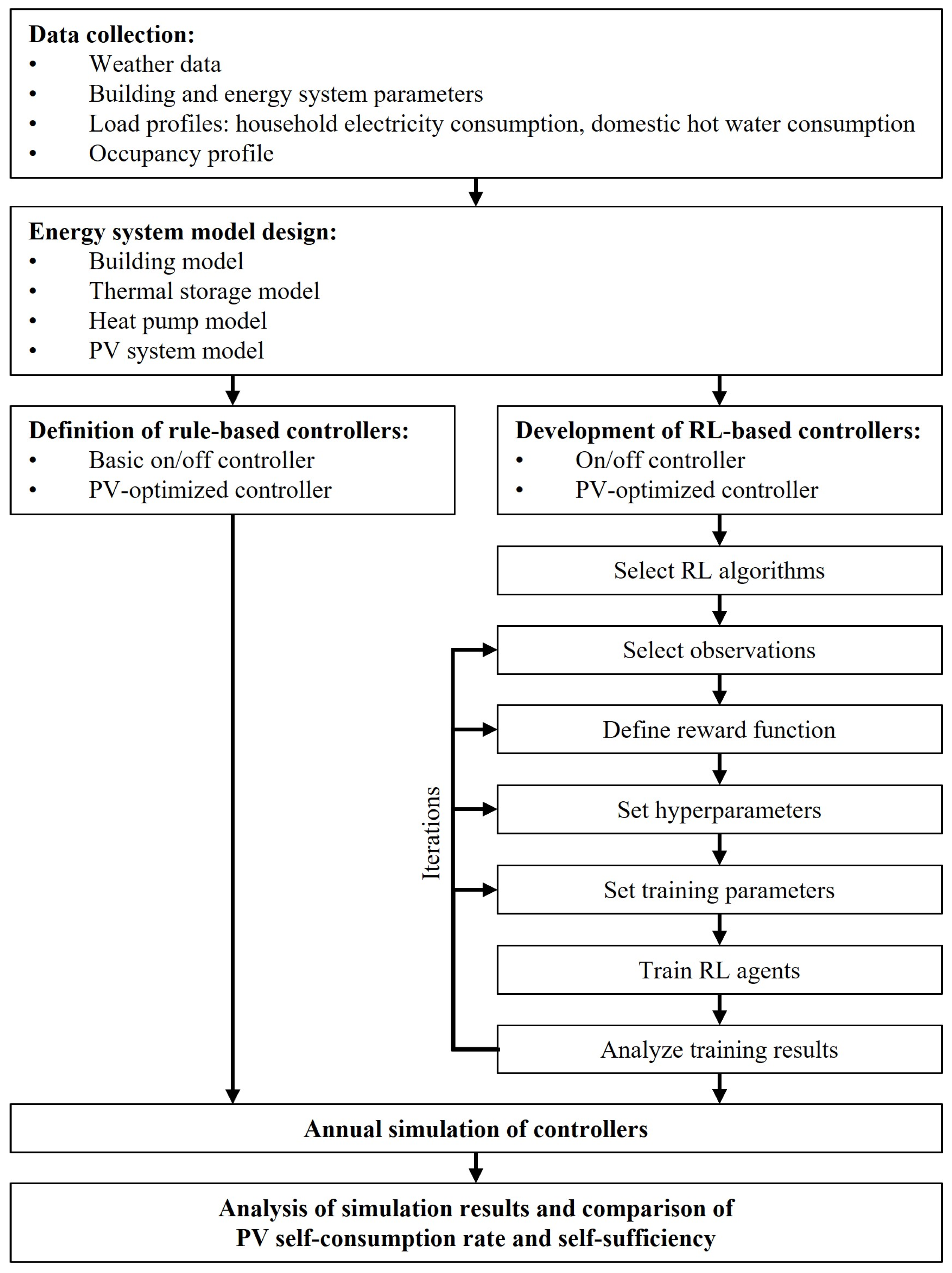
The methodology used for this work is shown in Figure 1.
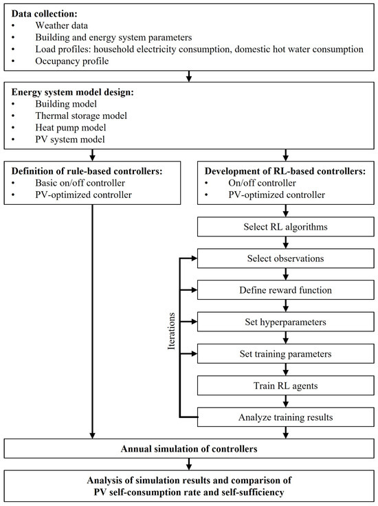
Figure 1.
Methodology of designing the simulation environment and the rule-based and RL-based controllers.
To set up the simulation environment, data and parameters for the building and energy-system model were collected, including load and occupancy profiles and weather data. Based on this data, the sub-models for the building, the thermal storage, the heat pump, and the PV system were created and parameterized (Section 2.1). Due to the modeled mass flows and temperatures in the hydraulic circuits and thermal storage, the complexity of the model and the dynamics, especially for system control, increased compared to simplified linearized models. To solve such problems, very short time steps are required. Therefore, a variable time-step solver was used to reduce the computational effort.
Two rule-based controllers were defined for reference (Section 2.2). The development of the two RL-based controllers (Section 2.3) was an iterative process. First, suitable RL methods were selected, followed by the selection of the observations, the definition of the reward function, and the setting of the hyperparameters and the training parameters. The next step was the training of the RL agents and the analysis of the training results. Based on the success of the training, adjustments of the observations, reward function, hyperparameters, and training parameters were made iteratively until the training results were satisfactory. Finally, the two rule-based and two RL-based controllers were used in an annual simulation. The two PV-optimized controllers were compared to each other by the performance indicators PV self-consumption and self-sufficiency (Section 3).
2.1. Building Energy-System Model
Multi-family buildings account for approximately 41% of the living space in Germany [27] and, therefore, have a large potential for energy savings and flexibility in energy supply. With 19% (225 million m2) of the total living space of multi-family buildings in Germany (1168 million m2), the building age category E of the IWU building typology of Germany [27] is the largest category for multi-family buildings.
A study on multi-family buildings [2] investigated low-energy concepts for energy renovations of multi-family buildings and developed, analyzed, and demonstrated solutions for the efficient use of heat pumps, heat transfer systems, and ventilation systems. They show that heat-supply temperatures can be reduced to 60 °C or less by replacing only a few radiators in critical rooms (e.g., 2–7% of the existing radiators in the cases studied), which makes heat pumps a suitable heat-supply solution in this case. Additionally, the energy consumption of such buildings can be reduced by using electricity from an on-site PV system. According to these results, the conventionally renovated version of the building age category E was selected for the investigations.
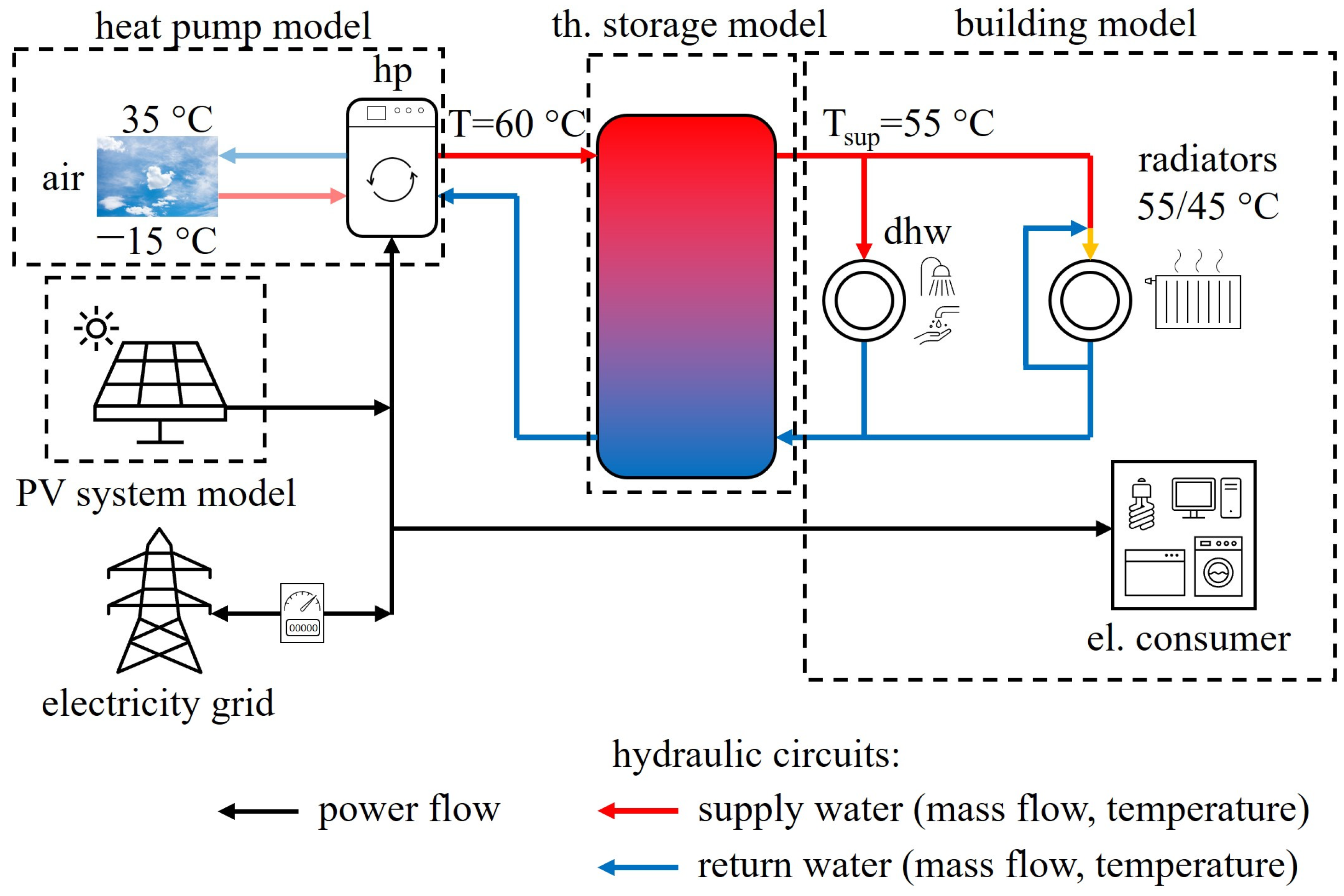
MATLAB [23] and the toolboxes Simulink [24] and CARNOT [25] were used to model the investigated building with its heat and electricity demand and the energy system consisting of an air source heat pump (hp), a thermal storage, and a PV system as shown in Figure 2.
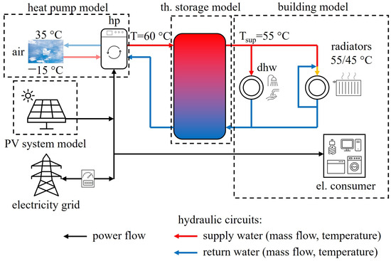
Figure 2.
Investigated building energy system consisting of the electric and thermal consumers (right side), the thermal storage (in the middle), an air-to-water heat pump, and the PV system (left side).
The parameters (geometry, U-values, etc.) of the multi-family building with a heated living space of approximately 2850 m2 divided into 32 apartments were defined according to the data of Loga et al. [27]. To ensure hygienic air exchange, a ventilation system with a constant ventilation rate of 0.4 1/h is included in the building model. According to the user behavior, additional ventilation is used to prevent an overheating of the building in summer. The internal heat gains were defined according to the occupancy profile for residential buildings given in the SIA guideline 2024 [28] and scaled to 60 occupants. As input for the simulations as well as for the load profile generation, the test reference year (TRY) of Ingolstadt provided by the German Weather Service [29] was used. For the generation of the hourly household electricity consumption profile (also used for internal heat gains of electrical appliances) and the domestic hot water (DHW) consumption profile, the method described in the VDI guideline 4655 [30] was used. The annual household electricity consumption was set at 96,000 kWh/a, and the annual DHW consumption was set at 61,500 kWh/a. A stratified thermal storage tank (total volume 8.5 m3) is modeled as a hydraulic separator between the heat pump hydraulic circuit and the consumer hydraulic circuit. It decouples the thermal energy consumption from the heat production, thus providing some flexibility in the operation of the heat pump. A south-facing PV system of 65 kWp is modeled to partially cover the electricity demand of the households and the heat pump. Even in the ideal case of 100% PV self-consumption, 2/3 of the electricity consumed must come from the grid [31]. The dimension of the PV system was derived from an existing building. The building energy-system parameters are summarized in Table 1.

Table 1.
Parameters of building energy system.
2.2. Reference Control Strategies
Two reference rule-based control strategies were defined and used as a reference for the comparison with the RL-based control strategy.
When PV electricity generation is not available or being considered, heat pumps in combination with a thermal storage were often operated in an on/off mode, depending on the temperatures in the thermal storage (basic controller) in former days. In the case shown here, the heat pump is turned on when the top storage temperature drops below 55 °C and runs until the bottom storage temperature reaches that temperature.
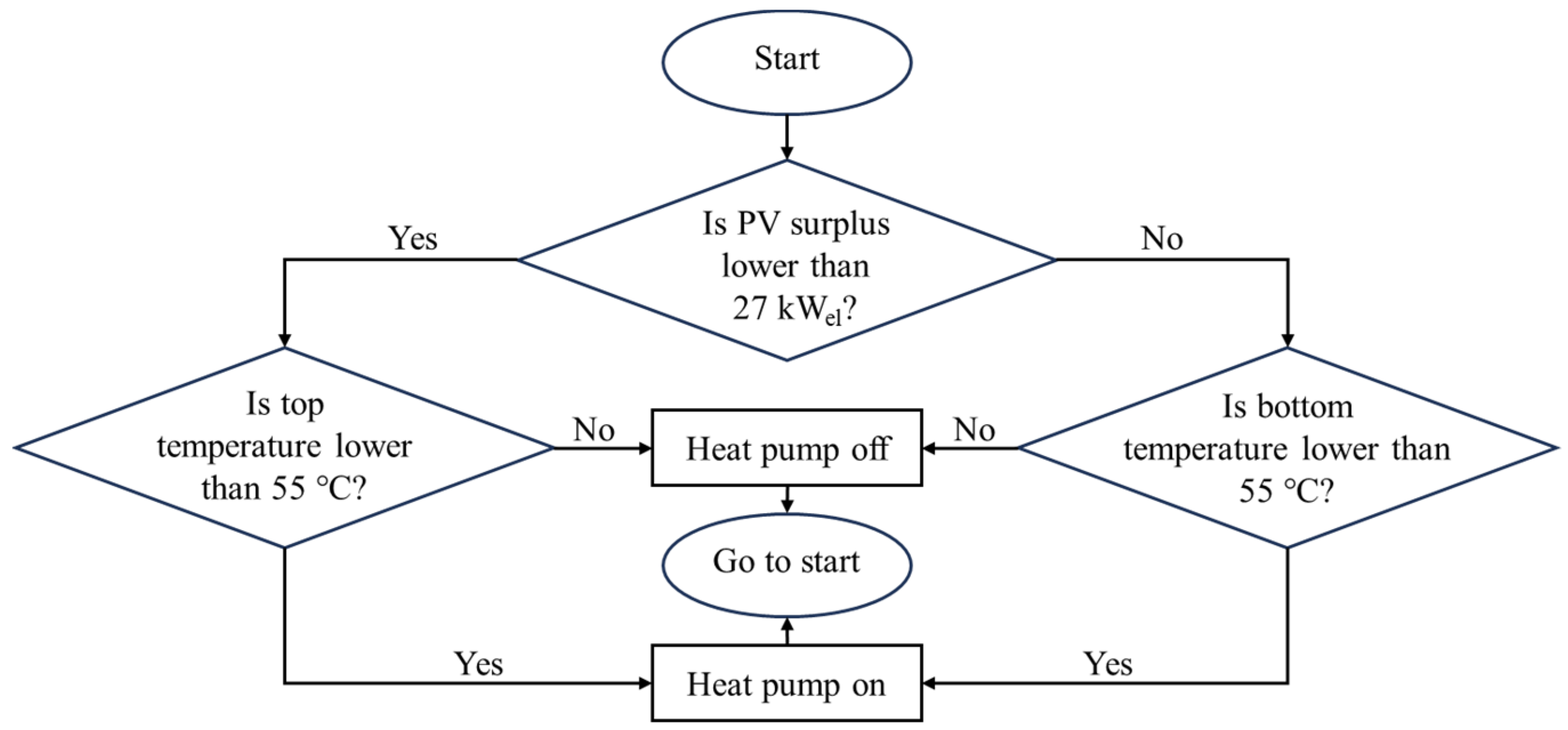
There are several rule-based approaches to better match the heat pump electricity consumption and PV generation, often taking advantage of the modulation of the heat pump. The controller used here (PV-optimized controller) is designed to use most of the PV electricity that is not directly used in the households (PV surplus). If there is no PV surplus, the controller only runs the heat pump to keep the top storage temperature at 55 °C to ensure the heat supply. If the PV surplus exceeds the limit defined by the electricity consumption of the heat pump at the lowest modulation level (27 kWel at 30%), the heat pump is switched on and modulated to consume exactly the PV surplus as long as the bottom storage temperature is lower than or equal to 55 °C. This approach is shown in Figure 3.
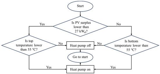
Figure 3.
Flow chart of rule-based, PV-optimized controller.
2.3. Development of Reinforcement Learning-Based Heat Pump Controller
According to the RL Toolbox User’s Guide [32], the workflow for setting up an RL-based controller involves six steps, as shown in Figure 4.

Figure 4.
Workflow of setting up an RL-based controller (according to [32]).
First, the problem to be solved by the RL agent must be defined (step 1). Two objectives are considered in this study. For the first objective, the RL agent controls the heat pump to ensure temperatures of at least 55 °C in the top of the thermal storage to supply heat to the consumers and to avoid temperatures higher than 55 °C, due to the operating limits of the heat pump, and lower than 45 °C in the bottom of the thermal storage. The action of the RL agent is the control signal to the modulating heat pump in a continuous range between 0 and 1, while values lower than 0.3 switch off the heat pump. The actions are based on the observation of the top (Ttop) and bottom storage temperature (Tbottom), the thermal load for space heating and domestic hot water preparation, and the absolute electricity exchange with the grid (Psum). The second objective is extended to a PV optimization. The storage temperatures should be kept within the previously defined range, while the heat pump should run at times when the PV electricity exceeds the household electricity consumption. Therefore, the observations are extended with information such as PV surplus (PPV,surp), PV generation including historical data and forecasts, and time of day and day of the year to allow for the RL agent to learn diurnal and seasonal correlations.
The building energy-system model described in Section 2.1 defines the environment (step 2) with which the agent interacts by giving actions and receiving observations and the reward shown next.
The following two reward functions were defined (step 3) for the two objectives mentioned. Equations (1)–(3) were designed only for keeping the storage temperatures within the defined range:
rt = rtop + rbottom
If the temperatures at the top and bottom of the thermal storage become too low and the temperatures at the bottom become too high, a negative reward is given to avoid such conditions.
Equations (4)–(7) were designed to additionally optimize the heat pump operation to times of PV surplus (PPV,surp). The reward rt for keeping the storage temperatures in the defined range has been slightly adjusted compared to Equations (1)–(3) due to better learning experienced during training.
rel2 = −100a if PPV,surp = 0 kW else 10a
rtotal = rt + rel1 + rel2
In Equation (6), a is the action value (control signal for heat pump) chosen by the RL agent. In the ideal case, there is no electricity consumption from or feed-in into the grid, which results in a positive reward of 5. If there is no PV surplus, the action value a is multiplied by a negative reward of −100 to prevent the agent from choosing high action values that switch on the heat pump charging the thermal storage. In this way, the state of charge of the thermal storage should be kept low until it can be charged by using the PV surplus, which reduces the grid feed-in. This should reduce the amount of power exchanged with the grid, which also increases the PV self-consumption rate.
After the problem is defined, the RL agent can be created (step 4). The RL agent requires a fixed time-step size, which was set to 5 min. Four algorithms were used to train an RL agent:
- Soft Actor–Critic (SAC);
- Twin-Delayed Deep Deterministic (TD3);
- Proximal Policy Optimization (PPO);
- Trust Region Policy Optimization (TRPO).
Based on the results (shown in Section 3.2.1), the algorithm used for validation in an annual simulation (step 6, Section 3.2) was selected for both objectives.
Due to the high computational effort of training an agent (step 5) for an entire year, it was decided to train the agent only for an episode length of one day, randomly chosen from a predefined set of days distributed throughout the year, to avoid overfitting but still represent the characteristics of an entire year. Based on experiences from previous studies [31], a backup controller was implemented in the model. It intervenes and overrides the control signal given by the RL agent when the storage temperatures violate the defined temperature range. This ensures that the agent can explore actions that lead to unintended temperature conditions and learn to avoid them because of the negative reward received. Thus, the backup controller switches the heat pump on if the top temperature falls below 55 °C or switches the heat pump off if the bottom temperature exceeds 57 °C. In both cases, a negative or zero reward is given to the RL agent to make it learn to avoid such conditions.
3. Results and Discussion
This section presents the evaluation of the RL-based controllers and the comparison with the rule-based controllers. First, the results of the annual simulations of the two described rule-based controllers used as a reference are presented, followed by the training results of four RL algorithms and the final selection of an algorithm for the annual simulations. Finally, the results of the annual simulation of the RL-based controllers are discussed.
3.1. Simulation Results of Reference Control Strategies
In the reference case of the temperature-based on/off heat pump controller (basic controller), the households and the heat pump directly consume 48.1% of the PV-generated electricity. Due to the high electricity demand, which is approximately three times higher than the PV electricity generation, the self-sufficiency is only 16.7%, which is very low compared to a net-zero energy single-family building with 37% [33]. But in comparison to single-family buildings with the same ratio of annual electricity consumption and PV-generation of 1/3 and a self-consumption rate of approximately 57% [34], it is very similar. With the rule-based PV optimization of the heat pump operation, both the self-consumption rate and the self-sufficiency can be increased by approximately 15%, as shown in Table 2.

Table 2.
Simulation results of rule-based heat pump control strategies.
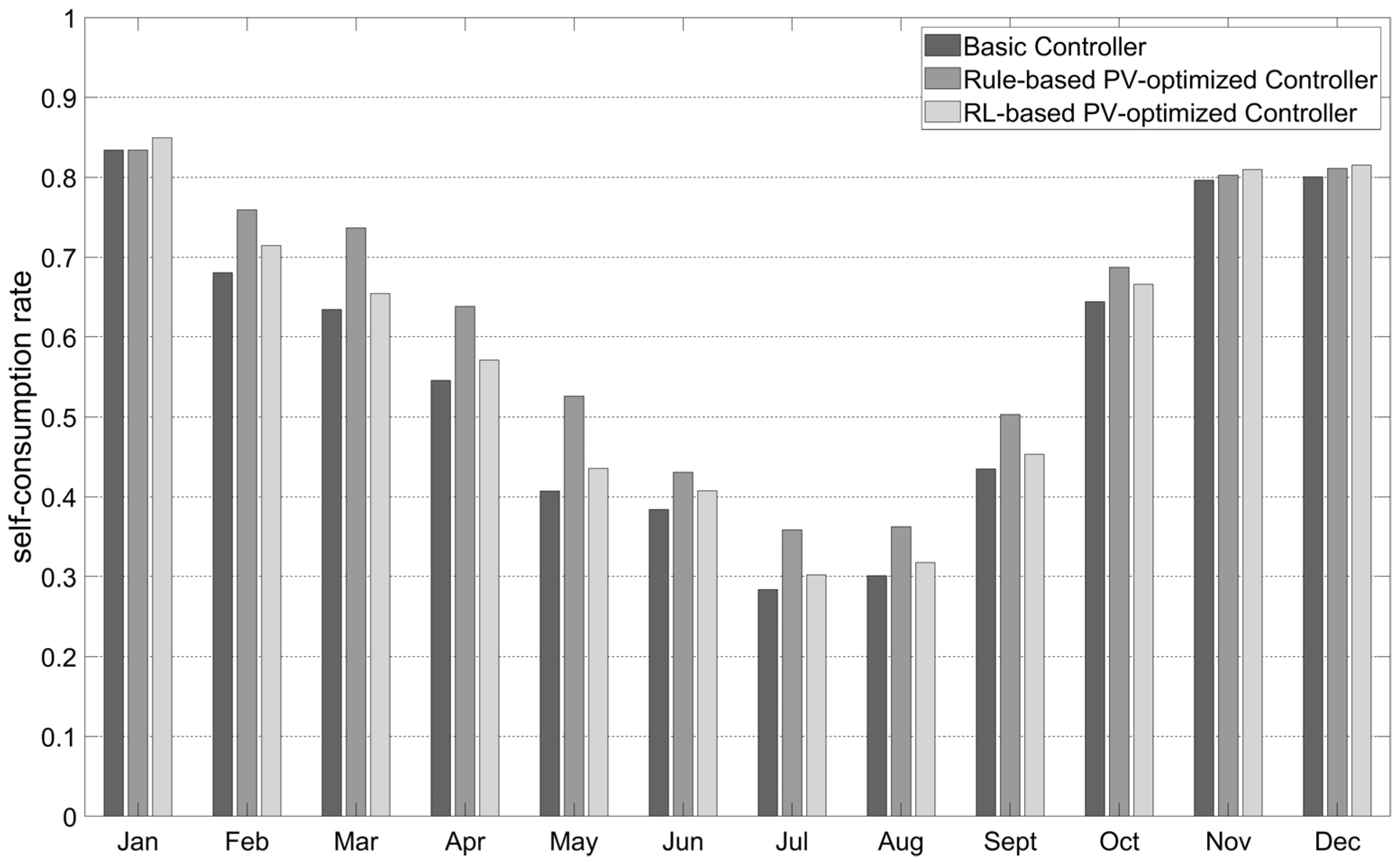
The monthly analysis (Figure 5) shows a maximum self-consumption rate of 84% in January and a minimum self-consumption rate of 28% in July for the basic controller.

Figure 5.
Comparison of monthly self-consumption rates of basic controller, rule-based PV-optimized controller, and RL-based PV-optimized controller.
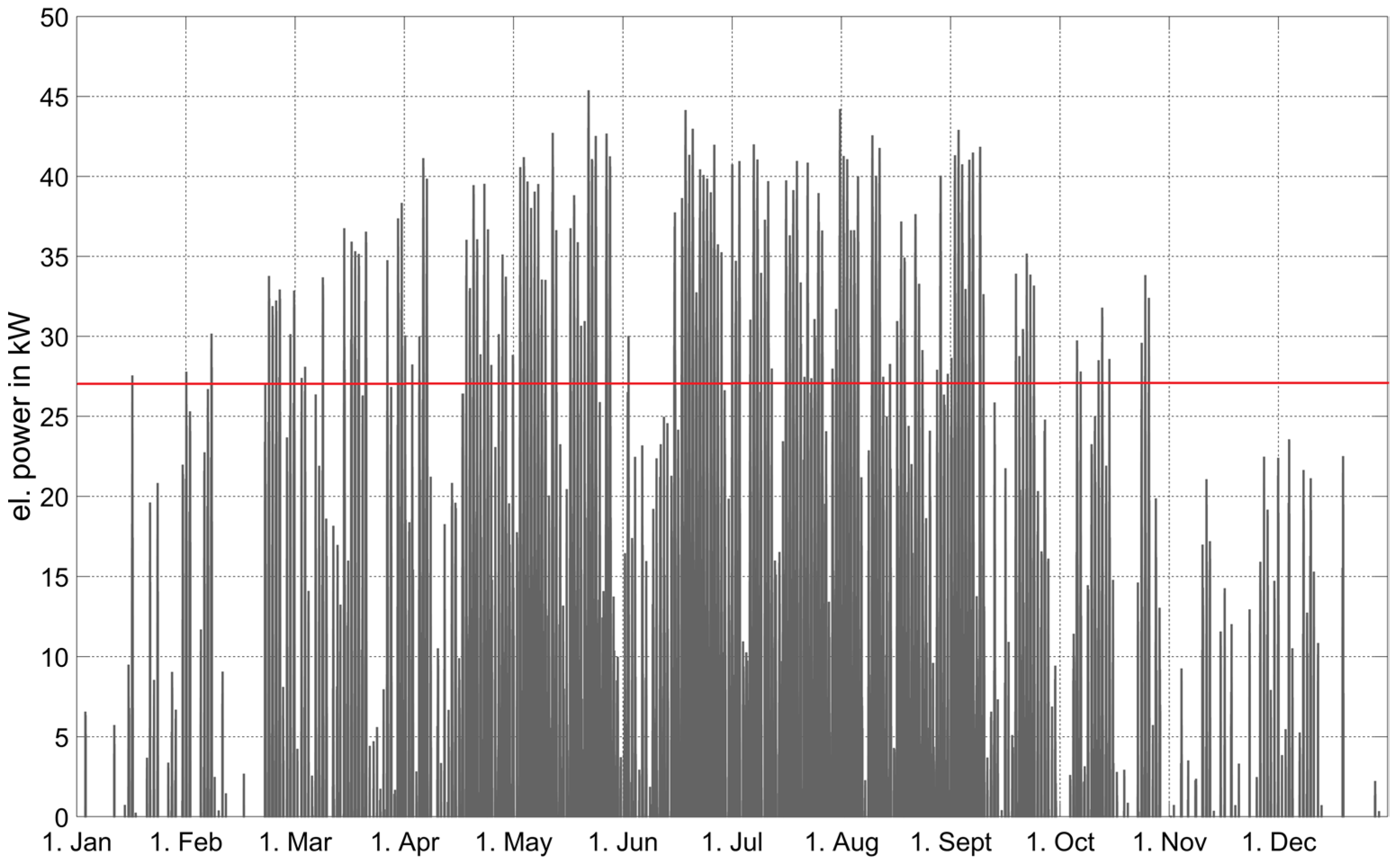
When PV optimization is used, only in transition periods and during the summer, the self-consumption can be significantly increased by up to 29% in May, but there is no improvement in winter. The reason for this is that, in winter, the PV surplus does not reach the minimum electricity consumption of the heat pump of 27 kW as shown in Figure 6, so the heat pump is not switched on to use it. Only approximately 5250 kWh/a of the total 34,900 kWh/a of PV surplus can be used by the heat pump. Thus, there is still potential for a battery storage to better match electricity demand and generation, e.g., by shifting PV electricity from day to night.
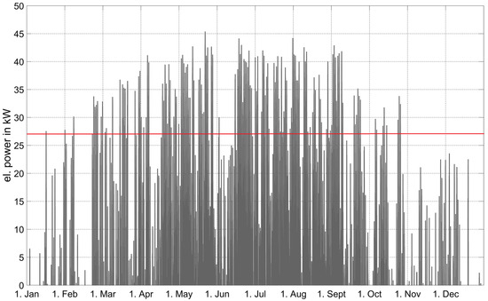
Figure 6.
PV surplus (PV generation minus household electricity consumption) and minimum electricity consumption of the heat pump (red line).
3.2. Simulation of Reinforcement Learning-Based Heat Pump Controller
As previously described, an RL-based approach was tested using the integrated software of MATLAB, and two controllers were developed for operating the heat pump: one to only keep the thermal storage temperatures within the defined range and the other to additionally optimize the heat pump operation to times with PV surplus.
3.2.1. Design, Training, and Selection of RL Agent
To find a suitable RL approach for both objectives, four agents were designed using different RL algorithms with identical hyperparameters (Table 3).

Table 3.
Hyperparameters for RL agent trainings.
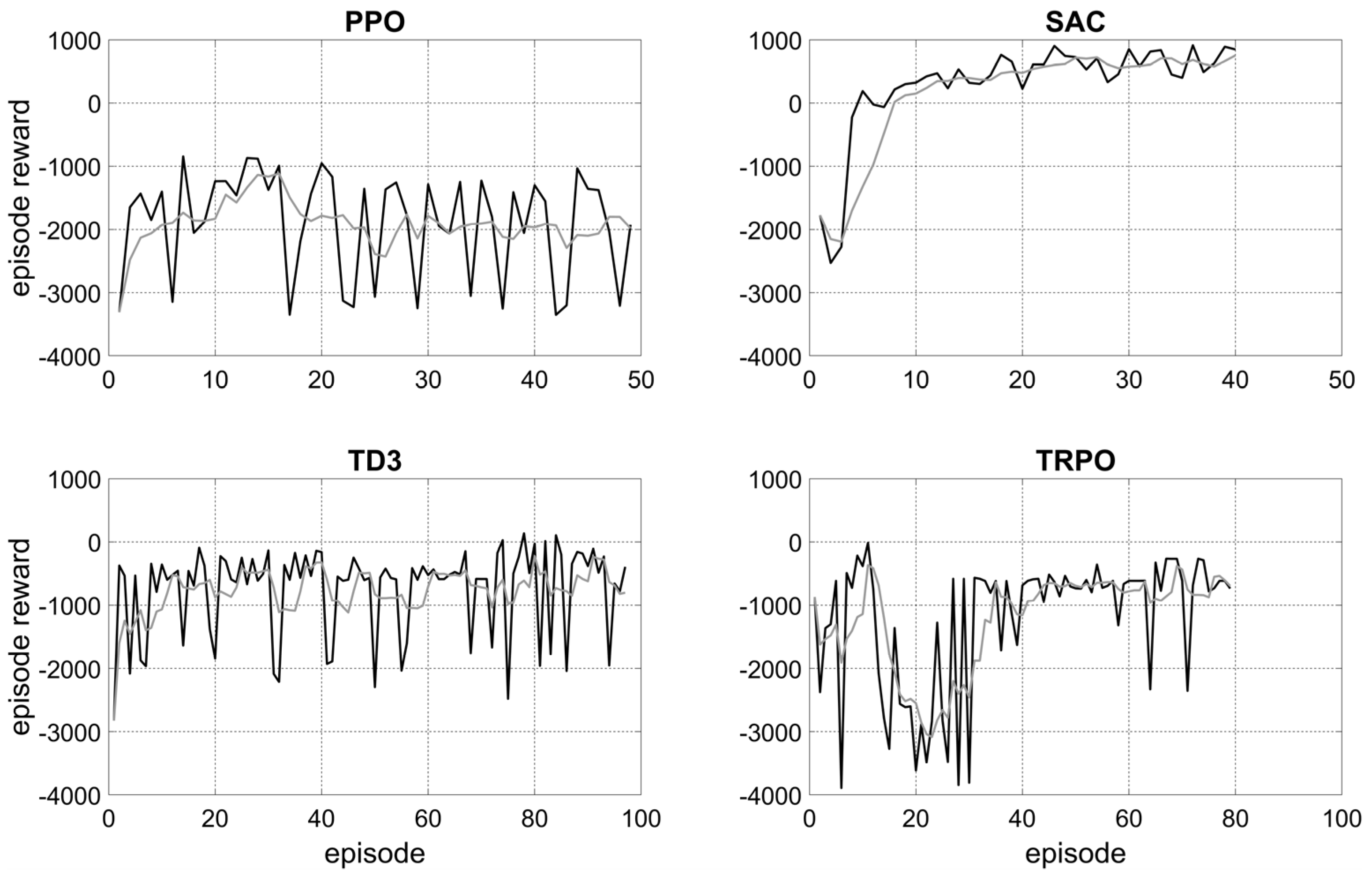
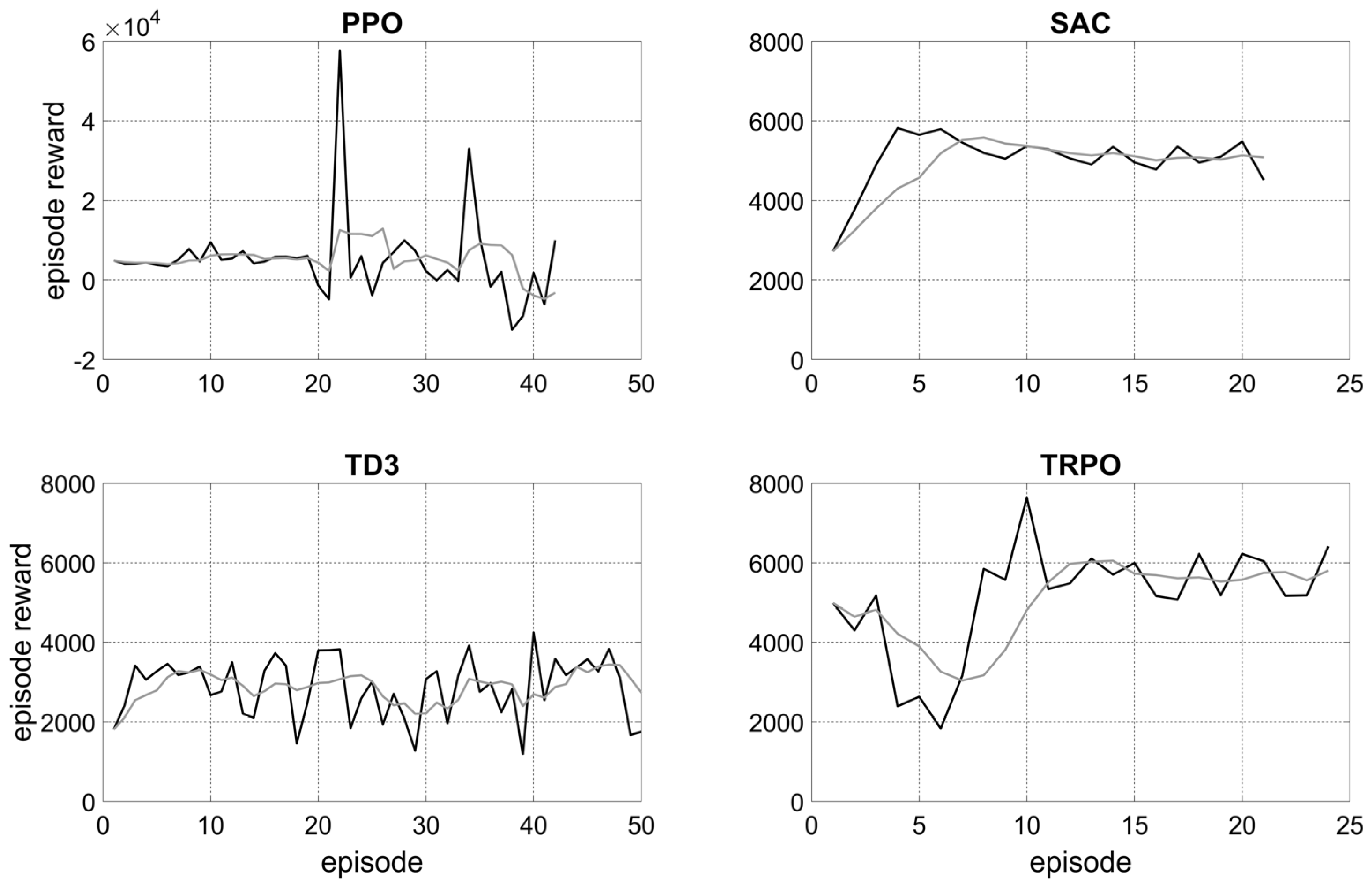
For each agent, training was performed, and the reward obtained, averaged over five episodes, as well as the fluctuation of the episode rewards shown in Figure 7 and Figure 8 were analyzed to determine if the learning process converges. Table 4 and Table 5 compare the average rewards over the last five training episodes between the algorithms used and give an assessment of convergence.
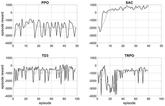
Figure 7.
Episode reward (black line) and average reward over five episodes (grey line) of the training of four RL agents without PV optimization.
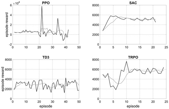
Figure 8.
Episode reward (black line) and average reward over five episodes (grey line) of the training of four RL agents with PV optimization.

Table 4.
Training results of RL agents without PV optimization.

Table 5.
Training results of RL agents with PV optimization.
Convergence was observed for only three trainings. These cases also show the highest average episode rewards. For the agents without PV optimization, the soft actor–critic (SAC) method achieved the best results. For the agents with PV optimization, two methods achieved very good results: the SAC and the trust region policy optimization (TRPO) agent. According to these results, three annual simulations were performed (Section 3.2.2).
However, due to the high sensitivity of the learning process and its computation time to the hyperparameters and the reward function, it may also be possible to achieve better results with the other RL methods when both are adapted.
3.2.2. Simulation Results
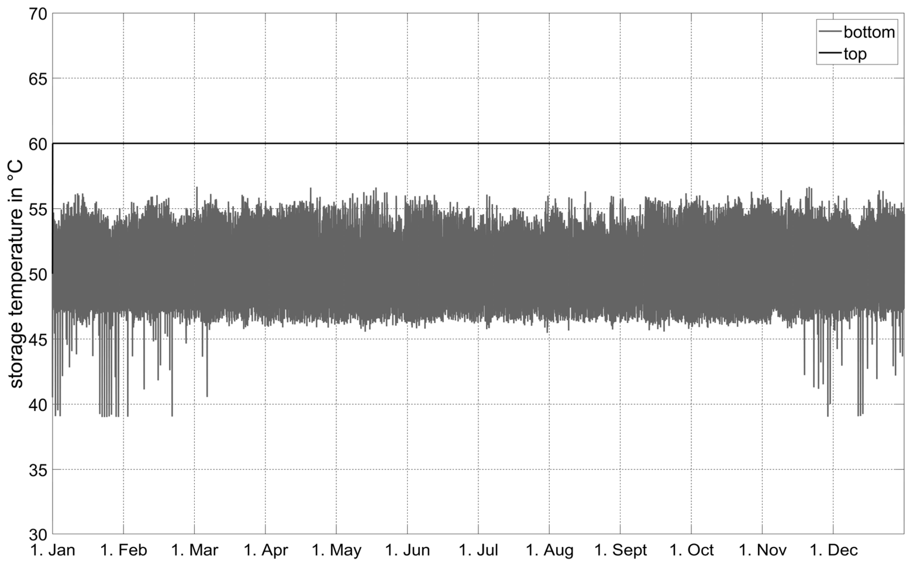
In the simulation without PV optimization, the heat pump is controlled in a way that the thermal storage can always provide the required supply temperature greater than 55 °C using the learned policy. This can be observed in Figure 9, showing a top storage temperature of a constant 60 °C.
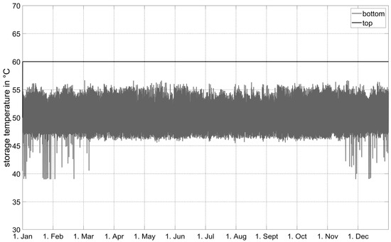
Figure 9.
Thermal storage temperatures from annual simulation without PV optimization.
Although the training included only six defined days of the year, one of which was randomly selected for each episode, the backup controller does not have to intervene on any day of the simulated year. Thus, the backup controller was only needed for proper training of the RL agent’s policy. Based on this result, the objective was extended to the PV-optimized heat pump operation.
Despite successful training using the TRPO agent for PV optimization, the self-consumption rate of 47.6% and the self-sufficiency of 16.6% are worse than for the basic controller. However, the simulation of the SAC agent shows an annual averaged improvement of almost 5% for both (see Table 6), which is less than the rule-based PV-optimized controller could achieve.

Table 6.
Simulation results of RL-based heat pump control strategies.
However, looking at the monthly self-consumption rates in Figure 5, in the winter months of November to January, the self-consumption rates are slightly higher than in the two reference cases with a maximum of 85.0% in January. They are lower for the rest of the year.
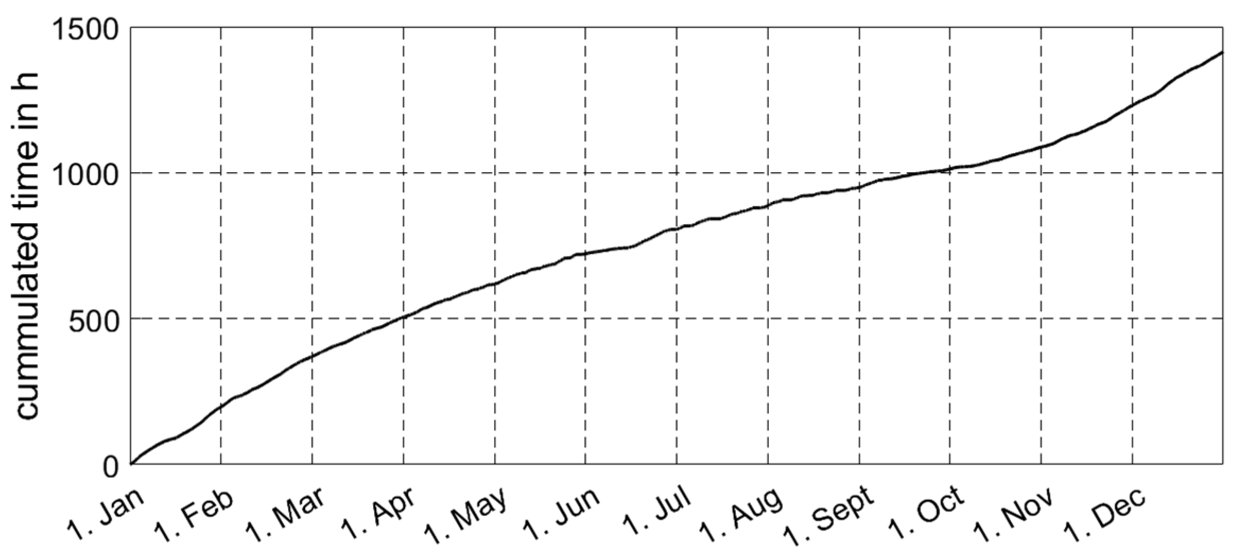
Further analysis showed that the backup controller intervened a total of 1415 h per year. As shown in Figure 10, intervention happened more often (bigger gradient) in winter to switch on the heat pump when the top storage temperature became too low than in summer (smaller gradient) to switch the heat pump off when the bottom storage temperature became too high.
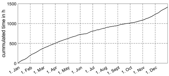
Figure 10.
Cumulated time of intervention of backup controller.
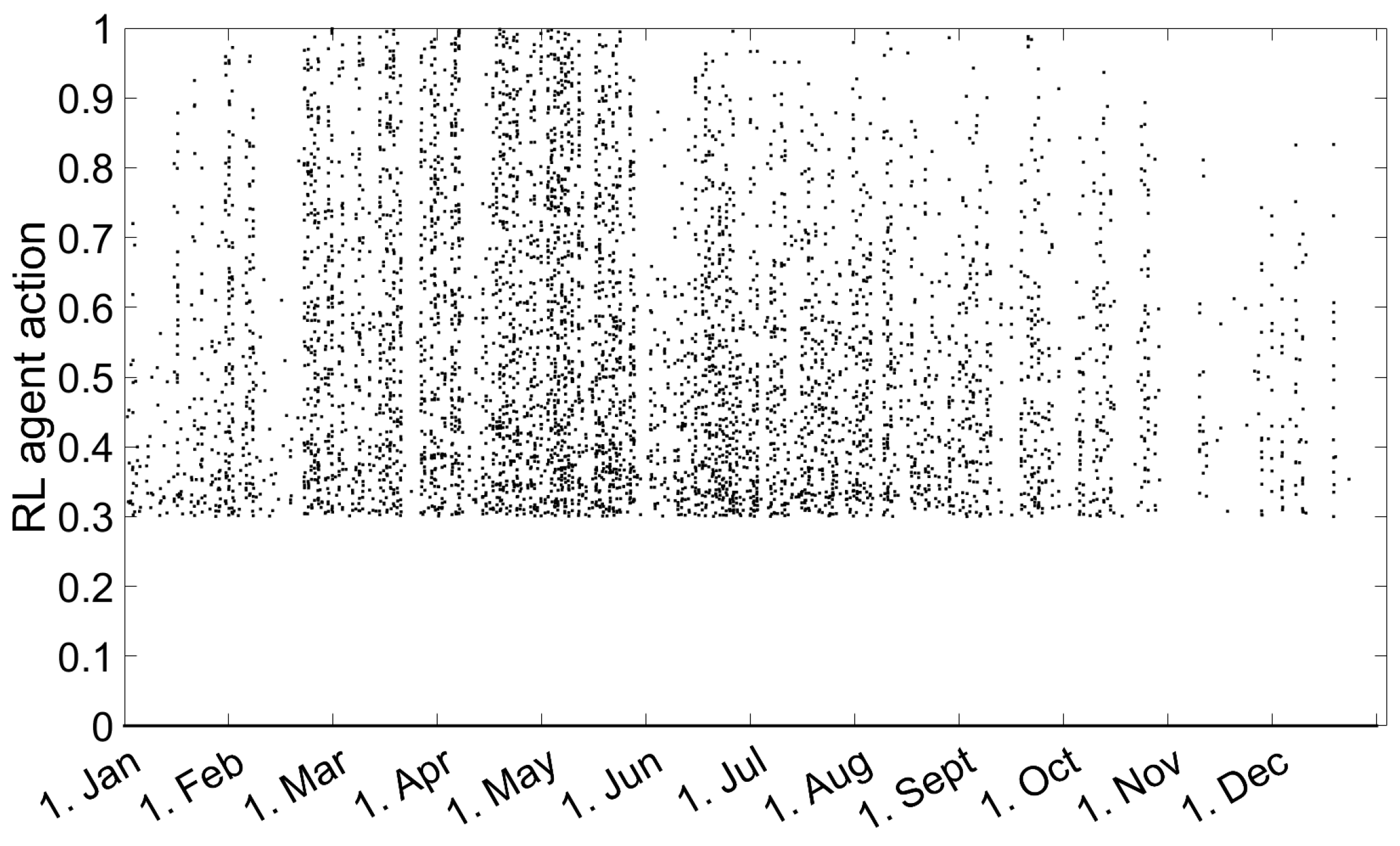
Looking at the actions chosen by the RL agent shown in Figure 11, there are too few actions in winter to switch on the heat pump, so the backup controller has to intervene.

Figure 11.
Actions chosen by PV-optimized SAC RL agent.
Finding an optimal way to teach the RL agent to handle two sometimes conflicting objectives in parallel seems to be difficult because, when there is no PV surplus, the actions should be low to avoid electricity consumption from the grid, but at the same time (mostly during the heating period), some action may be required to keep the storage temperatures in the required range. Thus, regarding the reward function (Equations (4)–(7)), it is difficult to define a trade-off in the weighting of the rewards for the storage temperatures and the electricity consumption from the grid. Another reason may be that training on only six randomly selected days of the year does not cover all situations that the agent needs to learn for a good policy.
Finally, it has to be mentioned that the developed RL-based controllers and the shown results only consider the weather of the location of Ingolstadt and a specific building type and dimension of the building energy system (e.g., heat pump and thermal storage). For the use of these controllers in other locations and for buildings with different load and generation profiles, a further training of the RL agent considering these different parameters is necessary.
4. Conclusions and Outlook
The detailed literature review conducted in this paper revealed a lack of investigation of RL-based controllers for multi-family building energy systems, including an air source heat pump, thermal storage, and a PV system. This gap is filled by this paper, which presents a novel investigation of RL-based controllers using a physical model that takes into account mass flows and temperatures in hydraulic circuits and thermal storages in detail. The model introduced for the development and simulation of RL-based controllers requires a variable time-step solver due to the complexity of the model. This is also a novelty compared to the related work using simplified models with constant time steps.
To evaluate the performance of RL-based controllers in this context, two rule-based controllers were defined and simulated for reference. One considers only the required temperatures in the thermal storage, and the other also optimizes the operation of the heat pump by shifting it to times of PV surplus to increase the self-consumption and self-sufficiency.
Four RL algorithms were investigated for each of the two RL-based controllers with the same two objectives as the reference controllers. For a successful training of the RL agents, a backup controller had to be implemented in the model to ensure the required storage temperatures. This also made it possible for the agent to explore bad choices resulting in negative rewards. Finally, the soft actor–critic method was selected for the annual simulations due to the highest rewards and a convergent training. It was shown that training a policy on only six defined days of the year results in an RL agent that successfully controls the heat pump to maintain the required storage temperatures for an entire year without intervention of the backup controller. The annual simulations of the RL-based PV optimization of the heat pump operation could only achieve a lower self-consumption rate of 50.3% and self-sufficiency of 17.6% than the rule-based PV-optimized controller (55.2%, 19.2%), while the backup controller had to intervene for 1.415 h per year. Thus, the trade-off between keeping the storage temperatures in the required range and shifting the heat pump operation to times of PV surplus seems to be challenging.
Due to the seasonality of the PV electricity generation (maximum in summer), which is opposite to the seasonality of the heat energy demand of the building (maximum in winter), it is suggested to extend the episode length for training to at least several days or a few weeks per season (winter, transition time, and summer) to cover longer time periods with larger variations in the ratios between heat load and PV electricity generation than only six days have. For this purpose, long short-term memory (LSTM) layers should be implemented in the policy to learn decisions that are based on both short-term and long-term experience. Future work to optimize this RL agent should also include a redesign of the reward function and further investigation of the hyperparameters.
Guidelines or suggestions for the correct choice of hyperparameter values for the different RL algorithms and their application to specific problems to be solved are missing in the literature. It would be very beneficial for future developments and a wider application of (D)RL approaches to collect and analyze hyperparameter settings in order to provide guidelines for developers.
Author Contributions
Conceptualization, M.B.; Methodology, M.B. and M.S.; Investigation, M.B. and M.S.; Writing—Original Draft, M.B.; Writing—Review and Editing, M.B., D.S., T.S. and C.T.; Supervision, W.Z.; Funding Acquisition, C.T. and W.Z. All authors have read and agreed to the published version of the manuscript.
Funding
This research was funded by Bayerische Forschungsstiftung, grant number AZ-1473-20. The APC was funded by Bayerische Forschungsstiftung and Technische Hochschule Ingolstadt. We acknowledge support by the Open Access Publication Fund of Technische Hochschule Ingolstadt (THI).
Data Availability Statement
Data are contained within the article.
Conflicts of Interest
The authors declare no conflicts of interest. The funders had no role in the design of the study; in the collection, analyses, or interpretation of data; in the writing of the manuscript; or in the decision to publish the results.
Nomenclature
| a | action value |
| Tbottom | bottom storage temperature |
| Tsup | supply water temperature |
| Ttop | top storage temperature |
| PPV,surp | power of photovoltaic system surplus |
| Psum | sum of electric power exchanged with the electricity grid |
| Abbreviations | |
| AI | artificial intelligence |
| BEM | building energy management |
| BMS | building management system |
| DDPG | deep deterministic policy gradient |
| DHW | domestic hot water |
| DR | demand response |
| DRL | deep reinforcement learning |
| HMS | home management systems |
| HVAC | heating, ventilation, and air conditioning |
| MILP | mixed-integer linear programming |
| MINLP | mixed-integer nonlinear programming |
| PV | photovoltaic |
| RL | reinforcement learning |
| RSAC | recurrent soft actor critic |
| SAC | soft actor–critic |
| SBEM | smart building energy management |
| TES | thermal energy storage |
| TRY | test reference year |
References
- Prognos; Öko-Institut; Wuppertal Institut. Towards a Climate-Neutral Germany by 2045. How Germany Can Reach Its Climate Targets before 2050. Executive Summary Conducted for Stiftung Klimaneutralität, Agora Energiewende and Agora Verkehrswende. 2021. Available online: https://www.agora-energiewende.org/fileadmin/Projekte/2021/2021_04_KNDE45/A-EW_213_KNDE2045_Summary_EN_WEB.pdf (accessed on 12 April 2024).
- Bongs, C.; Wapler, J.; Dinkel, A.; Miara, M.; Auerswald, S.; Lämmle, M.; Hess, S.; Kropp, M.; Eberle, R.; Rodenbücher, B.; et al. LowEx-Konzepte Für Die Wärmeversorgung von Mehrfamilien-Bestandsgebäuden. 2023. Available online: http://www.lowex-bestand.de/wp-content/uploads/2023/03/Abschlussbericht_LiB.pdf (accessed on 7 February 2024).
- Zator, S.; Skomudek, W. Impact of DSM on Energy Management in a Single-Family House with a Heat Pump and Photovoltaic Installation. Energies 2020, 13, 5476. [Google Scholar] [CrossRef]
- Kuboth, S.; Heberle, F.; König-Haagen, A.; Brüggemann, D. Economic model predictive control of combined thermal and electric residential building energy systems. Appl. Energy 2019, 240, 372–385. [Google Scholar] [CrossRef]
- Langer, L.; Volling, T. A reinforcement learning approach to home energy management for modulating heat pumps and photovoltaic systems. Appl. Energy 2022, 327, 120020. [Google Scholar] [CrossRef]
- Dounis, A.I.; Caraiscos, C. Advanced control systems engineering for energy and comfort management in a building environment—A review. Ren. Sust. Energy Rev. 2009, 13, 1246–1261. [Google Scholar] [CrossRef]
- Alanne, K.; Sierla, S. An overview of machine learning applications for smart buildings. Sust. Cities Soc. 2022, 76, 103445. [Google Scholar] [CrossRef]
- Sutton, R.S.; Barto, A.G. Reinforcement Learning: An Introduction, 2nd ed.; MIT Press: Cambridge, UK, 2018; p. 2. ISBN 9780262039246. [Google Scholar]
- Vázquez-Canteli, J.R.; Nagy, Z. Reinforcement learning for demand response: A review of algorithms and modeling techniques. Appl. Energy 2019, 235, 1072–1089. [Google Scholar] [CrossRef]
- Yu, L.; Xie, W.; Xie, D.; Zou, Y.; Zhang, D.; Sun, Z.; Zhang, L.; Zhang, Y.; Jiang, T. Deep reinforcement learning for smart home energy management. IEEE Internet Things J. 2020, 7, 2751–2762. [Google Scholar] [CrossRef]
- Yu, L.; Qin, S.; Zhang, M.; Shen, C.; Jiang, T.; Guan, X. A review of deep reinforcement learning for smart building energy management. IEEE Internet Things J. 2021, 8, 12046–12063. [Google Scholar] [CrossRef]
- Shaquor, A.; Hagishima, A. Systematic Review on Deep Reinforcement Learning-Based Energy Management for Different Building Types. Energies 2022, 15, 8663. [Google Scholar] [CrossRef]
- Wu, D.; Rabusseau, G.; Francois-lavet, V.; Precup, D.; Boulet, B. Optimizing Home Energy Management and Electric Vehicle Charging with Reinforcement Learning. In Proceedings of the ALA 2018—Workshop at the Federated AI Meeting 2018, Stockholm, Denmark, 14 July 2018; Available online: http://ala2018.it.nuigalway.ie/papers/ALA_2018_paper_37.pdf (accessed on 14 March 2024).
- Wang, Z.; Hong, T. Reinforcement learning for building controls: The opportunities and challenges. Appl. Energy 2020, 269, 115036. [Google Scholar] [CrossRef]
- Fu, Q.; Han, Z.; Chen, J.; Lu, Y.; Wu, H.; Wang, Y. Applications of reinforcement learning for building energy efficiency control: A review. J. Build. Eng. 2022, 50, 104165. [Google Scholar] [CrossRef]
- Perera, A.T.D.; Kamalaruban, P. Applications of reinforcement learning in energy systems. Ren. Sust. Energy Rev. 2021, 137, 110618. [Google Scholar] [CrossRef]
- Mason, K.; Grijalva, S. A Review of Reinforcement Learning for Autonomous Building Energy Management. Comp. El. Eng. 2019, 78, 300–312. [Google Scholar] [CrossRef]
- Ye, Y.; Wu, X.; Strbac, G.; Ward, J. Model-Free Real-Time Autonomous Control for a Residential Multi-Energy System Using Deep Reinforcement Learning. IEEE Trans. Smart Grid 2020, 11, 3068–3082. [Google Scholar] [CrossRef]
- Zsembinszki, G.; Fernández, C.; Vérez, D.; Cabeza, L.F. Deep Learning Optimal Control for a Complex Hybrid Energy Storage System. Buildings 2021, 11, 194. [Google Scholar] [CrossRef]
- Glatt, R.; da Silva, F.L.; Soper, B.; Dawson, W.A.; Rusu, E.; Goldhahn, R.A. Collaborative energy demand response with decentralized actor and centralized critic. In Proceedings of the 8th ACM International Conference on Systems for Energy-Efficient Buildings, Cities, and Transportation, Coimbra, Portugal, 17–18 November 2021; ACM: New York, NY, USA, 2021; pp. 333–337. [Google Scholar]
- Kathirgamanathan, A.; Twardowski, K.; Mangina, E.; Finn, D.P. A Centralised soft actor critic deep reinforcement learning approach to district demand side management through CityLearn. In Proceedings of the 1st International Workshop on Reinforcement Learning for Energy Management in Buildings & Cities, Online, 17 November 2020; ACM: New York, NY, USA, 2020; pp. 11–14. [Google Scholar]
- Ludolfinger, U.; Zinsmeister, D.; Perić, V.; Hamacher, T.; Hauke, S.; Martens, M. Recurrent Soft Actor Critic Reinforcement Learning for Demand Response Problems. In Proceedings of the IEEE PowerTech, Belgrade, Serbia, 27 June 2023. [Google Scholar] [CrossRef]
- MathWorks MATLAB. Available online: https://de.mathworks.com/products/matlab.html (accessed on 26 January 2024).
- MathWorks Simulink. Available online: https://de.mathworks.com/products/simulink.html (accessed on 26 January 2024).
- CARNOT Toolbox. Available online: https://www.fh-aachen.de/forschung/institute/sij/carnot (accessed on 26 January 2024).
- MathWorks Reinforcement Learning Toolbox. Available online: https://de.mathworks.com/products/reinforcement-learning.html (accessed on 26 January 2024).
- Loga, T.; Stein, B.; Diefenbach, N.; Born, R. Deutsche Wohngebäudetypologie-Beispielhafte Maßnahmen zur Verbesserung der Energieeffizienz von Typischen Wohngebäuden; Institut Wohnen und Umwelt: Darmstadt, Germany, 2015; Available online: http://www.building-typology.eu/downloads/public/docs/brochure/DE_TABULA_TypologyBrochure_IWU.pdf (accessed on 7 February 2024).
- SIA 2024: Raumnutzungsdaten für die Energie-und Gebäudetechnik; Schweizerischer Ingenieur und Architektenverein SIA: Zürich, Switzerland, 2015.
- DWD Deutscher Wetterdienst. Testreferenzjahre. 2017. Available online: https://www.dwd.de/DE/leistungen/testreferenzjahre/testreferenzjahre.html (accessed on 7 February 2024).
- VDI 4655: Heizungsanlagen mit Wärmepumpen in Ein- und Mehrfamilienhäusern Planung, Errichtung, Betrieb; Verein Deutscher Ingenieure e.V. VDI: Düsseldorf, Germany, 2018.
- Bachseitz, M.; Sheryar, M.; Schmitt, D.; Summ, T.; Trinkl, C.; Zörner, W. Reinforcement Learning for Building Energy System Control in Multi-Family Buildings. In Proceedings of the Solar World Congress, New-Delhi, India, 3 November 2023. in press. [Google Scholar]
- The MathWorks, Inc. Reinforcement Learning ToolboxTM—User’s Guide; The MathWorks, Inc.: Natick, MA, USA, 2023. [Google Scholar]
- Milan, C.; Bojesen, C.; Nielsen, M.P. A cost optimization model for 100% renewable residential energy supply systems. Energy 2012, 48, 118–127. [Google Scholar] [CrossRef]
- Quaschning, V. Understanding Renewable Energy Systems, 2nd ed.; Earthscan/Routledge: London, UK, 2016; p. 233. ISBN 978-1-138-78194-8. [Google Scholar]
Disclaimer/Publisher’s Note: The statements, opinions and data contained in all publications are solely those of the individual author(s) and contributor(s) and not of MDPI and/or the editor(s). MDPI and/or the editor(s) disclaim responsibility for any injury to people or property resulting from any ideas, methods, instructions or products referred to in the content. |
© 2024 by the authors. Licensee MDPI, Basel, Switzerland. This article is an open access article distributed under the terms and conditions of the Creative Commons Attribution (CC BY) license (https://creativecommons.org/licenses/by/4.0/).

