Adjustable Robust Energy Operation Planning under Uncertain Renewable Energy Production

Abstract

In this paper, the application of the method of affinely adjustable robust optimization to a planning model of an energy system under uncertain parameters is presented, and the total scheduling costs in comparison with the deterministic model are evaluated. First, the basics of optimization under uncertain data are recapped, and it is described how these methods can be used in different applications for energy systems. This is followed by the methodology of adjustable robust optimization by defining the affinely adjustable robust counterpart. Finally, a numerical case study is conducted to compare the adjustable robust method with a rolling deterministic scheduling method. Both are implemented on a model of an energy system and compared with each other by simulation using real-world data. By calculating the total operating costs for both methods, it can be concluded that the adjustable robust optimization provides a significantly more cost-effective solution to the scheduling problem.

1. Introduction

The expansion of renewable energy production is an important step to reduce CO₂ emissions and, thus, to slow down global warming. However, with a higher amount of weather-dependent energy sources like solar and wind power production and with uncertainty attached to the respective forecasts, it is more challenging to ensure a safe power supply.

The operation of an energy system involves scheduling several components, including devices to generate, store, and transform different types of energy, e.g., electrical and thermal, and the purchase and sale of energy. Typically, the amount of power that each of these components provides in a given time interval has to be determined in advance, and a time-dependent and cost-optimized schedule for the purchase and sale of electrical energy must be set; see, e.g., [1]. Now, if parts of the data in this optimization problem are uncertain or unknown in advance, e.g., the power output of a photovoltaic module, the decision maker has to use some nominal data, i.e., a forecast series, instead. In this case, deterministic optimization based on nominal values is the state of the art. This method is used to find the optimal sizing and configuration of hybrid power systems in [2,3,4]. Deterministic optimization as a suitable method for the short-term planning of energy systems is described in [5,6] and in combination with a rolling horizon strategy in [7,8,9]. Furthermore, in [10], a deterministic peak shaving strategy is studied, and in [11], an energy optimization scheduling strategy for an integrated energy system based on multi-time-scale coordination is proposed. When the deviation of the realized data from the nominal one is too high, it can happen that the inherent flexibility of the energy system is not sufficient to keep the previously calculated schedule. For example, if power production does not meet demand, the energy system operator is forced to spontaneously purchase the so-called imbalance energy from the grid, which usually entails enormous additional costs [12].

In contrast with this deterministic way of dealing with uncertain data, the methods of robust and stochastic optimization provide an optimal solution that takes other possible outcomes of the uncertainties into account and therefore avoid or lower the probability of these high imbalance compensation costs. In [13], a brief review of optimization methods under uncertainties for energy systems is given. Robust optimal planning is based on the worst possible realization regarding the cost function, while stochastic programming yields the optimal solution for the expected value of all scenarios. The advantage of robust optimization in comparison with the deterministic and stochastic methods is that the solution is feasible for all deviations from the nominal data. This is sometimes too conservative since the worst-case scenario is rarely realized and therefore related to unnecessarily high planning costs. Robust optimization and its variants are often applied to risk-averse scenarios. In energy economics, this could be island microgrids, since any imbalance between demand and supply can only be compensated by using storage facilities with limited capacity and power. To learn more about the application of robust optimization in island microgrids, see [14]. The advantages and disadvantages of robust planning in energy system optimization under uncertainties are discussed in several papers; see [15,16,17,18,19]. For less risk-averse use cases, stochastic optimization can be a better choice because only highly probable and less expensive scenarios are taken into account [20]. For applications of stochastic optimization in energy economics, the authors in [19] describe in which cases it is suitable and how to implement it in the program instead of the robust method.

In this paper, an extension of the robust optimization method, the so-called adjustable robust optimization, is briefly recapped, applied, and then evaluated. The underlying idea of this method is to include the possibility of adapting specific parts of the solution after some of the uncertain data have already become known in the planning phase. Now, it is to distinguish between here-and-now and wait-and-see variables. The former have to be determined in advance and therefore need to be robust against unknown deviations from the nominal data, while the latter are dependent on the uncertain data and can be adjusted accordingly after some or all of the realizations happen. Using this additional information, a less conservative solution can be found, resulting in significant savings in planning costs. Since the solution of an energy operation planning problem is a time-dependent schedule and some of the decisions can be made during the process, the method of adjustable robust optimization is well suited for this application. In [21], the idea of using adjustable robust optimization to determine the provision of control reserve to a power system is discussed, and in [22], the authors investigate an adjustable robust approach for dispatching island microgrids.

The case study presented in this paper, however, shows an application for the day-ahead planning of the cross-sectoral energy system of a living quarter based on real-world data with the aim of ensuring a control policy for all possible disturbance realizations under minimal balancing energy usage.

In Section 2, the basics of optimization under uncertain data are introduced, and it is described how these methods are used in different applications for energy systems. This is followed by the methodology of affinely adjustable robust optimization (AARO) in Section 3. Finally, a numerical case study is carried out to compare the AARO method with a rolling deterministic scheduling method. Both are implemented on a model representing the cross-sectoral energy system of a residential quarter and compared with each other by simulating historical realizations.

2. State of the Art

2.1. Deterministic Optimization

The common way of optimizing without any uncertain parameter is deterministic optimization. Linear or mixed integer linear formulations are often chosen for problems with a high number of variables, such as those used in the scheduling of energy systems. This has the advantage that high-performance solvers exist for this problem class, which are guaranteed to find globally optimal solutions in a short time. Deterministic scheduling models can be formulated as a linear program:

$$\underset{x\in {\mathbb{R}}^n}{min}{c}^{\top }x+d,\mathrm{s}.\mathrm{t}.Ax\le b.$$

(1)

Here, $x\in {\mathbb{R}}^n$ is the vector of decision variables, $c\in {\mathbb{R}}^n$ and $d\in \mathbb{R}$ are the parameters of the objective function, and $A\in {\mathbb{R}}^{m\times n}$ forms together with $b\in {\mathbb{R}}^m$ the constraints. The parameters A, b, c, and d are the data of the optimization problem. In reality, most of the input data can never be determined exactly, and users of the method have to deal with this problem in another way.

2.2. Stochastic Optimization

One approach to model uncertainty in the data $(c,d,A,b)$ is in terms of random variables, while the optimization is performed with respect to the expectation value or other risk measures for uncertainty; see, e.g., [23]. To this end, knowledge of the distribution of the uncertain data is required. We follow the idea in [24] of a two-stage stochastic linear program with a decision variable x divided into $x=(z,y)$, where z are the decisions to be taken under incomplete information on the random variables and y are corrective actions after the full information is unveiled. Then, the respective two-stage stochastic linear program with fixed recourse is formulated as follows:

$$\begin{array}{cc}\hfill \underset{z\in {\mathbb{R}}^n}{min}{c}_0^{\top }z+d_0+{\mathbb{E}}_{\xi }\left[Q(z,\xi )\right],\mathrm{s}.\mathrm{t}.A_{0}z& \le b_0\hfill \end{array}$$

(2)

with $c_0\in {\mathbb{R}}^n$, $d_0\in \mathbb{R}$, $A_0\in {\mathbb{R}}^{m\times n}$, and $b_0\in {\mathbb{R}}^m$ being known data of the first-stage problem, while the stochastic variable $\xi$ models uncertainties. Provided an outcome $\omega$, the quantity $Q(x,\xi (\omega \left)\right)$ is given as the optimal value of the second-stage problem:

$$\begin{array}{c}\hfill \underset{y\in {\mathbb{R}}^r}{min}{c}_1{\left(\omega \right)}^{\top }y+d_1\left(\omega \right),\mathrm{s}.\mathrm{t}.A_1\left(\omega \right)z+A_{2}y\le b_1\left(\omega \right)\end{array}$$

(3)

with a fixed recourse matrix $A_2\in {\mathbb{R}}^{p\times r}$, and $\xi =(c_1,d_1,A_1,b_1)$, where $c_1\left(\omega \right)\in {\mathbb{R}}^r$, $d_1\left(\omega \right)\in \mathbb{R}$, $A_2\left(\omega \right)\in {\mathbb{R}}^{p\times n}$, and $b_1\left(\omega \right)\in {\mathbb{R}}^p$. The approach is now to first calculate the expectation value ${\mathbb{E}}_{\xi }\left[Q(x,\xi \left(\omega \right))\right]$ with respect to the random variable $\xi$ and obtain the so-called deterministic equivalent problem. Subsequently, the solution $z\in {\mathbb{R}}^n$ of the first-stage problem (2) can be determined, and after the realization of the outcome $\omega$, the second-stage problem (3) can be solved for the variable $y\in {\mathbb{R}}^r$.

For applications of stochastic optimization in energy economics, the authors in [19] describe in which cases it is suitable and how to implement it in the program instead of alternative approaches based on robust optimization as outlined in the following.

2.3. Robust Optimization

The method of robust optimization ensures the feasibility of the solution for all possible realizations and is formulated by the worst-case method, which will now be introduced as it is done by Ben-Tal et al. in [25] (p. 7). To model the uncertainties, a data matrix $D\in {\mathbb{R}}^{(m+1)\times (n+1)}$, with the following:

$$D=\left[\begin{array}{cc}{c}^{\top }& d\\ A& b\end{array}\right]$$

is introduced, where we identify the tuple $(c,d,A,b)$ with D. Let $D_0$ be the matrix of known reference data and $D_j$, $j\in \{1,\dots ,l\}$ be potential maximal deviations from the nominal values, which have to be known. The unknown parameter is now which entry deviates to what extent. This can be described using the uncertain perturbation vector $\zeta \in \mathcal{Z}$. Assuming the perturbation set $\mathcal{Z}$ to be a parallelotope, which is the image of a unit box under affine mapping, it can be normalized without loss of generality as follows:

$$\mathcal{Z}=\prod _{j=1}^l[-1,1]\subset {\mathbb{R}}^l.$$

(4)

Therefore, $\mathcal{Z}$ is the set of all possible perturbations, and l is the number of entries that deviate independently. The set of all uncertain data matrices:

$$\mathcal{U}=\left\{D=D_0+\sum _{j=1}^l{\zeta }_j{D}_j|\zeta \in \mathcal{Z}\right\}\subset {\mathbb{R}}^{(m+1)\times (n+1)},$$

called uncertainty set, gives rise to a family of linear programs of the form (1), which are parameterized via $(c,d,A,b)=D\in \mathcal{U}$. Such a family is referred to as uncertain linear optimization problem [25].

Uncertainties in the data c and d only affect the objective value, while uncertainty in A and b has an impact on the feasibility of the optimization problem. Therefore, it makes sense to define the concepts of robust feasibility and robust optimal value. The following set:

$$\mathcal{X}=\{x\in {\mathbb{R}}^n|Ax\le b\forall (c,d,A,b)\in \mathcal{U}\}$$

contains all robustly feasible solutions. For each robustly feasible solution $\widehat{x}\in \mathcal{X}$, the robust value is the largest value of the objective $c^{\top }\widehat{x}+d$ that is attained over $\mathcal{U}$, i.e.,

$$\underset{(c,d,A,b)\in \mathcal{U}}{sup}{c}^{\top }\widehat{x}+d.$$

This definition corresponds to the idea of the worst-case method. It is to minimize the robust value over all robustly feasible solutions, which leads to the following definition of the robust counterpart (RC) of the uncertain linear problem:

$$\begin{array}{c}\hfill \underset{x\in {\mathbb{R}}^n}{min}\underset{(c,d,A,b)\in \mathcal{U}}{sup}{c}^{\top }x+d\\ \hfill \mathrm{s}.\mathrm{t}.Ax\le b\\ \hfill \forall (c,d,A,b)\in \mathcal{U}.\end{array}$$

(5)

One can show that the RC (5) can be represented as a linear program with the constraint parameter A being the only uncertainty, while the right-hand side b and the parameters c and d in the objective function are deterministic, cf. [26]. Further, it can be assumed without loss of generality that the left-hand side of the constraints is affine functions in the uncertainty $\zeta$, and also the uncertainty set can be formulated constraint-wise; see [26]. Under these assumptions, the semi-infinite robust counterpart can be solved and reformulated as a computationally tractable linear program with a finite number of constraints. This worst-case formulation is exemplarily carried out in [26] in a single constraint.

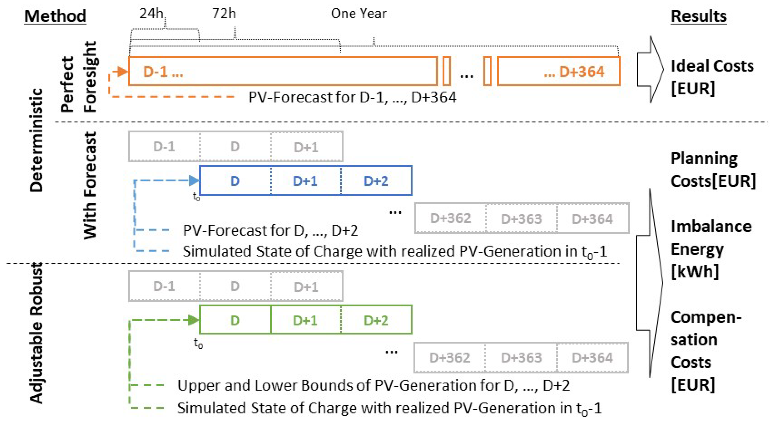
3. Adjustable Robust Optimization

Consider the following robust optimization problem:

$$\begin{array}{c}\hfill \underset{x\in {\mathbb{R}}^n,s\in \mathbb{R}}{min}s\\ \hfill \mathrm{s}.\mathrm{t}.c^{\top }x& \le s\hfill \\ \hfill A\left(\zeta \right)x& \le b\forall \zeta \in \mathcal{Z},\hfill \end{array}$$

with deterministic c and b, which is equivalent to the RC (5) after a suitable relabeling [26]. As before, the uncertainty is modeled as affinely linear, i.e., $A\left(\zeta \right)=A_0+{\sum }_{j=1}^l{\zeta }_j{A}_j$, over the perturbation set $\mathcal{Z}\subset {\mathbb{R}}^l$ given as in (4). The idea of adjustable robust optimization is to divide the variables $x_j$ into here-and-now and wait-and-see decisions and to substitute the latter with functions, the so-called decision rules, $y_j\left(P_j\zeta \right)$, which are dependent on $\zeta$. The diagonal matrix $P_j\in {\{0,1\}}^{l\times l}$ represents the information base and determines for each variable $x_j$ which entries of $\zeta$ are already known. The resulting adjustable robust counterpart (ARC) is formulated as follows:

$$\begin{array}{c}\hfill \underset{s\in \mathbb{R},y\left(·\right)}{min}s\\ \hfill \mathrm{s}.\mathrm{t}.c^{\top }y\left(\zeta \right)& \le s\hfill \\ \hfill A\left(\zeta \right)y\left(\zeta \right)& \le b\forall \zeta \in \mathcal{Z},\hfill \end{array}$$

where $y\left(\zeta \right)=(y_1\left(P_1\zeta \right),\dots ,y_n\left(P_n\zeta \right))$ are the decision rules. The solutions’ dependency on the uncertainty parameter allows the ARC more flexibility than the RC. Consequently, the ARC leads to a larger robust feasible set, which may result in an improved optimal value. The decision rules are often approximated with affine functions since, otherwise, the program is generally not computationally tractable. Using affine decision rules $y_j\left(P_j\zeta \right)=p_j+q_j^{\top }{P}_j\zeta$ with $p_j\in \mathbb{R}$ and $q_j\in {\mathbb{R}}^l$, $j\in \{1,\dots ,n\}$, the affinely adjustable robust counterpart (AARC) can be defined as follows:

$$\begin{array}{c}\hfill \underset{s,{\{p_j,q_j\}}_{j=1}^n}{min}s\\ \hfill \mathrm{s}.\mathrm{t}.\sum _{j=1}^n{c}_j(p_j+q_j^{\top }{P}_j\zeta )& \le s\hfill \\ \hfill \sum _{j=1}^n{a}_{ij}\left(\zeta \right)(p_j+q_j^{\top }{P}_j\zeta )& \le b_i,\forall i\in \{1,\dots ,m\},\forall \zeta \in \mathcal{Z}.\hfill \end{array}$$

The optimization variables of this problem are now $t\in \mathbb{R}$ and the coefficients $p_j$ and $q_j$ of the decision rules. In the case of fixed recourse, i.e., when the coefficients $a_{ij}$ are constant in ${\zeta }_j$ for $P_j\ne 0$, AARC is as tractable as the RC of the problem. Otherwise, these coefficients are quadratic in $\zeta$, and the tractability of AARC cannot be guaranteed. For the case study in this paper, affinely adjustable robust optimization will be applied.

Ben-Tal et al. prove in [25] (p. 368) that the ARC and RC of an uncertain linear problem are equivalent with the same optimal value if the uncertainty is constraint-wise, which means that the ARC only can yield better results than the RC if this assumption does not hold; i.e., the vector $\zeta$ cannot be split into blocks ${\zeta }_0,\dots ,{\zeta }_m$ such that the i-th constraint depends solely on ${\zeta }_i$. This result is essential for appropriate modeling in order to obtain better optimal values using the adjustable robust method. On the other hand, it means that if the uncertainties are not constraint-wise, the above-mentioned worst-case formulation cannot be applied to reformulate the semi-infinite ARC as a computationally tractable program. In this case, if the uncertainty set is computationally tractable, e.g., box uncertainty, it is indeed possible to represent each semi-infinite constraint by a system of linear inequalities, which is proven in [25] (p. 20). AARC problems are closely related to affinely adjustable robust complementary problems, which are investigated in [27] regarding the existence and uniqueness of robust solutions. Moreover, these kinds of problems allow for a mixed-integer programming formulation that can be used to compute solutions [27,28].

4. Numerical Case Study

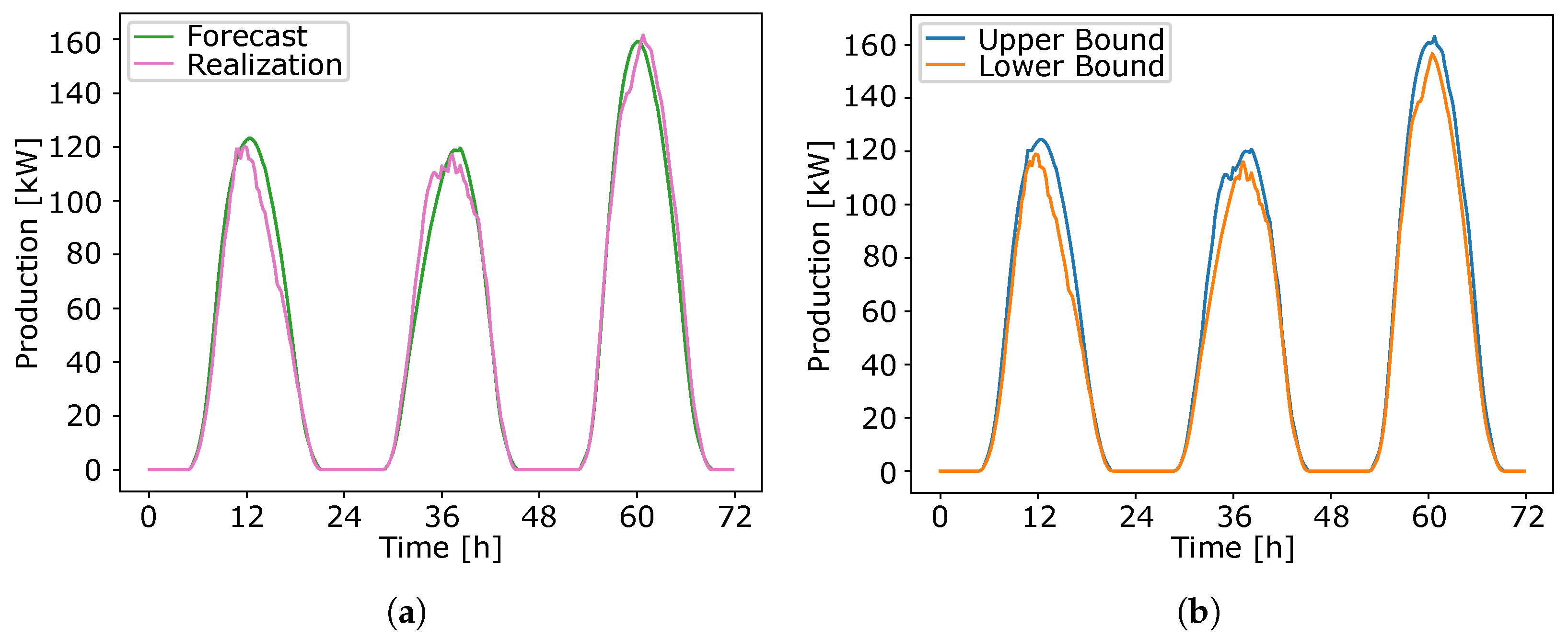
4.1. Use Case

The subject of this case study is a cross-sectoral energy system that is part of the research project “ODH@Bochum-Weitmar” of Open District Hub e.V. for the development of sustainable concepts of energy supply for an existing living quarter in Bochum-Weitmar, Germany; see [29,30] and Figure 1. The parameters for the components, which are solar power production, a battery, hydrogen and heat storage, heat pumps, a fuel cell, a gas boiler, household load characteristics, and the power grid, are slightly modified values from [30]. The electricity load is generated using the load profile generator [31] for an average household in Germany, and the heat load is based on a building simulation in the context of the project “ODH@Bochum-Weitmar”; see also [32,33,34]. The purchase prices for electricity and gas are assumed to be realistic values at the beginning of the project, and the feed-in compensation comes from the “Bundesnetzagentur” [35]. The considered uncertainty in this energy system is the generation of the photovoltaic plant. The predicted and realized photovoltaic infeed time series are taken from [35] for the control area 50Hertz in Germany in the year 2021 and scaled to a maximal power of $183,4$ $\mathrm{k}$$\mathrm{W}$, which corresponds to a module with a nominal power of 200 $\mathrm{kWp}$.

4.2. Deterministic Model

In order to compute the most cost-efficient schedule for the energy system, a deterministic linear optimization model with a time period of 1 year and a granularity of 15 min is first introduced. The objective is to minimize the total purchase costs for electricity and gas and to maximize the feed-in compensation for the electricity surplus over the entire time horizon, where the decision variables represent the power of each component in kilowatts per 15 min. The constraints of the optimization problem include balance equations for electricity, heat, hydrogen, and gas. Additionally, there are restrictions on the components, like capacity, nominal power, efficiency, coefficient of performance, and limits for purchasing and delivering power. The decision variable of the linear program consists of the components listed in

Table 1. Variables of the deterministic problem.

Component	Symbol [Unit]
Power purchase	$p_{el}$ [kW]
Gas purchase	$p_{gas}$ [kW]
Power delivery	$d_{el}$ [kW]
Battery storage SOC 1/input/output	$B_{SOC}$ [kWh]/$B_{in}/B_{out}$ [kW]
$H_2$-storage SOC/input/output	$H_{SOC}$ [kWh]/$H_{in}/H_{out}$ [kW]
Heat buffer SOC/input/output	$Q_{SOC}$ [kWh]/$Q_{in}/Q_{out}$ [kW]
CHP 2 electric and thermal power input/output	$CH{P}_{el,in}/CH{P}_{el,out}$, $CH{P}_{th,in}/CH{P}_{th,out}$ [kW]
Gas boiler input/output	$G_{in}/G_{out}$ [kW]
Electrolyzer input/output	$El{y}_{in}/El{y}_{out}$ [kW]
Air-source heat pump input/output	$ASH{P}_{in}/ASH{P}_{out}$ [kW]
Ground-source heat pump input/output	$GSH{P}_{in}/GSH{P}_{out}$ [kW]

¹ SOC: state of charge. ² CHP: combined heat and power (cogeneration) plant.

and is given by the following:

$$\begin{array}{c}\hfill x={\left(p_{el}\left(t\right),p_{gas}\left(t\right),d_{el}\left(t\right),B_{SOC}\left(t\right),B_{in}\left(t\right),B_{out}\left(t\right)\cdots ,GSH{P}_{in}\left(t\right),GSH{P}_{out}\left(t\right)\right)}_{t=1}^T,\end{array}$$

where t represents a discrete time instance and T is the considered horizon. The parameters of the linear program are shown in

Table 2. Parameters of the deterministic problem.

Component	Symbol [Unit]	Value
PV production	$pv$ [kW]	time series
Electricity load	$loa{d}_{el}$ [kW]	time series
Heat load	$loa{d}_Q$ [kW]	time series
Electricity buy price	$k_{el}$ [Euro/kWh]	0.34281
Max electricity purchase	$p_{el.max}$ [kW]	1000
Gas price	$k_{gas}$ [Euro/kWh]	0.066965
Max gas purchase	$e_{gas.max}$ [kW]	1000
Electricity sell price	$k_d$ [Euro/kWh]	0.07
Max electricity delivery	$d_{max}$ [kW]	1000
Nominal power gas boiler	$P_G$ [kW]	800
Efficiency gas boiler	${\eta }_G$ [%]	90
Capacity battery storage	$C_B$ [kWh]	250
Nominal power battery storage	$P_B$ [kW]	55
Efficiency	${\eta }_B$ [%]	97.9
Capacity $H_2$-storage	$C_H$ [kWh]	2.7
Nominal power $H_2$-storage	$P_H$ [kW]	1
Efficiency	${\eta }_H$ [%]	100
Capacity heat buffer	$C_Q$ [kWh]	20
Nominal power heat buffer	$P_Q$ [kW]	5
Efficiency heat buffer	${\eta }_Q$ [%]	95
Electric power CHP	$P_{CHP.el}$ [kW]	24.7
Electrical efficiency CHP	${\eta }_{CHP.el}$ [%]	26.1
Thermal power CHP	$P_{CHP.th}$ [kW]	36
Thermal efficiency CHP	${\eta }_{CHP.th}$ [%]	38.1
Nominal power electrolyzer	$P_{Ely}$ [kW]	9.6
Efficiency electrolyzer	${\eta }_{Ely}$ [%]	73.5
Nominal power air-source heat pump	$P_{ASHP}$ [kW]	2.5
COP 1 air-source heat pump	${\eta }_{ASHP}$	4
Nominal power ground-source heat pump	$P_{GSHP}$ [kW]	12.8
COP ground-source heat pump	${\eta }_{GSHP}$	4.38

¹ COP: coefficient of performance.

.

In order to minimize the loss from purchasing electrical power and gas over time $\{1,\cdots ,T\}$, while maximizing the revenue from delivering power, we consider the deterministic linear program:

$$\underset{x}{min}\frac{1}{4}\sum _{t=1}^T(k_{el}·p_{el}\left(t\right)+k_{gas}·p_{gas}\left(t\right)-k_d·d_{el}\left(t\right))$$

with constraints formulated below. The factor $1/4$ serves as normalization in order to preserve units. One part of the constraints is covered by the balance equations for electricity:

$$\begin{array}{c}\hfill \begin{array}{cc}\hfill pv\left(t\right)+p_{el}\left(t\right)+B_{out}\left(t\right)+CH{P}_{el,out}\left(t\right)=d_{el}\left(t\right)+loa{d}_{el}\left(t\right)& + El{y}_{in}\left(t\right)+ASH{P}_{in}\left(t\right)\hfill \\ \hfill & + GSH{P}_{in}\left(t\right)+B_{in}\left(t\right)\hfill \end{array}\end{array}$$

(6)

and for heat:

$$G_{out}\left(t\right)+ASH{P}_{out}\left(t\right)+GSH{P}_{,out}\left(t\right)+CH{P}_{th,out}\left(t\right)+Q_{out}\left(t\right)=Q_{in}\left(t\right)+loa{d}_Q\left(t\right)$$

(7)

for all $t\in \{1,\cdots ,T\}$. All components that produce or output power are on the left, and consumers or components that input power are on the right-hand side of Equations (6) and (7). The $H_2$-flow from the electrolyzer through a $H_2$-storage into a fuel cell, which then generates heat and electric power simultaneously (cogeneration), is described by the following:

$$\begin{array}{cc}\hfill El{y}_{out}\left(t\right)& =H_{in}\left(t\right),\hfill \\ \hfill H_{out}\left(t\right)& =CH{P}_{el,in}\left(t\right),\hfill \\ \hfill H_{out}\left(t\right)& =CH{P}_{th,in}\left(t\right),\forall t\in \{1,\cdots ,T\}.\hfill \end{array}$$

The gas flow from purchase into the gas boiler is implemented by the following balance equation:

$$p_{gas}\left(t\right)=G_{in}\left(t\right),\forall t\in \{1,\cdots ,T\}.$$

The state evolution for the storage units can be described by the following:

$$S_{SOC}\left(t\right)=\sum _{j=1}^t\frac{1}{4}\left(S_{in}\left(j\right)-\frac{100·S_{out}\left(j\right)}{{\eta }_S}\right),\forall t\in \{1,\cdots ,T\},\forall S\in \{B,H,Q\}.$$

In this particular situation, the initial charge at time $t=0$ is zero. Further, the state of charge is bounded by the capacity, and the power in- and output are bounded by the nominal power of the storage unit:

$$\begin{array}{cc}\hfill S_{SOC}\left(t\right)& \le C_S\hfill \\ \hfill S_{in}\left(t\right),S_{out}\left(t\right)& \le P_S,\forall t\in \{1,\cdots ,T\},\forall S\in \{B,H,Q\}.\hfill \end{array}$$

The efficiency constraints of the CHP, the gas boiler, the electrolyzer, and the COP of the heat pumps are modeled through the following:

$$u_{in}\left(t\right)=\frac{100·u_{out}\left(t\right)}{{\eta }_u},\forall t\in \{1,\cdots ,T\},\forall u\in \{CH{P}_{el},CH{P}_{th},G,Ely,ASHP,GSHP\}.$$

The output of all generation units u is bounded by their nominal power:

$$u_{out}\left(t\right)\le P_u,\forall t\in \{1,\cdots ,T\},u\in \{CH{P}_{el},CH{P}_{th},G,Ely,ASHP,GSHP\}.$$

Similarly, the electricity and gas purchase and the power delivery are limited:

$$\begin{array}{cc}\hfill p_{el}\left(t\right)& \le p_{el,max}\hfill \\ \hfill p_{gas}\left(t\right)& \le p_{gas,max}\hfill \\ \hfill d_{el}\left(t\right)& \le d_{max},\forall t\in \{1,\cdots ,T\}.\hfill \end{array}$$

(8)

Finally, we impose the non-negativity of the decision variables, i.e., $x\ge 0$.

The solution for this deterministic problem can be found using common solvers for linear programs. The uncertain parameter $pv$ is a forecast time series without any deviations.

4.3. Adjustable Robust Model

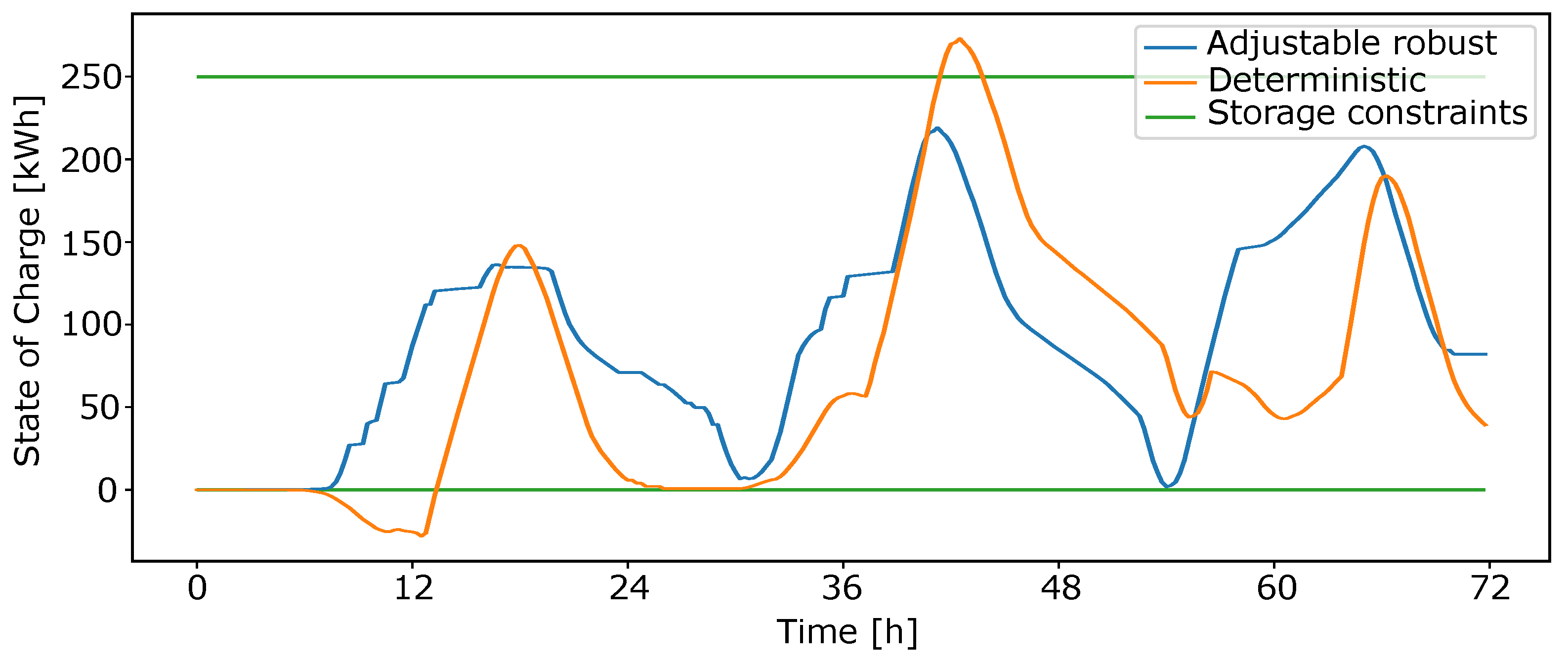
The application context of the affinely adjustable robust method (ARO) is to consider a time horizon of 72 h since the weather forecast for 3 days can be expected to be accurate enough. After every 24 h, which corresponds to 96 15-min time steps, the realized power production and, therefore, the real state of charge of the battery storage are known, and the decision maker is allowed to adjust the solution regarding the previously calculated power purchase and sale schedule based on these known parameters. Consequently, the information base $I_t$ is modeled as follows:

$$I_t=\left\{\begin{array}{cc}\varnothing \hfill & \mathrm{for}t\in \{1,\dots ,96\}\hfill \\ \{1,\dots ,96\}\hfill & \mathrm{for}t\in \{97,\dots ,192\}\hfill \\ \{1,\dots ,192\}\hfill & \mathrm{for}t\in \{193,\dots ,288\}.\hfill \end{array}\right.$$

In the mathematical context, the electricity purchase $p_{el}$ is chosen as the adjustable wait-and-see variable and substituted with the affine function:

$$p_{el}\left(t\right)=ϵ\left(t\right)+\sum _{k\in I_t}{E}_t\left(k\right)·pv\left(k\right),$$

(9)

where $ϵ$ and $E_t$ denote the new decision variables and $pv$ the once uncertain but, at time $t\in \{1,\cdots ,T\}$ for the information base $I_t$, known photovoltaic infeed. The uncertainty in solar power production is represented by a lower bound $\underline{pv}\left(t\right)$ and an upper bound $\overline{pv}\left(t\right)$ of the real data, which has been generated from the forecast and realization time series; see Figure 2a,b. It is ensured that the realization always lies in between those bounds and that the deviation is not too large, as otherwise, there does not exist a robust solution. The average deviation is 6.4% below and 3.9% above the forecast.

To pass from the deterministic to the robust formulation, it is necessary to eliminate balance equations containing uncertain parameters. In the case the balance equation for electricity (6), this is performed by substituting the power input of the battery in every constraint with the following:

$$\begin{array}{cc}\hfill B_{in}\left(t\right)=& pv\left(t\right)+(ϵ\left(t\right)+\sum _{k\in I_t}{E}_t\left(k\right)·pv\left(k\right))+B_{out}\left(t\right)+CH{P}_{el,out}\left(t\right)\hfill \\ \hfill & -\left(d_{el}\left(t\right)+loa{d}_{el}\left(t\right)+El{y}_{in}\left(t\right)+ASH{P}_{in}\left(t\right)+GSH{P}_{in}\left(t\right)\right)\hfill \end{array}$$

for all $t\in \{1,\cdots ,T\}$. This substitution also ensures that the uncertainty does not only appear constraint-wise; e.g., since the constraint of the battery state of charge is a state inequality, the i-th restriction contains, apart from $pv\left(i\right)$, also all previous $pv\left(1\right),\dots ,pv(i-1)$. Furthermore, since $\mathcal{Z}$ represents box uncertainty (see (4)), each semi-infinite constraint in the problem can be replaced by a system of linear inequalities, as demonstrated in [25] (p. 392). In this use case, it is carried out exemplarily for one simple constraint. By (8) and (9), the maximal value of purchased electricity $p_{el,max}$ is subject to the restriction:

$$\begin{array}{cc}\hfill ϵ\left(t\right)+\sum _{k\in I_t}{E}_t\left(k\right)·pv\left(k\right)& \le e_{el,max},\hfill \\ \hfill pv\left(t\right)& \le \overline{pv}\left(t\right),\hfill \\ \hfill pv\left(t\right)& \ge \underline{pv}\left(t\right)\hfill \end{array}$$

(10)

for all $t\in \{1,\dots ,T\}$. Introducing the additional variable $h_t\left(i\right)$ with $t,i\in \{1,\dots ,T\}$, the statement (10) is equivalent to the following:

$$\begin{array}{cc}\hfill & ϵ\left(t\right)+\sum _{k\in I_t}{h}_t\left(k\right)\le e_{el,max},\hfill \\ \hfill & E_t\left(k\right)·\underline{pv}\left(k\right)\le h_t\left(k\right),k\in I_t,\hfill \\ \hfill & E_t\left(k\right)·\overline{pv}\left(k\right)\le h_t\left(k\right),k\in I_t.\hfill \end{array}$$

This is carried out for all other constraints where the uncertain parameter $pv$ occurs to obtain a tractable robust counterpart, which can be solved by linear programming. In this study, the open-source solver CLP was used, which always terminated in reasonable time. In contrast with this, the deterministic rolling method is also allowed to compute a new here-and-now solution after 24 h according to the real state of charge but without considering any deviations from the forecast and also without the use of adjustable wait-and-see variables. An overview of the used methods, including the benchmark method of having the perfect foresight, is visualized in Figure 3. Here, D represents one 24 h time horizon, and $t_0$ is the beginning of every day, when the data about the realized PV-infeed of the previous day $t_0-1$ have become available. The outcome of the deterministic problem using the real PV production time series is the so-called ideal costs. These are used as a benchmark to compare and evaluate the results of the considered methods.

5. Results

For reasons of simplification, the results are demonstrated for one 72 h time period, i.e., 22–25 May 2021. The deterministic schedule is calculated using the predicted solar power input, while the adjustable robust model takes the generated upper and lower bounds. After simulating both solutions with the realized data, the total costs, consisting of the planning costs and the imbalance energy costs, are calculated. The realized state of charge of the battery storage is shown for both methods in Figure 4.

As can be seen, the deterministic solution violates the constraints on the state of charge, which is required to stay between zero and the storage capacity of 250 kWh. In case the energy system is short on energy, it has to purchase more energy as scheduled, and if it is long, it has to sell more. This imbalance energy has to be financially compensated by the operator of the energy system, which results in imbalance costs and also profits; see

Table 3. Comparison of both methods for 72 h time period.

Method	Deterministic	ARO
Planning costs	EUR 194.16	EUR 211.50
Imbalance energy	$453.27$ kWh shortage	0 kWh
	$140.40$ kWh surplus	0 kWh
Imbalance costs	EUR 155.39 loss	EUR 0
	EUR −9.83 profit	EUR 0
Total operational costs	EUR 339.72	EUR 211.50
Deviation from ideal costs	112.2%	32.1%
Performance	26 s	182 s

. In contrast, the adjustable solution is always able to keep the planned schedule for purchasing and selling electrical energy to the grid, so no imbalance energy is needed, and no extra costs are incurred. The imbalance energy price in this calculation is set to be the the same as the prices from the planning model, i.e., EUR 0.34281/kWh for purchase and EUR 0.07/kWh for feed-in compensation. The planning costs are the optimization value of the respective method, meaning the costs and revenue of the scheduled energy purchase and delivery. To obtain the total operational costs, the planning costs and the imbalance costs are added up. These results are shown in Table 3, also including the computation time and the deviation from the ideal costs. The ideal costs are used as a benchmark and are the optimal value for the deterministic problem using the realized photovoltaic generation instead of the forecast. In other words, this describes the operational costs if the real production data were known in advance, which means having the perfect foresight. For this use case, the calculation of the ideal costs yields EUR 160.06 with a computation time of 1.66 s.

Table 3 shows that the planning costs of the deterministic method are lower by 8.2% since it does not consider the worst case. However, when the imbalance costs are factored in, the adjustable robust solution outperforms the deterministic solution by 37.7%. In reality, even higher costs can be expected since the imbalance energy prices are usually much higher than the ones in the day-ahead auction. To compare the performances, the adjustable robust model computes six times longer than the deterministic one.

Now, this approach is taken for the entire time period from 1 January until 31 December 2021, and all costs are added up. It turns out that, in only three cases, a robust solution cannot be found due to too high deviations (up to 45%) of the uncertain data. The missing results are therefore replaced by the deterministic planning, and include the imbalance costs for the corresponding period. In total, the costs of the adjustable robust model are 26% lower than those of the deterministic model, but its performance is five times longer. The deviation from the ideal costs of the deterministic method is 45.2%, while that of the ARO is 7.4% for a time period of 1 year.

6. Discussion

The results of this case study show that the adjustable robust planning method is well suited to reduce operational costs for applications with uncertain parameters, especially time-dependent scenarios. In contrast with the deterministic method, it is protected against unpredictable parameter deviations and, additionally, is less conservative than static robust optimization due to a larger robust feasible set. That is because the adjustable robust optimization utilizes the known true values of the uncertain data that have been revealed by the respective information base, which also leads to an improved optimal value of the problem. Nevertheless, the adjustable robust method cannot yield a robust feasible solution for too large uncertainty sets. To resolve this issue, the uncertainty set may be adapted. On the one hand, the length of the optimization horizon may be reduced to reduce uncertainty. This would also be beneficial for robust optimization, but may deteriorate the overall performance. On the other hand, one may incorporate further dependencies to render the resulting robust optimization problem more adjustable, e.g., by providing either additional information or the same information earlier, which means updating the information basis more frequently. Both options would increase the number and/or the impact of the adjustable variables and, thus, reduce conservatism by shrinking the uncertainty set. In the considered case study, a reduction in the information delay from 24 to 12 h has a positive impact on feasibility. To conclude, the applier must assess the increased conservatism and longer computation time of the (affinely adjustable) robust method in comparison with potentially higher compensation costs due to eventually infeasible solutions resulting from deterministic optimization; see, e.g., [36] or [37] and the references therein for multiobjective optimization in general. According to the results presented in Section 5, the adjustable robust method outperforms the deterministic method already for relatively low balance energy prices such that the significantly improved performance easily justifies the up-to-six-times-longer computation time if the latter is still acceptable from an applicant’s point of view. Here, techniques from distributed control and optimization [38] may be used in the future to counteract the increased computational effort. Prospectively, this approach can be combined with data-driven predictive control schemes [39,40] including stochastic uncertainty. The considered energy system in this paper has been modeled under some simplifications, since the focus lies rather on the demonstration and evaluation of the adjustable robust optimization method than on delivering realistic figures in the results. To make it more accurate, one could, for instance, add factors like the cost of charging and discharging the energy storage facilities or use a dynamic price time series.

References

1. Braun, P.; Grüne, L.; Kellett, C.M.; Weller, S.R.; Worthmann, K. Towards price-based predictive control of a small-scale electricity network. Int. J. Control 2020, 93, 40–61. [Google Scholar] [CrossRef]
2. Alhumaid, Y.; Khan, K.; Alismail, F.; Khalid, M. Multi-Input Nonlinear Programming Based Deterministic Optimization Framework for Evaluating Microgrids with Optimal Renewable-Storage Energy Mix. Sustainability 2021, 13, 5878. [Google Scholar] [CrossRef]
3. Astolfi, M.; Mazzola, S.; Silva, P.; Macchi, E. A synergic integration of desalination and solar energy systems in stand-alone microgrids. Desalination 2017, 419, 169–180. [Google Scholar] [CrossRef]
4. Zhang, L.; Barakat, G.; Yassine, A. Deterministic optimization and cost analysis of hybrid PV/wind/battery/diesel power system. Int. J. Renew. Energy Res. 2012, 2, 686–696. [Google Scholar]
5. Bischi, A.; Taccari, L.; Martelli, E.; Amaldi, E.; Manzolini, G.; Silva, P. A detailed MILP optimization model for combined cooling, heat and power system operation planning. Energy 2014, 74, 12–26. [Google Scholar] [CrossRef]
6. Mitra, S.; Sun, L.; Grossmann, I.E. Optimal scheduling of industrial combined heat and power plants under time-sensitive electricity prices. Energy 2013, 54, 194–211. [Google Scholar] [CrossRef]
7. Silvente, J.; Kopanos, G.M.; Pistikopoulos, E.N.; Espuña, A. A rolling horizon optimization framework for the simultaneous energy supply and demand planning in microgrids. Appl. Energy 2015, 155, 485–501. [Google Scholar] [CrossRef]
8. Worthmann, K.; Kellett, C.M.; Grüne, L.; Weller, S.R. Distributed and decentralized control of residential energy systems incorporating battery storage. IEEE Trans. Smart Grid 2015, 6, 1914–1923. [Google Scholar] [CrossRef]
9. Worthmann, K.; Kellett, C.M.; Grüne, L.; Weller, S.R. Distributed control of residential energy systems using a market maker. IFAC Proc. Vol. 2014, 47, 11641–11646. [Google Scholar] [CrossRef]
10. Cong, D.; Shiyi, M.; Jun, W.; Fuqiang, L.; Yuou, H. Study on Peak Shaving Strategy of Pumped Storage Power Station Combined with Wind and Photovoltaic Power Generation. In Proceedings of the 2017 International Converence on Computer Systemy, Electronics and Control (ICCSEC), Dalian, China, 25–27 December 2017; pp. 871–874. [Google Scholar]
11. Liu, Z.; Guo, F.; Liu, J.; Lin, X.; Li, A.; Zhang, Z.; Liu, Z. A Compound Coordinated Optimal Operation Strategy of Day-Ahead-Rolling-Realtime in Integrated Energy System. Energies 2023, 16, 500. [Google Scholar] [CrossRef]
12. Netztransparenz, Uniform Imbalance Price (reBAP) (2024). Available online: https://www.netztransparenz.de/en/Balancing-Capacity/Imbalance-price/Uniform-imbalance-price-reBAP (accessed on 1 February 2024).
13. Liu, B.; Wang, Y. Energy system optimization under uncertainties: A comprehensive review. In Towards Sustainable Chemical Processes; Elsevier: Amsterdam, The Netherlands, 2020; pp. 149–170. [Google Scholar]
14. Petrelli, M.; Berizzi, A.; Bovo, C.; Amaldi, E. Robust optimization for the scheduling of isolated RES-based microgrids in developing countries. In Proceedings of the Mediterranean Conference on Power Generation, Transmission, Distribution and Energy Conversion (MEDPOWER 2018), Dubrovnik, Croatia, 12–15 November 2018; pp. 1–8. [Google Scholar]
15. Farahani, M.; Samimi, A.; Shateri, H. Robust bidding strategy of battery energy storage system (BESS) in joint active and reactive power of day-ahead and real-time markets. J. Energy Storage 2023, 59, 106520. [Google Scholar] [CrossRef]
16. Hosseini, S.M.; Carli, R.; Dotoli, M. Robust Optimal Energy Management of a Residential Microgrid Under Uncertainties on Demand and Renewable Power Generation. IEEE Trans. Autom. Sci. Eng. 2021, 18, 618–637. [Google Scholar] [CrossRef]
17. Li, D.; Gao, C.; Guo, X.; Han, S. Peak Shaving Effect of Power-to-Gas in Robust Energy Dispatching. In Proceedings of the 2022 12th International Conference on Power, Energy and Electrical Engineering (CPEEE), Shiga, Japan, 25–27 February 2022; pp. 292–297. [Google Scholar]
18. Wang, X.; Zhao, H.; Xie, G.; Lin, K.; Hong, J. Research on Industrial and Commercial User-Side Energy Storage Planning Considering Uncertainty and Multi-Market Joint Operation. Sustainability 2023, 15, 1828. [Google Scholar] [CrossRef]
19. Zhan, Y.; Gatsis, N.; Giannakis, G.B. Robust Energy Management for Microgrids With High-Penetration Renewables. IEEE Trans. Sustain. Energy 2013, 4, 944–953. [Google Scholar] [CrossRef]
20. Aaslid, P.; Korpås, M.; Belsnes, M.; Fosso, O.B. Stochastic Optimization of Microgrid Operation With Renewable Generation and Energy Storages. IEEE Trans. Sustain. Energy 2022, 13, 1481–1491. [Google Scholar] [CrossRef]
21. Zhang, X.; Kamgarpour, M.; Georghiou, A.; Goulart, P.; Lygeros, J. Robust optimal control with adjustable uncertainty sets. Automatica 2017, 75, 249–259. [Google Scholar] [CrossRef]
22. Zhao, Z.; Wang, K.; Li, G.; Jiang, X.; Zhang, Y. Affinely Adjustable Robust Optimal Dispatch for Island Microgrids with Wind Power, Energy Storage and Diesel Generators. In Proceedings of the 2017 IEEE Conference Energy Internet Energy System Integration (EI2), Beijing, China, 26–28 November 2017. [Google Scholar]
23. Pflug, G.C.; Pichler, A. Multistage Stochastic Optimization; Springer International Publishing: Cham, Switzerland, 2014. [Google Scholar]
24. Birge, J.R.; Louveaux, F. Introduction to Stochastic Programming; Mikosch, T.V., Resnick, S.I., Zwart, B., Eds.; Springer Series in Operations Research and Financial Engineering; Springer: New York, NY, USA, 2011; pp. 59–60. [Google Scholar]
25. Ben-Tal, A.; El Ghaoui, L.; Nemirovski, A. Robust Optimization, 1st ed.; Princeton University Press: Princeton, NJ, USA, 2009. [Google Scholar]
26. Gorissen, B.L.; Yanıkoglu, I.; den Hertog, D. A Practivcal Guide to Robust Optimization. Omega 2015, 53, 124–137. [Google Scholar] [CrossRef]
27. Biefel, C.; Liers, F.; Rolfes, J.; Schmidt, M. Affinely adjustable robust linear complementarity problems. SIAM J. Optim. 2022, 32, 152–172. [Google Scholar] [CrossRef]
28. Biefel, C.; Schmidt, M. On the relation between affinely adjustable robust linear complementarity and mixed-integer linear feasibility problems. Optim. Lett. 2024, accepted. [Google Scholar] [CrossRef]
29. Open District Hub e.V. Wohnquartier Bochum-Weitmar. Available online: https://opendistricthub.de/bochum-weitmar/ (accessed on 6 February 2024).
30. Vonovia, S.E. Das ODH-Projekt in Bochum-Weitmar. Available online: https://www.vonovia.de/de-de/wohnungen-in-bochum/odh-projekt-weitmar (accessed on 6 February 2024).
31. Pflugradt, N. LoadProfileGenerator. Available online: https://www.loadprofilegenerator.de/ (accessed on 6 February 2024).
32. Fraunhofer UMSICHT. Thermische Gebäudesimulation (Part of the Research Project ODH@Bochum-Weitmar); Fraunhofer UMSICHT: Oberhausen, Germany, 2022. [Google Scholar]
33. Statistisches Bundesamt. Privathaushalte nach Haushaltsgröße. Available online: https://www.destatis.de/DE/Themen/Gesellschaft-Umwelt/Bevoelkerung/_Grafik/_Interaktiv/haushalte-familien-haushaltsgroesse.html (accessed on 6 February 2024).
34. Vonovia, S.E. Gebäudeinformation (Part of the Research Project ODH@Bochum-Weitmar); Vonovia SE: Bochum, Germany, 2022. [Google Scholar]
35. Bundesnetzagentur. SMARD—Strommarktdaten. Available online: https://www.smard.de/home (accessed on 6 February 2024).
36. Sauerteig, P.; Worthmann, K. Towards multiobjective optimization and control of smart grids. Optim. Control Appl. Methods 2020, 41, 128–145. [Google Scholar] [CrossRef]
37. Eichfelder, G. Twenty years of continuous multiobjective optimization in the twenty-first century. EURO J. Comput. Optim. 2021, 9, 100014. [Google Scholar] [CrossRef]
38. Jiang, Y.; Sauerteig, P.; Houska, B.; Worthmann, K. Distributed optimization using ALADIN for MPC in smart grids. IEEE Trans. Control Syst. Technol. 2020, 29, 2142–2152. [Google Scholar] [CrossRef]
39. Faulwasser, T.; Ou, R.; Pan, G.; Schmitz, P.; Worthmann, K. Behavioral theory for stochastic systems? A data-driven journey from Willems to Wiener and back again. Annu. Rev. Control 2023, 55, 92–117. [Google Scholar] [CrossRef]
40. Schmitz, P.; Faulwasser, T.; Worthmann, K. Willems’ fundamental lemma for linear descriptor systems and its use for data-driven output-feedback MPC. IEEE Control Syst. Lett. 2022, 6, 2443–2448. [Google Scholar] [CrossRef]
41. Eingartner, A. “Adjustable Robust Optimization” zur Einsatzplanung Eines Energiesystems mit Unsicherer Regenerativer Stromerzeugung. Master’s Thesis, Technische Universität Ilmenau, Ilmenau, Germany, 2022. [Google Scholar]
Figure 1. Model of the cross-sectoral energy system for a living quarter in Bochum-Weitmar.
Energies 17 01917 g001
Figure 2. (a) Forecast and realization of the PV infeed. (b) Upper and lower bound of the PV infeed.
Energies 17 01917 g002
Figure 3. Methods and optimization strategies for the evaluation of ARO in cross-sectoral energy system planning.
Energies 17 01917 g003
Figure 4. The SOC of the battery storage after realization of the photovoltaic infeed for the adjustable robust and deterministic day-ahead planning method, where the deterministic solution violates the constraints.
Energies 17 01917 g004