Abstract
Accurate well productivity prediction plays a significant role in formulating reservoir development plans. However, traditional well productivity prediction methods lack accuracy in tight gas reservoirs; therefore, this paper quantitatively evaluates the correlations between absolute open flow and the critical parameters for Linxing tight gas reservoirs through statistical analysis. Dominant control factors are obtained by considering reservoir engineering theories, and a novel machine learning-based well productivity prediction method is proposed for tight gas reservoirs. The adaptability of the productivity prediction model is assessed through machine learning and field data analysis. Combined with the typical decline curve analysis, the estimated ultimate recovery (EUR) of a single well in the tight gas reservoir is forecasted in an appropriate range. The results of the study include 10 parameters (such as gas saturation) identified as the dominant controlling factors for well productivity and geological factors that impact the productivity in this area compared to fracturing parameters. According to the prediction results of the three models, the R2 of Support Vector Regression (SVR), Back Propagation (BP), and Random Forest (RF) models are 0.72, 0.87, and 0.91, respectively. The results indicate that RF has a more accurate prediction. In addition, the RF model is more suitable for medium and high-production wells based on the actual field data. Based on this model, it is verified that the productivity of low-producing wells is affected by water production. This study confirms the model’s reliability and application value by predicting recoverable reserves for a single well.
1. Introduction
Tight gas reservoirs are complex compared to conventional gas reservoirs, as they are not controlled by tectonic traps, have no apparent water–gas contact, are highly heterogeneous, have rapid gas layer changes, have poor petrophysical properties, and have complex gas–water relationships. Therefore, tight gas wells are characterized by low control reserves and significant inter-well differences, resulting in productivity forecasting as a critical part of reservoir development.
Currently, the typical methods of well productivity prediction mainly include analytical methods and numerical simulations, which are based on physics-based analytical models and have some limitations in tight gas reservoirs.
Wu et al. [1] proposed a semi-analytical model that considers formation damage induced by two-phase flow and fracturing fluids to predict gas production in tight gas reservoirs. The model can simultaneously analyze the fracturing fluid-induced formation damage (FFIFD) and production data. However, the model accuracy gradually decreases over time. Rahman et al. [2]. incorporated inertia non-Darcy pressure losses into the momentum balance equation of gas flow in tight gas reservoirs. The study extended the effects of hydraulic fracturing in transient and pseudo-steady-state (PSS) flow regimes. These analytical models are based on ideal assumptions, which are difficult to apply to heterogeneous tight gas reservoirs. In addition, it is challenging to develop reservoir models to simulate the complex gas–water relationship in tight gas reservoirs, and numerical simulations are complicated and time-consuming.
In recent years, some methods have been derived instead of the physical models of oil and gas reservoirs [3,4]. An empirical analysis method has been applied in the field, which can roughly forecast gas-well productivity using several basic parameters. Although it cannot accurately agree with the actual production, it can provide insights into the type of gas-well productivity and instruct well production. Nowadays, data-driven machine learning methods are applied in the petroleum industry. The combination of machine learning and the research of well productivity prediction satisfies the principle of efficiency during actual field production [5,6]. The theoretical basis of this method is more consummate than the empirical analysis method, overcoming the limitations of the empirical analysis method, such as data quality, dimensionality, and prediction accuracy. In addition, machine learning provides a new research approach for well productivity prediction in tight gas reservoirs.
Wu et al. [7] established correlations between fracturing parameters and cumulative oil production based on Decision Tree Regression, SVR, and Elastic Network Regression models. The machine learning models were applied to fracturing parameter optimization for tight oil wells in the Changqing Oilfield. The results indicated that SVR performs better with small samples and nonlinear complex data. This research extends machine learning applications into fracturing optimization and provides an evaluation method. Wu et al. [8] predicted the specific productivity index using the least square support vector machine method, and the prediction results are in good agreement with actual data. Aditya Vyas [9] ingeniously linked the decline curve model with well-completion parameters using ML. They proposed an evaluation standard through the combination of the best decline curve and accurate EUR prediction with machine learning, providing a new approach for well productivity prediction. Lulu Liao [10] used data mining to reveal the correlation between the 12 months of cumulative oil production in Cadmium tight formation and the highest influencing factors of productivity. On this basis, the random forest method was optimized by multiple machine learning models. The cross-validation method was utilized to prevent the over-fitting of the model and improve the quality of the model. Dongkwon Han [11] used the random forest analysis method to quantitatively evaluate the importance of productivity. They proposed a workflow to enhance the accuracy of neural network prediction using the clustering method, which reduced the model loss by 10% compared to the traditional neural network prediction. Hou Xianmu [12] applied the machine learning method to predict the porosity and permeability of carbonate reservoirs. The study indicates that logging parameters have a significant impact on the prediction results of porosity and permeability, and the best adaptive model can be selected based on result analysis. Yunan Li [13] used the logistic growth model to retrieve the daily oil rate from the reservoir simulation. The combination of sensitivity analysis and principal component analysis was applied to select the factors that strongly correlate with well productivity. The selected factors acted as the inputs of the neural network model to predict the single-well recoverable reserves. Compared to reservoir numerical simulation, the calculation efficiency of Li’s method was higher. Salma Amr [14] used the machine learning method to train the well productivity of multiple blocks simultaneously. The monthly oil production was assigned as the model’s dependent variable, promoting prediction accuracy compared to previous studies. They improved the robustness of the model by increasing the amount of data and investigated the influence of input variables on prediction accuracy. Hamzeh Alimohammadi [15] predicted the production performance of oil wells based on various recurrent neural network models. The study demonstrated that the length of the training data impacted the prediction accuracy. Junzhe Wang [16] demonstrated the applicability of four transformer-based deep learning prediction models in forecasting real-time drilling data of various lengths. Additionally, Junzhe Wang [17] also applied the RNN-LSTM model effectively to real-time drilling data, demonstrating that composite models outperform traditional models in prediction accuracy. However, the deep learning model found it difficult to distinguish the production performance for oil wells at different production stages. Therefore, further research is required to apply deep learning for well productivity prediction.
The prediction accuracy of machine learning methods depends on the quantity and quality of data [18,19,20]. Machine learning methods have various adaptabilities and sensitivities to different research data [21]. Linxing tight gas reservoirs are characterized by high heterogeneity, low pressure, and heterogeneous water saturation. There are nonlinear relationships within the data. Therefore, the selected machine learning models must equip adaptive nonlinear and high-dimensional data computing capabilities. This paper utilizes the BP neural network, random forest regression, and support vector machine algorithm to establish the correlation between the dominant controlling factors and absolute open flow. BP is a well-developed machine learning model that can fit nonlinear data infinitely by increasing the number of hidden layers [22]. Based on the joint decision-making for multiple decision trees [23,24], RF efficiently processes multi-dimensional data and has a strong ability for avoiding overfitting. SVR maps data into high-dimensional space through the kernel function method [25], significantly improving the efficiency of processing nonlinear data. In addition, this study uses an optimization algorithm to enhance the prediction accuracy of the model. From the field application perspective, the best prediction model for different well types is screened by analyzing the adaptability of the models. The single well recoverable reserves are forecasted by considering the decline curve model. In addition, this study provides a theoretical basis for formulating and revising the development plan of Linxing tight gas reservoirs.
2. Materials and Methods
2.1. Data Sources
The data used in this study are obtained from the gas reservoirs in the Linxing Block located on the eastern edge of the Erdos Basin, including the Upper and Lower Shihezi Formations. The lithology of the formations includes green and gray–green gravelly coarse sandstone, coarse sandstone, fine sandstone, miscellaneous colored mudstone with an unequal thickness interlayer, and purple–red mudstone with sandstone. The thickness of the formations is in the range of 160 m–230 m. This group of formations is characterized as thick in the middle and thin on both sides.
It is more challenging to develop reservoir models for Linxing tight gas reservoirs due to their weak formation energy and poor reservoir properties compared to the Danniudi and Sulige gas reservoirs. The controlling factors that impact well productivity include the following two major aspects: (1) the characteristic parameters of reservoirs, such as reservoir depth, reservoir thickness, porosity, permeability, gas saturation, rock density, etc.; and (2) fracturing and fracture parameters, such as fracturing fluid volume, flowback fluid volume, etc. This paper studies the above two types of parameters to predict absolute open flow. Since the fracture parameters of tight gas reservoirs are difficult to achieve, proppant volume and sand ratio are utilized to represent fracture parameters. Reservoir and fracturing parameters of wells are obtained from weighted averages according to the thickness of the perforation layers. Finally, the data from 189 test wells are collated and classified into three types of wells based on absolute open flow (as shown in Table 1).

Table 1.
Classification of well types.
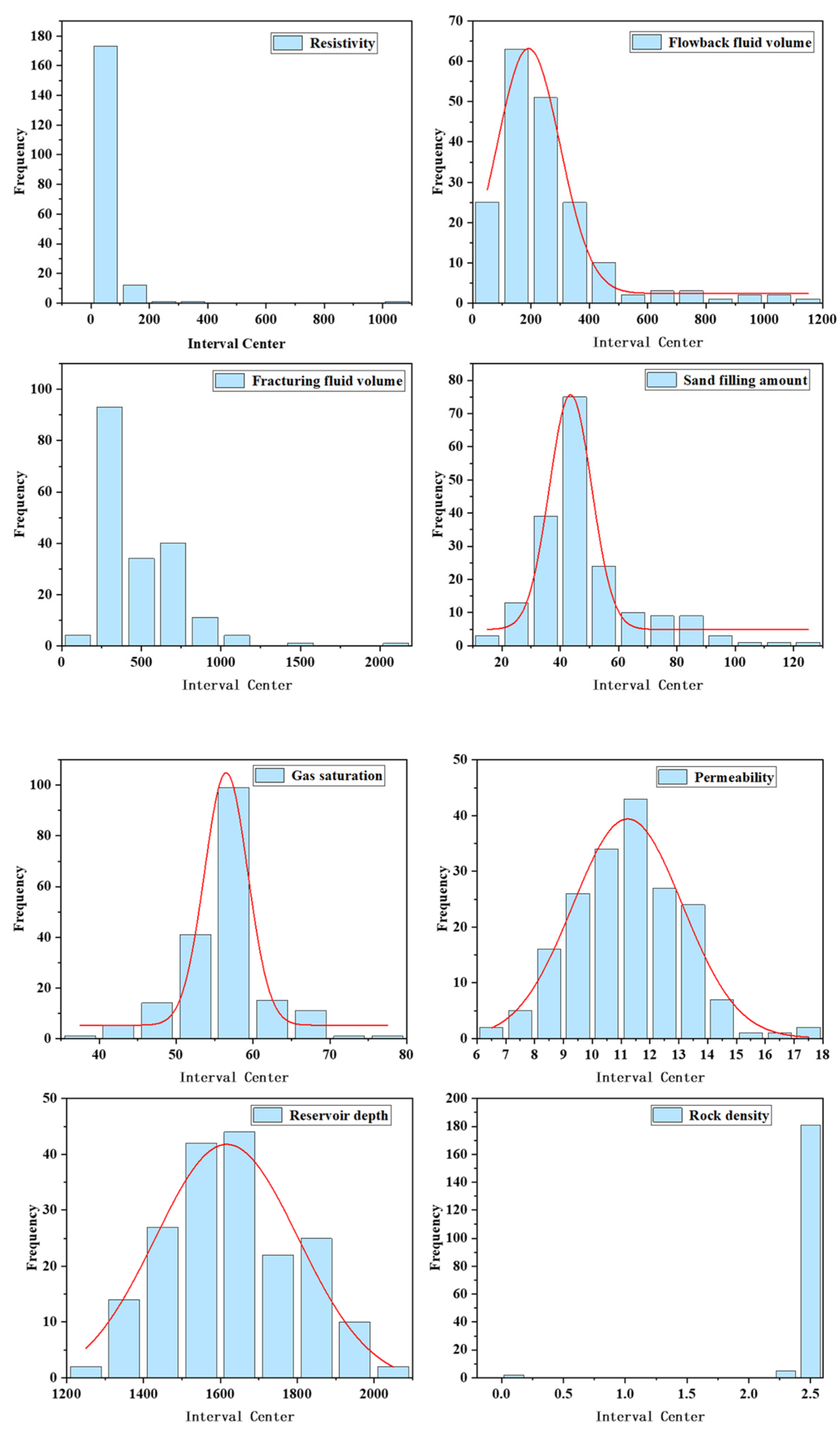
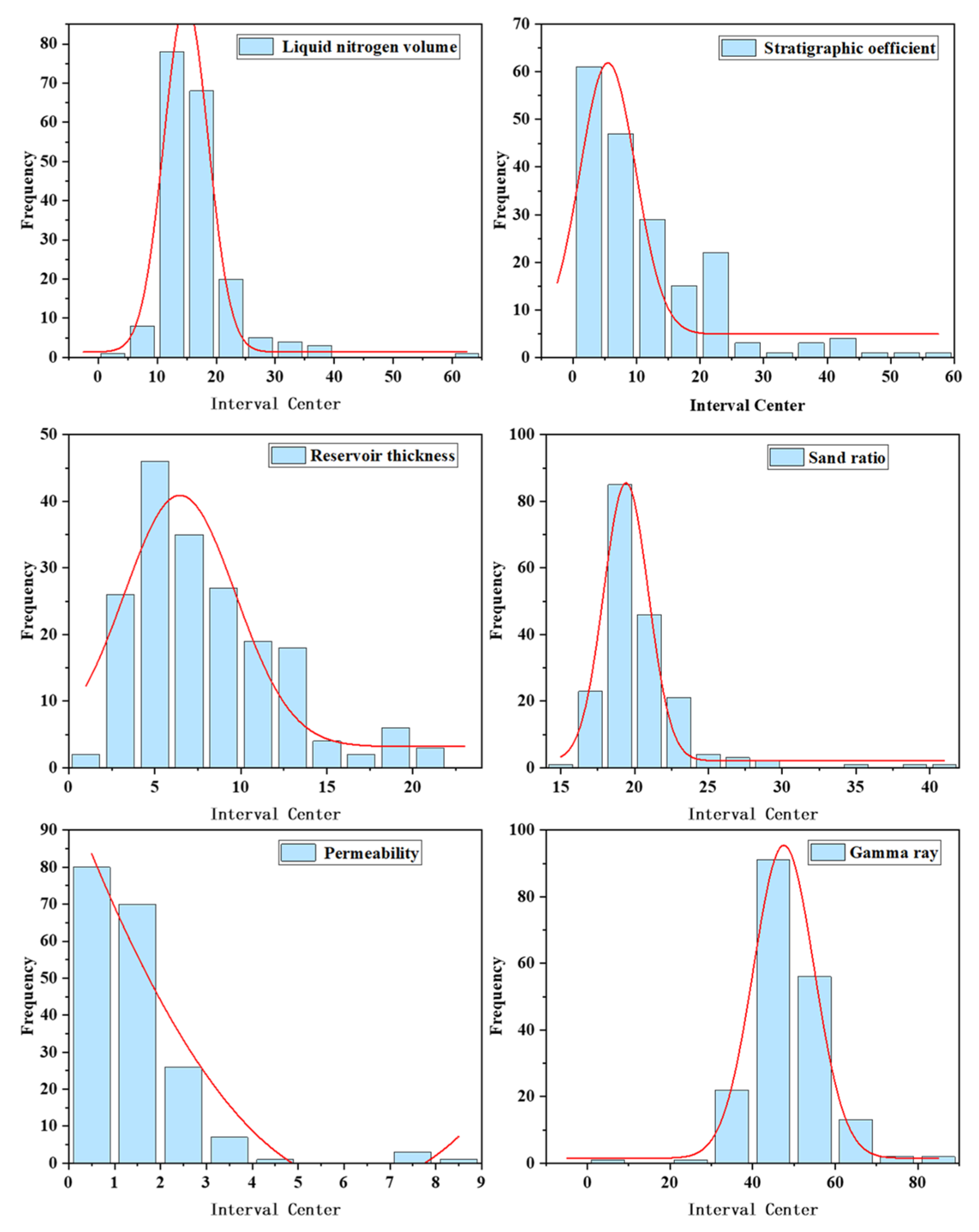
The training dataset includes 14 parameters for this machine learning application, which are gas saturation, stratigraphic coefficient, flowback fluid volume, reservoir thickness, permeability, porosity, gamma-ray, rock density, resistance, reservoir depth, liquid nitrogen volume, sand ratio, fracturing fluid volume, and sand filling amount. The distribution of each parameter in the training dataset is shown in Figure 1. The red line represents the trend of data distribution.
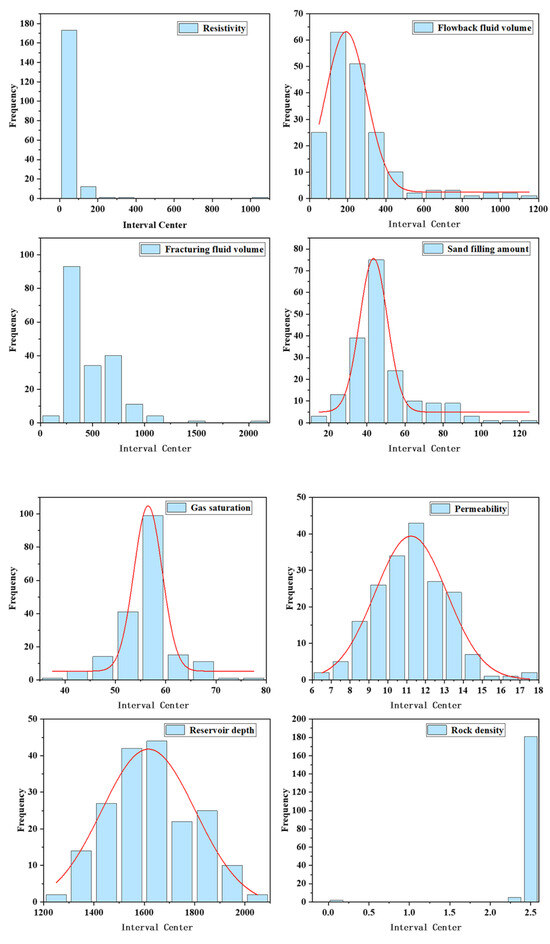
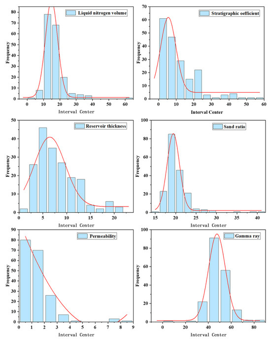
Figure 1.
Data distribution.
2.2. Correlation Analysis
Pearson, Spearman, and Kendall coefficients are all evaluated by the correlation coefficient as an indicator of the importance of factors, and their values are between −1 and 1. The variables have a positive correlation when the correlation coefficient is positive. The closer the value of the coefficient to 1, the stronger the positive trend. As the correlation coefficient is negative, the variables show a negative trend. The negative correlation is intense, as the coefficient value is close to −1. However, there is no correlation between the variables when the coefficient value equals 0. The equations of the three algorithms are presented as follows:
where is the variable corresponding to different values, is the mean of the variables, is the different values corresponding to the variables, is the average value of the variables, and is the number of variables.
where is the number of factors, and are the differences in the rank of each set of data.
where is the pair of elements with consistency in the data set and is the number of elements with inconsistency in .
2.3. Machine Learning Model
2.3.1. Support Vector Regression
Support vector regression (SVR) is a machine learning algorithm proposed by Vapnik et al. in the 1990s [26]. It has been extended to solve the complex linear indivisibility of data and “dimensional catastrophe” problems. The core methodology of SVR is mapping the sample data using the kernel function to a suitable high-dimensional characteristic space to realize the nonlinear analysis for the original data and determine the optimal hyperplane based on the mathematical derivation. Kernel functions are critical parameters of SVR, showing different sensitivities for various data categories. The typical kernel methods include linear, polynomial, Sigmoid, and radial [27]. In this paper, radial-based kernel functions are used for the SVR algorithm.
2.3.2. Back Propagation Neural Network
The backpropagation (BP) neural network algorithm was first proposed by Rumelhart and McClelland (1986) and employed to train multilayer perceptron feedforward neural networks according to the error backpropagation algorithm [28].
The BP neural network first performs forward propagation. Input data is passed through the input layer to the hidden layer, where it undergoes a series of weighted summations and activation function processing to produce the output of the hidden layer. This output is then transmitted to the output layer, where similar processing yields the final predicted output. Simultaneously, the predicted output is compared to the actual output, resulting in an error. The model then backpropagates this error, utilizing gradient descent to adjust the weights and biases of each connection in the network. This iterative process continues until reaching the maximum number of iterations or the error falls below a predefined threshold. BP primarily consists of an input layer, hidden layer, and output layer, which are fully connected. Nonlinear data infinitely fits when the hidden layer part is more than three layers under the influence of the activation function. The activation function is a non-linear function applied to the output of hidden layers in neural networks, aiming to introduce non-linear features and enhance the network’s expressive capability. It plays a crucial role in the performance and convergence speed of neural networks. ReLU function is a commonly used choice, effectively alleviating issues like gradient vanishing (it is used in this paper). In addition, the BP neural network has recently been gradually employed in the field of well productivity prediction. Compared to traditional prediction methods, it shows strong nonlinear mapping, universality, and fault tolerance capability. The BP neural network is an efficient and straightforward productivity prediction method.
2.3.3. Random Forest Regression
Random forest (RF) regression is an integrated algorithm combined with the Bagging method as the core and decision trees as the base learner. The RF model consists of multiple regression decision trees [29]. The nodes of each regression decision tree are divided by impurity-based features. A set of if-else structures is formed from the training set. Consequently, the regression values are output through the leaves. The final results are obtained by averaging the output results of all decision trees [30]. In addition, the random forest algorithm has a strong advantage in dealing with high-dimensional data and is simple to operate, fast to compute, and resistant to overfitting. The random forest algorithm is calculated using the following equations:
where is the data label value in the dataset, are two subsets after splitting, are the average value of data labels in subsets, are the number of data in subsets, is the cut point feature variable value, and is the order of characteristic sequence.
2.3.4. Grid Search Method
The grid search method is the most widely used technique to identify the optimal hyperparameter for a machine learning model. It determines the optimal value by calculating all hyperparameter combinations of the model. Generally, a larger range and smaller step size are used to determine the optimal global value, but it works only for numerical class parameters, not for classification parameters (e.g., internal kernel, etc.).
2.3.5. K-Fold Cross-Validation
K-fold cross-validation is a commonly used model evaluation technique. It divides the dataset into k mutually exclusive subsets, where one subset serves as the validation set and the remaining k-1 subsets serve as the training set. Then, the model is trained on these k-1 training sets and evaluated on the withheld validation set. This process is repeated k times, each time choosing a different validation set. Finally, the evaluation results from k iterations are averaged to obtain the final model performance assessment. K-fold cross-validation allows for more accurate model performance evaluation and reduces biases caused by uneven data distribution or single partitioning.
2.3.6. Confidence Interval
The confidence interval provides a reasonable range of values for a population parameter, allowing us to quantify the uncertainty associated with our estimate. Instead of providing a potentially misleading point estimate, confidence intervals give a range within which the true parameter value is likely to fall.
The results of 10-fold cross-validation form a dataset, where represents each data point in the dataset, denotes the standard deviation of the dataset, denotes the mean of the dataset, and represents the number of samples.
2.3.7. Summary of This Section
The above mentioned BP neural network adjusts the parameters of the neural network through forward and backward propagation; Random Forest builds multiple decision trees and integrates their prediction results; and Support Vector Machine finds the optimal hyperplane through kernel function transformation and maximal margin maximization. These different computational perspectives endow these three models with unique characteristics and applicability in handling data. This article aims to compare and select the best production capacity prediction model among them.
3. Productivity Prediction of Tight Gas Wells
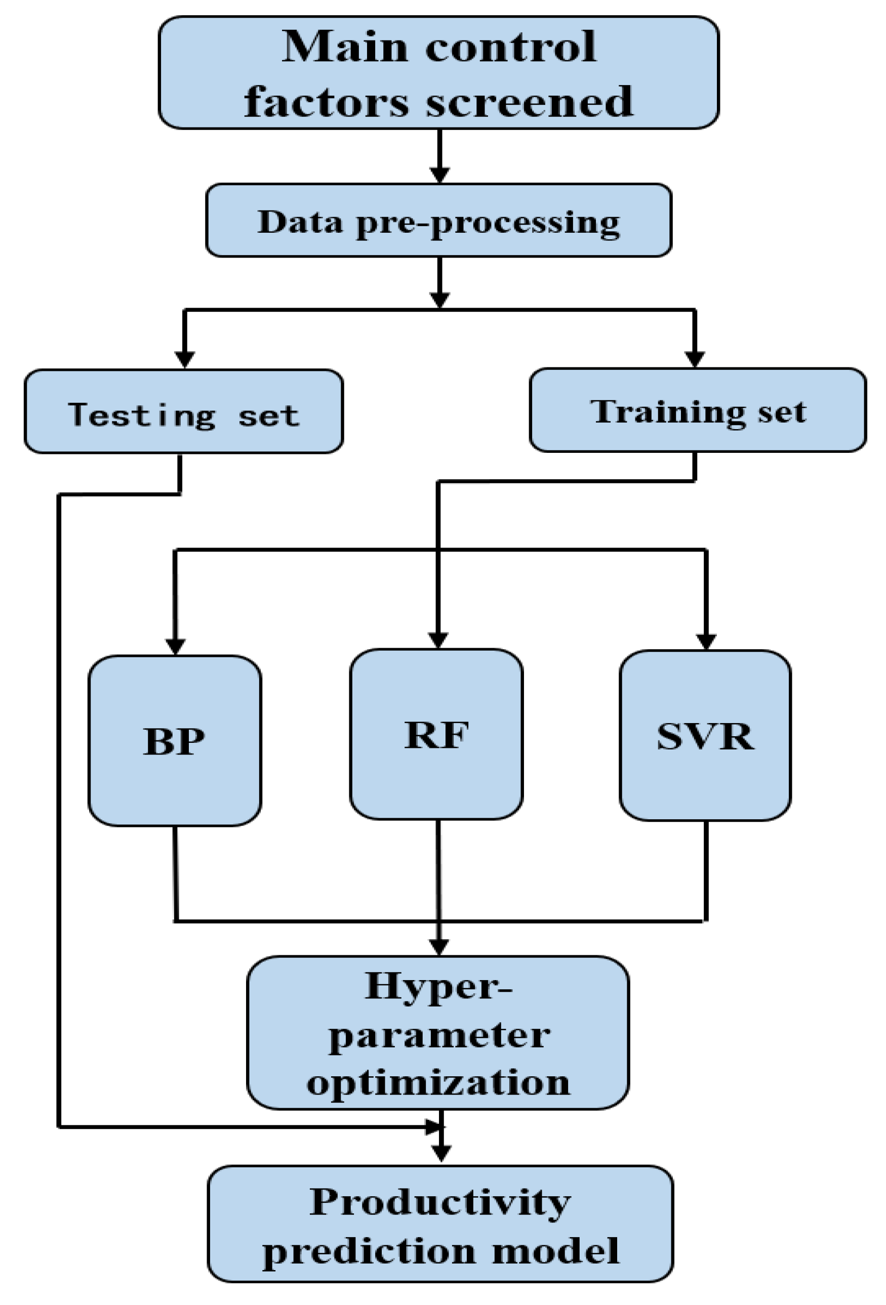
The research of the absolute open flow prediction models is carried out based on the algorithm of machine learning models. The primary workflow includes the following: (1) Pre-process data, and the dominant controlling factors as model input are screened by correlation analysis. The data from 170 wells are assigned as a training set, and the data from 19 wells are designated as the test set. (2) Based on the training set, BP, RF, and SVR models are employed to construct the base model. The hyper-parameters of the model are optimized by the grid-search method to achieve the best model training results. (3) The universality and accuracy of the models are examined by the test training set. The experimental flow chart is shown in Figure 2.

Figure 2.
Flow chart of the productivity forecasting model.
3.1. Correlation Analysis Results
The dimensions of the selected dominant controlling factors are different among the models, resulting in more considerable differences in the regression coefficients during the regression task. Normalization refers to the induction and unification of the probability distribution of the sample between zero and one [31]. The accuracy of the prediction model is affected, reducing the overall universality; therefore, it is essential to normalize the data before employing machine learning models. In this paper, the min–max normalization method is used to process the field data, effectively improving the model prediction accuracy. The equations related to the normalization process are presented below:
where is standardized data, is the original data, is the minimum value in the original data, and is the maximum value of the original data.
Currently, the analysis methods of productivity influencing factors mainly include experiments, numerical simulations, and analytical models [32,33,34]. The research is complex and time-consuming, meaning it cannot fulfill the fast and efficient requirements of field production. Therefore, Pearson, Spearman, Kendall, three methods of correlation analysis, and mathematical statistics are systematically employed to analyze the correlations between 14 parameters and absolute open flow. The optimal productivity controlling factors are screened under the constraint of gas reservoir engineering theories.
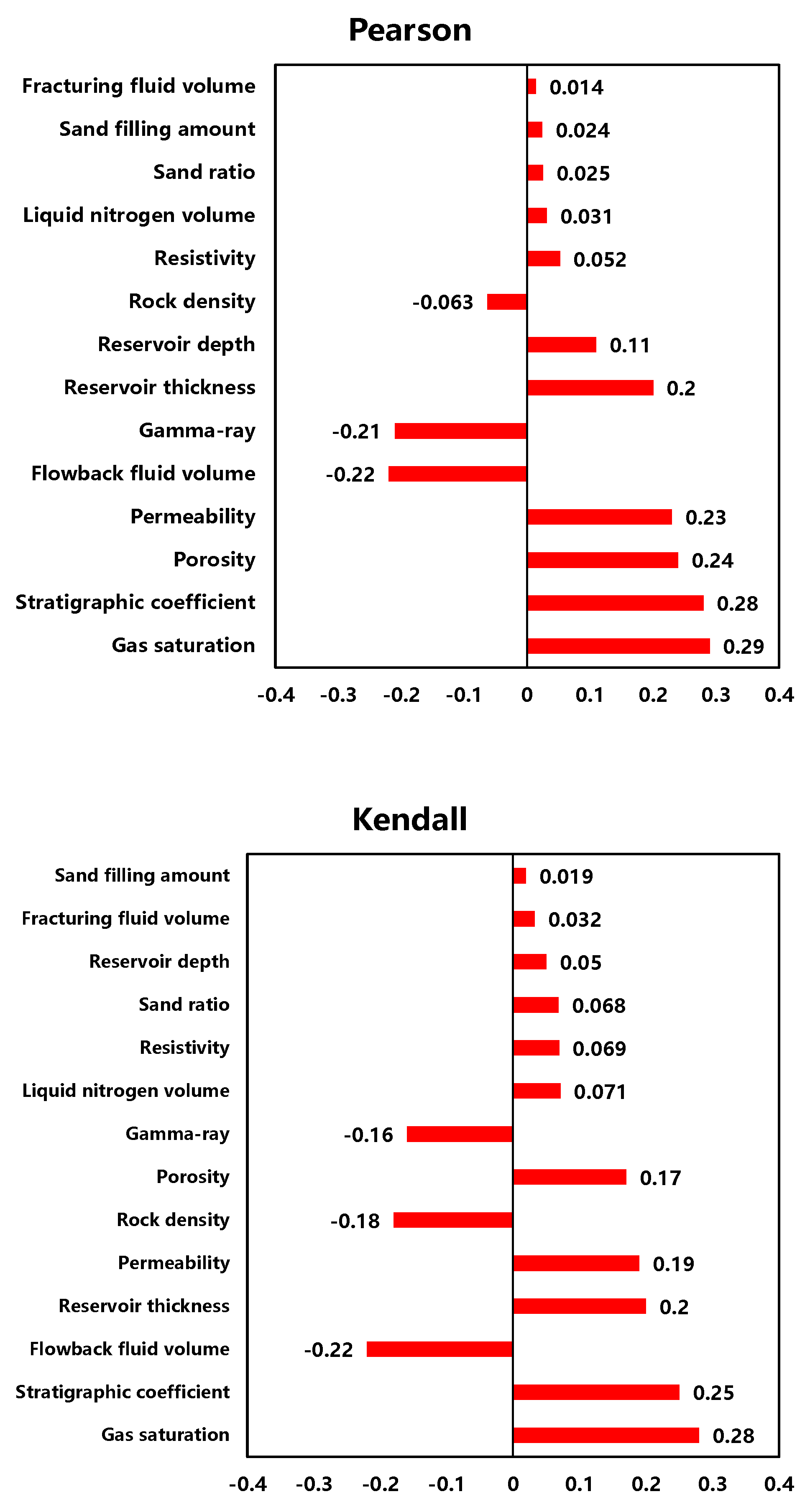
The results of correlation analysis using three algorithms are shown in Figure 3. The Spearman and Kendall methods achieve similar results, but Pearson has different results compared to the other methods. Since these algorithms possess various methodologies and strengths, the final ranking of controlling factors selects the average ranking of all three algorithms. The results are listed in Table 2.
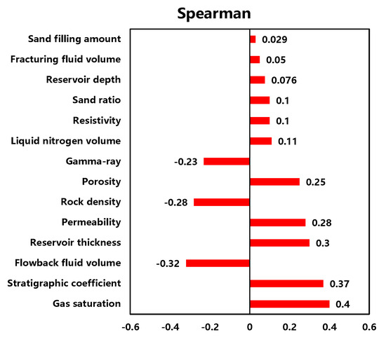

Figure 3.
Correlation analysis results of Spearman, Pearson, and Kendall.
Table 2.
Correlation ranking of influencing factors of production capacity.
From Table 2, reservoir characteristic parameters are more critical than fracturing parameters concerning well productivity for all three methods. Sand ratio, fracturing fluid volume, and proppant volume have a weak correlations with productivity. The highest degree of importance for productivity is gas saturation. Reservoir parameters, such as permeability and porosity, are more dominant than reservoir depth due to the complex geological structure of the Linxing gas field. Linxing gas reservoirs are characterized by high heterogeneity, severe gas seepage, and similar fracturing operations. It is essential to enhance the reservoir description of the gas reservoirs, and sweet spot studies should be carried out during the reservoir development stage. In addition, the results indicate that there is a strong correlation between the flowback fluid volume and productivity. The gas production decreases as flowback fluid volume increases, which can be used as a basis for productivity determination. Flowback fluid volume cannot be used as an input to the prediction model of this paper, as it is only obtained after the gas wells turn to production. It is generally acknowledged that correlation coefficients between −0.1 and 0.1 indicate no correlation. The article employs three methods for evaluation. Consequently, factors for which all three methods yield results within a range from −0.1 to 0.1 are eliminated. However, if one method yields a correlation result outside this range, the corresponding feature is selected. Based on these principles, 10 parameters of gas saturation, stratigraphic coefficient, reservoir thickness, permeability, porosity, gamma ray, rock density, resistivity, reservoir depth, and liquid nitrogen volume are selected as productivity prediction-related parameters for gas wells in the block.
3.2. Model Building and Hyper-Parameter Optimization
In this paper, the Keras library and Sklearn library of Python are used to develop BP, RF, and SVR models, and the grid-search method is employed to optimize hyperparameters of models based on the training set. The ranges of experimental parameters are presented in Table 3.
Table 3.
Range of experimental parameters.
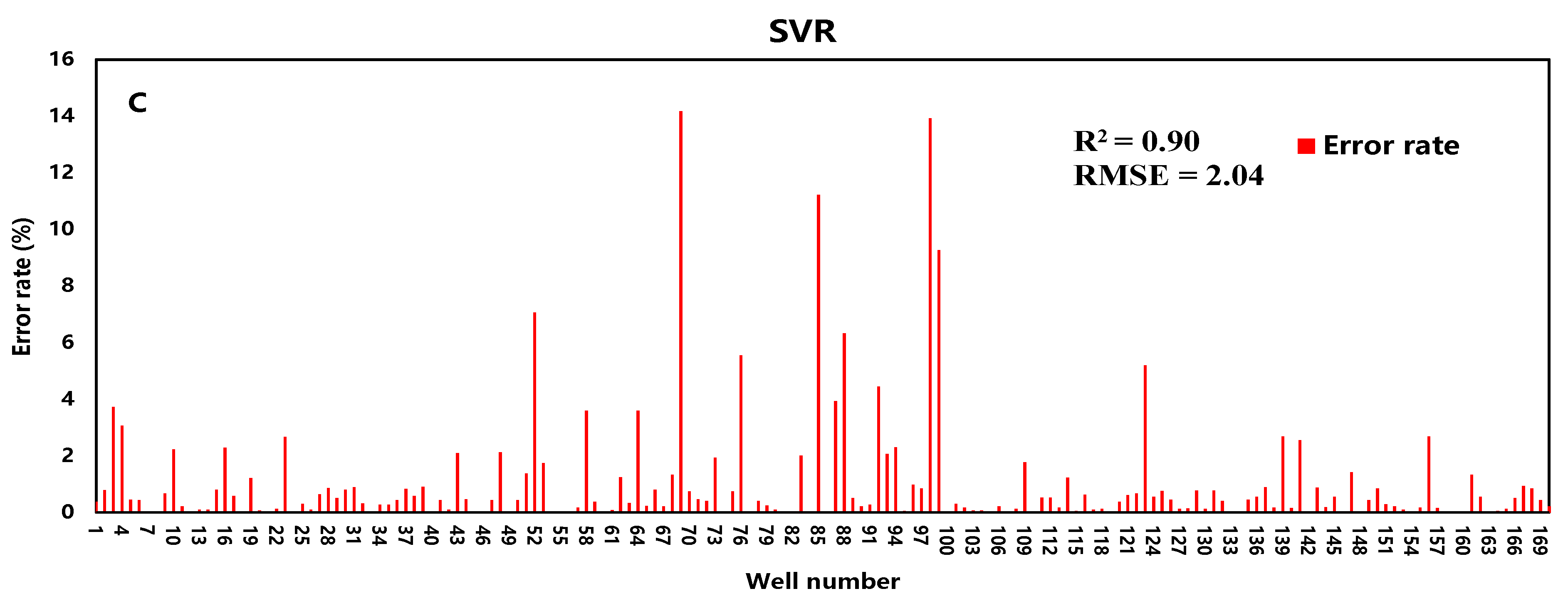
The grid search method optimizes the random forest model to determine the best combination of parameters: n_estimators are 140, max_depth is 10, and max_features are 0.1. The BP neural network model is determined to have six hidden layers, and the hidden unit sizes are 30, 50, 80, 120, 80, and 50, respectively. Epochs are 500 times, and the batch size is 100. The best combination of hyper-parameters for SVR is kernel function rbf, C 50, and gamma 0.06. We use the training dataset considering RMSE, R2 and Error Rate() indexes to examine and screen the models.
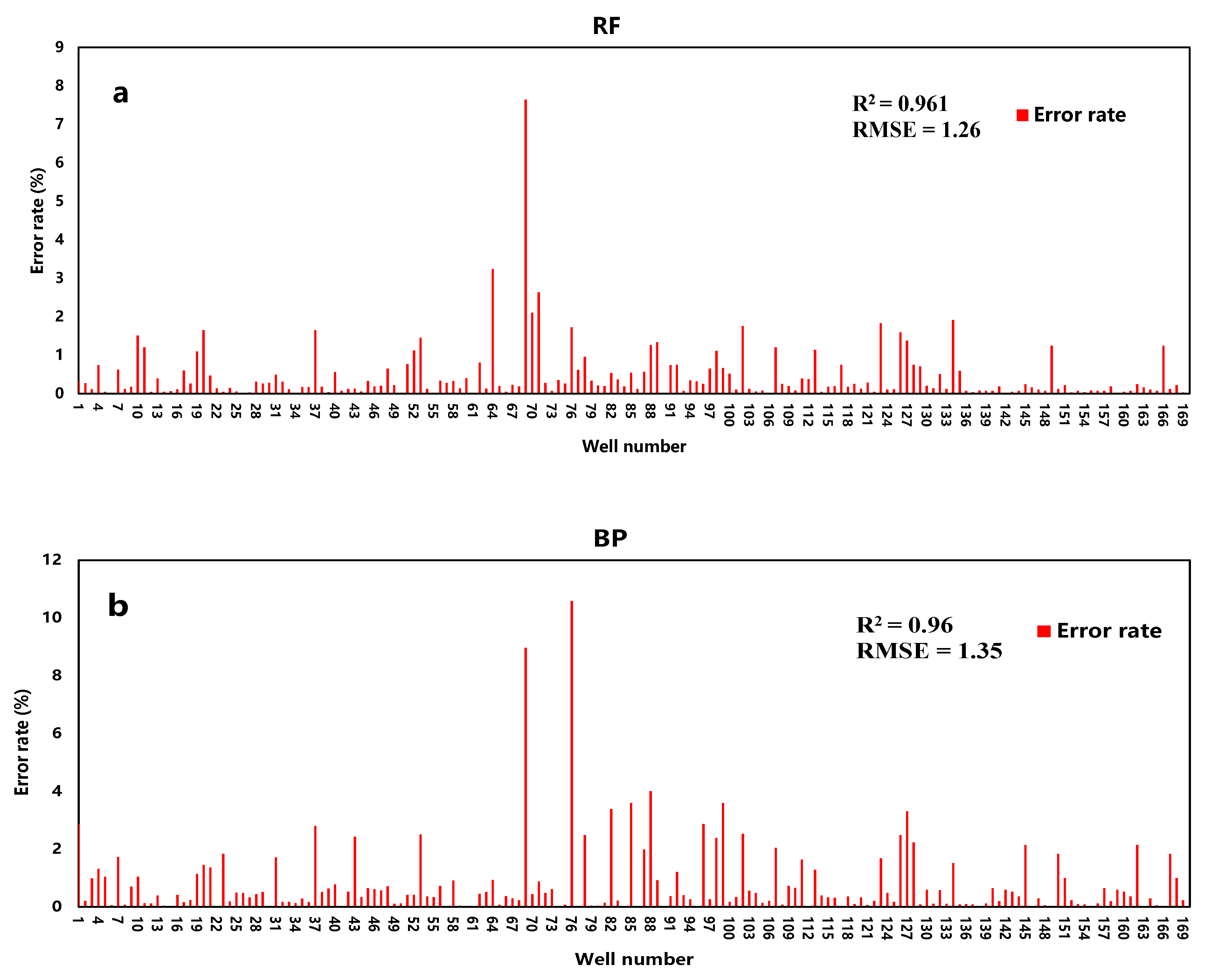
The R2 of the three models are 96.1%, 96%, and 90%, respectively. Although the accuracy of the SVR is slightly worse, it still is in good agreement with actual data. The fitting results are shown in Figure 4.
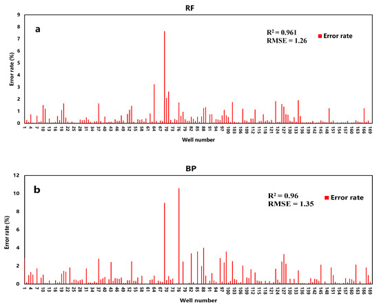
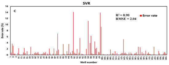
Figure 4.
Training accuracy of RF (a), BP (b), and SVR (c).
3.3. K-Fold Cross-Validation
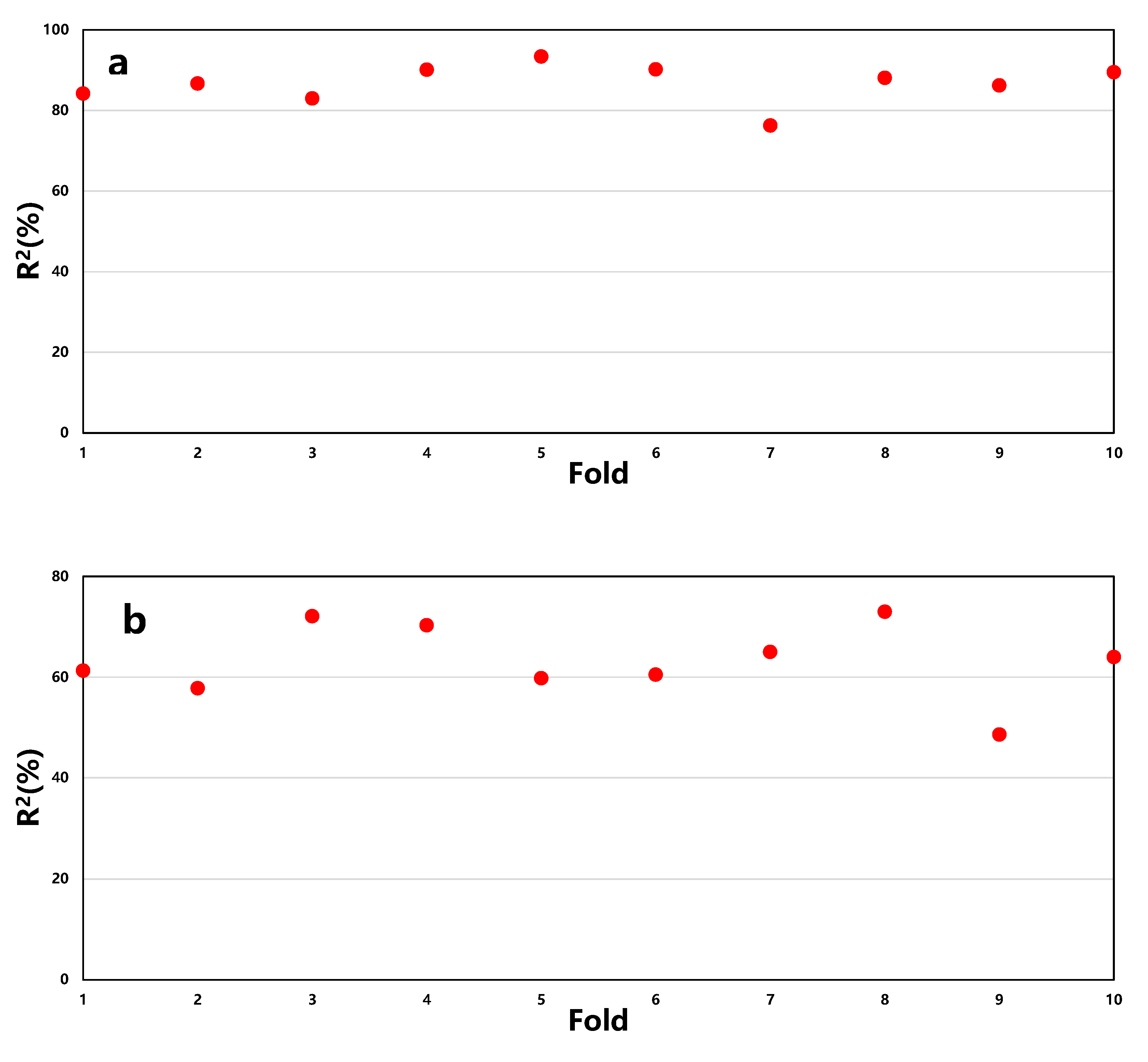
Based on the above hyperparameter settings, the article employs a k-fold cross-validation method to assess the stability of the model, with k set to 10, as shown in Figure 5.
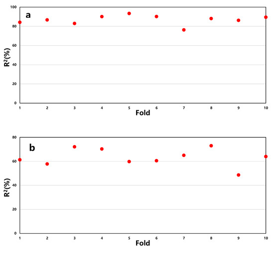
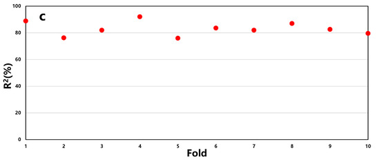
Figure 5.
The k-fold cross-validation results of RF (a), SVR (b), and BP (c) models.
From Figure 6, it can be observed that the average R2 for RF is 87%, SVR is 63%, and BP is 83%. Moreover, the stability of prediction accuracy for RF and BP is better compared to SVR. Therefore, it is concluded that the RF model demonstrates the best predictive performance.
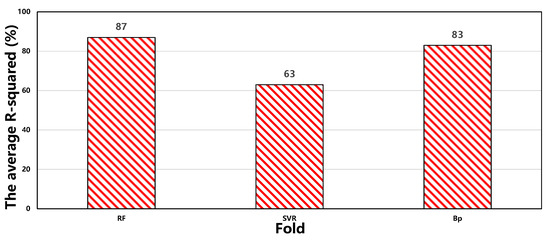
Figure 6.
Comparison analysis of three models.
3.4. Evaluation of Test Results
3.4.1. Comparative Analysis of Models
To prove the reliability of the prediction models and compare the adaptability and sensitivity of the three models for gas well data in this block, the prediction results are shown in Table 4 and Figure 7.
Table 4.
Errors of prediction results for three models.
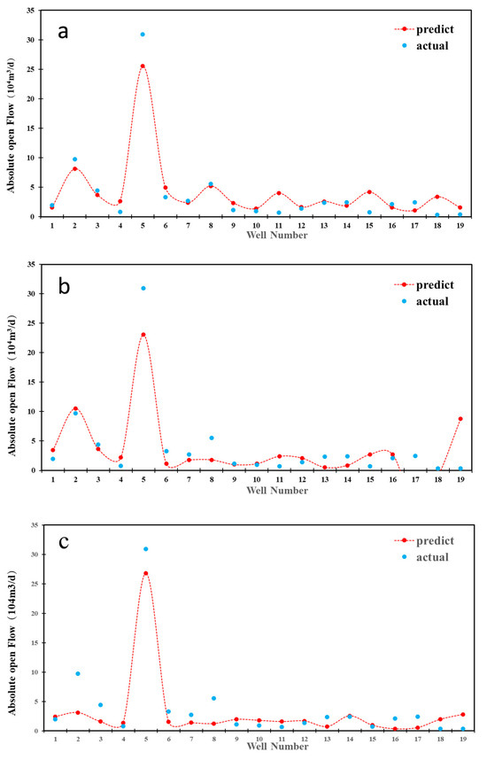
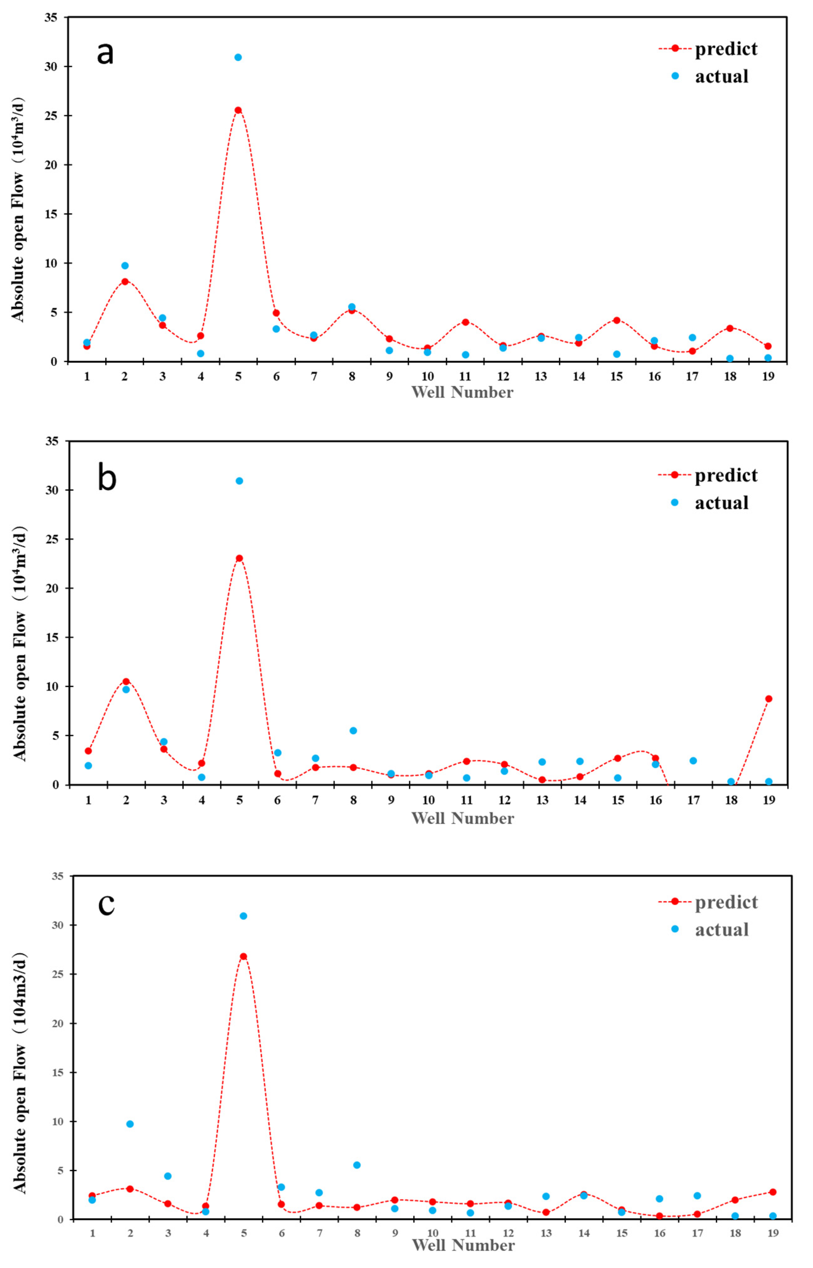
Figure 7.
Prediction results of RF (a), SVR (b), and BP (c) models.
From the results of the three models, the RF model with RMSE of 3.98 and R2 of 0.91 has the best adaptability from the perspective of machine learning. The prediction accuracy of the BP model is slightly worse than that of the RF model. The prediction error of the SVR model is the largest, in which the RMSE is 12.83 and R2 is 0.72. The prediction results of some wells are even negative values, indicating that the stability of the model is extremely poor.
During the actual production process, gas wells can be classified into low-producing, medium-producing, and high-producing wells, as various factors lead to differences in productivity. The test results demonstrate that the three models significantly differ in identifying various types of wells (as shown in Figure 7). The RF model entirely recognizes (100%) medium and high-producing wells, while the prediction effects of SVR and BP models are relatively insufficient. In addition, all three models inadequately distinguish low-producing wells because the critical factors of low-producing wells are more complex. It is challenging to effectively determine the productivity of low-producing wells from geological and fracturing parameters.
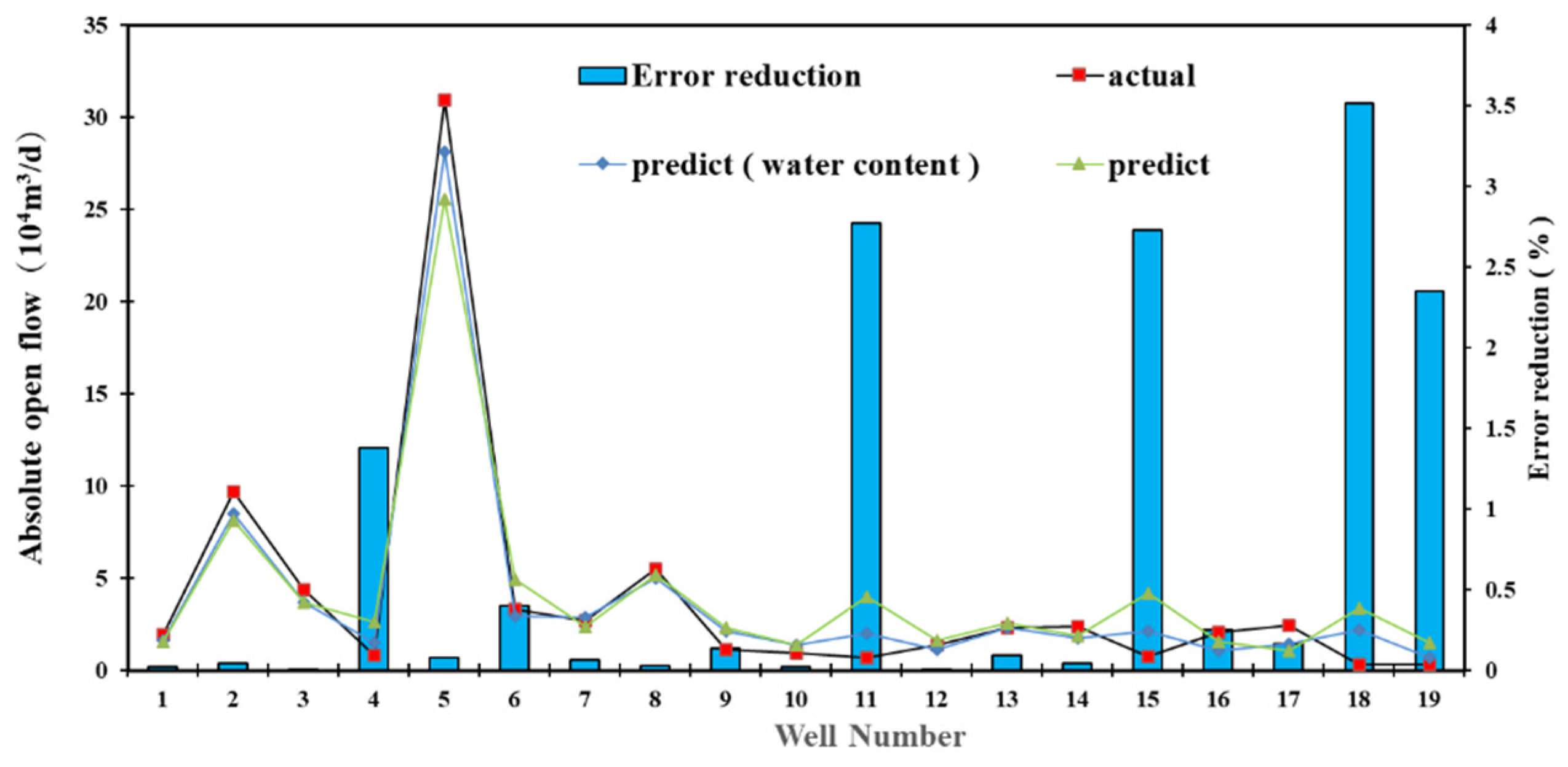
Due to the limitation of models on low-producing wells, the prediction models are re-verified using water production as an additional parameter. The results are presented in Figure 8. As the average daily water production of the gas well increases, the R2 of the RF prediction model is increased to 98.06%. The productivity prediction error of the low-producing well is significantly reduced, indicating the suppression of water accumulation in the wellbore on productivity. Therefore, the reliability of the prediction model is improved by adding water production as a parameter.
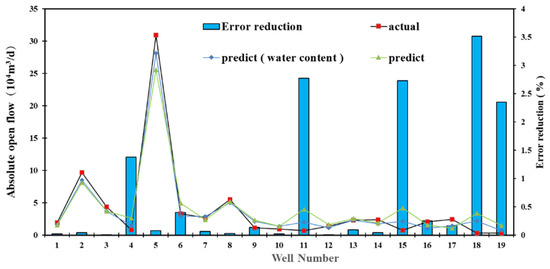
Figure 8.
Prediction results and error reduction range of model considering water production.
3.4.2. Confidence Interval Validation
In this study, we utilize the results of k-fold cross-validation to compute the confidence intervals for the test results of three models. The results are presented in Table 1.
From Table 5, it can be observed that only the prediction results of the SVR model in Section 3.4.1 fall outside the confidence interval range. This indicates that the SVR model is more sensitive to data variations compared to other models and has a weaker generalization ability; therefore, the SVR model shows the poorest adaptability for this study.
Table 5.
Confidence interval calculation results.
3.4.3. RF Model Validation
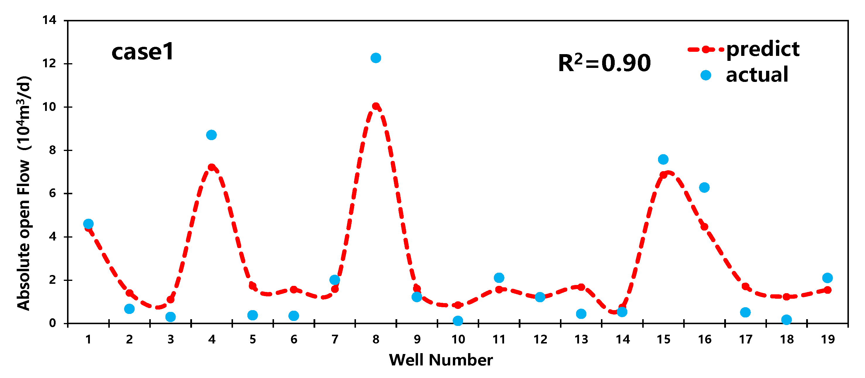
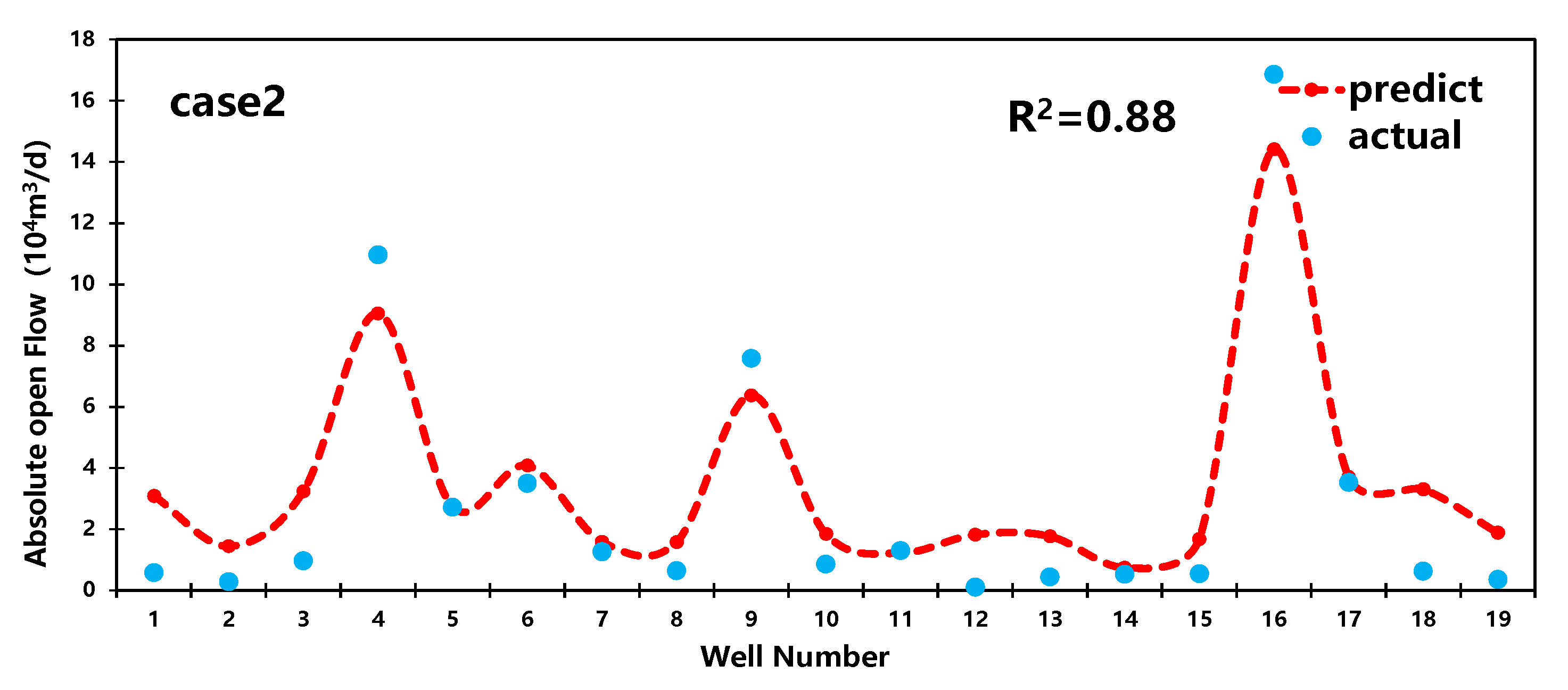
Based on the random forest regression model mentioned earlier in the text, the article randomly selects two additional sets of data for result analysis. The outcomes are illustrated in Figure 9.
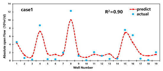
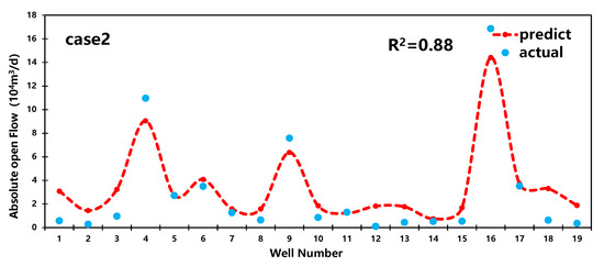
Figure 9.
Prediction results for case 1,2.
From Figure 9, it can be observed that the R2 values for the predictions of the two subsets by the RF model are 0.9 and 0.88, respectively. Additionally, the model demonstrates significantly higher prediction accuracy for medium-producing and high-producing wells compared to low-producing wells. Therefore, the random forest model is more suitable for predicting production capacity in medium-producing and high-producing wells.
3.5. Sensitivity Analysis
Based on the preferred random forest regression model mentioned above, a single-factor sensitivity analysis of the influencing factors on tight gas well productivity was conducted. Additionally, a physical consistency test method was employed to validate the model. Taking the data of one well as an example, the reliability of the model was further verified.
- (1)
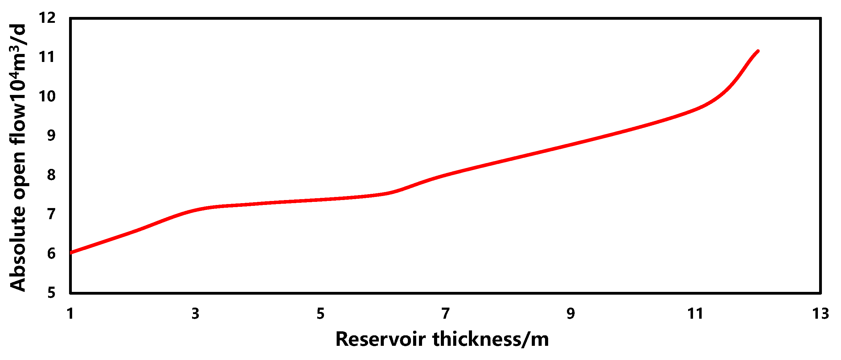
- Reservoir thickness
The sensitivity of the reservoir thickness in the production forecasting model is illustrated in Figure 10. Within a similar range, as the reservoir thickness increases, the gas well production capacity also increases, showing a positive correlation overall. This phenomenon indicates a greater reservoir thickness, with other parameters in the gas field remaining constant.
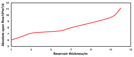
Figure 10.
The sensitivity of reservoir thickness.
- (2)
- Gas saturation
The sensitivity of the gas saturation in the production forecasting model is depicted in Figure 11. Within a similar range, as the gas saturation increases, the gas well production capacity also increases, exhibiting a positive correlation overall. This is primarily due to the fact that, with other parameters in the gas field remaining constant, higher gas saturation results in reduced flow resistance and improved flowability of gas within the reservoir, thereby favoring an increase in gas well production capacity.
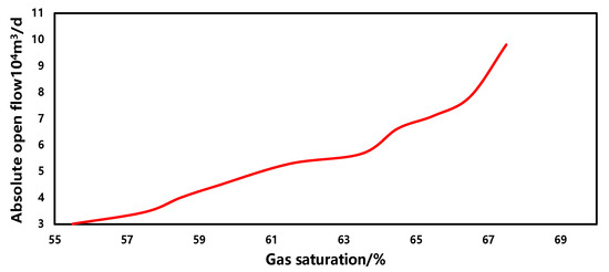
Figure 11.
The sensitivity of the gas saturation.
- (3)
- Stratigraphic coefficient
The sensitivity of the stratigraphic coefficient in the production forecasting model is illustrated in Figure 12. Within a similar range, as the formation coefficient increases, the gas well production capacity also increases, with a relatively large overall variation and a positive correlation. This phenomenon suggests that, when other parameters remain constant, a higher formation coefficient indicates a larger volume of gas stored in the reservoir and relatively less flow resistance within the reservoir, consequently leading to an increased gas well production capacity.
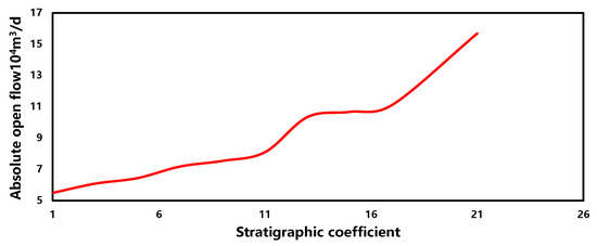
Figure 12.
The sensitivity of stratigraphic coefficient.
- (4)
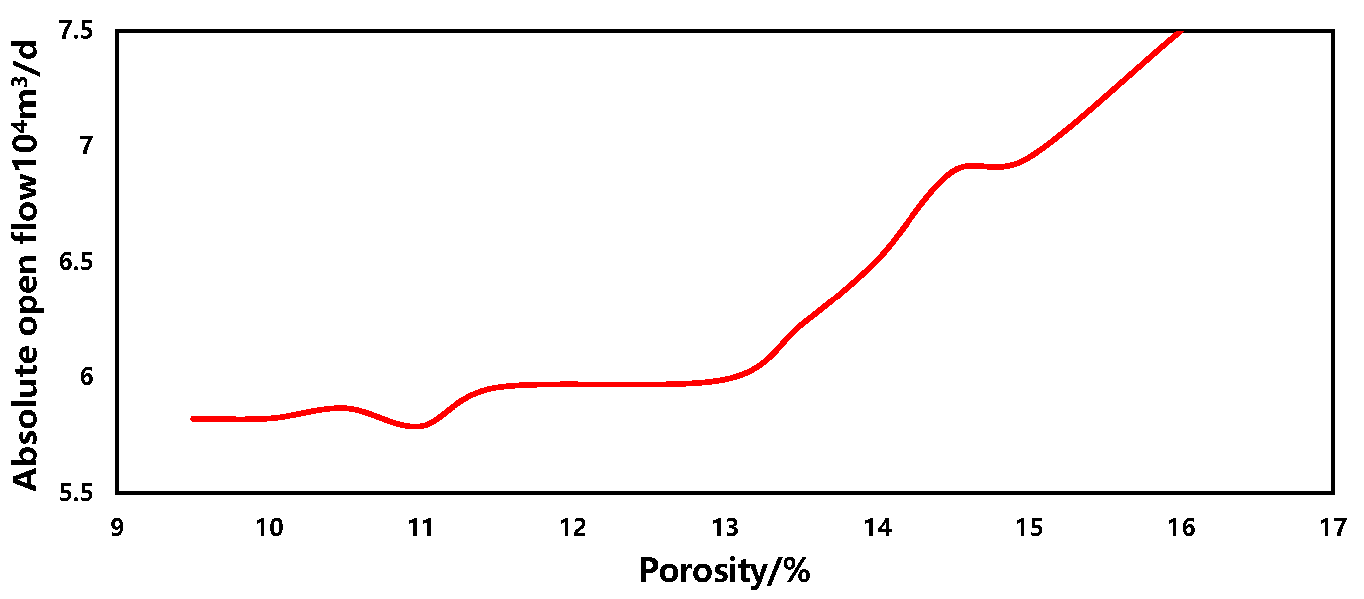
- Porosity
The sensitivity of the porosity in the production forecasting model is depicted in Figure 13. Within a similar range, as the porosity increases, the gas well production capacity also increases, showing a positive correlation overall. Furthermore, the positive correlation becomes more pronounced when the porosity exceeds 13. This phenomenon is primarily attributed to the increase in reservoir porosity, which enlarges the pore volume within the rock, allowing the reservoir to accommodate more gas and consequently increasing the gas well production capacity. However, as the porosity reaches a certain threshold, the rate of increase in gas well production capacity gradually diminishes because the rock pores are saturated. Further increases in porosity have less pronounced effects on gas well production capacity. Additionally, as porosity continues to increase to a certain extent, the connectivity between pores in the rock significantly improves, resulting in smoother pathways for gas flow and leading to a sudden increase in gas well production capacity.

Figure 13.
The sensitivity of porosity.
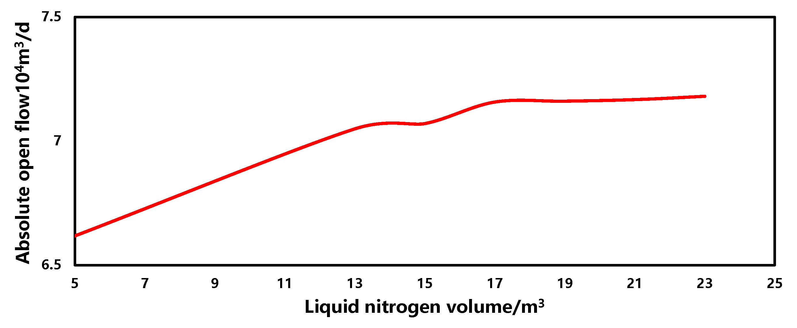
- (5)
- Liquid nitrogen volume
The sensitivity of the liquid nitrogen volume in the production forecasting model is illustrated in Figure 14. Within a similar range, as the liquid nitrogen volume increases, the gas well production capacity gradually increases, showing an overall positive correlation. However, when the liquid nitrogen volume reaches 17 m3, the production capacity stabilizes. This is primarily because liquid nitrogen is employed as a production enhancement measure to reduce bottomhole temperature, thereby reducing gas adhesion and condensation. However, as the liquid nitrogen volume increases, it permeates into the reservoir, leading to a decrease in reservoir permeability and restricting gas flow. Consequently, the effectiveness of production enhancement gradually diminishes.

Figure 14.
The sensitivity of liquid nitrogen volume.
- (6)
- Rock density
The sensitivity of rock density in the production forecasting model is depicted in Figure 15. Within a similar range, as the rock density increases, the gas well production capacity gradually decreases, showing an overall negative correlation. This phenomenon indicates that, with other parameters in the gas field remaining constant, a higher rock density results in smaller reservoir porosity and a smaller pore throat radius, leading to lower permeability of the reservoir. Consequently, the gas well production capacity is relatively lower.
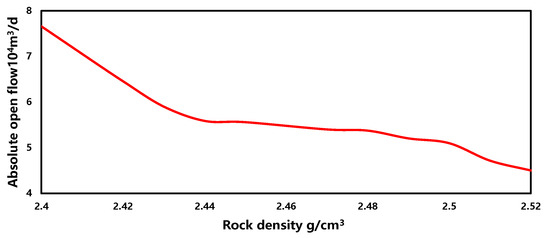
Figure 15.
The sensitivity of rock density.
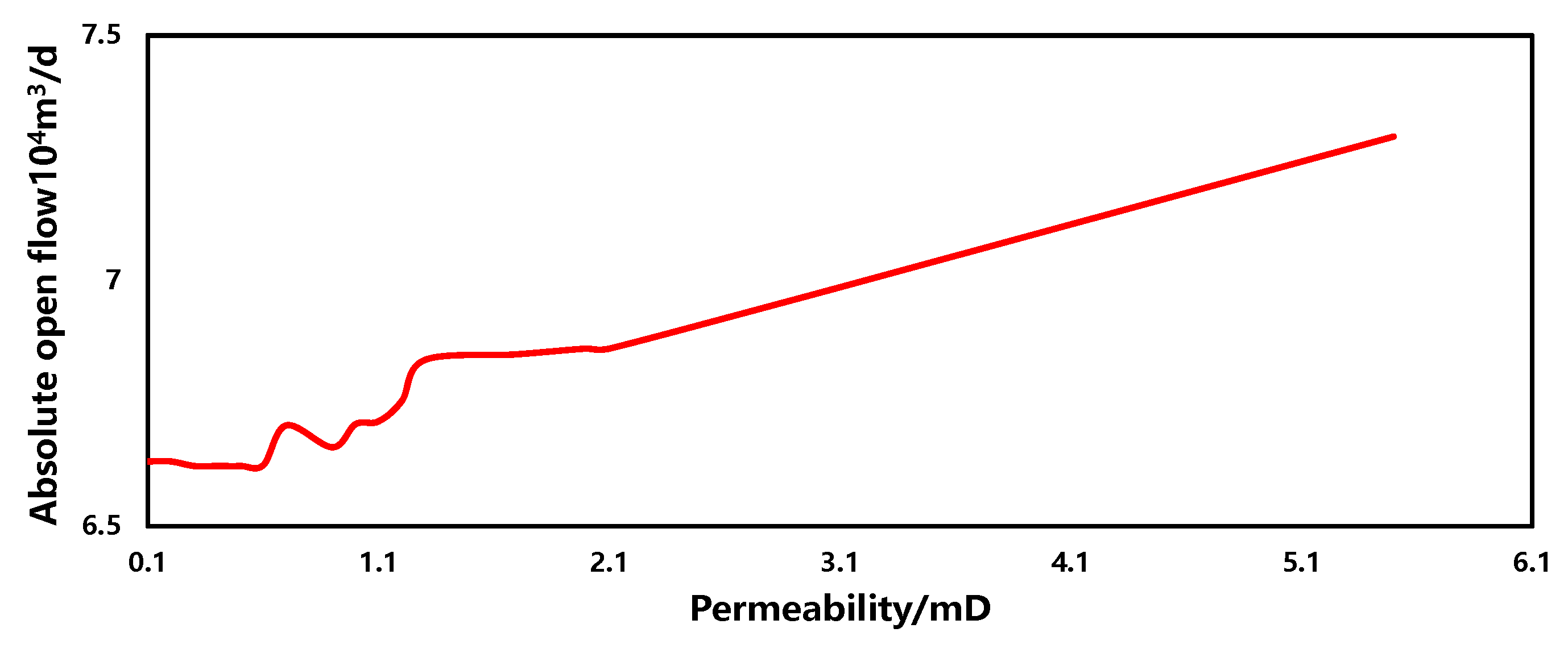
- (7)
- Permeability
The sensitivity of permeability in the production forecasting model is illustrated in Figure 16. Within a similar range, as the permeability increases, the gas well production capacity gradually increases, but the magnitude of change is relatively small. This phenomenon is primarily due to the extremely low initial permeability of tight gas reservoirs. Even with techniques such as hydraulic fracturing to increase permeability, the magnitude of increase remains relatively small. Therefore, under the constant conditions of other parameters, the impact of permeability on production capacity is not significant.

Figure 16.
The sensitivity of permeability.
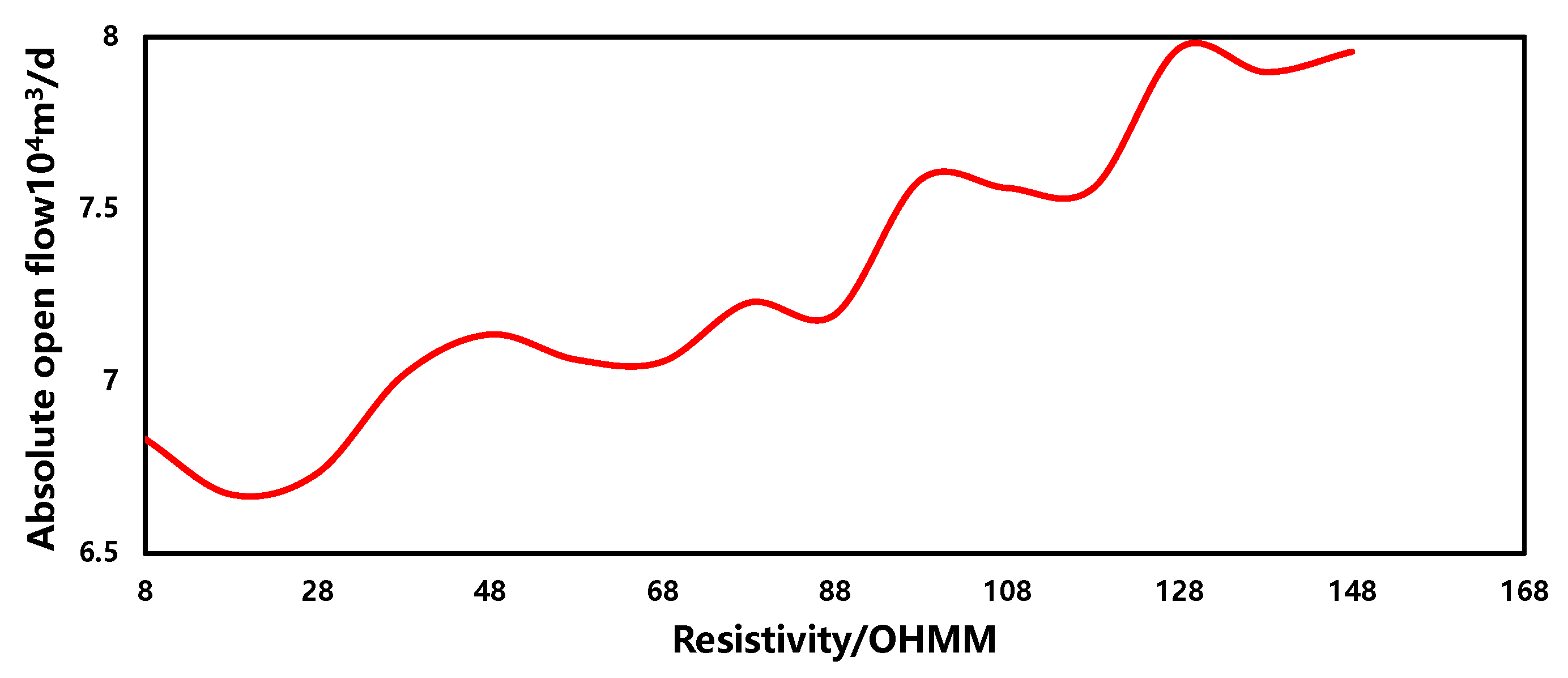
- (8)
- Resistivity
The sensitivity of resistivity in the production forecasting model is depicted in Figure 17. Within a similar range, as the resistivity increases, the gas well production capacity increases, showing a weak positive correlation overall, with fluctuations in the overall curve. This phenomenon is primarily due to the complex relationship between resistivity and gas well production capacity, which is not singular but may be influenced by multiple factors. Therefore, it requires comprehensive consideration and analysis.

Figure 17.
The sensitivity of resistivity.
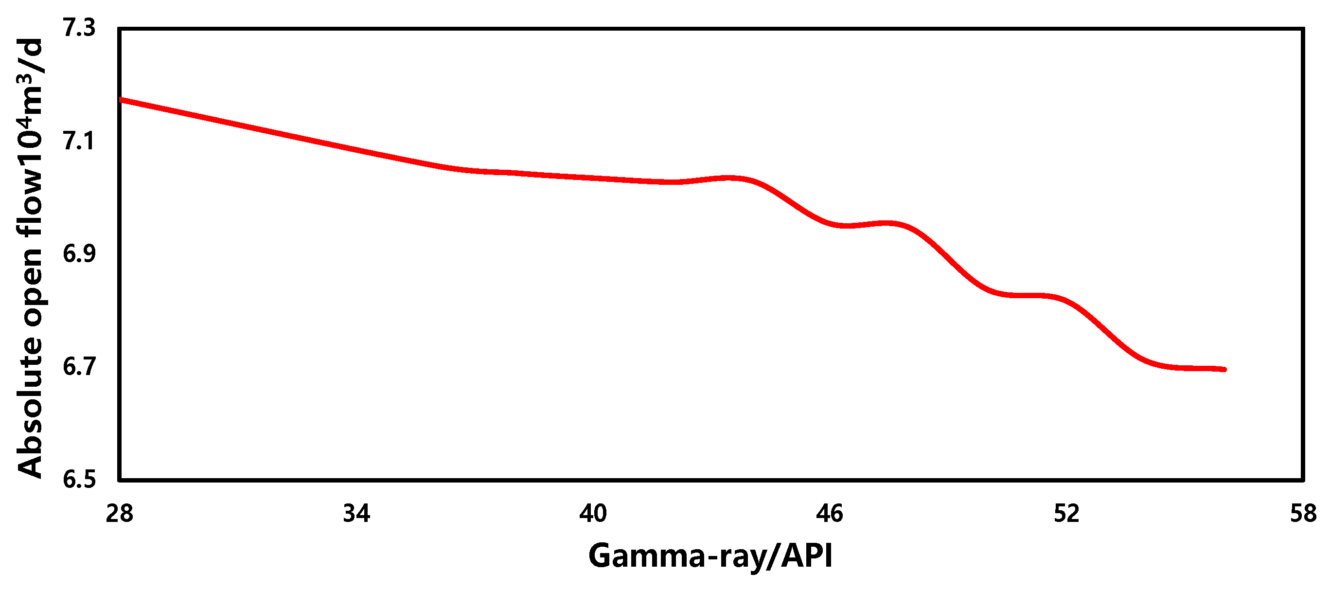
- (9)
- Gamma-ray
The sensitivity of the gamma-ray in the production forecasting model is illustrated in Figure 18. From the graph, it can be observed that, within a similar range, the change in production capacity is relatively small, showing an overall negative correlation. This phenomenon suggests that there is no direct causal relationship between natural gamma and gas well production capacity. Therefore, comprehensive analysis considering other parameters is necessary.

Figure 18.
The sensitivity of gamma-ray.
4. Model Application
Due to the highly heterogeneous gas reservoirs, the production systems and fracturing conditions between gas wells are different, resulting in significant differences in the recoverable reserves of gas wells in the Linxing field. Therefore, an effective method is needed to improve the estimation accuracy of EUR for gas wells. Typically, the prediction of single well recoverable reserves uses decline curve analysis combined with historical production data. This method is challenging in regard to determining the initial production for the unexplored area. In this study, a machine learning-based method is proposed for estimating single well recoverable reserve predictions based on geological and fracturing parameters in the early stages of gas well production.
4.1. Decreasing Curve Prediction
The gas wells in this block of Linxing are mainly characterized by high initial production and short stable production time. Typically, the Arps decline method is employed in the field to predict the EUR of a single well. Decline curve analysis is a classic method for predicting the production decline of oil and gas wells. The best-fitting model is selected based on the historical production data of the field. A characteristic of gas production in this block is a rapid production decline after a short period of constant production (control flow rate) and a stable production state (slow production decline), which generally satisfies the feature of hyperbolic decline. Therefore, the hyperbolic decline model is utilized to fit the gas production in the Linxing gas field and determine the features of gas production in this block.
Generally, the production potential for various gas wells is different, and the well type and well productivity can be classified based on absolute open flow rates. Based on the analysis of the decline rate of gas wells in the Linxing reservoirs, the original three types of gas wells are re-classified into four categories according to absolute open flow rate. Among them, the numbers of Type I, II, III, and IV wells are 42, 40, 30, and 15, respectively. The selected gas wells produced gas for more than 12 months and normalized the production during the decline stage. Then, the hyperbolic decline curve is used to fit the production of four types of wells to obtain typical decline curves. The cumulative gas production is used to evaluate the performance of curve fitting, as shown in Table 6 and Figure 19. Between the two red lines is the gas well depletion period.
Table 6.
Production parameters of classified gas wells.
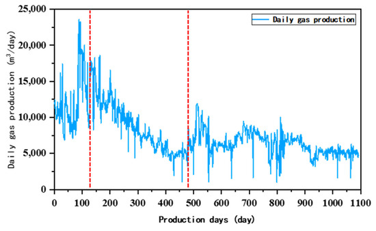
Figure 19.
Production performance of a gas well in this area.
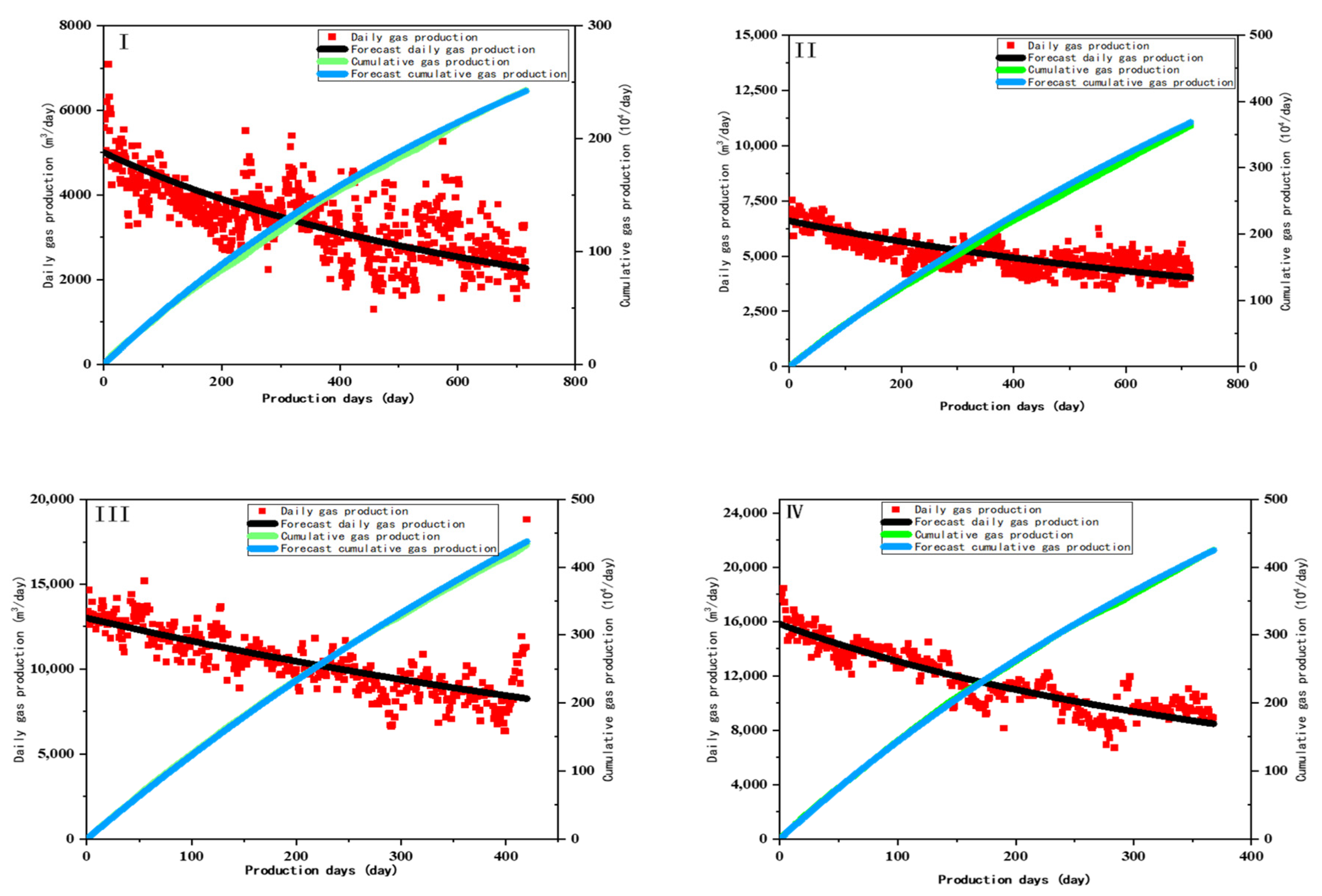
The fitting results of the gas production decline curve are shown in Figure 20. The production of Type I wells has the most significant fluctuation due to the rapid water breakthrough. In addition, water accumulation occurs in the wellbore in the early testing stage and repeatedly happens during the production stage. Foam drainage operation is a commonly used solution for resolving accumulated water in the wellbore problem, but the operation causes considerable gas production fluctuations.

Figure 20.
Fitting of the decline law of typical wells. (I) Typical decline curve of Type I well; (II) Typical decline curve of Type II well; (III) Typical decline curve of Type III well (IV) Typical decline curve of Type IV well.
I well hyperbolic decline fitting formula:
II well hyperbolic decline fitting formula:
III well hyperbolic decline fitting formula:
IV well hyperbolic decline fitting formula:
Type II wells have the smallest decline rate, followed by Type III and Type I wells. Type IV wells have the highest decline rate because the early production of these wells is assigned very high, resulting in insufficient energy supplies and a rapid decline in gas wells. Therefore, the ratio of the average open flow rate of each type of gas well to the initial production of the typical decline curve provides a more reasonable initial co-production basis for the site, as shown in Table 6.
4.2. RF Model Prediction
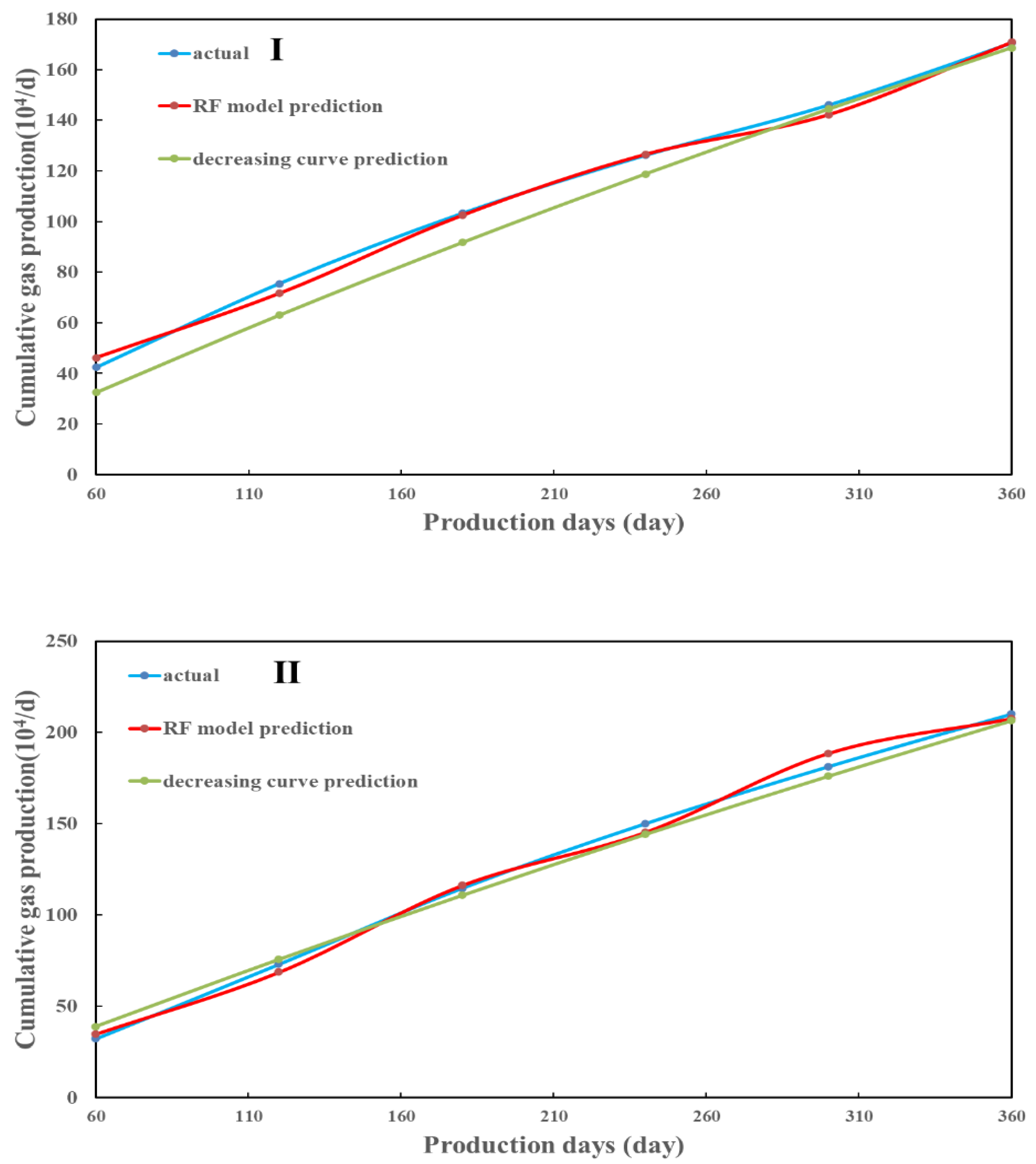
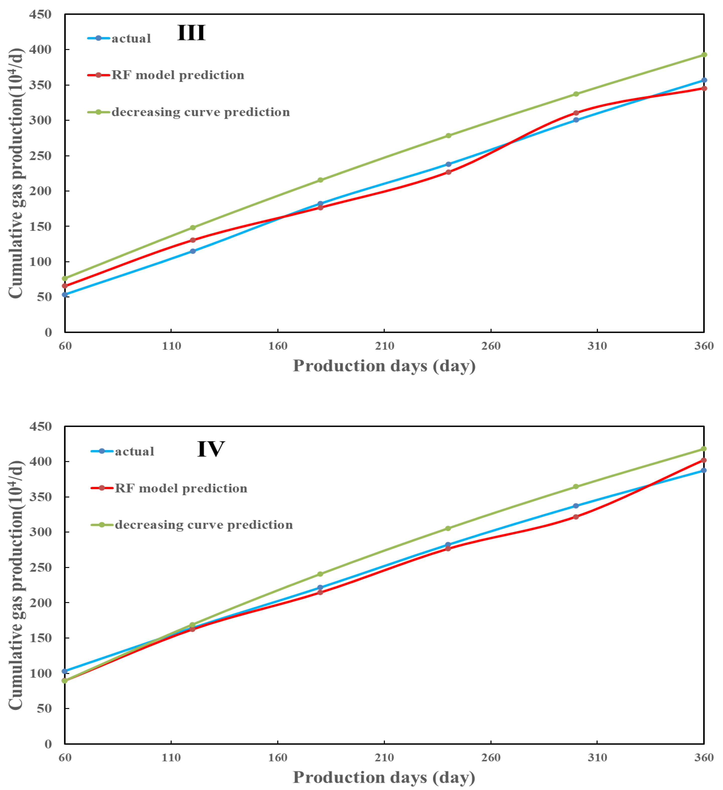
The initial and cumulative production correlation is established using the RF model to predict the cumulative production of the four wells at different stages (with two months as a stage) during the first 12 months. The results were compared with the prediction results of typical decline curves to evaluate the performance of machine learning in production prediction. Figure 8 shows the predicted 12-month cumulative production errors of Type I wells using the RF model, and the typical decline curve models are 0.07% and 1.12%, respectively. The prediction effect of the RF model is significantly better than that of the typical decline curve model. The errors of Type II wells for the two models are 1.17% and 1.65%, respectively, and the prediction results of the RF model are better agreed with the actual cumulative production trend. For Type III wells, errors are 3.2% and 10.08%, respectively, and the prediction results of RF are more dominant in each stage. The errors of Type IV wells for the two models are 3.8% and 7.9%, and the RF model is more accurate than the decline curve method. Therefore, we conclude that the prediction accuracy of the RF model is better than that of the typical decline curve model, which avoids the influence of the initial production error on the cumulative prediction. During actual gas production, various operations are often conducted in the field, resulting in output fluctuations during production. The decline curve cannot eliminate this difference, significantly impacting production forecasting. As shown in Figure 21, the prediction results of the machine learning model are more in line with the actual production.
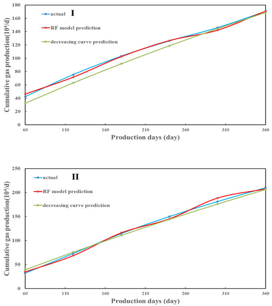
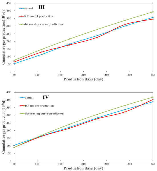
Figure 21.
Four types of typical well productivity prediction results. (I) Type I well prediction results; (II) Type II well prediction results; (III) Type III well prediction results; (IV) Type IV well prediction results.
4.3. EUR Prediction
The medium and high-producing wells (named Well−1, Well−3, and Well−5) are randomly selected from the database to predict 20-year EUR using two methods. As shown in Table 7, the absolute open flow rate of the gas well indicates the production potential of the well. Combined with the typical decline curve of different types of wells, the EUR of a single well can be predicted. The forecasted 20-year EUR for Well−1, Well−3, and Well−6 is 958.8 × 10⁴ m3, 1819.9 × 104 m3, and 4109.8 × 104 m3, respectively. Compared with the prediction results of OFM software (2014V2), the differences for the three wells are 9.9%, 13.7%, and 6.5%, respectively, and the differences are all within the acceptable range.
Table 7.
Prediction results and initial production of selected wells.
Oil Field Management (OFM) software predicts the recoverable reserves of a single well based on the historical production of wells. The proposed machine learning-based model can complete the prediction at the early stage of geological analysis. The method uses machine learning models to reveal the correlation between productivity with geological and fracturing parameters, as well as to predict the absolute open flow rate of gas wells. Combined with the typical decline curve, the model can predict the recoverable reserves of a single well, which provides an effective method for determining the productivity potential of gas wells and planning new wells. In the process of economical cost, the overall work efficiency is improved. As EUR prediction is completed before the production period, it provides insight into the surface facility and piping design to improve the project’s economics.
5. Conclusions
(1) The statistical analysis method can quickly determine the dominant controlling factors of well productivity and provide a quantitative evaluation. This study analyzes the performance of 10 parameters, including gas saturation, reservoir thickness, etc., on gas well productivity in this block. The results indicate that geological factors play a more significant role than fracturing factors in well productivity prediction.
(2) The RF model can accurately predict the absolute open flow of gas wells and distinguish the type of gas wells. Based on machine learning evaluation, the RF prediction model with an RMSE of 3.98 and R2 of 0.91 has the highest prediction accuracy, followed by the BP. The SVR model has the largest prediction error. From the practical application, the RF model entirely (up to 100%) recognizes the medium- and high-production wells. Therefore, the RF model is recommended for employment in productivity prediction in the Linxing gas reservoirs.
(3) The research shows that the deviation of the initial production leads to inaccurate prediction results regarding the typical decline curve. It is challenging for the typical decline curve to capture the character of actual production for the wells that conducted multiple operations. The 12-month cumulative production forecasting of the four wells using the RF model is more accurate than the typical decline curve model, verifying the applicability of machine learning in production prediction.
Author Contributions
Conceptualization, H.S. and M.F.; methodology, H.S.; software, H.S.; validation, H.L., H.S. and M.F.; formal analysis, H.S.; investigation, H.L.; resources, M.F.; data curation, M.F. and H.L; writing—original draft preparation, H.S.; writing—review and editing, H.S.; visualization, H.S.; supervision, T.L.; project administration, M.F.; funding acquisition, M.F. All authors have read and agreed to the published version of the manuscript.
Funding
This research received no external funding.
Data Availability Statement
The data are not publicly available due to the privacy restrictions of the company.
Acknowledgments
The authors would like to thank the CNOOC Research Institute for providing data support.
Conflicts of Interest
Authors Maojun Fang, Hengyu Shi and Hao Li were employed by the company CNOOC Research Institute Co., Ltd. The remaining authors declare that the research was conducted in the absence of any commercial or financial relationships that could be construed as a potential conflict of interest.
Nomenclature
| EUR | Estimated Ultimate Recovery |
| SVR | Support Vector Regression |
| RF | Random Forest |
| BP | Back Propagation |
| Pearson | Pearson’s correlation coefficient method |
| Spearman | Spearman’s correlation coefficient method |
| Kendall | Kendall’s correlation coefficient method |
| Spearman coefficient value | |
| Pearson coefficient value | |
| Kendall coefficient value | |
| C | The penalty coefficient |
| Linear | Linear Kernel |
| poly | Polynomial Kernel |
| rbf | Radial Basis Function |
| RMSE | Root Mean Square Error |
| R2 | Coefficient of Determination |
| OFM | Oil Field Management |
References
- Motiur Rahman, M. Productivity Prediction for Fractured Wells in Tight Sand Gas Reservoirs Accounting for Non-Darcy Effects. In Proceedings of the SPE Russian Oil and Gas Technical Conference and Exhibition, Moscow, Russia, 28 October 2008. [Google Scholar]
- Wu, Y.; Cheng, L.; Huang, S.; Fang, S.; Killough, J.E.; Jia, P.; Wang, S. A Transient Two-Phase Flow Model for Production Prediction of Tight Gas Wells with Fracturing Fluid-Induced Formation Damage. In Proceedings of the SPE Western Regional Meeting, San Jose, CA, USA, 22 April 2019. [Google Scholar]
- Aranguren, C.; Fragoso, A.; Aguilera, R. Sequence-to-Sequence (Seq2Seq) Long Short-Term Memory (LSTM) for Oil Production Forecast of Shale Reservoirs. In Proceedings of the SPE/AAPG/SEG Unconventional Resources Technology Conference, Houston, TX, USA, 20–22 June 2022. [Google Scholar]
- Biswas, D. Adapting Shallow and Deep Learning Algorithms to Examine Production Performance—Data Analytics and Forecasting. In Proceedings of the SPE/IATMI Asia Pacific Oil & Gas Conference and Exhibition, Bali, Indonesia, 25 October 2019. [Google Scholar]
- Kocoglu, Y.; Gorell, S.; McElroy, P. Application of Bayesian Optimized Deep Bi-LSTM Neural Networks for Production Forecasting of Gas Wells in Unconventional Shale Gas Reservoirs. In Proceedings of the SPE/AAPG/SEG Unconventional Resources Technology Conference, Houston, TX, USA, 26–28 July 2021. [Google Scholar]
- Le, N.T.; Shor, R.J.; Chen, Z. Physics-Constrained Deep Learning for Production Forecast in Tight Reservoirs. In Proceedings of the SPE/AAPG/SEG Asia Pacific Unconventional Resources Technology Conference, Virtual, 16–18 November 2021. [Google Scholar]
- Wu, T.; Fang, H.; Sun, H.; Zhang, F.; Wang, X.; Wang, Y.; Li, S. A Data-Driven Approach to Evaluate Fracturing Practice in Tight Sandstone in Changqing Field. In Proceedings of the International Petroleum Technology Conference, Virtual, 16 March 2021. [Google Scholar]
- Chunxin, W.; Shaopeng, W.; Jianwei, Y.; Chao, L.; Qi, Z. A prediction model of specific productivity index using least square support vector machine method. Adv. Geo-Energy Res. 2020, 4, 460–467. [Google Scholar]
- Vyas, A.; Datta-Gupta, A.; Mishra, S. Modeling Early Time Rate Decline in Unconventional Reservoirs Using Machine Learning Techniques. In Proceedings of the Abu Dhabi International Petroleum Exhibition & Conference, Abu Dhabi, UAE, 13 November 2017. [Google Scholar]
- Liao, L.; Zeng, Y.; Liang, Y.; Zhang, H. Data Mining: A Novel Strategy for Production Forecast in Tight Hydrocarbon Resource in Canada by Random Forest Analysis. In Proceedings of the International Petroleum Technology Conference, Dhahran, Kingdom of Saudi Arabia, 13 January 2020. [Google Scholar]
- Han, D.; Kwon, S.; Kim, J.; Jin, W.; Son, H. Comprehensive Analysis for Production Prediction of Hydraulic Fractured Shale Reservoirs Using Proxy Model Based on Deep Neural Network. In Proceedings of the SPE Annual Technical Conference and Exhibition, Virtual, 19 October 2020. [Google Scholar]
- Xianmu, H.; Fuyong, W.; Yun, Z. Prediction of Porosity and Permeability of Carbonate Reservoirs Based on Machine Learning and Logging Data. J. Jilin Univ. (Earth Sci. Ed.) 2022, 52, 644–653. [Google Scholar]
- Li, Y.; Han, Y. Decline Curve Analysis for Production Forecasting Based on Machine Learning. In Proceedings of the SPE Symposium: Production Enhancement and Cost Optimisation, Kuala Lumpur, Malaysia, 7 November 2017. [Google Scholar]
- Amr, S.; El Ashhab, H.; El-Saban, M.; Schietinger, P.; Caile, C.; Kaheel, A.; Rodriguez, L. A Large-Scale Study for a Multi-Basin Machine Learning Model Predicting Horizontal Well Production. In Proceedings of the SPE Annual Technical Conference and Exhibition, Dallas, TX, USA, 23 September 2018. [Google Scholar]
- Alimohammadi, H.; Rahmanifard, H.; Chen, N. Multivariate Time Series Modelling Approach for Production Forecasting in Unconventional Resources. In Proceedings of the SPE Annual Technical Conference and Exhibition, Virtual, 19 October 2020. [Google Scholar]
- Wang, J.; Sajeev, S.K.; Ozbayoglu, E.; Baldino, S.; Liu, Y.; Jing, H. Reducing NPT Using a Novel Approach to Real-Time Drilling Data Analysis. In Proceedings of the SPE Annual Technical Conference and Exhibition, San Antonio, TX, USA, 9 October 2023; SPE: Houston, TX, USA, 2023; p. D021S012R005. [Google Scholar]
- Wang, J.; Ozbayoglu, E.; Baldino, S.; Liu, Y.; Zheng, D. Time Series Data Analysis with Recurrent Neural Network for Early Kick Detection. In Proceedings of the Offshore Technology Conference, Houston, TX, USA, 24 May 2023; OTC: Houston, TX, USA, 2023; p. D021S020R002. [Google Scholar]
- Odi, U.; Ayeni, K.; Alsulaiman, N.; Reddy, K.; Ball, K.; Basri, M.; Temizel, C. Applied Transfer Learning for Production Forecasting in Shale Reservoirs. In Proceedings of the SPE Middle East Oil & Gas Show and Conference, Event Canceled, 15 November 2021. [Google Scholar]
- Sun, J.; Ma, X.; Kazi, M. In Comparison of Decline Curve Analysis DCA with Recursive Neural Networks RNN for Production Forecast of Multiple Wells. In Proceedings of the SPE Western Regional Meeting, Garden Grove, CA, USA, 22 April 2018. [Google Scholar]
- Temizel, C.; Canbaz, C.H.; Alsaheib, H.; Yanidis, K.; Balaji, K.; Alsulaiman, N.; Basri, M.; Jama, N. Geology-Driven EUR Forecasting in Unconventional Fields. In Proceedings of the SPE Middle East Oil & Gas Show and Conference, Event Canceled, 15 November 2021. [Google Scholar]
- Li, B.; Nie, X.; Cai, J.; Zhou, X.; Wang, C.; Han, D. U-Net model for multi-component digital rock modeling of shales based on CT and QEMSCAN images. J. Pet. Sci. Eng. 2022, 216, 110734. [Google Scholar] [CrossRef]
- Al Selaiti, I.; Mata, C.; Saputelli, L.; Badmaev, D.; Alatrach, Y.; Rubio, E.; Mohan, R.; Quijada, D. Robust Data Driven Well Performance Optimization Assisted by Machine Learning Techniques for Natural Flowing and Gas-Lift Wells in Abu Dhabi. In Proceedings of the SPE Annual Technical Conference and Exhibition, Virtual, 19 October 2020. [Google Scholar]
- Noshi, C.I.; Eissa, M.R.; Abdalla, R.M. An Intelligent Data Driven Approach for Production Prediction. In Proceedings of the Offshore Technology Conference, Houston, TX, USA, 26 May 2019. [Google Scholar]
- Li, B.; Billiter, T.C.; Tokar, T. Rescaling Method for Improved Machine-Learning Decline Curve Analysis for Unconventional Reservoirs. SPE J. 2021, 26, 1759–1772. [Google Scholar] [CrossRef]
- Adesina, E.; Olusola, B. Application of Machine Learning Algorithm for Predicting Produced Water Under Various Operating Conditions in an Oilwell. In Proceedings of the SPE Nigeria Annual International Conference and Exhibition, Lagos, Nigeria, 1 August 2022. [Google Scholar]
- Trafalis, T.B.; Ince, H. Support vector machine for regression and applications to financial forecasting. In Proceedings of the IEEE-INNS-ENNS International Joint Conference on Neural Networks. IJCNN 2000. Neural Computing: New Challenges and Perspectives for the New Millennium, Como, Italy, 27–27 July 2000; IEEE: Piscataway, NJ, USA, 2000; pp. 348–353. [Google Scholar]
- Zheng, D.; Ozbayoglu, E.M.; Miska, S.Z.; Liu, Y. Cement sheath fatigue failure prediction by support vector machine based model. In Proceedings of the SPE Eastern Regional Meeting, Wheeling, WV, USA, 18 October 2022; OnePetro: Houston, TX, USA, 2022. [Google Scholar]
- Taylor, C.; Vasco, D. Inversion of gravity gradiometry data using a neural network. In SEG Technical Program Expanded Abstracts 1990; Society of Exploration Geophysicists: Houston, TX, USA, 1990; pp. 591–593. [Google Scholar]
- Madan, T.; Sagar, S.; Virmani, D. Air quality prediction using machine learning algorithms—A review. In Proceedings of the 2020 2nd International Conference on Advances in Computing, Communication Control and Networking (ICACCCN), Greater Noida, India, 18–19 December 2020; IEEE: Piscataway, NJ, USA, 2020; pp. 140–145. [Google Scholar]
- Cutler, A. Random Forests for Regression and Classification; Utah State University: Ovronnaz, Switzerland, 2010. [Google Scholar]
- Zheng, D.; Ozbayoglu, E.; Miska, S.Z.; Liu, Y.; Li, Y. Cement sheath fatigue failure prediction by ANN-based model. In Proceedings of the Offshore Technology Conference, Houston, TX, USA, 25 May 2022; OTC: Houston, TX, USA, 2022; p. D011S013R009. [Google Scholar]
- Temizel, C.; Canbaz, C.H.; Palabiyik, Y.; Aydin, H.; Tran, M.; Ozyurtkan, M.H.; Yurukcu, M.; Johnson, P. A Thorough Review of Machine Learning Applications in Oil and Gas Industry. In Proceedings of the SPE/IATMI Asia Pacific Oil & Gas Conference and Exhibition, Virtual, 4 October 2021. [Google Scholar]
- Wang, L.; Yao, Y.; Wang, K.; Adenutsi, C.D.; Zhao, G. Combined Application of Unsupervised and Deep Learning in Absolute Open Flow Potential Prediction: A Case Study of the Weiyuan Shale Gas Reservoir. In Proceedings of the SPE/AAPG/SEG Asia Pacific Unconventional Resources Technology Conference, Virtual, 15 November 2021. [Google Scholar]
- Yang, R.; Liu, W.; Qin, X.; Huang, Z.; Shi, Y.; Pang, Z.; Zhang, Y.; Li, J.; Wang, T. A Physics-Constrained Data-Driven Workflow for Predicting Coalbed Methane Well Production Using A Combined Gated Recurrent Unit and Multi-Layer Perception Neural Network Model. In Proceedings of the SPE Annual Technical Conference and Exhibition, Dubai, UAE, 15 September 2021. [Google Scholar]


Disclaimer/Publisher’s Note: The statements, opinions and data contained in all publications are solely those of the individual author(s) and contributor(s) and not of MDPI and/or the editor(s). MDPI and/or the editor(s) disclaim responsibility for any injury to people or property resulting from any ideas, methods, instructions or products referred to in the content. |
© 2024 by the authors. Licensee MDPI, Basel, Switzerland. This article is an open access article distributed under the terms and conditions of the Creative Commons Attribution (CC BY) license (https://creativecommons.org/licenses/by/4.0/).