Research on Market Evaluation Model of Reserve Auxiliary Service Based on Two-Stage Optimization of New Power System

Abstract

Large-scale fluctuating and intermittent new energy power generation in a new power system is gradually connected to the grid. In view of the impact of the uncertainty of wind power on the spinning reserve capacity of thermal power units in the new power system’s day-ahead dispatching and reserve auxiliary service market, the original dispatching mode and intensity can no longer meet the system demand. To address this problem, the establishment of a wind power grid-connected new power system’s standby auxiliary service market reward and punishment assessment mechanism is undertaken to fundamentally reduce the demand for auxiliary services of the new power system pressure. In the first part of this paper, a two-stage optimal scheduling strategy is proposed for the first day of the year that takes into account the operational risk and standby economics. First, a data-driven method is used to generate the forecast value of the wind power interval before the day, and a unit start–stop optimization model (the first-stage optimization model) is established by taking into account the CvaR (conditional value at risk) theory to optimize the risk loss of wind abandonment and loss of load and the fuel cost of each unit, and an optimization algorithm is used to carry out the three scenarios and the corresponding four scenarios to optimize the configuration of the start–stop state and power output of each unit. The optimization algorithm is used to optimize the starting and stopping status and output of each unit for three circumstances and four corresponding scenarios. Then, in the second stage, a standby auxiliary service market incentive and penalty assessment model is established to effectively coordinate the sharing of rotating standby capacity and cost among thermal power units through the incentive and penalty mechanism so as to make a reasonable and efficient allocation of wind power output, curtailable load, and synchronized standby capacity. The new power system with improved IEEE30 nodes is simulated and verified, and it is found that the two-stage optimization model obtains a scheduling strategy that takes into account the system operating cost, standby economy, and reliability, and at the same time, through the standby auxiliary service market incentive and penalty assessment mechanism, the extra cost caused by standby cost mismatch can be avoided. This evaluation model provides a reference for the safe, efficient, flexible, and nimble operation of the new power system, improves the economic efficiency and improves the auxiliary service market mechanism.

1. Introduction

As the infiltrate of wind power climbs, the innate randomness and intermittency of wind electric energy production have exacerbated the volatility of system operation. Therefore, when formulating dispatch plans, it is necessary to reserve an adequate reserve capacity to solve the power inequality caused by random oscillates of wind power and load. Scholars both domestically and internationally have conducted research on optimization dispatch and reserve allocation issues in new power systems with wind farms.

The literature [1,2] proposed a multi-source joint dispatch strategy incorporating wind power, photovoltaic, and load based on predetermined ratios, which reserves spinning reserve capacity. The literature [3,4] considered CVaR and wind power generation intervals, devising active dispatch plans and reserve schemes. However, the adoption of an affine adjustment strategy resulted in only suboptimal solutions, lacking full adaptability. The literature [5] considered the probability of occurrence of anticipated accidents and proposed the use of risk quantification methods to allocate accident reserve capacity, but this quantification method has subjective limitations. The literature [6] incorporated expected power shortage and wind curtailment expectations into the comprehensive optimization objective and developed a rotational reserve capacity optimization model for the new power system after wind power integration. However, although the above indicators consider the uncertainty caused by random factors leading to accidents, they are unable to comprehensively consider the unit start–stop, operational risks, reserve availability, and jeopardy brought to the new power system by the volatility of source–load in power flow, making it difficult to balance economics and reliability in the formulated reserve plan. The literature [7] proposes a two-layer stochastic optimization model for virtual power plants to take part in the electricity and standby auxiliary services market, where the upper layer constitutes a two-stage risk decision model on account of the conditional value-at-risk theory, and the lower layer carries out the assimilation with the clearing of the electricity market and standby auxiliary services market after the bidding and offers information on the known market players. The literature [8] proposes an active distribution network operation strategy that takes into account the involvement of energy storage assimilations with energy–standby market trading. Firstly, a general operation model based on a distribution system operator (DSO) is described. The reserve capacity of the accumulation energy system is modeled to quantify the reserve capacity that can be continuously called up under the capacity constraints of the accumulation energy system and the reserve capacity that can be transferred to the primitive node under the current restraint. Finally, the ability of the energy storage to get in on the act of the energy market and the market for standby secondary services is taken into account, and a double-layer optimal scheduling model for the active distribution network in the developing market environment is established.

In the United States’ electricity market, independent system operators (ISOs) typically employ a market mechanism where energy and reserve ancillary services are jointly cleared. The dispatching operator determines the system’s reserve demand based on load forecasts and predetermined coefficients. When the provision and requirement of reserves in the new power system are tight, the safety values and scarcity of reserves significantly increase, and reserve prices soar synchronously with energy prices [9]. In order to form appropriate price signals under scarcity conditions, major dispatching operators in the United States [10,11,12] have designed operating reserve demand curves (ORDCs) considering reserve demand elasticity based on the values of lost load [13,14]. However, ORDCs are usually predicted by operating organizations and have poor sensitivity over a certain period [15,16], making it difficult to truly reflect the demand characteristics and reserve demand elasticity of market participants. This is not conducive to forming adequate reserve prices and guiding market participants to exert demand elasticity. At the same time, market participants represented by new energy sources can substitute reserve demand with load and wind power reduction when reserve costs are high, demonstrating a certain degree of reserve demand elasticity. This means that new energy sources can provide ancillary services by adjusting energy declarations, such as reducing wind power output to reduce reserve demand. Therefore, it is necessary to explore and establish reserve ancillary services markets where supply and demand participate simultaneously, which is conducive to guiding and exerting demand elasticity on the demand side of reserves.

In Europe, electricity spot markets organize energy and reserve clearing separately. The organization of reserve markets typically relies on capacity compensation methods [17]. For example, in the UK, reserve markets are organized based on a Dutch auction, and except for special circumstances, the auction and trading stages are implemented by the market itself [18]. The European Transmission System (ENTSO-E) in the Nordic region is exploring a mechanism for the cross-border and cross-region balancing of reserve ancillary services capacity. The reserve demand, as determined by ENTSO-E, drives the real-time balancing market and ancillary service market. ENTSO-E centrally procures, clears, and meets the reserve capacity needs of various countries through a shared platform [19]. However, due to differences in the definition of ancillary services, the establishment of technical standards, and differences in settlement methods, contract terms, and dispatch principles for different ancillary services across European countries, electricity users end up bearing additional reserve costs for wind power and load, leading to unnecessary inefficiencies and economic losses in the market.

Another issue yet to be discussed under the adjusting new energy sources is how to achieve a fair distribution of reserve costs. Currently, foreign reserve costs are typically borne directly or indirectly based on load demand and the proportion of new energy sources. In the PJM (Pennsylvania–New Jersey–Maryland interconnection) market in the United States, reserve costs are borne by large users or retail electricity suppliers through purchasing or self-provision [20]. In the UK market, reserve costs are passed on to users through system usage fees [21]. Under the current allocation mechanisms, mirroring the properties of reserve demand for new energy sources and loads is hardly carried out, and there is a lack of a reasonable basis for sharing reserve costs. Therefore, it is necessary to study cost allocation methods based on the contribution of reserve demand to reflect the principle of “who generates, who bears” in market organization.

The workflow of this study is depicted in Figure 1. To solve the above-mentioned scheduling strategy matters, this paper establishes an optimal unit start–stop optimization model (first-stage optimization model) by considering the conditional value-at-risk (CvaR) theory. This model optimizes the risk loss of wind curtailment and load shedding along with the fuel costs of each unit, thereby achieving the optimal operating cost of the thermal power units in the system. The BFSO (binary fish swarm optimization) and SOA (seagull optimization algorithm) algorithms are employed to solve this model, configuring the start–stop status and optimal output of each unit. The second-stage economic optimization model is utilized to guarantee the rational and efficient allocation of wind power output, reducible load, and synchronous reserve capacity. Through these two optimization stages, a scheduling strategy that balances the economic efficiency, reserve economic efficiency, and reliability of the system is obtained.

To adhere to the market principle of “who generates, who bears” and address the issue of the fair allocation of reserve costs, this paper proposes a power auxiliary reserve market assessment mechanism. This mechanism distributes reserves based on the output of each unit and provides penalty compensation based on the difference. Setting the maximum technical output values of units as the reward for unit shutdown for downward synchronous reserve can help avoid additional costs caused by reserve cost mismatches and efficiently guide the output and reserve economic allocation through rewards.

2. Research Theory

2.1. System Uncertainty Analysis

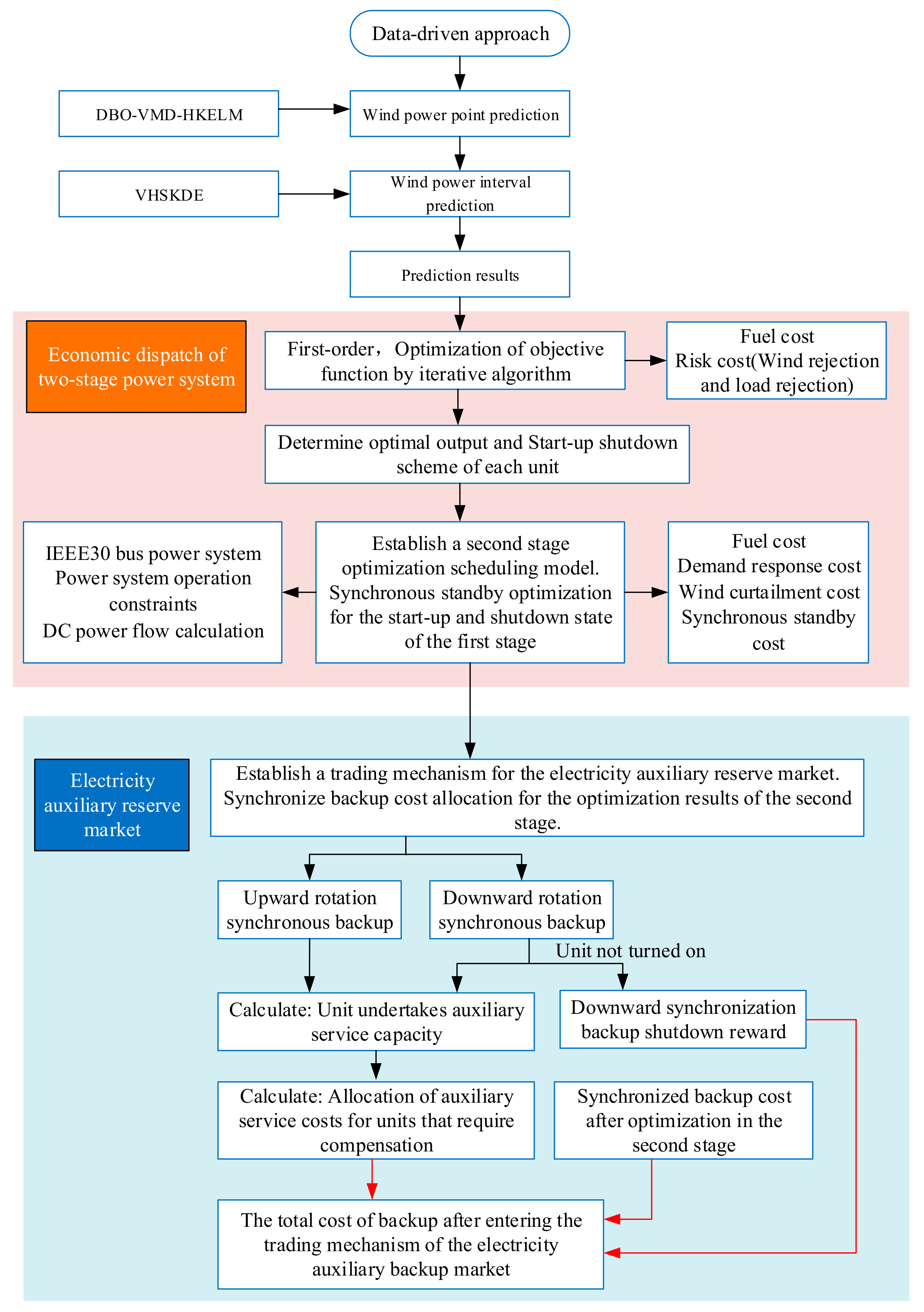
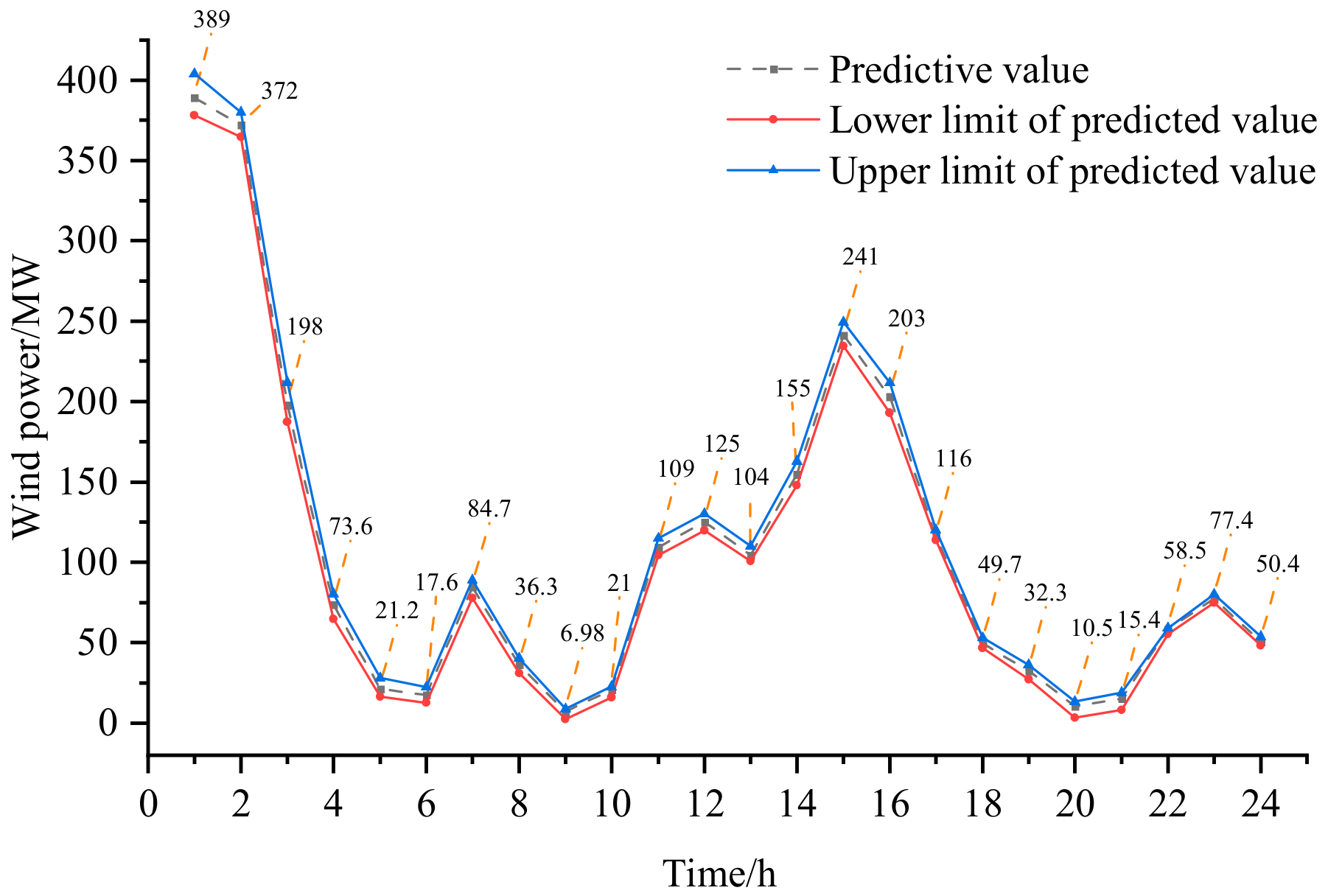
2.1.1. Data-Driven Wind Power Uncertainty Prediction

The uncertainty analysis relies on probabilistic interval forecasts of wind power. This analysis integrates an optimized machine learning wind power point prediction method with a hybrid kernel density estimation interval prediction method that accounts for ramp events. The data are from the actual operation data of a coastal wind farm in Northeast China in January 2022. A 120 m meteorological tower is installed in the wind farm to monitor meteorological data. The SCADA system collects the status information of each wind turbine at 1 min intervals. As the SCADA data from wind farms often contain numerous outliers, the variance change point percentile method is employed to clean and filter 44,640 data points of anomalies collected from each turbine in January. Missing data for each turbine are then interpolated using the nearest neighbor rule. Even the wind energy grid-connected new power system requires a forecast time resolution of 15 min for intraday scheduling. The sum of the active power for each turbine is averaged after processing to create 2976 wind power time series with a 15 min time resolution.

The paper introduces a novel wind power point forecasting model (DBO-VMD-HKELM). The model optimizes variational mode decomposition (VMD) parameters through the dung beetle optimizer (DBO) and employs the hybrid kernel extreme learning machine (HKELM). Considering the distribution characteristics of wind power prediction errors, the paper proposes an optimized interval assessment method (VHSKDE, Variable Bandwidth Hybrid Sliding Kernel Density Estimation) for wind power probability prediction. The term “Variable Bandwidth Hybrid” involves obtaining the probability density function of forecast deviations based on variable bandwidth kernel density estimations. This function is then weighted and superimposed according to the appropriate weighting coefficients, determined using the entropy weight method. The probability density functions obtained based on variable bandwidths exhibit different biases, and the bias superimposition mechanism compensates for each other. This enables the combined probability density function to more accurately estimate probability forecast deviations. Using the above method, the prediction results for 30 January are shown in Figure 2.

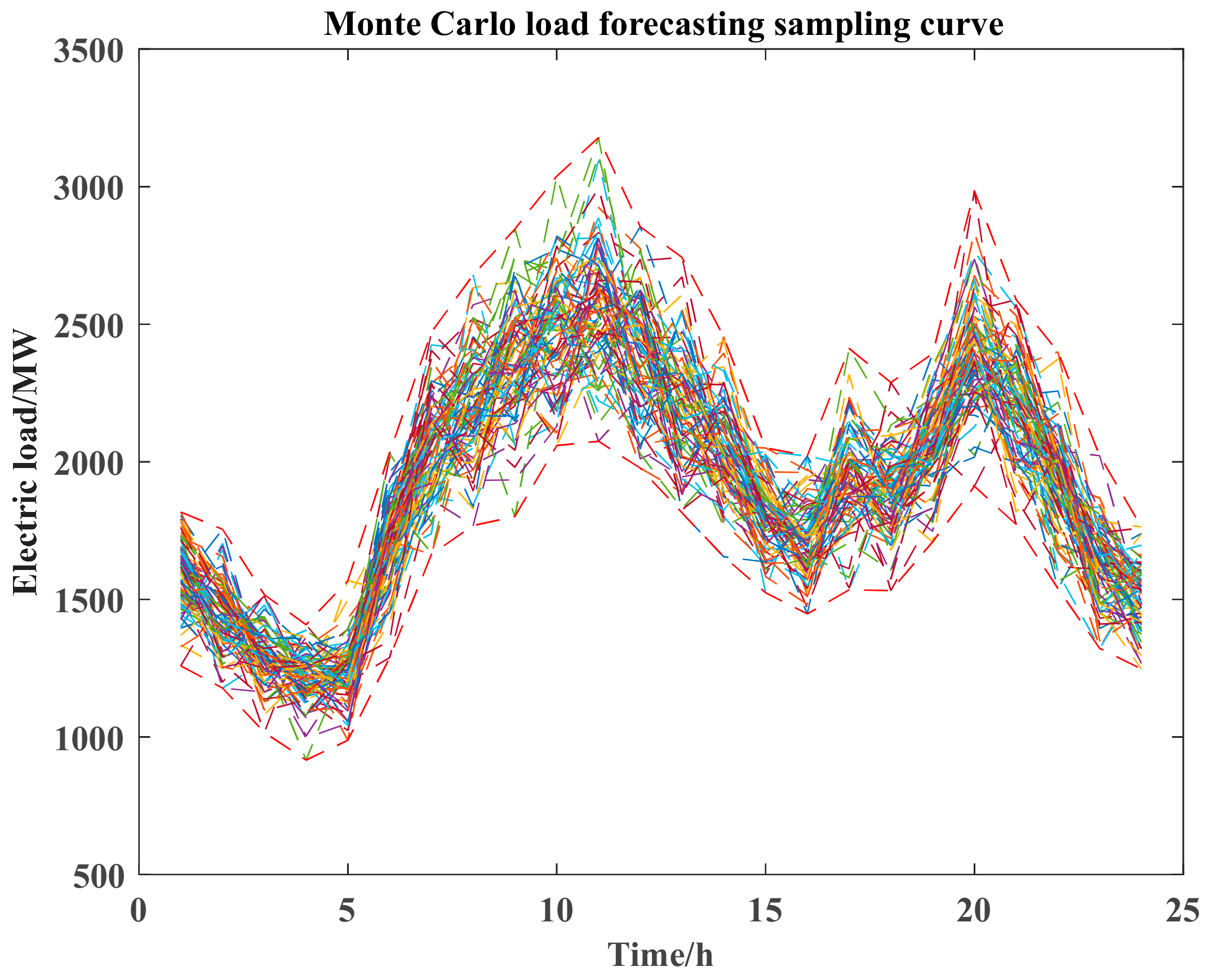
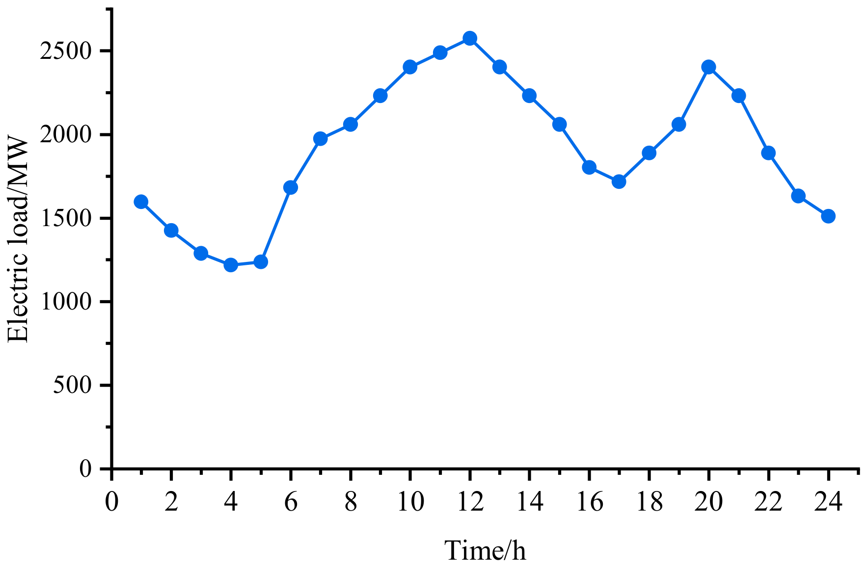
2.1.2. Load Uncertainty

The prediction error for the load is expressed as follows [22]:

$${\epsilon }_{l,n,t}=P_{l-true,n,t}-P_{l-pre,n,t}$$

(1)

where ${\epsilon }_{l,n,t}$, $P_{l-true,n,t}$, and $P_{l-pre,n,t}$ represent the prediction error, actual power, and predicted power of node load n at time period t, respectively. Short-term load prediction errors typically adhere to a normal distribution with an average value of 0, where the standard deviation ${\sigma }_{n,t}$ is determined based on the load prediction values coefficient q, as in Formula (2).

$${\sigma }_{n,t}=q{P}_{l-pre,n,t}$$

(2)

2.2. Risk Assessment Based on CVaR

To reduce the risk caused by wind power prediction deviations, conditional values at risk (CVaR) is employed to assess the losses associated with wind curtailment and load shedding. This assessment takes into account the volatility of wind power output, which can lead to the risk of load shedding and wind curtailment losses. The total prediction deviation be denoted as $\Delta f_{cva,t}$, where [23]

$$\Delta f_{cva,t}=\Delta f_{w,t}-\Delta f_{l,t}$$

(3)

$\Delta f_{l,t}$ stands for the prediction deviation of the load at time t, and $\Delta f_{w,t}$ stands for the prediction deviation of the wind power output at time t.

When the total prediction deviation is $\Delta f_{cva,t}<0$, indicating an excess demand for electric load, if the upward synchronous reserve capacity in the system cannot fully compensate for this, this results in a load shedding risk. Similarly, when the total prediction deviation is $\Delta f_{cva,t}>0$, indicating excess output power, insufficient downward synchronous reserve at this time leads to wind curtailment risk.

The calculation of load shedding (denoted as $f_{l,t}^{Reject}$) and wind curtailment (denoted as $f_{w,t}^{Reject}$) at time t is as shown in Formulas (4) and (5), respectively.

$$\begin{array}{cc}{f}_{l,t}^{Reject}=-\Delta f_{cva,t}-S_{u,t}& -\Delta f_{cva,t}>S_{u,t}\end{array}$$

(4)

$$\begin{array}{cc}{f}_{w,t}^{Reject}=\Delta f_{eva,t}-S_{d,t}& \Delta f_{eva,t}>S_{d,t}\end{array}$$

(5)

In the equations, $S_{u,t}$ stands for the upward synchronous reserve provided by the system at time t. $S_{d,t}$ stands for the downward synchronous reserve provided by the system at time t.

To evaluate the costs associated with the two risks mentioned above, the calculation methods are shown in Formulas (6) and (7).

$$\begin{array}{cc}{G}_{w,t}^W={\gamma }_w{f}_{w,t}^{Reject}& f_{w,t}^{Reject}\ge 0\end{array}$$

(6)

$$\begin{array}{cc}{G}_{l,t}^L={\gamma }_l{f}_{l,t}^{Reject}& f_{l,t}^{Reject}\ge 0\end{array}$$

(7)

In these equations, $G_{w,t}^W$ stands for the wind curtailment risk cost; ${\gamma }_w$ stands for the wind curtailment penalty cost coefficient; $G_{l,t}^L$ stands for the load shedding risk cost; and ${\gamma }_l$ stands for the load shedding penalty cost coefficient.

Thus, the CvaR values obtained from the uncertainty of wind power and load can be accurately assessed as follows [23]:

$$G_{CVaR}={\displaystyle \sum _{t=1}^T{G}_{w,t}^W+}{\displaystyle \sum _{t=1}^T{G}_{l,t}^L}$$

(8)

where the scheduling period is denoted by T.

2.3. Two-Stage Optimization Scheduling Model for Day Ahead

Considering the uncertainty of both generation and load, the system aims to minimize operating costs. To achieve this, two-stage optimization scheduling models are established which accord with the operational constraints of the new power system. These models incorporate fuel costs, various risk costs, wind curtailment costs, start-up and shutdown costs, as well as demand response costs.

2.3.1. Objective Function of the Two-Stage Optimization Model

In view of the uncertain predictions of wind power and load, the first-stage objective function is formulated, consisting of fuel costs for thermal power units and system risk costs. Optimization techniques are applied to solve this function, obtaining the optimal output of each unit and the optimal start-up and shutdown plans.

$$\min F_1=F_{11}+G_{CVaR}$$

(9)

$$F_{11}={\displaystyle \sum _{t=1}^T{\displaystyle \sum _{i=1}^N{\alpha }_i}}{P}_{i,t}^2+{\beta }_i{P}_{i,t}+{\lambda }_i$$

(10)

$$F_{Sp}=F_{Start}+F_{Stop}$$

(11)

$$\begin{array}{cc}{F}_{Start}={\displaystyle \sum _{i=1}^N{\displaystyle \sum _{t=1}^T{H}_i}}\cdot u_{i,t}& F_{Stop}={\displaystyle \sum _{i=1}^N{\displaystyle \sum _{t=1}^T{J}_i}}\cdot {\overline{u}}_{i,t}\end{array}$$

(12)

In the equation, $F_{11}$ stands for the fuel cost of thermal power units; $P_{i,t}$ stands for the planned output of thermal power unit i at time period t, where N is the total number of thermal power units; and ${\alpha }_i$, ${\beta }_i$, and ${\lambda }_i$ represent the generation cost coefficients of thermal power unit i. $F_{Sp}$ stands for the start-up and shutdown costs of thermal power units; $F_{Start}$ stands for the start-up cost; $F_{Stop}$ stands for the shutdown cost; and $H_i$ stands for the one-time start-up cost of thermal power unit i. $J_i$ stands for the one-time shutdown cost of thermal power unit i. $u_{i,t}$ stands for the start-up action variable at time period t. ${\overline{u}}_{i,t}$ stands for the shutdown action variable at time period t.

To establish the second-stage optimization scheduling model, synchronous reserve optimization is conducted while ensuring optimal economic dispatch conditions for the first-stage start-up and shutdown statuses. The objective function is formulated as follows:

$$\min F_2=F_{11}+F_{Cdr}+F_{Rw}+F_{Rec}$$

(13)

$$\begin{array}{cc}{F}_{Cdr}={\displaystyle \sum _{t=1}^T{\delta }_t{L}_{dr,t}}& F_{Rw}={\displaystyle \sum _{t=1}^T{\xi }_t(P_{w,t}-P_{wa,t})}\end{array}$$

(14)

$$F_{Rec}={\displaystyle \sum _{i=1}^N{\displaystyle \sum _{t=1}^T{\varsigma }_i^{up}{R}_{i,t}^{up}}}+{\varsigma }_i^{dw}{R}_{i,t}^{dw}$$

(15)

In the equation, $F_{Cdr}$ stands for the reducible load cost; ${\delta }_t$ stands for the reducible load cost coefficient at time period t; $L_{dr,t}$ stands for the reducible load at time period t. $F_{Rw}$ stands for the wind curtailment cost; and ${\xi }_t$ stands for the wind curtailment cost coefficient at time period t. $P_{wa,t}$ stands for the planned wind power output at time period t; $P_{w,t}$ stands for the predicted wind power output at time period t; $F_{Rec}$ stands for the standby cost of thermal power units; and ${\varsigma }_i^{up}$ and ${\varsigma }_i^{dw}$ respectively represent the price coefficients for providing the upward and downward reserve capacity of thermal power unit i. $R_{i,t}^{up}$ and $R_{i,t}^{dw}$ respectively represent the upward and downward reserve capacity provided by thermal power unit i at time period t.

2.3.2. Constraint Conditions

(1)

Constraint on the Start-Up and Shutdown of Thermal Power Units [22]

$$\begin{array}{cc}{\displaystyle \sum _{t=1}^{B_i}(1-u_{i,t})}=0& B_i\end{array}=\min \left\{T,(T_{u,i}-U_{i,0})u_{i,0}\right\}$$

(16)

$$\begin{array}{l}{\displaystyle \sum _{n=t}^{t+T_{u,i}-1}{u}_{i,n}}-T_{u,i}(u_{i,t}-u_{i,(t-1)})\ge 0\\ t=H_i+1,H_i+2,\cdots ,T-T_{u,i}+1\end{array}$$

(17)

$$\begin{array}{l}{\displaystyle \sum _{n=t}^T[u_{i,n}-(u_{i,t}-u_{i,(t-1)})]}\ge 0\\ t=T-T_{u,i}+2,T-T_{u,i}+3,\cdots ,T\end{array}$$

(18)

$$\begin{array}{cc}{\displaystyle \sum _{t=1}^{L_i}{u}_{i,t}}=0& L_i\end{array}=\min \left\{T,(T_{d,i}-S_{i,0})(1-u_{i,0})\right\}$$

(19)

$$\begin{array}{l}{\displaystyle \sum _{n=t}^{t+T_{d,i}-1}(1-u_{i,n})}-T_{d,i}(u_{i,(t-1)}-u_{i,t})\ge 0\\ t=L_i+1,L_i+2,\cdots ,T-T_{d,i}+1\end{array}$$

(20)

$$\begin{array}{l}{\displaystyle \sum _{n=t}^T[(1-u_{i,n})-(u_{i,(t-1)}-u_{i,t})]}\ge 0\\ t=T-T_{d,i}+2,T-T_{d,i}+3,\cdots ,T\end{array}$$

(21)

$$y_{i,t}-z_{i,t}=u_{i,t}-u_{i,t-1}$$

(22)

$$y_{i,t}+z_{i,t}\le 1$$

(23)

In the equations, $u_{i,t}$ stands for the operational state of thermal power unit i at time period t (0 denotes shutdown, 1 denotes operation); $T_{d,i}$ and $T_{u,i}$ respectively represent the minimum shutdown and minimum operation time of thermal power unit i; $U_{i,0}$ and $S_{i,0}$ respectively represent the initial start-up and shutdown operation time of thermal power unit i; and $y_{i,t}$ and $z_{i,t}$ respectively represent the start-up and shutdown variables of general unit i at time period t.

(2)

Constraint on the Ramping of Thermal Power Units [22]

$$(P_{i,t}+R_{i,t}^{up})-(P_{i,t-1}-R_{i,t-1}^{dw})\le r_{up,i}\Delta T(1-y_{i,t})+P_{i,\min }{y}_{i,t}$$

(24)

$$(P_{i,t-1}+R_{i,t-1}^{up})-(P_{i,t}-R_{i,t}^{dw})\le r_{dw,t}\Delta T(1-z_{i,t})+P_{i,\min }{z}_{i,t}$$

(25)

where $r_{up,i}$ and $r_{dw,i}$ respectively represent the upward and downward ramping rates of thermal power units, and $\Delta T$ stands for the scheduling time interval.

(3)

Constraint on the Output Limits of Thermal Power Units

$$P_{i,t}+R_{i,t}^{up}\le P_{i,\max }{u}_{i,t}$$

(26)

$$P_{i,t}-R_{i,t}^{dw}\ge P_{i,\min }{u}_{i,t}$$

(27)

In the equations, $P_{i,\max }$ and $P_{i,\min }$ respectively represent the upper and lower limits of the output of thermal power unit i.

(4)

Wind Power Output Constraint

$$0\le P_{wa,t}\le P_{w,t}$$

(28)

(5)

Load Balance Constraint

$${\displaystyle \sum _{i=1}^{N_h}{P}_{i,t}}+{\displaystyle \sum _{w=1}^{N_w}{P}_{wa.t}}-{\displaystyle \sum _{n=1}^{N_N}{L}_{dr,t}}={\displaystyle \sum _{n=1}^{N_N}{L}_{l,t}}$$

(29)

where $L_{l,t}$ stands for the node load at time period t, $N_N$ stands for the number of nodes in the new power system, $N_h$ stands for the number of thermal power units, and $N_w$ stands for the number of wind farms.

(6)

Synchronous Reserve Constraint

$$\begin{array}{l}0\le U_{i,t}\le u_{i,t}\cdot \theta \cdot P_{i,\max }\\ 0\le D_{i,t}\le u_{i,t}\cdot \theta \cdot P_{i,\max }\end{array}$$

(30)

$$\begin{array}{cc}{U}_{i,t}\le P_{i,\max }-P_{i,t}& D_{i,t}\le P_{i,t}-P_{i,\min }\end{array}$$

(31)

$$\begin{array}{l}{\displaystyle \sum _{i=1}^{N_h}{U}_{i,t}\ge }{\nu }_w{\displaystyle \sum _{w=1}^{N_w}{P}_{wa.t}}+{\nu }_l\cdot {\displaystyle \sum _{n=1}^{N_N}{L}_{l,t}}\\ {\displaystyle \sum _{i=1}^{N_h}{D}_{i,t}\ge }{\mu }_w{\displaystyle \sum _{w=1}^{N_w}{P}_{wa.t}}+{\mu }_l\cdot {\displaystyle \sum _{n=1}^{N_N}{L}_{l,t}}\end{array}$$

(32)

where $U_{i,t}$ and $D_{i,t}$ respectively represent the upward and downward synchronous reserve of thermal power unit i at time period t; $\theta$ stands for the reserve coordination coefficient; $P_{i,\min }$ stands for the minimum output of thermal power units; ${\nu }_w$ and ${\nu }_l$ respectively represent the positive thermal reserve fluctuation coefficients of wind farms and loads; and ${\mu }_w$ and ${\mu }_l$ respectively represent the negative thermal reserve fluctuation coefficients of wind farms and loads.

(7)

Line Flow Constraint [23]

$${\displaystyle \sum _{i=1}^{N_h}{K}_{l,i}}{P}_{i,t}+{\displaystyle \sum _{w=1}^{N_w}{K}_{l.w}}{P}_{wa.t}-{\displaystyle \sum _{n=1}^{N_N}{K}_{l,n}{P}_{n,t}}\le P_{l,\max }$$

(33)

$$-({\displaystyle \sum _{i=1}^{N_h}{K}_{l,i}}{P}_{i,t}+{\displaystyle \sum _{w=1}^{N_w}{K}_{l,w}{P}_{wa,t}}-{\displaystyle \sum _{n=1}^{N_N}{K}_{l,n}}{P}_{n,t})\le P_{l,\max }$$

(34)

In the equations, $K_{l,i}$, $K_{l.w}$, and $K_{l,n}$ respectively represent the power injection transfer distribution factors from thermal power unit i, wind farm w, and load n to transmission line l. $P_{l,\max }$ stands for the maximum transmission capacity of line l. Equations (28) and (29) respectively represent the limit constraints for forward and reverse power flows on the transmission line.

2.3.3. Improved Binary Fish Swarm Optimization Algorithm

The fish swarm algorithm (FSA) [24] is an evolutionary algorithm based on simulating the behavior of fish swarms. It mimics the behaviors of fish in foraging and avoiding predators, and it is applied to solve optimization problems. Using a bottom-up optimization strategy, the FSA achieves global optimization through the local optimization of individuals within the fish swarm, demonstrating features such as parallelism, simplicity, globality, speed, and tracking ability. Assuming the search space dimensionality is D, each particle’s information is represented by two D-dimensional vectors: the fish’s position $X_i=(x_{i,1},x_{i2},\cdots ,x_{iD})$ and velocity vector $V_i=(v_{i1},v_{i2},\cdots ,v_{iD})$. Each fish has an adaptation value determined by the optimal objective function used to evaluate the quality of the fish’s current position. During the iterative process of the algorithm, fish continuously adjust their positions and velocities by learning from both the “individual perception of food concentration” and the “population perception of food concentration”, rapidly and accurately approaching the target. Here, the “individual perception of food concentration” refers to the individual extreme values point found by each fish in the search space, denoted as P. The “Population perception of food concentration” refers to the global extreme values point found by the entire fish swarm in the search space, denoted as G. The updated formulas for the fish swarm’s position and velocity information are as follows:

$$x_{id}^{j+1}=x_{id}^j+v_{id}^{j+1}$$

(35)

$$v_{id}^{j+1}=\omega v_{id}^j+c_1{r}_1(P_{id}^j-x_{id}^j)+c_2{r}_2(G_d^j-x_{id}^j)$$

(36)

In the equations, $\omega$ stands for the inertia weight; $r_1$ and $r_2$ are random numbers in the range [0, 1]; $c_1$ and $c_2$ are learning factors, typically in the range of [0, 2]; and $x_{id}^j$ and $v_{id}^j$ represent the position and velocity of fish i at the d-th position in the j-th iteration. $P_{id}^j$ stands for the values of the individual extreme values point of fish i at the d-th position in the j-th iteration, and $G_d^j$ stands for the values of the global extreme values point of the fish swarm at the d-th position in the j-th iteration. The unit start–stop is a 0–1 nonlinear integer optimization problem, requiring an improvement of the traditional fish swarm algorithm used for solving continuous variable optimization problems. This improvement involves using the double-layer binary fish swarm optimization (DLBFSO) algorithm for solving.

In the DLBFSO algorithm, each bit of the fish position vector takes a value of 0 or 1. The algorithm calculates the probability of each position taking the value of 0 or 1 using a Sigmoid function with velocity as a variable. The updated formulas for the fish position and velocity information are as follows:

$$Sigmoid(v_{id}^{j+1})=\frac{1}{1+e^{-v_{id}^{j+1}}}$$

(37)

$$x_{id}^{j+1}=\left\{\begin{array}{l}\begin{array}{cc}1& rand<Sigmoid(v_{id}^{j+1})\end{array}\\ \begin{array}{cc}0& rand\ge Sigmoid(v_{id}^{j+1})\end{array}\end{array}\right.$$

(38)

In the equations, “rand” stands for a number in the range [0, 1].

The double-layer fish swarm algorithm comprises two levels of fish swarm updates: global layer update and local layer update.

Global layer update: this guides the movement of the fish swarm based on the global optimum solution (global optimal fish swarm) to accelerate the global search.

Local layer update: this directs the movement of particles based on the local optimum solution (local optimal fish swarm) to expedite the local search.

2.3.4. Seagull Optimization Algorithm (SOA)

Gulls, as flocking organisms, exhibit two important behavioral traits: migration and aggression. During group migration, to avoid collisions, gulls update their initial position by moving in a direction that is more suitable for survival. In the process of catching food at sea, the gulls attack the prey by moving in a spiral pattern, taking the prey’s location as the optimal position and obtaining the optimal fitness value [25].

(1)

Migration of seagulls (global search)

The gull migration process simulates the movement behavior of a gull colony from one location to another. Three conditions should be satisfied in this global search phase. Condition 1: avoid collision; Condition 2: the determination of the optimal positional orientation; and Condition 3: move to the optimal position.

(2)

Seagull attack (localized search)

The gulls use their wings to change their angle of attack and speed when hunting during migration, attacking their prey in a spiral motion in the a, b, and c planes, thus updating the gull’s position.

$$P_s(x)=abc{d}_s(x)+P_b(x)$$

(39)

$$\left\{\begin{array}{c}r=u\times e^{\beta \nu }\\ a=r\times \cos (\beta )\\ b=r\times \sin (\beta )\\ c=r\times \beta \end{array}\right.$$

(40)

where $P_s(x)$ stands for updated location after a seagull attack; $r$ stands for the radius of each circle of the helix; $u$ and $\nu$ are constants that define the shape of the helix; e is the base of the natural logarithm; and $\beta$ is a number in the range of $[0,2\pi ]$.

2.4. Assessment Mechanism for Power Auxiliary Reserve Market

Regarding the upward synchronous reserve, the first step is to calculate the capacity values of each unit providing ancillary services.

When the unit is not operating, the upward synchronous reserve is required, and the capacity needs to be allocated based on the maximum technical output values. The formula is as follows:

$$\left\{\begin{array}{l}\begin{array}{cc}{J}_{i,t}=P_{\max ,i},& P_{i,t}=0\end{array}\\ \begin{array}{cc}{J}_{i,t}=P_{i,t},& P_{i,t}\ne 0\end{array}\end{array}\right.$$

(41)

where $J_{i,t}$ stands for the allocated capacity of each unit for the upward synchronous reserve.

According to the proportion of unit capacity, the obligation is determined, and the responsibility of each unit is calculated. The formula is as follows:

$$\begin{array}{cc}{M}_t={\displaystyle \sum _{i=1}^{N_h}{J}_{i,t}}& URe{f}_{i,t}=\frac{J_{i,t}}{M_t}\end{array}$$

(42)

$$Refu{p}_{i,t}=URe{f}_{i,t}\cdot J_{i,t}$$

(43)

where $M_t$ stands for the total output capacity of each unit for the upward synchronous reserve in time period t, $URe{f}_{i,t}$ stands for the proportion of the upward synchronous reserve capacity for each unit in time period t, and $Refu{p}_{i,t}$ stands for the capacity of the upward synchronous reserve that each unit undertakes based on the proportion of $URe{f}_{i,t}$.

The formula for determining the penalized capacity of units requiring upward synchronous reserve compensation is as follows:

$$\Delta U_{i,t}=U_{i,t}-Refu{p}_{i,t}$$

(44)

$$\left\{\begin{array}{l}\begin{array}{cc}\Delta U_{i,t}=0,& \Delta U_{i,t}>0\end{array}\\ \begin{array}{cc}\Delta U_{i,t}=\left|\Delta U_{i,t}\right|,& \Delta U_{i,t}\le 0\end{array}\end{array}\right.$$

(45)

where $U_{i,t}$ stands for the upward synchronous reserve capacity, and $\Delta U_{i,t}$ stands for the penalized capacity for the upward synchronous reserve.

To allocate the ancillary service cost among units based on the difference in the upward synchronous reserve penalized capacity, the formula is as follows:

$${\psi }_{i,t}=\frac{\Delta U_{i,t}}{{\displaystyle \sum _{i=1}^{N_h}\Delta U_{i,t}}}\cdot ({\displaystyle \sum _{i=1}^{N_h}{f}_{up,i,t}\cdot U_{i,t}})$$

(46)

where ${\psi }_{i,t}$ stands for the allocated penalized cost of ancillary service for the upward synchronous reserve among units, and $f_{up,i,t}$ stands for the upward synchronous reserve cost coefficient.

The total cost calculation for the penalized upward synchronous reserve among units is as follows:

$$R_{upcf}={\displaystyle \sum _{t=1}^T{\displaystyle \sum _{i=1}^{N_h}{\psi }_{i,t}}}$$

(47)

For the downward synchronous reserve, the calculation of the capacity each unit needs to bear is based on the minimum technical output of each unit:

$$DRe{f}_{i,t}=\frac{P_{i,t}-P_{i,\min }}{{\displaystyle \sum _{i=1}^{N_h}{P}_{i,t}}}$$

(48)

$$\left\{\begin{array}{l}\begin{array}{cc}DRe{f}_{i,t}=0,& DRe{f}_{i,t}<0\end{array}\\ \begin{array}{cc}DRe{f}_{i,t}=DRe{f}_{i,t},& DRe{f}_{i,t}\ge 0\end{array}\end{array}\right.$$

(49)

$$Refdow{n}_{i,t}=DRe{f}_{i,t}\cdot P_{i,t}$$

(50)

where $DRe{f}_{i,t}$ stands for the proportion of capacity each unit needs to bear for the downward synchronous reserve based on the minimum technical output, and $Refdow{n}_{i,t}$ stands for the capacity each unit needs to bear for downward synchronous reserve.

The formula for determining the penalized capacity of units requiring downward synchronous reserve compensation is as follows:

$$\Delta D_{i,t}=D_{i,t}-Refdow{n}_{i,t}$$

(51)

$$\left\{\begin{array}{l}\begin{array}{cc}\Delta D_{i,t}=0,& \Delta D_{i,t}>0\end{array}\\ \begin{array}{cc}\Delta D_{i,t}=\left|\Delta D_{i,t}\right|,& \Delta D_{i,t}\le 0\end{array}\end{array}\right.$$

(52)

where $D_{i,t}$ stands for the downward synchronous reserve capacity, and $\Delta D_{i,t}$ stands for the penalized capacity for the downward synchronous reserve.

To allocate the ancillary service cost among units based on the difference in penalized capacity for the downward synchronous reserve, the formula is as follows:

$$\left\{\begin{array}{l}\begin{array}{cc}{\overline{\psi }}_{i,t}=\frac{\Delta D_{i,t}}{{\displaystyle \sum _{i=1}^{N_h}\Delta D_{i,t}}}\cdot {\displaystyle \sum _{i=1}^{N_h}{f}_{down,i,t}\cdot D_{i,t}}& \Delta D_{i,t}>0\end{array}\\ \begin{array}{cc}{\overline{\psi }}_{i,t}=0& \Delta D_{i,t}=0\end{array}\end{array}\right.$$

(53)

where $f_{down,i,t}$ stands for the downward synchronous reserve cost coefficient, and ${\overline{\psi }}_{i,t}$ stands for the allocated penalized cost of ancillary service for the downward synchronous reserve among units.

The total cost calculation for the penalized downward synchronous reserve among units is as follows:

$$R_{downcf}={\displaystyle \sum _{t=1}^T{\displaystyle \sum _{i=1}^{N_h}{\overline{\psi }}_{i,t}}}$$

(54)

In relation to the mechanism for downward synchronous reserve rewards, the calculation of the capacity each unit needs to bear for ancillary service rewards must be carried out. This refers to determining the capacity reward for units in shutdown status. To optimize the system’s reserve plan and reduce the cost of the downward synchronous reserve, this paper sets the maximum technical output values of the unit as the reward capacity as follows:

$$\left\{\begin{array}{l}\begin{array}{cc}{K}_{i,t}=P_{\max ,i},& P_{i,t}=0\end{array}\\ \begin{array}{cc}{K}_{i,t}=0& P_{i,t}\ne 0\end{array}\end{array}\right.$$

(55)

where $K_{i,t}$ stands for the allocated reward capacity of each unit for the downward synchronous reserve.

Following the reward capacity for units in shutdown status for the downward synchronous reserve, the formula for the sharing of ancillary service rewards among units is as follows:

$$Q_{i,t}=K_{i,t}\cdot \frac{({\displaystyle \sum _{i=1}^{N_h}{f}_{down,i,t}\cdot D_{i,t}})}{{\displaystyle \sum _{i=1}^{N_h}{D}_{i,t}}}$$

(56)

where $K_{i,t}$ stands for the allocated reward capacity of each unit for the downward synchronous reserve, and $Q_{i,t}$ stands for the sharing of rewards among units for the downward synchronous reserve.

The calculation of the total rewards of ancillary service for the downward synchronous reserve among units is as follows:

$$R_{downjl}={\displaystyle \sum _{t=1}^T{\displaystyle \sum _{i=1}^{N_h}{Q}_{i,t}}}$$

(57)

3. Example Analysis

The IEEE 30-node system serves as a case study to validate the availability and feasibility of the proposed two-stage scheduling model and evaluation model of the standby ancillary service market. The optimization software CPLEX (12.10.0) is invoked using the Yalmip toolbox on the Matlab (R2023a) platform for model solving. The configuration includes an Intel Core I9-13900HX series processor with a frequency of 2.2 GHz and 16 GB of memory.

3.1. IEEE 30 Node System Example

The improved IEEE 30-node system comprises 11 thermal power units, one wind farm, and 41 transmission lines [26]. The connection nodes of each unit are detailed in

Table 1. Statistics of access nodes of each unit.

Node Number	Maximum Output/MW	Minimum Output /MW	Climbing Rate	Start-Up Cost/USD	Downtime Costs/USD
1	100	20	25	6	2
2	200	50	50	7	3
6	100	20	25	6	2
7	500	100	125	12	4
8	100	20	25	6	2
9	300	100	75	8	4
10	300	100	75	8	4
14	100	30	25	6	2
17	500	300	125	12	4
19	500	300	125	12	4
21	100	10	25	6	2

. Wind power operation data are sourced from a wind farm in a coastal area in Northeast China, with the connection node identified as node 12. The transmission capacity limit for all lines is set at 250 MW. Figure 3 depicts the Monte Carlo simulation of the load curve, vividly showcasing the uncertainty of the load [27]. From Figure 3, one scenario is selected to represent the system’s total load prediction curve, as illustrated in Figure 4.

In order to verify the effectiveness of the two-stage optimal scheduling method considering CVaR and synchronous reserve, and ensure the effective allocation of reserve, four scenarios are established to verify the economy of the reserve auxiliary service market evaluation model. Four system operation scenarios are developed for comparative analysis, as shown in

Table 2. Comparison analysis of system operation schemes.

Scheme	Phase 1	Phase 2
Scenario 1	Start–stop optimization without considering operational risks	Disregard synchronous spare optimization
Scenario 2	Start–stop optimization without considering operational risks	Consider synchronous spare optimization
Scenario 3	Consider start–stop optimization of operating risks	Disregard synchronous spare optimization
Scenario 4	Consider start–stop optimization of operating risks	Consider synchronous spare optimization

.

To explore the volatility of wind power on the supply side and the robustness of the established optimization models, this study utilizes data-driven wind power uncertainty prediction results for validation. Three circumstances are considered: the upper limits of wind power forecast values (Circumstance 1), the lower limits of wind power forecast values (Circumstance 2), and wind power forecast values (Circumstance 3).

3.2. Analysis of Reserve Limits for Wind Power Systems Based on Uncertainty

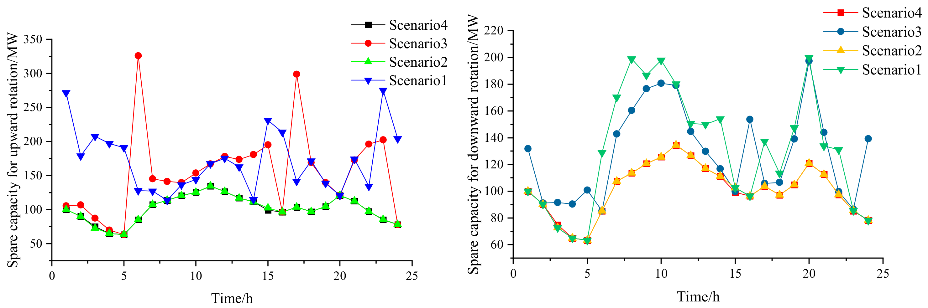
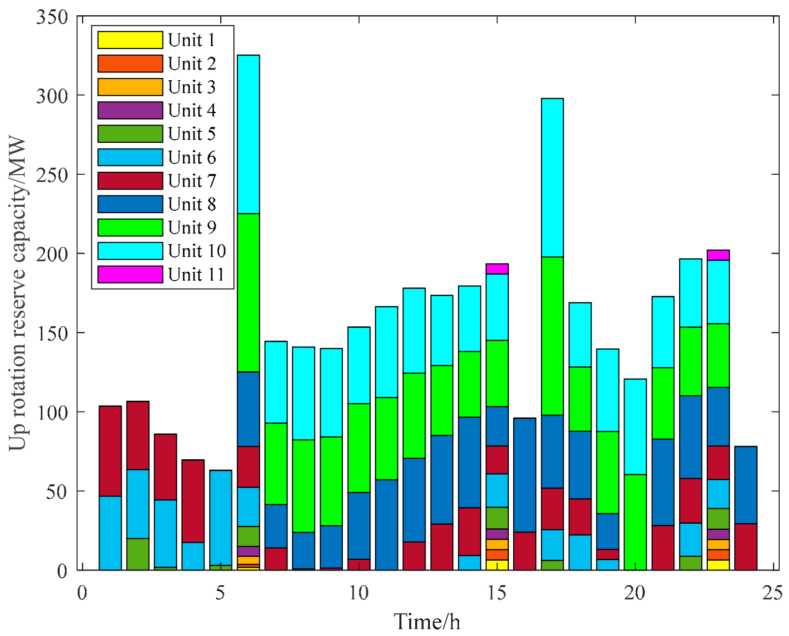
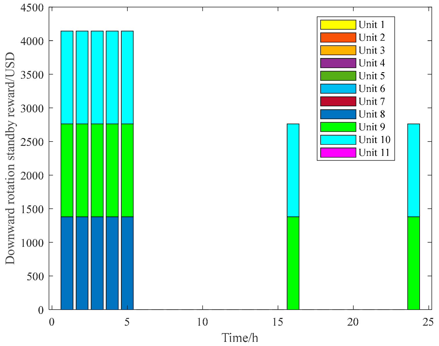
3.2.1. Analysis of the Effectiveness of the Evaluation Model of the Upper Limit Standby Auxiliary Service Market Based on Wind Power Forecasts

It is important to verify the robustness of the two-stage optimal dispatch methodology, taking into account the new power system operational risk and synchronized standby and its impact on the power auxiliary standby market assessment. The upper and lower extremes of the wind power interval forecasts are used to further validate the effectiveness and feasibility of the methodology in this paper.

The system operating costs of the four scenarios based on the upper limit of wind power values (Circumstance 1) are shown in

Table 3. System operating cost statistics for four scenarios in view of upper limit of wind power forecast.

Cost/USD	Scenario 1	Scenario 2	Scenario 3	Scenario 4
Fuel	156,600	156,723	150,482	150,736
Abandoned wind	4727	4727	7306	7306
Reducible load	3711	3711	4266	4266
Start-up and shutdown	2076	2076	1984	1984
Synchronized reserve	21,977	12,939	20,613	12,665
Operating before assessment	189,092	180,177	184,651	176,957

.

Considering Table 3 combined with Figure 5, the results of the analysis of operating cost and standby capacity are as follows: in the first stage of start–stop optimization without considering the operating risk, Scenario 2 is compared with Scenario 1, in which the fuel cost of Scenario 1 is lower than Scenario 2, the upward and downward synchronous standby capacity of Scenario 2 is lower than Scenario 1, and the synchronous standby cost of Scenario 1 is significantly higher than that of Scenario 2. In the first stage, when the start-up and shutdown of the operation risk are optimized by DLBFSO, the fuel cost of Scenario 4 is slightly higher than Scenario 3, and the synchronous standby cost of Scenario 4 is lower than that of Scenario 3. From the above results, it can be seen that in the second stage of the optimization without considering the synchronous standby, the system of Scenario 1 and Scenario 3 has too much synchronous standby reserved, which makes the solution too conservative, and the overall economy deteriorates. Scenarios 4 and 2 obtain the optimal configuration strategy by considering the optimization of synchronous standby costs and coordinating the system unit output with the synchronous standby capacity in a compromise. As a result, the total system operating costs before the new power system participation evaluation are reduced by USD 8915 and USD 7694, respectively.

Through the comparison of the above studies, the operating cost of the second stage considering synchronized standby optimization is optimal. Then, the operating cost comparison analysis is carried out through Scenario 4 and Scenario 2. Scenario 4, through the start–stop optimization model considering the operating risk in the first stage, optimally configures the start–stop state and the optimal output of each unit, which results in the optimal operating cost of the system’s thermal power units. Due to the increase in wind abandonment and curtailable load, the reserved synchronous standby capacity of the system is reduced, the pressure of synchronous standby cost is eased, and the cost of wind abandonment and curtailable load is increased. To cope with this problem, the second stage of the standby cost optimization model is adopted, which makes the wind power output, curtailable load, and synchronous standby capacity become reasonably and efficiently configured, and the operation results show that although the cost of wind abandonment and the cost of curtailable load are increased, the fuel cost is increased. The operating results show that although the wind abandonment cost and curtailable load cost are increased, the fuel cost, start–stop cost, and standby cost are reduced, and the total operating cost before evaluation is reduced by USD 3220. Therefore, through the optimization of the two stages and the effective coordination of the economy and operation risk, Scenario 4 is the optimal scheduling strategy.

Figure 6, Figure 7, Figure 8 and Figure 9 show the shared upward and downward synchronized standby capacity of each unit for Scenario 4 and Scenario 3, respectively. In Scenario 3, the up-synchronized standby capacity is mainly provided by the economic units 7, 8, 9, and 10, and the down-synchronized standby capacity is provided by units 5, 6, 7, and 8 to ensure economy. Scenario 4 considers the availability of standby cost on the basis of Scenario 3 and optimizes the size of standby capacity in each time period and the proportion of standby capacity distribution among units in the iterative solution process, with the optimized units 3, 7, and 8 providing the up-synchronous standby capacity and units 2, 3, 4, 7, and 8 providing the down-synchronous standby capacity. By considering the synchronized standby cost optimization, the economy of system operation is effectively coordinated.

In traditional methods, the incomplete settlement mechanism of the backup market has led to the additional cost of wind power and load, which has caused unnecessary efficiency and economic losses in the market. This article proposes a spare market reward and punishment mechanism, that is, the marketing principle of “who generates, who will bear”, that is, the force of each unit needed to distribute the backup cost and set the maximum technical contribution values of the crew as a reward to avoid the additional costs caused by the mismatch of the backup cost and rewarding the efficient guidance of various units and reasonable economic configurations.

Table 4. Operation results of clearing mechanism in standby market based on the upper limit of wind power forecast.

Cost/USD	Scenario 1	Scenario 2	Scenario 3	Scenario 4
Upward synchronization backup penalty	13,411	6893	12,012	6803
Downward synchronization backup penalty	5178	4979	7125	5863
Downward synchronization standby reward	8166	7396	26,256	22,846
Backup after assessment	32,310	17,415	13,494	2485
Operation after assessment	199,515	184,653	177,532	166,777

is the results of the reward and punishment mechanism of the spare service market.

Based on the four scheduling scenarios, the total cost of backup is evaluated on the basis of the previous backup cost, taking into account the up-synchronized backup penalty cost, down-synchronized backup penalty cost, and reward cost. For the up-synchronized standby, the standby capacity is shared according to the proportion of the standby capacity of each unit based on the output of each unit. Then, the up-synchronized standby penalty cost is obtained by apportioning the auxiliary service cost of each unit according to the difference in the up-synchronized standby. For the down-synchronized standby, the down-synchronized standby capacity is calculated based on the minimum technical output of each unit. Then, the downward synchronized standby penalty cost is obtained by apportioning the cost of auxiliary services of each unit according to the downward synchronized standby difference. For the synchronized standby reward, the maximum technical output of each unit is set as the reward capacity. Then, the downward synchronized standby reward cost is obtained by apportioning the auxiliary service reward of each unit according to the downward synchronized standby downtime reward capacity. Under the standby market assessment mechanism proposed in this paper, the two-stage optimization makes the post-assessment running cost and standby cost of traditional generating units lower and better utilizes the advantage of the marginal cost of new energy.

Table 4 analyzes the costs after the application of the proposed auxiliary standby market assessment model for settlement. The first-stage optimization model optimally allocates the start–stop states and optimal output of each unit, resulting in the optimal total cost of backup after evaluation. Scenarios 3 and 4 are significantly better than Scenarios 1 and 2, where the corresponding lower synchronized standby reward costs exceed USD 20,000 each. The second stage of synchronous standby optimization effectively coordinates the system unit output and synchronous standby capacity to obtain an optimal configuration strategy, and the results show that Scenario 4 is significantly better than Scenario 3, and Scenario 4 has a lower upper synchronous standby penalty cost and lower synchronous standby penalty cost, which reduces the evaluated total standby cost by USD 11,009 and also reduces the evaluated total operating cost by USD 10,755.

Figure 10, Figure 11, Figure 12 and Figure 13 show the results of the upper and lower synchronized standby penalty cost sharing by unit and by time period for Scenario 4 and Scenario 3. The upper standby penalty cost for Scenario 4 is below USD 400 for all time periods, while Scenario 3 is below USD 400 for only a few time periods. Similarly, the lower standby penalty cost for Scenario 4 is almost less than USD 300, while Scenario 3 has 11 periods that are significantly more than USD 300. Therefore, Scenario 4 can significantly save the upward and downward synchronized standby penalty cost, and the penalty cost shows that Scenario 4 makes the standby configuration of each time period relatively average, and the fluctuation amplitude is smoother, which is helpful for the timely adjustment and stable operation of the new power system standby.

Figure 14 and Figure 15 show the results of the shared reward cost by unit and time period for down-synchronized standby for Scenario 4 and Scenario 3. The down-synchronized standby outage reward benefits are better for Scenario 3 than for Scenario 4, with the rewards contributing primarily to units 8, 9, and 10 compared to Scenario 3.

Looking at the overall evaluation results, the reward benefits of Scenario 3 are not sufficient to cover its total up and down synchronization standby penalty costs. Scenario 4 has total post-evaluation standby cost savings of USD 11,009 compared to Scenario 3. The total post-evaluation operating cost savings is USD 10,755. Therefore, Scenario 4 and the proposed standby ancillary services market reward and penalty mechanism effectively guide the new energy sources to bear part of the standby costs and realize the reasonable sharing of energy and standby costs.

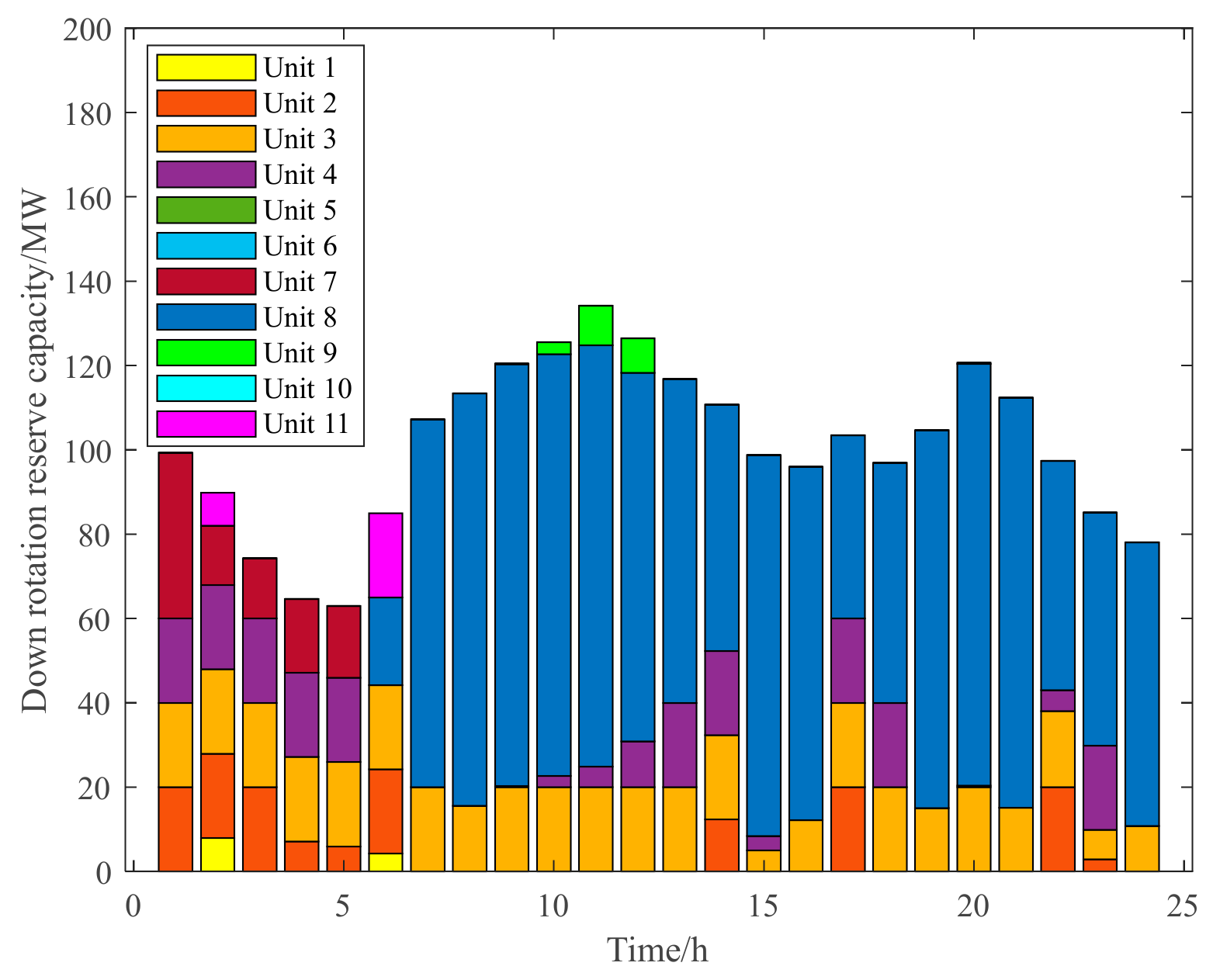
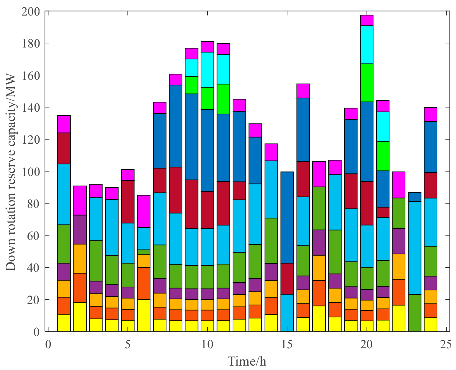
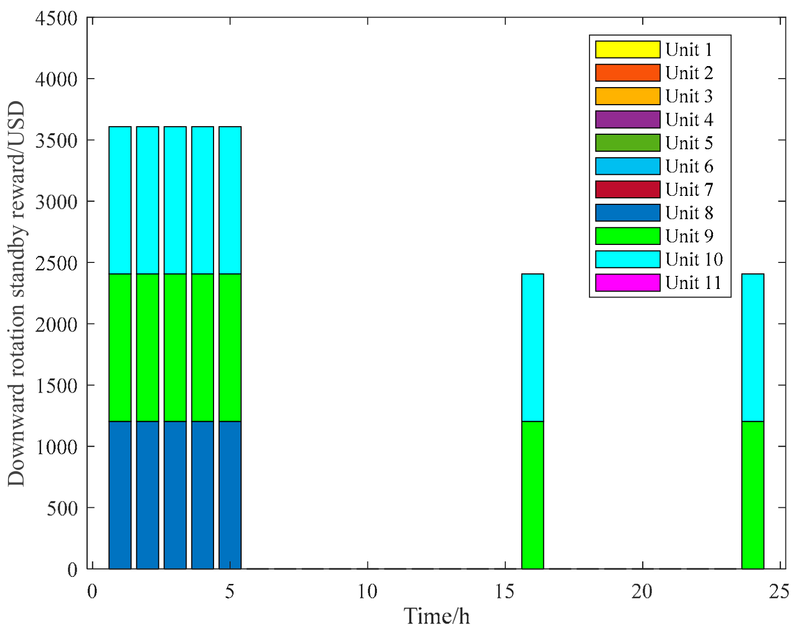
3.2.2. Analysis of the Effectiveness of the Evaluation Model of the Lower Limit Standby Auxiliary Service Market Based on Wind Power Forecasts

The system operating costs of the four scenarios based on the lower limit of the wind power forecasts (Circumstance 2) are shown in

Table 5. System operation costs of four schemes based on the lower limit of wind power forecast.

Cost/USD	Scenario 1	Scenario 2	Scenario 3	Scenario 4
Fuel	157,391	157,520	151,638	151,875
Abandoned wind	2233	2233	7552	7552
Reducible load	3818	3818	4264	4264
Start-up and shutdown	2076	2076	1984	1984
Synchronized reserve	21,841	12,875	20,538	12,596
Operating before assessment	187,359	178,522	185,976	178,271
Upward synchronization backup penalty	13,253	6863	11,927	6765
Downward synchronization backup penalty	5092	4955	7471	5831
Downward synchronization standby reward	8169.6	7391	26,219	22,849
Backup after assessment	32,016	17,302	13,716	2344
Operation after assessment	197,534	182,948	179,155	168,019

.

In the first stage of start–stop optimization without considering operational risk, Scenario 2 vs. Scenario 1, the optimization of standby costs results in a reduction in system standby costs by USD 8966. In the first stage with start–stop optimization considering operational risk, Scenario 4 compares with Scenario 3, and the optimization of standby cost results in a reduction in system standby cost by USD 7642, and in the second stage with simultaneous standby optimization scenarios considered, Scenario 4 compares with Scenario 2, and the total pre-assessment operational cost is reduced by USD 251. Therefore, in the case of the upper limit of the wind forecast as a baseline, Scenario 4 is able to achieve a reduction in system standby cost by considering the above-mentioned factors. Therefore, in the case of the upper limit of the wind power forecast, Scenario 4 achieves the efficient allocation of system standby resources and the optimal economic dispatch of the system by considering the two-phase optimization of start–stop, conditional risk, and synchronous standby.

Table 5 analyzes the costs after the application of the proposed auxiliary standby market assessment model for settlement. The first-stage optimization model optimally allocates the start–stop states and optimal output of each unit, resulting in the optimal total cost of backup after evaluation. Scenarios 3 and 4 are significantly better than Scenarios 1 and 2, where the corresponding lower synchronized standby reward costs exceed USD 20,000 each. The second stage of synchronous standby optimization effectively coordinates the system unit output and synchronous standby capacity to obtain an optimal configuration strategy, and the results show that Scheme 4 is significantly better than Scheme 3, and Scheme 4 has a lower upper synchronous standby penalty cost and lower synchronous standby penalty cost, which reduces the evaluated total standby cost by USD 11,372 and also reduces the evaluated total operating cost by USD 11,136.

Looking at the overall evaluation results, the reward benefits of Scenario 3 are not sufficient to cover its total up and down synchronization standby penalty costs. Scenario 4 has total post-evaluation standby cost savings of USD 11,372 compared to Scenario 3. The total post-evaluation operating cost savings were USD 11,136.

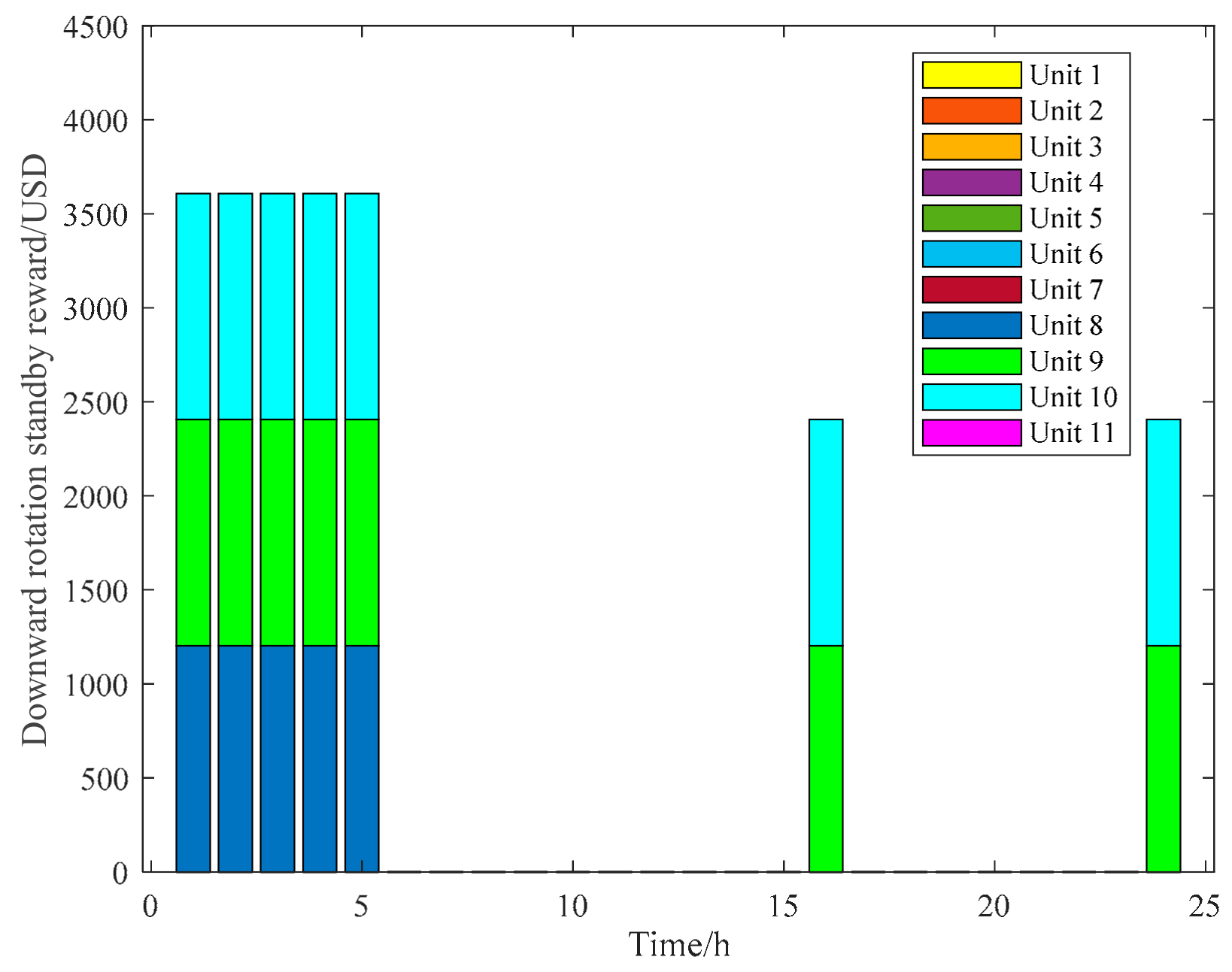
3.3. Analysis of Backup for Deterministic Wind Power

The system operating costs for the four scenarios based on the wind power forecast values (Circumstance 3) are shown in

Table 6. Statistics of operating results based on wind power prediction values.

Cost/USD	Scenario 1	Scenario 2	Scenario 3	Scenario 4
Fuel	156,945	157,073	151,045	151,286
Abandoned wind	3290	3290	7328	7328
Reducible load	3768	3768	4264	4264
Start-up and shutdown	2076	2076	1984	1984
Synchronized reserve	21,932	12,908	20,580	12,635
Operating before assessment	188,011	179,115	185,201	177,497
Upward synchronization backup penalty	13,355	6878	11,971	6785
Downward synchronization backup penalty	5086	4968	7129	5849
Downward synchronization standby reward	8168	7394	26,236	22,853
Backup after assessment	32,204	17,360	13,443	2416
Operation after assessment	198,282	183,567	178,064	167,278

. In the first stage of start–stop optimization without considering operational risk, the optimization of standby cost for Scenario 2 compared to Scenario 1 results in a reduction in system standby cost by USD 9024. In the first stage of start–stop optimization with operational risk, Scenario 4 vs. Scenario 3, the optimization of standby cost reduces the system standby cost by USD 7945, and in the second stage of optimization with simultaneous standby optimization, Scenario 4 vs. Scenario 2 reduces the total pre-evaluation operating cost by USD 1618. Therefore, with the wind power forecast lower limit as the benchmark, Scenario 4 achieves the efficient allocation of system standby resources and optimal economic scheduling of the system by considering the two-phase optimization of start–stop, conditional risk, and synchronous standby.

Table 6 analyzes the costs after the application of the proposed auxiliary standby market assessment model for settlement. The first-stage optimization model optimally allocates the start/stop states and optimal output of each unit, resulting in the optimal total cost of backup after evaluation. Scenarios 3 and 4 are significantly better than Scenarios 1 and 2, where the corresponding lower synchronized standby reward costs exceed USD 20,000 each. The second stage of synchronized standby optimization effectively coordinates the system unit output and synchronized standby capacity to obtain an optimal configuration strategy, and the results show that Scenario 4 is significantly better than Scenario 3, and Scenario 4 has a lower up-synchronized standby penalty cost and a lower down-synchronized standby penalty cost, which reduces the evaluated total standby cost by USD 11,027 and also reduces the evaluated total operating cost by USD 10,786.

Looking at the overall evaluation results, the reward benefits of Scenario 3 are not sufficient to cover its total up and down synchronization standby penalty costs. Scenario 4 has total post-evaluation standby cost savings of USD 11,027 compared to Scenario 3. The total post-evaluation operating cost savings were USD 10,786.

3.4. Operation Cost Analysis of Three Circumstances Based on Scenario 4

Table 7. Comparison of uncertainty and renewable integration cost.

Cost/USD	Predictive Values	Upper Limit of Wind Power Prediction Values	Lower Limit of Wind Power Prediction Values
Fuel	151,286	150,736	151,875
Abandoned wind	7328	7306	7552
Reducible load	4264	4266	4264
Start-up and shutdown	1984	1984	1984
Synchronized reserve	12,635	12,665	12,596
Operating before assessment	177,497	176,957	178,271
Upward synchronization backup penalty	6785	6803	6765
Downward synchronization backup penalty	5849	5863	5831
Downward synchronization standby reward	22,853	22,846	22,849
Backup after assessment	2416	2485	2344
Operation after assessment	167,278	166,777	168,019

presents the uncertain renewable energy operating cost results for Scenario 4 for the three circumstances. From the results, it is found that the lowest total operating cost of USD 166,777 is the ideal best scenario when the upper limit of wind power forecast is the input value, which is evaluated by the two-stage optimized standby ancillary services market.

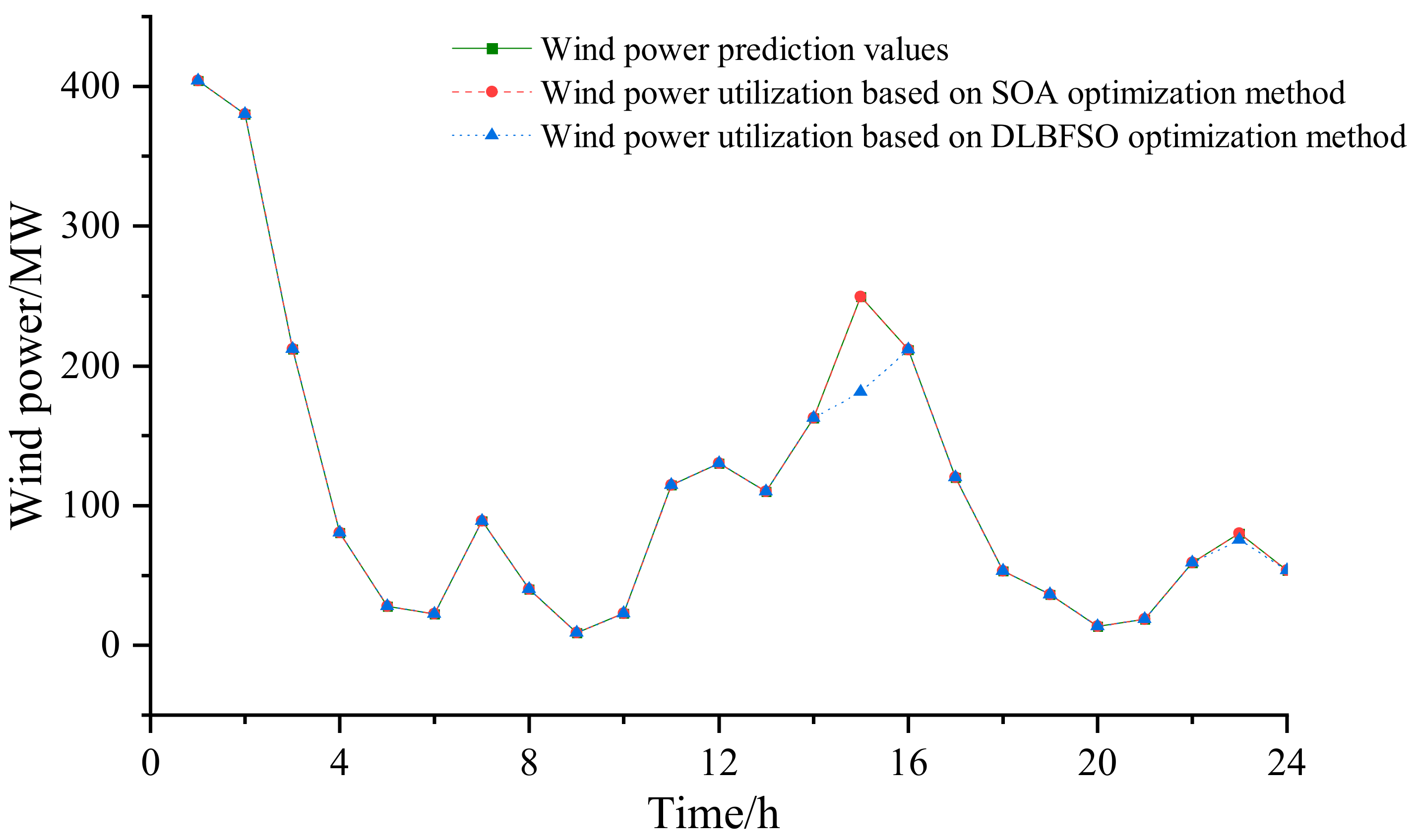
3.5. Analysis of the Running Results of Two Optimization Algorithms Based on the Optimal Scenario

Table 8. Comparison of scenario 4 based on predicted values.

Cost/USD	Scenario 4 (DLBFSO)	Scenario 4 (SOA)
Fuel	150,736	146,935
Abandoned wind	7306	0
Reducible load	4266	5400
Start-up and shutdown	1948	1924
Synchronized reserve	12,665	12,702
Operating before assessment	176,957	166,961
Upward synchronization backup penalty	6803	6840
Downward synchronization backup penalty	5863	5862
Downward synchronization standby reward	22,846	31,949
Backup after assessment	2485	−6545
Operation after assessment	166,777	147,714

shows the results of Scenario 4 based on the wind power prediction upper limit (Circumstance 1). By comparing the optimization results of the DLBFSO algorithm and the SOA algorithm, the total operating cost of the SOA algorithm is reduced by USD 19,063 compared to the DLBFSO algorithm, indicating that the SOA optimization algorithm has better performance. The main influencing factors are the cost of wind abandonment and the cost of synchronized backup rewards. Figure 16 and Figure 17 show a comparison of the cost allocation results for synchronous backup rewards under two optimization algorithms. Figure 18 shows a comparison of wind power utilization rates between two optimization algorithms.

4. Conclusions

In this paper, a two-stage optimal scheduling strategy taking into account operational risk and standby economics is proposed, and a standby auxiliary service market reward and punishment assessment model is established. By improving the new power system of the IEEE30 node as an arithmetic example and designing a comparative analysis of three circumstances corresponding to four scenarios, the feasibility and effectiveness of the proposed method are verified, and the following conclusions are drawn:

1.

The data-driven wind power prediction based on the upper bound circumstance (Circumstance 1) corresponding to the simultaneous consideration of start–stop optimization and standby optimization (Scenario 4) has the lowest total cost of operation and the best optimization results.

2.

Based on the lowest optimization cost results (Circumstance 1, Scenario 4), DLBFSO is used to compare with SOA optimization algorithms, and it is found that SOA optimization methods have the lowest running cost and the best optimization results.

Through the effective mechanism of the standby auxiliary service market, this provides flexibility, stability and economic support to the new power system, which can effectively cope with load fluctuations and sudden failures, reduce the risk of the new power system, promote the efficient use of clean energy, facilitate market competition, realize the sustainable development of the new power system, and provide users with reliable and economic power services.

References

1. Yun, Y.; Dong, H.; Chen, Z.; Huang, R.; Ding, K. A two-stage stochastic scheduling optimization for multi-source power system considering randomness and concentrating solar power plant participation. Power Syst. Prot. Control. 2020, 48, 30–38. [Google Scholar]
2. Deng, T.; Lou, S.; Tian, X.; Wu, Y.; Li, N. Optimal dispatch of power system integrated with wind power considering demand response and deep peak regulation of thermal power units. Autom. Electr. Power Syst. 2019, 43, 34–41. [Google Scholar]
3. Li, P.; Yu, D.; Yang, M.; Wang, J. Flexible look-ahead dispatch realized by robust optimization considering CVaR of wind power. IEEE Trans. Power Syst. 2018, 33, 5330–5340. [Google Scholar] [CrossRef]
4. Jin, H.; Sun, H.; Niu, T.; Guo, Q.; Wang, B. Coordinated dispatch method of energy-extensive load and wind power considering risk constraints. Autom. Electr. Power Syst. 2019, 43, 9–16. [Google Scholar]
5. Zhou, X.; Li, W.; Tang, J.; Wang, Q.; Yu, J.; Zhang, C. Coordinated allocation method of emergency reserve capacity based on risk Quantification. Power Syst. Technol. 2015, 39, 1927–1932. [Google Scholar]
6. Ai, X.; Taierjiang, B.; Yang, L.; Yang, J.; Fang, J.K.; Wen, J. Spinning reserve optimization of wind power system based on Scenario set. Power Syst. Technol. 2018, 42, 835–841. [Google Scholar]
7. Wang, J.; Xu, J.; Wang, J.; Ke, D.; Liao, S.; Sun, Y.; Wu, Y.; Bi-level Stochastic Optimization for A Virtual Power Plant Participating in Energy and Reserve Market Based on Conditional Value At Risk. Power System Technology, 2024, Web First Paper. Available online: https://kns.cnki.net/kcms2/article/abstract?v=wcPNn8Zia7NoLxS3GYI68UUmlF1-VOKNbfcttOWGuaZHtAYMFQhmPE9L_SuNFLk243PVObkGWwo6XtyCq0SmEDOjO0rxfRm57TSG0-xHzziIr-KQe_OPnm0pFTMkHEoIh8kihZIqlhs=&uniplatform=NZKPT&language=CHS (accessed on 11 January 2021).
8. Yan, B.; Han, X.; Li, T.; Song, T.; Wu, Y. Operation Strategy for Active Distribution Networks with Energy Storage Considering. Autom. Electr. Power Syst. 2023, 47, 131–140. [Google Scholar]
9. Yan, M. Electricity values equivalent pricing system and relevant systems design: Part four a probabilistic practical electricity values equivalent pricing method for operating reserve. Autom. Electr. Power Syst. 2023, 27, 1–6. [Google Scholar]
10. ERCOT. Methodology for Implementing ORDC to Calculate Real Time Reserve Price Adder [EB/OL]. Available online: https://www.ercot.com/content/wcm/training_courses/107/ordc_workshop.pdf (accessed on 11 January 2021).
11. Summary of 2019 MISO State of the Market Report; Potomac Economics: Fairfax, VA, USA, 2020.
12. Hogan, W. Strengths and Weaknesses of the PJM Market Model [EB/OL]. Available online: https://scholar.harvard.edu/whogan/files/hogan_chapter_7_handbook_on_the_economics_of_electricity_112619r.pdf (accessed on 2 November 2019).
13. Hogan, W. On an ‘Energy only’ Electricity Market Design for Resource Adequacy; Harvard University: Cambridge, MA, USA, 2005. [Google Scholar]
14. ERCOT. ERCOT Market Training: Purpose of ORDC, Methodology for Implementing ORDC, Settlement Impacts for ORDC [EB/OL]. Available online: http://www.ercot.com/content/wcm/training_courses/107/ordc_workshop.pdf (accessed on 11 January 2021).
15. Maggio, D.; Moorty, S.; Shaw, P. Scarcity Pricing Using ORDC for Reserves and Pricing Run for out of Market Actions [EB/OL]. Available online: https://cdn.misoenergy.org/20210513%20MSC%20Item%20XX%20Scarcity%20Pricing%20Evaluation%20Paper550162.pdf (accessed on 11 January 2021).
16. Liu, R.; Jing, Z.; Liu, Y. Coupling clearing model of energy and reserve considering dynamic operation reserve demand curves. Autom. Electr. Power Syst. 2021, 45, 34–42. [Google Scholar]
17. Harbord, D.; Pagnozzi, M. Britain’s electricity capacity auctions: Lessons from Colombia and New England. Electr. J. 2014, 27, 54–62. [Google Scholar] [CrossRef]
18. Jing, R.; Zhou, Y.; Wu, J. Empowering zero carbon Future-experience and development trends of electric power system transition in the UK. Autom. Electr. Power Syst. 2021, 45, 87–98. [Google Scholar]
19. ENTSO-E. Frequency Containment Reserve [EB/OL]. Available online: https://www.entsoe.eu/network_codes/eb/fcr/ (accessed on 11 January 2021).
20. PJM. PJM Manual 11: Energy & Ancillary Services Market Operations [EB/OL]. Available online: https://citeseerx.ist.psu.edu/document?repid=rep1&type=pdf&doi=200ce69f3ee2eea1f26897043555710ea30342cd (accessed on 11 January 2021).
21. Zhu, J.; Ye, Q.; Zou, J.; Xie, P.; Xuan, P. Short-term operation service mechanism of ancillary service in the UK electricity market and its enlightenment. Autom. Electr. Power Syst. 2018, 42, 1–8. [Google Scholar]
22. Zhang, G.; Li, F. Two-stage optimal dispatch for wind power integrated power system considering operational risk and reserve availability. Power Syst. Prot. Control. 2022, 50, 140–148. [Google Scholar]
23. Kou, Y.; Wu, J.; Zhang, H.; Yang, J.; Jiang, H. Low carbon economic dispatch for a power system considering carbon capture and CVaR. Power Syst. Prot. Control. 2023, 51, 132–140. [Google Scholar]
24. Liu, H.; Gao, X.; Liu, Y. Two-stage Day-ahead Optimal Dispatching of Active Distribution Network Based on Improved Artificial Fish Swarm Algorithm. Guangdong Electr. Power 2023, 36, 123–129. [Google Scholar]
25. Zhang, S.; Zhang, J. Wind Power Load Combination Forecasting Based on Improved SOA and Ridge Regression Weighting. North China Electr. Power Univ. 2023, Web First Paper. Available online: https://kns.cnki.net/kcms2/article/abstract?v=wcPNn8Zia7P6dqHCTULDrCKVHV66YLQTTGJr8zUnFYKT4pFkiTxnBTct6g-cJPuY7SXwli8QMKHqv1-wezPH5JV9J3dnUPBlLSHWRZ7ySJZgGbZwi8JDGecQNXKkwvpeHUE3IYXXl68=&uniplatform=NZKPT&language=CHS (accessed on 11 January 2021).
26. Sun, H.; Song, Y.; Chen, L.; Peng, C.; Jiang, Z. Source-grid coordination security and economic dispatching of new power system considering reserve risk. Electr. Power Autom. Equip. 2024, 44, 135–143. [Google Scholar] [CrossRef]
27. Shui, Y.; Liu, J.; Gao, H.; Huang, S.; Jiang, Z. A Distributionally Robust Coordinated Dispatch Model for Integrated Electricity and Heating Systems Considering Uncertainty of Wind Power. Proc. CSEE 2018, 38, 7235–7247. [Google Scholar]
Figure 1. Workflow diagram.
Energies 17 01921 g001
Figure 2. Wind power prediction results.
Energies 17 01921 g002
Figure 3. Monte Carlo simulation load curve.
Energies 17 01921 g003
Figure 4. System total load forecasting curve.
Energies 17 01921 g004
Figure 5. Optimization results of synchronous standby scenarios in view of the upper limit of wind power values.
Energies 17 01921 g005
Figure 6. Upward synchronous reserve capacity of Scenario 4 based on the upper limit of wind power values.
Energies 17 01921 g006
Figure 7. Upward synchronous reserve capacity of Scenario 3 based on the upper limit of wind power values.
Energies 17 01921 g007
Figure 8. Downward synchronous reserve capacity of Scenario 4 based on the upper limit of wind power values.
Energies 17 01921 g008
Figure 9. Downward synchronous reserve capacity of Scenario 3 based on the upper limit of wind power values.
Energies 17 01921 g009
Figure 10. Upward synchronization standby penalty cost of Scenario 4 based on the upper limit of wind power values.
Energies 17 01921 g010
Figure 11. Upward synchronization standby penalty cost of Scenario 3 based on the upper limit of wind power values.
Energies 17 01921 g011
Figure 12. Downward synchronization standby penalty cost of Scenario 4 based on the upper limit of wind power values.
Energies 17 01921 g012
Figure 13. Downward synchronization standby penalty cost of Scenario 3 based on the upper limit of wind power values.
Energies 17 01921 g013
Figure 14. Downward synchronous reserve reward of Scenario 4 based on the upper limit of wind power values.
Energies 17 01921 g014
Figure 15. Downward synchronous reserve reward of Scenario 3 based on the upper limit of wind power values.
Energies 17 01921 g015
Figure 16. Downward synchronous reserve reward of Scenario 4 based on the upper limit of wind power values (DLBFSO).
Energies 17 01921 g016
Figure 17. Downward synchronous reserve reward of Scenario 4 based on the upper limit of wind power values (SOA).
Energies 17 01921 g017
Figure 18. Comparison of Wind Power Utilization based on DLBFSO and SOA Optimization Methods.
Energies 17 01921 g018