Article

Breaking Borders with Joint Energy and Transmission Right Auctions—Assessing the Required Changes for Empowering Long-Term Markets in Europe †

Electa Department, University of Leuven/Energyville, 3001 Heverlee, Belgium
*
Author to whom correspondence should be addressed.
This paper is an extended version of our paper published in 7th AIEE Energy Symposium: Current and Future Challenges to Energy Security—The Energy Crisis, the Impact on Transition Roadmap, Virtual Conference, 14–16 December 2022; pp. 136–168.
Energies 2024, 17(8), 1923; https://doi.org/10.3390/en17081923
Submission received: 2 February 2024 / Revised: 1 April 2024 / Accepted: 9 April 2024 / Published: 17 April 2024
(This article belongs to the Section C: Energy Economics and Policy)

Abstract

:
The establishment of a long-term, cross-border market in which forward market coupling and bilateral contracts are developed in an integrated approach is instrumental for the European internal electricity market. We propose the joint energy and transmission right auction (JETRA) mechanism, developed by O’Neill et al., as a solution for long-term cross-border markets in Europe. The main contribution of this research lies in its examination of the underlying market structures for effective JETRA implementation. We compare the institutional setting, market rules, and grid modeling under nodal and zonal pricing systems, adapting JETRA to the flow-based market coupling (FBMC) mechanism that is currently implemented in the European day-ahead market. This adaptation reveals the inherent limitations of FBMC in supporting JETRA, in particular in the long-term auction. We also identify constraints posed by existing European market rules, particularly those that affect the application of multi-settlement rules and the effective timeframe of hedging instruments. In conclusion, our research suggests that transitioning from zonal to nodal pricing is essential for JETRA’s effective implementation. Furthermore, a comprehensive market reform is required to seamlessly integrate long- and short-term markets.

1. Introduction

1.1. Policy Context

The societal drive for decarbonization and the need to hedge against spot market volatility call for the development of a long-term, cross-border market in Europe. The most recent European energy legislation is called the REPowerEU package, which includes initiatives such as energy savings, energy supply diversification, and the accelerated rollout of renewable energy [1]. In particular, the renewable target for 2030 is expected to increase from 40% to 45%. Tapping the potential of renewable energy resource complementarity over large geographical areas with a cross-border electricity market is essential for the establishment of an optimized, reliable, and low-cost energy system in Europe. It is crucial to note that the focus of electricity wholesale market development has shifted from short-term competition to long-term market instruments. In the wake of the recent energy crisis, the significance of stable prices from forward markets for consumers as well as hedging instruments to shield them from spot market volatility is still greater. In the zero-subsidy era, renewable power purchase agreements (PPAs) are also popular in the long-term market. Essentially, renewable PPAs are bilateral contracts between renewable suppliers and demands; thus, they can generate stable cash flows for renewable investors and meet consumers’ demand for low-cost green electricity.

1.2. Current Status of the Long-Term, Cross-Border Market in Europe

In recent years, renewable PPAs have been on the rise within national borders. In Europe, the contracted PPA volume grew from 3.86 GW in 2018 to 8.46 GW in 2022 [2]. However, to the best of our knowledge, there are no public examples of cross-border physical PPAs in Europe. The 2023 electricity market reform proposal from the European Commission also recognizes the importance of long-term contracts [3].
Establishing cross-border transmission rights that hedge against congestion cost risk is crucial for the success of cross-border bilateral contracts. Commission Regulation 2016/1719 requires transmission system operators (TSOs) to develop harmonized rules for allocating long-term physical and financial transmission rights (FTRs) [4]. Currently, TSOs allocate long-term, cross-border transmission rights to market players through an explicit auction, where the interconnection capacity is separately procured from energy contracts. The duration of long-term transmission rights is up to one year, which does not match the length of PPAs. A conflict of interest arises when traders seek to acquire more transmission capacity in the long-term while TSOs seek to distribute it more equally across different timeframes [5].
An organized forward market is an important part of the electricity market that complements the competitive spot market. Currently, day-ahead and intra-day markets are coupled in Europe. The recent energy crisis demonstrates that consumers who are not hedged can be exposed to sometimes high and highly volatile spot market prices.
Coupling the forward market to provide long-term energy contracts from the wholesale market, which implicitly includes transmission access, is the next natural step in the market coupling process. In its recent consultation announcement, the Agency for the Cooperation of Energy Regulators (ACER) recognized the flow-based approach as an efficient methodology for the allocation of long-term transmission rights, in which the physical reality of the network elements is considered while calculating energy exchange between borders [6].
In the electricity market reform proposal from the European Commission, PPAs and forward markets are recognized as measures of long-term market development [3]. The historical case of the regional transmission organization (RTO) PJM in the U.S. suggests that when subject to zonal pricing, grid constraint costs were not adequately presented to market players. The price difference between wholesale energy and bilateral contracts led to a surge in bilateral contracts, resulting in severe grid congestion in the summer of 1997, which consequently prompted the administrative prohibition of such contracts to ensure grid reliability [7]. In this research, we advocate the establishment of a long-term cross-border market that is compatible with both bilateral and wholesale energy contracts. The long-term market discussed in this paper refers to organized markets or bilateral transactions more than one year ahead of electricity delivery, for example, 3 to 5 years prior to real-time operation.

1.3. Literature Review and Research Gap

In the existing literature, topics such as forward market coupling, long-term transmission rights, the FBMC mechanism, and the transition from zonal pricing to nodal pricing in the European electricity market are often discussed separately in distinct contexts. Jamasb et al. highlighted the role of long-term contracts and markets in hedging against short-term price volatility [8]. They explored various policy options for long-term markets, including renewable PPAs, contracts of differences (CfDs), and mandatory quotas for long-term market participation.
D’Aertrycke and Smeers investigated whether transmission rights allocated under Transfer Capacity (TC) and FBMC mechanisms uphold the properties of superposition and netting [9]. Notably, the analysis of the non-linearity of generation shift keys (GSKs) reveals limitations of the FBMC methodology, which only supports superposition and nettting properties for linear GSKs. Furthermore, D’Aertrycke and Smeers proposed two criteria to evaluate the feasibility of transposing FTRs from a nodal pricing system to a zonal one. Their analysis concludes that this transposition presents a significant challenge.
  • The first criterion concerns the satisfaction of superposition and netting properties. Since these properties cannot always be guaranteed in the short-term market due to the non-linearity of GSKs, the authors infer that they would also fail in the long-term market.
  • The second criterion focuses on the firmness of FTRs under FBMC. A critical challenge for achieving FTR firmness lies in the simultaneous feasibility test under FBMC, which would require the set of transmission rights allocated in the forward market to be feasible for the day-ahead zonal PTDF. This necessitates information about both grid topologies and generation demand shift keys (GDSK) in the day-ahead market. However, GDSKs are not available in the forward market, and acquiring this information is not the responsibility of TSOs, even if it exists.
There are two key distinctions between the concept of firmness explored in our paper and the discussion in D’Aertrycke and Smeers’ paper. Firstly, the authors referenced the allocation of FTRs in the current U.S. market, which only involves a portfolio of FTRs. In contrast, our paper addresses the joint allocation of FTRs, Physical transmission rights (PTRs), and energy rights in the forward market. Secondly, the JETRA mechanism imposes two requirements for ensuring the physical feasibility of auctioned rights in subsequent rounds. First, transmission constraints must be satisfied in each round. Second, the PTDFs in subsequent auction rounds must be less than or equal to those in earlier rounds, and the flow limits in the previous round must be less than or equal to those in the subsequent rounds. A more detailed discussion can be found in Section 4.2.
Spodniak et al. constructed a combination of electricity price area differentials (EPAD comb) to simulate FTR pricing in the Nordic electricity market and compared these future prices with spot market prices [10]. They observed a negative ex-post risk premium for most interconnections, raising questions regarding FTR demand and the validity of these hedging products in the Nordic market. From a cost and risk allocation perspective, Beato emphasized the differing incentives of TSOs and transmission users concerning the development of long-term transmission-right products [11]. Unless the TSOs are guaranteed cost recovery from their regulators, they would be reluctant to increase the quantity and duration of long-term transmission rights. Additionally, TSOs are required to ensure the firmness of long-term transmission rights, or they must compensate the right holders and face the risk of these costs not being approved for reimbursement through network tariffs.
Meanwhile, the literature on FBMC mainly focuses on explaining its grid modeling parameters and assessing its performance in short-term markets [12,13]. Regarding zonal pricing, Purchala criticized the current market design based on zonal pricing and advocated for a shift towards nodal pricing [14]. This paper outlines several drawbacks of the current zonal pricing system in Europe, including: (1) low utilization of cross-border network capacity; (2) decoupled market and system operation; (3) increased need for redispatch measures; (4) opportunities for market players to strategically game the system operator; and (5) insufficient price signals to facilitate generation adequacy. Eicke and Schittekatte discussed the six primary arguments used by European stakeholders to counter the nodal pricing implementation in Europe. They provided counterarguments or mitigation options to address these concerns, which include market power, barriers to unlocking flexibility, market liquidity issues, investment risk, complexity, and locational price differentiation [15].
This research aims to bridge the knowledge gap in the literature by (1) introducing the joint energy and transmission right auction (JETRA) as the mechanism for the long-term, cross-border electricity market and (2) examining whether the current FBMC design and institutions are compatible for implementing JETRA effectively [16]. It is expanded from the previous work by Huang and Deconinck [17].

1.4. Research Questions and Scope

In light of the need and challenges associated with the development of long-term markets in Europe, the following research questions are explored:
  • What could be an effective mechanism for developing long-term transmission rights and forward market coupling?
  • Is the zonal pricing-based FBMC currently implemented in the European cross-border market conducive to establishing the proposed long-term market?
  • Are current institutional settings fit for purpose?
Assuming an equal emphasis on the two forms of contracts in the long-term timeframe, this research proposes that cross-border bilateral contracts and forward market coupling should be promoted in an integrated manner. This approach suggests that similar to the existing day-ahead market coupling, wholesale energy contracts that implicitly incorporate cross-border transmission access for market players should be included in the long-term market. Furthermore, bilateral contractual arrangements in the long-term market, such as PPAs, should be supported through the auction of financial and physical transmission rights to help market participants fulfill contractual delivery obligations.
A central issue in the co-development of the two contract forms is the allocation of cross-border transmission capacity. Therefore, we propose the JETRA model developed by O’Neill et al., which optimizes systematic transmission usage for wholesale energy contracts and transmission rights that support bilateral contracts, as the primary mechanism for the long-term market. JETRA operates in multiple market timeframes and auctions various hedging products, such as financial and physical transmission rights as well as energy purchase and sale, which implicitly include transmission access [16]. Furthermore, it connects market outcomes across different timeframes using multi-settlement rules to help market players hedge against spot market volatilities.
While an effective market mechanism is crucial for facilitating long-term, cross-border electricity trading, it alone does not guarantee the efficient application of JETRA. The underlying market structure where JETRA is implemented plays a critical role in its effectiveness. Understanding the interlinkage between institutional functions, grid modeling, and market rules across different timeframes and their implications for JETRA’s effectiveness could inform holistic policy design and guide future market reform directions.
Several key considerations arise when evaluating the compatibility of JETRA within the current zonal pricing market in Europe. JETRA, under nodal pricing, is implemented as a centralized auction in which the SO has access to market bid information and network data needed for system optimization. However, FBMC, under zonal pricing, adopts a decentralized market structure in which TSOs and power exchanges interact to clear the market. The inefficiencies stemming from information asymmetry between the TSO and market players are discussed in the literature for the flow-based market coupling implementation in the short-term market [14,18]. TSOs compute grid models prior to market opening without bid information. Therefore, the input parameters for FBMC grid modeling, which should be a result of market clearing, are predictive in nature and require the TSOs to forecast energy injection and withdrawal patterns.
In the long-term auction, JETRA, with its multiple products and multi-settlement rules, gives market players the flexibility of options to combine different hedging products with spot market trade. Furthermore, there is a long lead time prior to energy delivery, which implies potential for generation investments and load shifting. Compared with energy bids in the day-ahead market that reflect generation and load patterns, there are more combinations and possibilities of bids in the JETRA auction. Therefore, JETRA implementation under FBMC in the long-term creates higher information needs for zonal grid modeling, which is linked to the auction clearing outcome. The intensified information needs and predictive nature of the FBMC grid parameters imply higher uncertainties for JETRA grid modeling under FBMC compared with the currently implemented day-ahead FBMC.
On the hedging mechanism and settlement rules, the JETRA design reflects and builds upon some U.S. market experience, including PJM and the New York market [16]. These markets feature integrated energy and transmission auctions in both day-ahead and real-time markets, where locational marginal pricing is applied. The day-ahead market serves as a forward market. While only the real-time market, which clears 5–10 min before electricity delivery, represents physical dispatch. Energy bids in the day-ahead market are financial and settled in the real-time market. The final iteration of the original JETRA design, in which the energy and transmission rights are ultimately settled, represents physical dispatch and corresponds to the real-time market.
In the European context, the day-ahead market is regarded as a spot market that involves physical dispatch. Both the day-ahead and intra-day markets adopt zonal pricing, employing an aggregated zonal network model to clear the market. After the gate closure of spot markets, TSOs assess grid feasibility and perform redispatch to alleviate grid congestion. From the day-ahead market onwards, the allocation of transmission capacity is sequential. These differences in market structure are crucial when considering how the long-term market can be related to the short-term market, as well as how the energy and transmission rights market players have procured from the long-term market can eventually be settled.
This paper identifies two potential challenges associated with implementing JETRA under FBMC. Firstly, we posit that increased uncertainties in JETRA grid modeling, in particular within the long-term auction, could amplify inefficiencies in the FBMC methodology in JETRA implementation under FBMC. Secondly, the interplay between physical dispatch from the day-ahead market and sequential allocation of transmission capacity in the European market might limit the applicability of multi-settlement rules, potentially impacting hedging effectiveness and cross-border cooperation. To verify these hypotheses, a stylized network is established to showcase the JETRA implementation under zonal pricing and compare its performance with nodal pricing.
On grid modeling, by analyzing in depth the computation process of FBMC, we highlight how the high uncertainties bring significant challenges to the computation of FBMC grid parameters and generate inefficient dispatch outcomes. Specifically, by assessing the role of information asymmetry between TSOs and market bidders in the grid modeling stage, we demonstrate how the methodological dilemma of JETRA implementation is linked to institutional functions inherent in zonal pricing. Through delving into the application of multi-settlement rules and their relationship with physical and financial dispatch, the analysis uncovers how the combination of physical dispatch and sequential allocation of transmission capacity from the day-ahead market restricts the application of multi-settlement rules and limits hedging effectiveness in the European context.

1.5. Paper Organization

The remainder of the paper is organized as follows: Section 2 describes the JETRA optimization formulation as well as the case study setting. Section 3 describes the institutional settings for JETRA under nodal and zonal pricing, the spatial and temporal dimensions of the market design, and the application of the multi-settlement rule. Section 4 provides an in-depth discussion of the grid modeling challenges of JETRA implementation following the FBMC methodology. Section 5 first presents JETRA implementation under nodal pricing. Next, it describes how the key grid parameters under FBMC are set for JETRA implementation in the case study. Subsequently, it presents the JETEA calculation steps and settlement outcomes under FBMC mechanisms in different timeframes. In Section 6, a set of indices is proposed for evaluating the joint auction outcomes. Afterwards, the case study’s performance under nodal and zonal pricing is compared. Lastly, Section 7 concludes the research findings and deduces policy implications.

2. Joint Energy and Transmission Right Auction Model

In this section, we present the JETRA model and explain why its features are desirable for long-term, cross-border market development in Europe. Section 2.1 describes the JETRA formulation, its wide range of hedging instruments, and the function of multi-settlement rules that link market outcomes in different timeframes. In Section 2.2, a case study is presented with a stylized network typology and several types of bids.

2.1. JETRA: A Recipe for Long-Term Market Development

This research proposes the joint energy and transmission right auction as the primary mechanism for co-developing cross-border bilateral contracts and forward market coupling.
The mathematical formulation of the auction model can be found in Appendix A. The objective of the joint energy and transmission rights auction model is to maximize the value of accepted bids, which includes point-to-point financial transmission rights, flow gate rights, and energy sale/purchase contracts. Constraints for this auction optimization include the load flow constraint and the energy balance between supply and demand. Bidders must submit their offer prices and specify the lower and upper constraints for the quantities they bid for energy sale/purchase and transmission rights.
To maintain revenue adequacy for the system operator (SO), the nodal power transfer distribution factor (PTDF) values used in the grid model of the initial auction rounds must be larger than or equal to those of the later auctions. At the same time, the flow limits of the transmission network in the preceding auctions should be smaller than or equal to those of the later auctions. In this study, only DC load flow constraints are used. The network topology remains consistent across different timeframes.
The model is proposed for the European cross-border electricity market because it has several desirable features, which are detailed in the following subsections:

2.1.1. A Wide Range of Hedging Instruments

This auction design provides network users with the flexibility to choose hedging instruments that encompass energy and transmission rights and facilitates the adjustment of their positions across different timeframes. The wholesale energy market, including energy supply and demand bids with implicit transmission access, can be brought to the forward market timeframe before the day-ahead market.
If prices fluctuate between locations, bilateral contract holders must hedge against congestion charges, which are the product of energy volume and price differences between injection and withdrawal locations. The inclusion of transmission rights as congestion hedging tools in joint auctions enables large-scale, long-term bilateral contracts across borders. Oren provided an overview of financial transmission rights (FTRs) and physical transmission rights (PTRs), both of which are included in JETRA [19]. They are defined as follows:
  • FTRs are forward contracts that entitle their holders to the right to receive locational marginal price differences between the specified withdrawal and injection points during a specified time interval [20]. From a market player’s perspective, holding FTRs allows them to pay congestion charges based on nodal differences, regardless of the power flow distribution through the network. When coupled with long-term contracts, FTR can provide market players with a perfect hedge against spot price volatility. The allocation of FTRs requires a central view of network conditions from the SO.
  • PTRs give their holders the right to collect the shadow price of the specified transmission element in accordance with the specified direction and time interval [21]. To hedge against locational price differences, a PTR portfolio must be composed and weighted for each transmission path associated with the underlying energy contract. Thus, it requires an accurate calculation by the user of the transmission path usage for the intended transaction. Market players can bid PTR for the most likely congested transmission network element to hedge a portion of the congestion risk or to collect congestion rent. PTRs alone can be allocated without a central auction, as the physical limits of certain transmission elements can be individually determined by the owners of network assets.

2.1.2. The Multi-Settlement Rules

The multi-settlement rule stipulates that bid winners earn their revenues or make payments based on the volumes determined in the previous auction and the prices set by the bids in the current auction. For instance, if a market player has a bilateral contract of 100 MWh and procures 100 MWh of FTRs between the specific node pair that corresponds to the bilateral contract at €5/MWh in the three-year-ahead auction, then €500 is paid to the SO to obtain these rights. In the subsequent auction, which could be a year or month ahead, if the FTR price rises to €10/MWh, then the market player will receive €1000 from the SO for the 100 MWh FTR.
This implies that market participants who have secured energy contracts or transmission rights in a previous auction round will receive the amount necessary to procure the same quantity of energy or transmission rights in the current auction. Consequently, the market player can always maintain their initial hedging quantity by acquiring new rights in a subsequent auction without incurring additional costs to hedge against spot market price volatility. In the final auction round, physical dispatch can be made, which means that market clearing is associated with the actual energy delivery [22].
A salient characteristic of the multi-settlement rule is that in each subsequent auction round, the outcome of the previous auction, (i.e., the allocated energy and transmission rights) is liquidated. This implies that all financial positions maintained by right holders are subsequently bought back or sold back. During real-time dispatch or the last auction round, the SO can optimize network usage in line with the operating conditions.
Liquidation implies that the auction outcome is financially binding but does not hold physical commitment in the market timeframes leading up to the final settlement. Before the era of electricity liberalization, long-term priority interconnection access was prevalent, which could be used to monopolize essential facilities and potentially discriminate against competitors [23]. Such anticompetitive concerns that arise from the physically binding interconnection priority right do not apply to JETRA.
In conclusion, the extensive selection of instruments that span both energy and transmission products, the flexibility afforded to market players in determining their preferred hedging mechanisms, and the consistent market settlement rules across timeframes make JETRA a compelling proposition for developing a long-term, cross-border European electricity market.

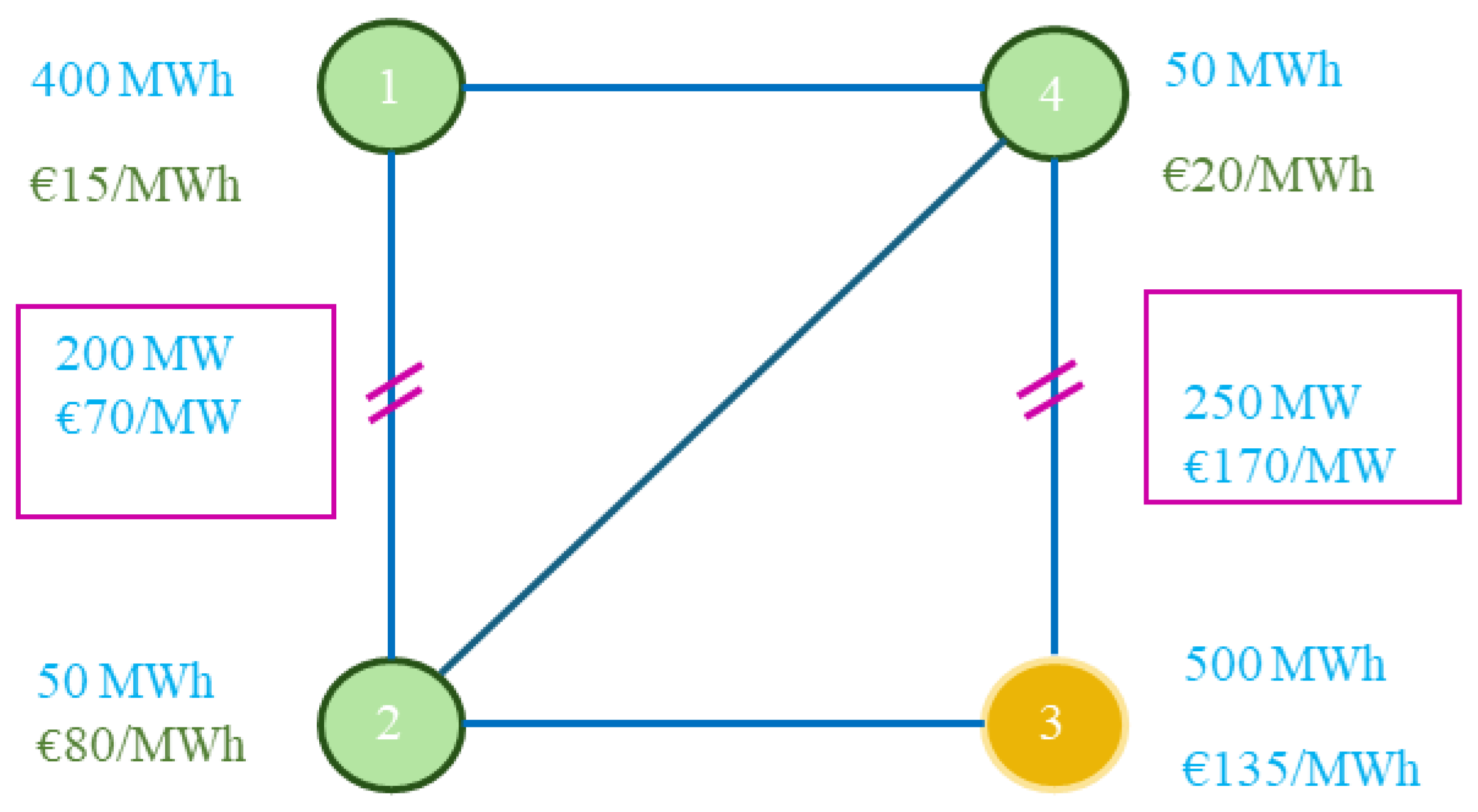
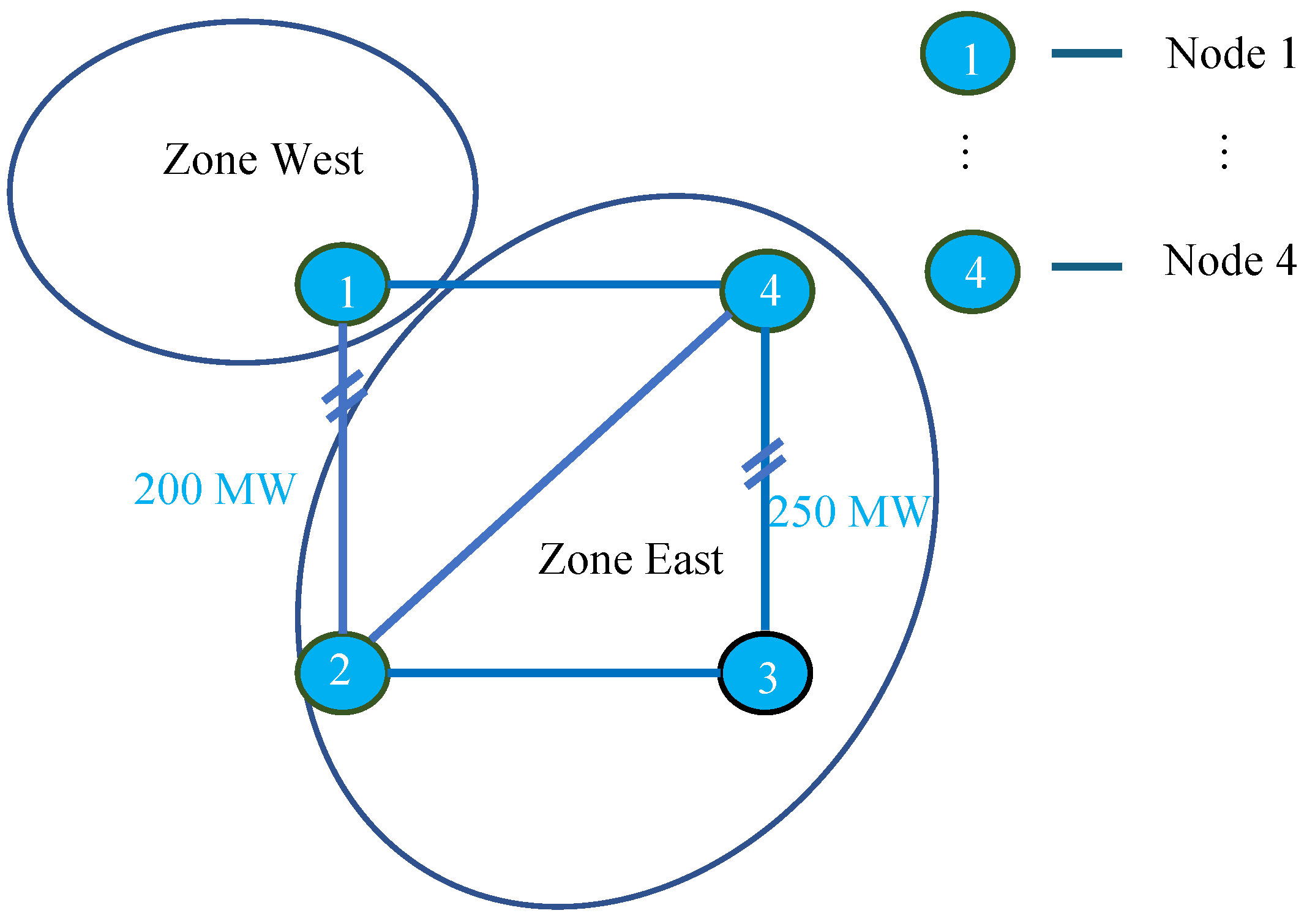
2.2. Case Study Network and Bids

A case study is formulated using the network illustrated in Figure 1. Each line shares the same impedance. The network capacity limit of lines 1–2 is 200 MW, while that of lines 4–3 is 250 MW. All other lines have a capacity limit of 400 MW. The network has four nodes. Given this network topology and the maximal demand, which in this case study is 500 MWh, the maximal physical flow on any transmission element will not exceed 312.5 MW (calculated as 500 × 0.625, 0.625 being the highest nodal PTDF value of node pairs between zone west and zone east). Lines with a capacity of 400 MW can be perceived as transmission elements without capacity constraints. Node 3 is presumed to be the reference node.
In the joint transmission and energy auction, let us consider a scenario with five bidders. Table 1 presents the five bids in the JETRA long-term timeframe in the case study, and we assume that these bids do not change in subsequent auctions. As the bids are based on hourly schedules, both energy and transmission rights are expressed in unit of MW in the tables that depict the results. Only network users backed up by physical generation or demand participate in the joint energy and transmission rights auction in the market. No financial or virtual bids are allowed in this research. It is assumed that the marginal generator at node 2 has a cost of €80/MWh and the real-time load at node 3 is 500 MWh. Crucially, the bidders who bid for FTRs and energy purchase contracts are presumed to be agencies associated with the demand at node 3.
Figure 1 also depicts that under the zonal network representation, node 1 constitutes zone west, whereas nodes 2, 3, and 4 form zone east. Line 1–2, limited by its transmission capacity of 200 MW, represents the interconnection line whose capacity limit is calculated as a grid constraint under zonal pricing. The bidders employ a consistent cost structure in their bids. In contrast to bids under nodal pricing, only zonal information is available for the bid location. As explained below, this research uses a simplified FBMC grid representation that does not calculate an internal network bottleneck.
The impact of cross-border trade on the internal network is reflected in the critical branch identified by TSOs. A common practice is to define the critical branch by the PTDF threshold, i.e., the interzonal PTDF for a transmission line is greater than 5%. However, Van den Berghe et al. pointed out that the transparency of setting critical branch flow parameters can be questioned [12]. The case study features a simple network configuration that does not account for the internal network constraint for market coupling, which represents the network operation where critical branches cannot be effectively identified for all time frames. Felten et al. demonstrated that the set of most relevant lines likely to be overloaded can change when the realized GSK deviates from the ex-ante applied GSK [24]. As evidenced in Section 6.2.2, the realized GSK can significantly deviate from the ex-ante GSK in the case study, rendering the identification of relevant lines before market opening ineffective. Furthermore, even with the subdivision of current price zones, internal congestion can still occur. Therefore, the assumption made here is realistic. In this case study, the critical branch refers exclusively to interconnection lines.
While this section presents JETRA hedging instruments and multi-settlement rules, Section 3 will demonstrate how institutional functions, market rules, and the application of hedging instruments and multi-settlement rules are interlinked.

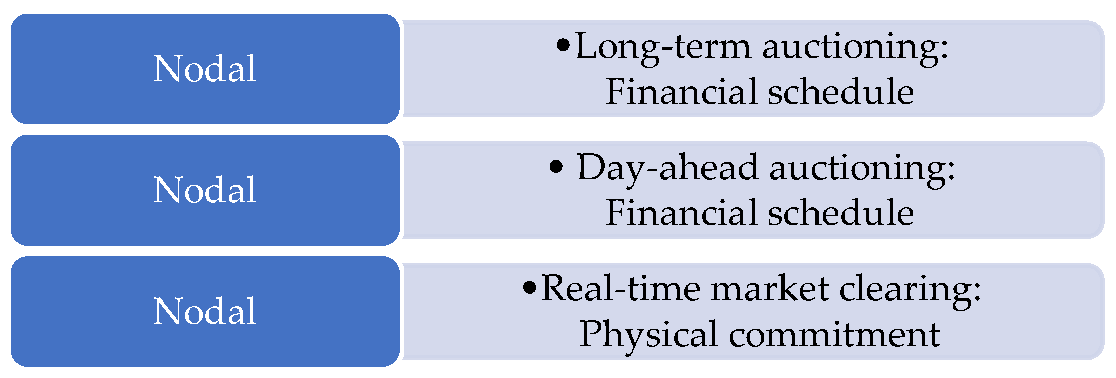
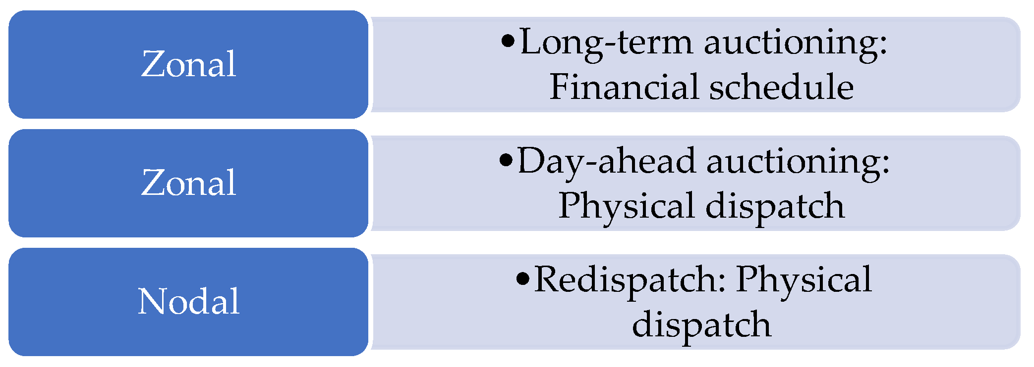
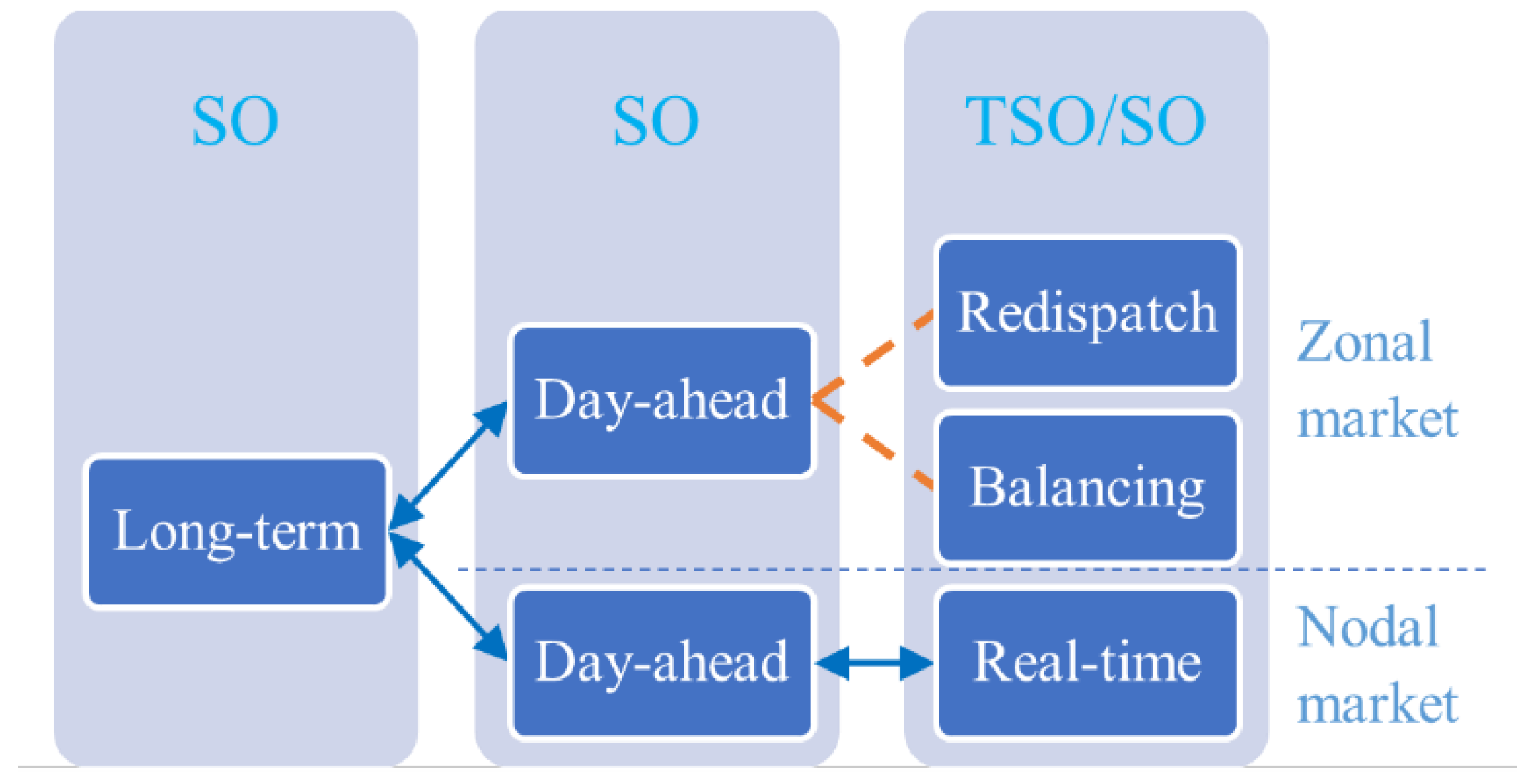
3. Institutions, Spatial, and Temporal Dimensions of Nodal and Zonal Markets

In this section, we discuss how institutions and market rules are structured for the implementation of JETRA under nodal and zonal pricing systems. Long-term, cross-border market development necessitates an examination of both the temporal and special dimensions: how market outcomes in different timeframes are connected and how cross-border markets are integrated. The focus of this study is the effectiveness of long-term market hedging instruments. However, the long-term market is not only about the long-term, since the payback of hedging instruments is based on the spot market outcome. Therefore, the long-term market needs to be linked with the short-term market in a compatible manner.
Section 3.1 presents the institutional settings for JETRA implementation. While JETRA under nodal pricing follows the Independent System Operator (ISO) model, the long-term market under zonal pricing follows the day-ahead market coupling institutional settings. In contrast to the European TSO model where network operator and owner are the same entity, the ISO model in the U.S. context refers to system operators who are asset light and oversee both market and network operations. In Section 3.2, the spatial and temporal aspects of JETRA implementation under different market structures are examined and compared. This section also explains how multi-settlement rules link various market timeframes and how their application is determined by the nature of market clearing, whether they are physical commitments for dispatch or financial schedules.

3.1. Institutional Design

As noted by O’Neill, the ISO, tasked with managing both the market and network operations, is in an advantageous position for conducting JETRA. This institution arrangement can allow optimization to incorporate network constraints, generation, load, and the net import or export of each node [25]. Therefore, under the nodal pricing framework in this research, an ISO that optimizes market and network operations simultaneously administers JETRA.
The day-ahead market serves as the backbone of the European internal electricity market [26]. The selected mechanism for day-ahead market coupling has a profound influence on the institutional role of the European cross-border electricity market. The FBMC, currently implemented in a day-ahead timeframe, aligns with a decentralized market structure. In this structure, power exchange and TSO at the national level interact to clear the market.
Under zonal pricing, the JETRA follows institutional designs that revolve around the current European day-ahead market. The long-term and day-ahead auctions are cleared by power exchanges, with zonal grid model input from the TSOs. SOs at this stage are power exchanges or TSOs. After the gate closure of the spot market, redispatch and balancing are the sole responsibility of the TSOs, who manage the grid and act as single buyers in the market. Thus, TSOs are in a better position to make settlements at this stage. After market closure, the term “SO” in the timeframe refers only to TSOs.

3.2. Financial Schedule and Physical Dispatch

The determination of dispatch as either a financial schedule or physical commitment can fundamentally shape how multi-settlement rules interconnect various market timeframes. A long-term auction is designed to have a financial schedule, as the main objective is to provide hedging opportunities with a financial position over a long-term timeframe. Aligned with the market conventions established by some U.S. ISOs, day-ahead and real-time operations are financial dispatch and physical dispatch, respectively.
Energy and transmission rights obtained from the forward market, which are financial contracts, will be liquidated in subsequent auction rounds. Consequently, these financial schedules are not directly linked to actual energy delivery or the use of the transmission network in real-time operation. Only the real-time market entails physical dispatch, where bidders must adhere to the SO’s instructions or face financial penalties [22]. In the real-time market, generation capability, demand level, and bilateral contracts are factored in as constraints under the JETRA model [16].
A consistent nodal grid model is employed across all three timeframes. For each bid, a separate nodal PTDF is applied in the grid modeling under the original nodal pricing design. Figure 2 illustrates the temporal and spatial dimensions of JETRA under nodal pricing.
In the simplified case study, which elucidates market logic, the long-term market is directly linked to the day-ahead market and is followed by post-spot market arrangements. Accepted bids for FTRs, PTRs, and forward energy contracts in the long-term market constitute financial schedules. In the day-ahead market coupling, all previously procured rights and energy contracts are liquidated. Right holders are paid or required to pay for the product of the quantity awarded in a long-term auction, with prices determined at the day-ahead market clearing.
Adhering to the current market rule, the day-ahead market produces physical schedules. The sequential allocation of network capacity is implemented from the day-ahead market onwards, and capacity allocation has physical commitment. This suggests that market schedules from the day-ahead market onwards cannot be liquidated by the SO and that multi-settlement rules cannot connect timeframes after the day-ahead market. Long-term energy and transmission rights settled at day-ahead market prices do not cover costs incurred after the day-ahead market gate closure.
After gate closure, the SO assesses the feasibility of day-ahead market clearing outcomes by calculating the load flows of the whole system. If the estimated power flow exceeds the network capacity limit, then the SO can adjust the scheduled generation or load pattern from the day-ahead market to alleviate congestion. Some generators in certain locations that have not been scheduled in the market coupling due to higher costs that exceed the market clearing price, are required to be dispatched. Conversely, some generators that have been scheduled for production in the day-ahead market are asked to reduce their output. When the physical schedule is changed in the redispatch phase, pre-negotiated rules are required to allocate the additional costs incurred either as payment for dispatched-up generation or as compensation for foregone revenues for dispatched-down generators. Figure 3 illustrates the temporal and spatial dimensions of JETRA under zonal pricing.
As explained in detail in Section 4 and demonstrated in Section 5, grid modeling for both long-term and day-ahead markets incorporates the zonal grid model into the optimization process. In the redispatch stage, system cost optimization is executed by TSOs while considering transmission network constraints through a nodal grid view.
Figure 4 summarizes the market timeframes, institutions, and the multi-settlement rule application range, with zonal pricing at the top and nodal pricing at the bottom. Lines with arrows indicate the auctions interconnected by the multi-settlement rules of the JETRA. The SO under nodal pricing implies that the ISO is responsible for auctions in all timeframes, while the SO in long-term and day-ahead timeframes under zonal pricing can be the TSO or power exchange.
The lower section of Figure 4 depicts the markets in the case study connected by multi-settlement rules under nodal pricing, namely long-term, day-ahead, and real-time markets. This has crucial implications for how the hedging functions and the total cost index are computed later in Section 6. For instance, in the multi-settlement rule example in Section 2.2, the market participant has 100 MWh bilateral long-term contracts, bids a 100 MWh FTR that corresponds to its contractual locations, and has the bids accepted at €5/MWh in the long-term auction. It can continue to bid 100 MWh in the day-ahead and real-time markets at any cost and eventually be paid back at the real-time price. Therefore, the real-time congestion price risk for its 100 MWh bilateral contract is hedged with a total cost of €500 paid at the long-term auction.
The upper section of Figure 4 demonstrates that the multi-settlement rules link the long-term and day-ahead auctions under zonal pricing. The dashed lines indicate that multi-settlement rules do not apply in the timeframe after the day-ahead market closure. In the above example, since the day-ahead market is the last round of the joint auction, the market participant will be paid back at the day-ahead market price. In the redispatch phase, if additional costs are incurred to ensure grid feasibility, this market participant may be allocated redispatch costs. In contrast to nodal pricing, there are no market instruments for the market player to procure to hedge against the redispatch costs, which are essentially incurred to alleviate system congestion after the market closure. Therefore, the redispatch costs allocated to the market player become an additional cost component in the total costs paid by the market players.
The institutional arrangements discussed in this section play a crucial role in the grid modeling process in Section 4. Meanwhile, the financial and physical rules as well as the application of multi-settlement rules have important implications for JETRA implementation results, such as the total costs for market players across different timeframes, as Section 6 demonstrates.

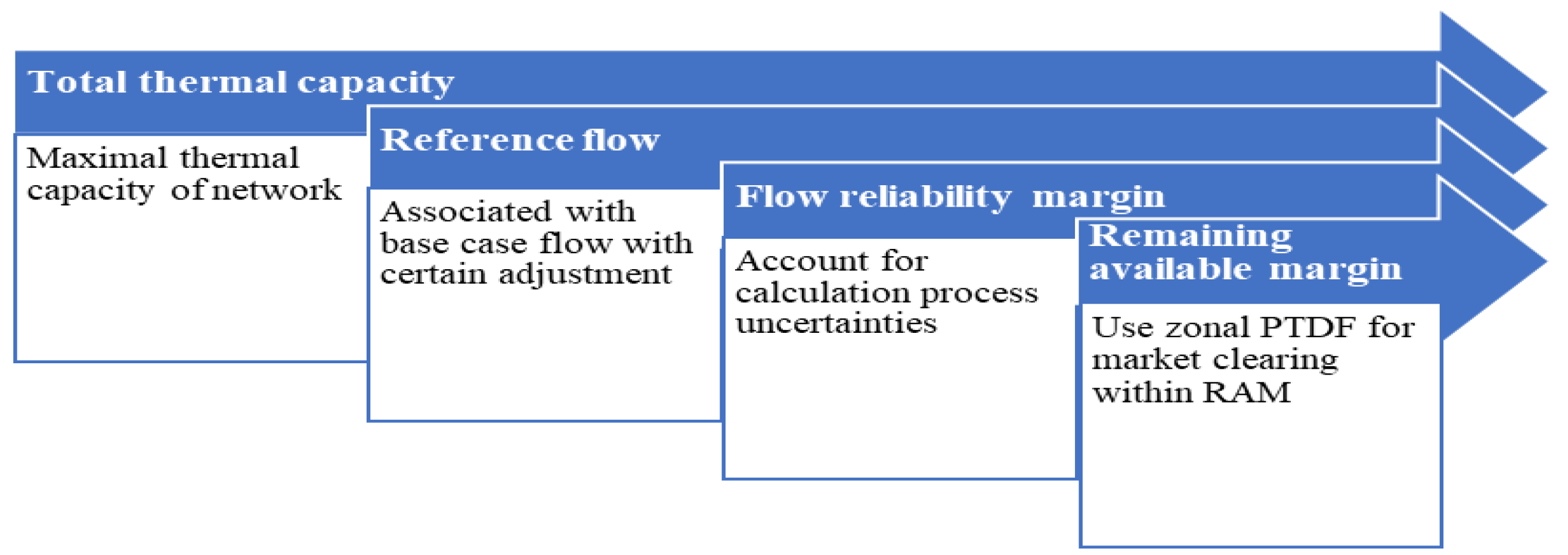
4. Adapting JETRA to Flow-Based Market Coupling

In this section, we discuss grid modeling of JETRA implementation under zonal pricing with the FBMC methodology. Section 4.1 first introduces the FBMC mechanism, proposes the institutional function and computation process for JETRA implementation adapted to FBMC, and analyses what constitutes a good set of grid modeling parameters for FBMC.
In Section 4.2, Section 4.2.1 first discusses an important grid modeling requirement for JETRA under zonal pricing, namely the need to guarantee the firmness of cross-border FTRs. It then summarizes the information asymmetry between the SO and market players for zonal pricing market clearing and introduces the flow reliability margin (FRM) to address uncertainties associated with the information asymmetries.
Next, Section 4.2.2 and Section 4.2.3 explain why JETRA under FBMC imposes greater challenges for either realistic base case construction or interzonal PTDF estimation compared with the currently implemented day-ahead market coupling. Lastly, Section 4.3 explains the challenges of day-ahead auction grid modeling, the proposed rule for addressing the problems, and the two redispatch methods adopted in this research.

4.1. Flow-Based Market Coupling

4.1.1. JETRA with Flow-Based Market Coupling

The auction objective of JETRA adapted to FBMC is to maximize bid values while respecting energy supply and demand equilibrium and interconnection flow limits. Shadow prices are calculated as dual variables of the interzonal line flow constraint. The dual variable from the energy balance equation gives the hub zone price, which is the demand zone in the case study. Similar to nodal pricing, under FBMC, interconnection capacity allocation and interzonal transactions are simultaneously determined. Unlike nodal pricing, a simplified zonal network model is computed by TSOs as a result of the forecast for market clearing. All sellers within a bidding zone receive the same zonal price, and all buyers pay the same.
The network flow estimation is segmented into two main parts in the currently implemented FBMC. The main components of the interconnection capacity are depicted in Figure 5. The first part is the reference flow associated with the base case, which represents the best estimate of the system state on the operating day. The second part is the flow because of the zonal net position deviation between the day-ahead market operating point and the base case. The remaining available margin (RAM) refers to the available capacity on the critical branches for the amount of net position change between the day-ahead market coupling outcome and the base case. When calculating the RAM, an FRM is deducted from the total thermal capacity to account for calculation process uncertainties.
To close the gap between the day-ahead market operating point and the base case, a set of generators with a predetermined share of output change are assumed to react to the zonal net position changes [27]. The GSKs are thus defined as the nodal change of the generation output in relation to the zonal net position variation. The zonal PTDF represents the distribution of power flow on the cross-border network elements from a unit change in net injection or withdrawal in the specified zone.
Table 2 summarizes the real-world process for TSOs and power exchanges at different timeframes as well as the computation process in JETRA under zonal pricing for the case study. Centered around the FBMC methodology, the role of TSOs and power exchanges in the long-term auction follows that of the day-ahead market.

4.1.2. Base Case and Zonal PTDF

The zonal PTDF and base case are critical grid modeling inputs for market clearing. With zero interzonal trade, lines can still be loaded with energy trade occurring within a bidding zone. Felten et al. highlighted that the main purpose of the base case is to describe the intrazonal trade impact on line loading [24]. Combined with the reasons explained in Section 4.2.1 for JETRA implementation, the base case is used in this research to take only the intrazonal trade and the induced interconnection flow into consideration (i.e., at the equilibrium point with a zero interzonal trade level).
To assess whether JETRA grid modeling based on the flow-based method can result in efficient grid modeling, the first question that we attempt to answer is as follows: What constitutes good grid modeling parameters? The case studies in Appendix B investigate the impact of zonal PTDF and base case selection on interconnection flow estimation under FBMC.
  • The base case plays a crucial role in defining the feasible region for interzonal trade volume, and its construction provides another source of flow estimation error. As case A in Appendix B shows, neglecting intrazonal network constraints in the zonal market model can result in a much higher cleared volume of intrazonal transactions compared with nodal dispatch. This high intrazonal trade not only results in intrazonal congestion but also leads to an initial underestimation of the impact of intrazonal trade on interconnection capacity utilization in grid modeling. Consequently, it results in an overoptimistic, feasible flow region for potential interzonal trade at the grid modeling stage.
  • An overly stringent zonal PTDF can lead to the overestimation of interconnection flow, and the zonal market clearing outcome can result in the underutilization of interconnection capacity, as in case study C. Meanwhile, overly loose assumptions with smaller than actual zonal PTDF values can lead to an underestimation of interconnection flow in the grid modeling process. As a result, zonal market clearing can result in interconnection congestion and require redispatch, as indicated in case B.
To derive a more accurate power flow estimation and interzonal trade domain, we need to combine a realistic base case that represents intrazonal trade and a realistic zonal PTDF value. The realistic grid modeling parameters should reflect intrazonal trade and interzonal injection/withdrawal patterns in zonal market clearing. We focus on the methodological comparison of JETRA under nodal and zonal pricing so that the stochastic nature of transmission capacity, which is present under nodal and zonal pricing in the long-term auction, is not modelled in the case study. The same total network capacities of critical branches are assumed in the long-term and short-term auctions in this research to focus on the role of uncertainties caused by information asymmetry. After discussing what constitutes good grid modeling parameters, we analyse in Section 4.2 why JETRA’s adaptation to FBMC presents challenges in accurately determining these parameters, particularly in the long-term auction.

4.2. JETEA Adaptation to Flow-Based Market Coupling: Methodological Challenges

4.2.1. FTR Firmness under High Uncertainty

In the JETRA framework under nodal pricing, the firmness of FTRs and overall flow feasibility are guaranteed by the load flow constraints within each auction round. FTRs, representing the forward sale of network capacity, are allocated alongside energy and PTRs through an optimization process that considers the nodal view of the network. The rules governing PTDFs and network capacity limits across different auction rounds ensure the physical feasibility of accepted energy and transmission right bids in subsequent rounds, as demonstrated in Appendix C.
Conversely, the FBMC for the day-ahead market only allows energy bids. Here, redispatch after market closure can ex-post adjust energy injection withdrawal patterns to ensure grid feasibility. During redispatch, curtailment of electricity supply with energy injection rights from the day-ahead market often occurs, with compensation for foregone revenue. In typical redispatch scenarios without load shedding, energy withdrawal rights are respected, while energy injection rights are financially compensated, and the physical dispatch of accepted bids from short-term markets is not always guaranteed.
A crucial requirement for zonal grid modeling in JETRA implementation is the firmness of the energy injection and withdrawal rights. The PTR impact on the interconnection capacity does not need to go through zonal PTDF multiplication by the SO in the grid modeling stage as that for FTR, although market players may still need the zonal PTDF values to compose their PTR portfolios. This can be seen as the PTDF values for PTR bids in the specified transmission link are set to 1 by the SO. The physical feasibility of accepted PTR bids can be ensured directly by the transmission capacity constraints. The assumption in this research is that the market players who seek energy bids in the forward markets use them to hedge against price volatility in the subsequent auctions until the day-ahead market as the physical dispatch. In this context, their expectations regarding redispatch are assumed to align with those of the day-ahead energy bidders.
A key distinction between cross-border FTRs and the energy bids lies in the FTR specification of volume and location of both energy injection and withdrawal points for the bilateral transactions. In contrast, energy bids only specify the volume of energy to be injected or withdrawn separately at specific points and can be used to match load or generation across the whole system. Therefore, energy transactions in FTRs are assigned a specific direction (e.g., from zone A to zone B). The specification of both injection and withdrawal points in FTR bids reveals whether they are used for cross-border trade.
In some U.S. systems, FTR allocation must undergo a simultaneous feasibility test, which is essentially an optimization algorithm. When the FTRs are the result of the optimization process that adheres to the transmission constraints, they are simultaneously feasible [28]. In the context of this research, the zonal system’s aggregated zones correspond to nodes in the nodal system, while the cross-border transmission network functions as the elements linking these zones. D’Aertrycke and Smeers emphasize the need for long-term FTRs allocated in the European zonal system to be physically feasible within the day-ahead market [9].
As FTRs represent forward sales of transmission capacity, we argue that market players who purchase cross-border FTRs to support their bilateral contracts should not incur additional redispatch for cross-border transmission services. Otherwise, the effectiveness of FTRs as hedging instruments against cross-border congestion risk within joint auctions will be weakened. In this research, we require the cross-zonal FTRs to be physically feasible in each auction round. In other words, the interconnection flow resulting from the allocated FTRs should not breach the transmission capacity limit used in auction optimization. The equations presented in Appendix C demonstrate that cross-border FTRs that are physically feasible in preceding auctions remain firm in subsequent auctions, assuming no changes in grid typology. Consequently, the FTRs allocated in the JETRA long-term auction will also be feasible in the day-ahead market.
Compared to the current day-ahead FBMC, cross-border FTR bids that specify the energy injection and withdrawal locations for specific transactions pose a greater challenge to grid modeling by TSOs. This increased complexity arises from several key differences between the two approaches.
  • Day-ahead FBMC: As the European day-ahead market reflects physical dispatch that corresponds to generation and load patterns, TSOs can leverage historical operating data to approximate the physical flow resulting from market clearing. Additionally, TSOs retain the option to utilize the redispatch mechanism to adjust the day-ahead market energy bids, ensuring grid feasibility.
  • JETRA with FTRs: The financial forwards in JETRA long-term auctions may not correspond directly with the overall generation and load patterns within physical dispatch. For instance, FTRs are part of a bidding portfolio spanning long-term and short-term markets. Forecasting market participant bidding behavior and assessing their impact on interconnection flow is significantly more challenging compared to forecasting generation load patterns before the short-term market. Section 4.2.2 will illustrate with an example why the base case method used in day-ahead FBMC is not applicable when both the energy and FTR bids are involved in the long-term market. Additionally, to uphold the integrity of the long-term contracts supported by FTRs, redispatch cannot curtail the generation specified as energy injection within cross-border FTRs. To guarantee the physical feasibility of long-term JETRA bids, an additional GDSK rule is proposed in Section 4.2.3 proposes an additional GDSK rule, and a higher FRM is applied in the grid modeling of long-term auctions.
In the original JETRA design under zonal pricing, the use of separate PTDF values is applied for each energy purchase or sale and the FTR bid in the network flow constraint calculation. In the nodal pricing market, the SO does not need to know the financial hedging strategy or long-term contracts of market players for market clearing. The SO can clear the market on the basis of bids and estimated network conditions.
As part of the FBMC, a grid model with interzonal PTDF values and RAM is established prior to market opening. This requires TSOs to forecast energy injection/withdrawal patterns as well as physical flows, which are related to bidding information about energy sale/purchase or FTR bid volume and the exact locations. In JETRA, the flexibility for market players to choose across different timeframes from various hedging mechanisms, from energy to transmission right products, and to implement their own investment strategy intensifies the information required for constructing grid models. The intensified information asymmetry between SO and market players makes it extremely difficult, if possible, to determine the ex-ante base case and separate zonal PTDF in the JETRA implementation. In this research, an integrated interzonal PTDF is employed to represent the combined effect of cross-border transactions through energy purchase/sale bids and FTRs on the interconnection flow.
Schönheit et al. explained the reasons for using FRM to address flow estimation errors in FBMC [13]. The parameters involved in FBMC are inherently predictive, which introduces inevitable errors in flow estimation. In this research, FRM is implemented to account for the uncertainties that arise from the information asymmetry between market players and the SO. Its purpose is to ensure the system reliability of JETRA.
Because of the significant uncertainties associated with base case construction and PTDF determination in the long-term auction of JETRA, a higher FRM is employed to compensate for flow estimation errors. However, a high FRM value also imposes restrictions on the feasible region for interzonal trade.

4.2.2. Base Case Effectiveness in a Long-Term Auction

The currently implemented base case uses a snapshot of the power system on a selected reference day. It then updates the net positions of each zone by considering the forecasted levels of renewable generation and load for the operation day. Subsequently, base cases from different TSOs are merged, with an agreement on exchange programs [29]. The reference flow represents the physical flow of the common base case, considering the exchange programs from the selected reference day. As the day-ahead market dispatch is physical in nature, the base case approach corresponds to the actual energy injection and withdrawal patterns. Voswinkel et al. noted that the uncertainties associated with the expected net positions in the base case construction are linked to the forecast errors of intermittent energy sources, variations in load, and unexpected plant outages [30].
Moreover, the combination of the base case and the GSK metric assumes that the small net position gap between the base case and the operation point can be served by anticipating a set of generators with a predetermined output change ratio [27]. However, the effectiveness of these assumptions is called into question in the context of the JETRA long-term auction.
Unlike the day-ahead market, the generation load pattern in a long-term auction may undergo structural changes due to generation investments, retirements, or load shifting. Additionally, the flexibility in choosing hedging products in JETRA, as well as hedging across different market timeframes, means that the bids in JETRA and the auction clearing outcome do not always align with the physical energy injection or withdrawal on an operation day. The combination of products and strategies across different timeframes for market players makes it challenging for TSOs to construct a reasonable base case based on previous auction outcomes or the operation point from historical data.
Similar to the current approach used in day-ahead market coupling, we can examine the bidding information available from previous rounds of long-term joint auctions, which occur weeks or months before the current auction round. For instance, given the assumption that TSOs can estimate where the energy purchase bids are located well based on operational experience, it is conceivable that a notable difference exists in the accumulated energy purchase in zone east in the last auction compared with its current demand level at node 3 as the main load center. The energy purchase bid in zone east accounts for 250 MWh trade in the last round of the long-term auction, while the current demand level is around 500 MWh. This observation suggests the possibility of significantly less accumulated energy purchased at node 3 in the previous auction. Several scenarios could explain this phenomenon, which are described as follows:
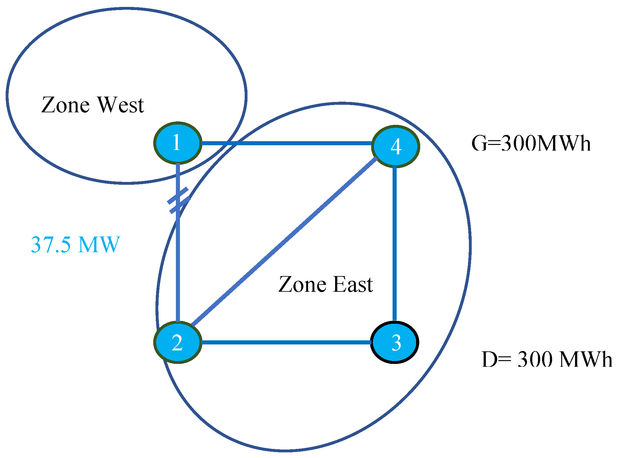
  • Scenario 1: In a forward market auction, the energy purchase quantity solely represents the total amount of energy bid into hedging products from the demand side, which may not necessarily align with the expected real-time load. It is possible that the main demand at node 3 adopts a strategy of spreading out energy bids across different timeframes, resulting in a lower energy purchase bid in the long-term auction. In other words, the demand at node 3 may employ a bidding strategy to acquire a portion of its load in later market frames, anticipating a potential decrease in spot market prices.
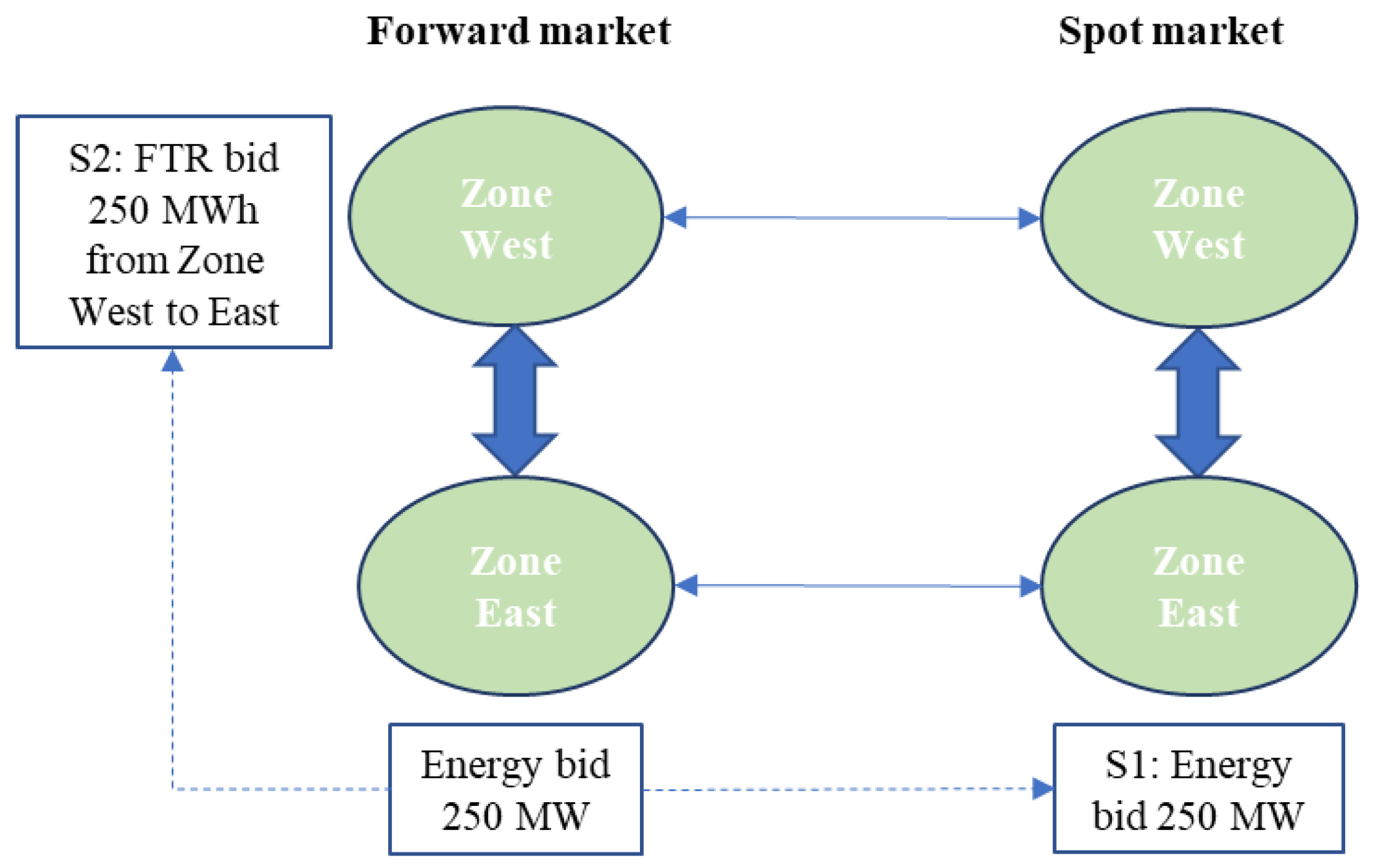
  • Scenario 2: Another possibility is that the demand at load 3 enters into a long-term, cross-border bilateral contract to fulfill a significant portion of its future energy demand, while the supplier in zone west submits FTR bids to support these long-term contracts. Considering the lead time in the long-term market, generation sources involved from zone west could potentially include new power plants that have not yet reached the operational phase. Consequently, the base case, which relies on historical data, may not accurately capture the transactions associated with these new investments. Moreover, in the joint auction, only injection/withdrawal zone information is available for the FTR bids, which limits the ability of TSOs to effectively forecast the demand pattern solely based on the observed results of the previous auction round. Scenarios 1 and 2 are illustrated in Figure 6 with textboxes S1 and S2:
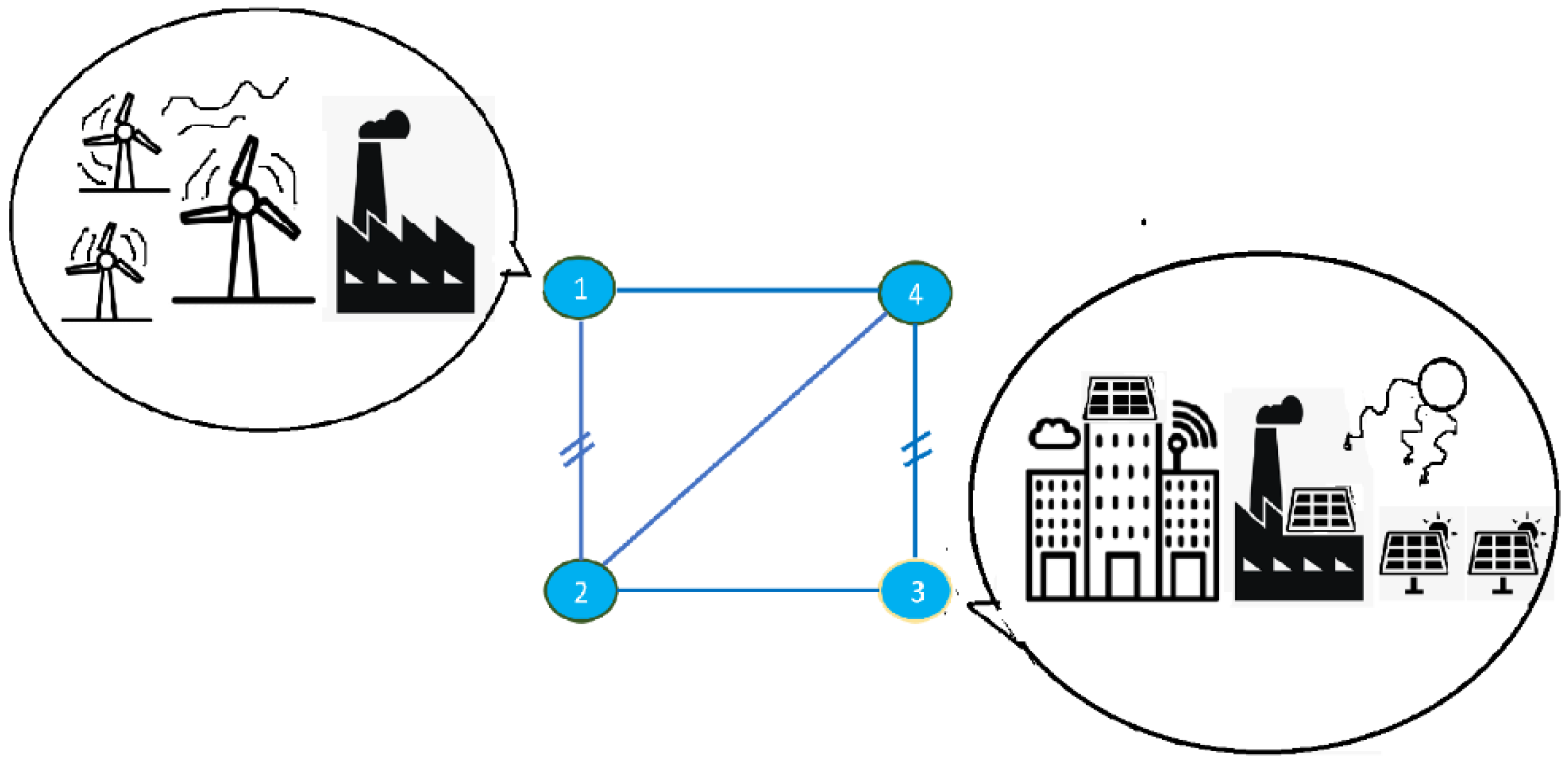
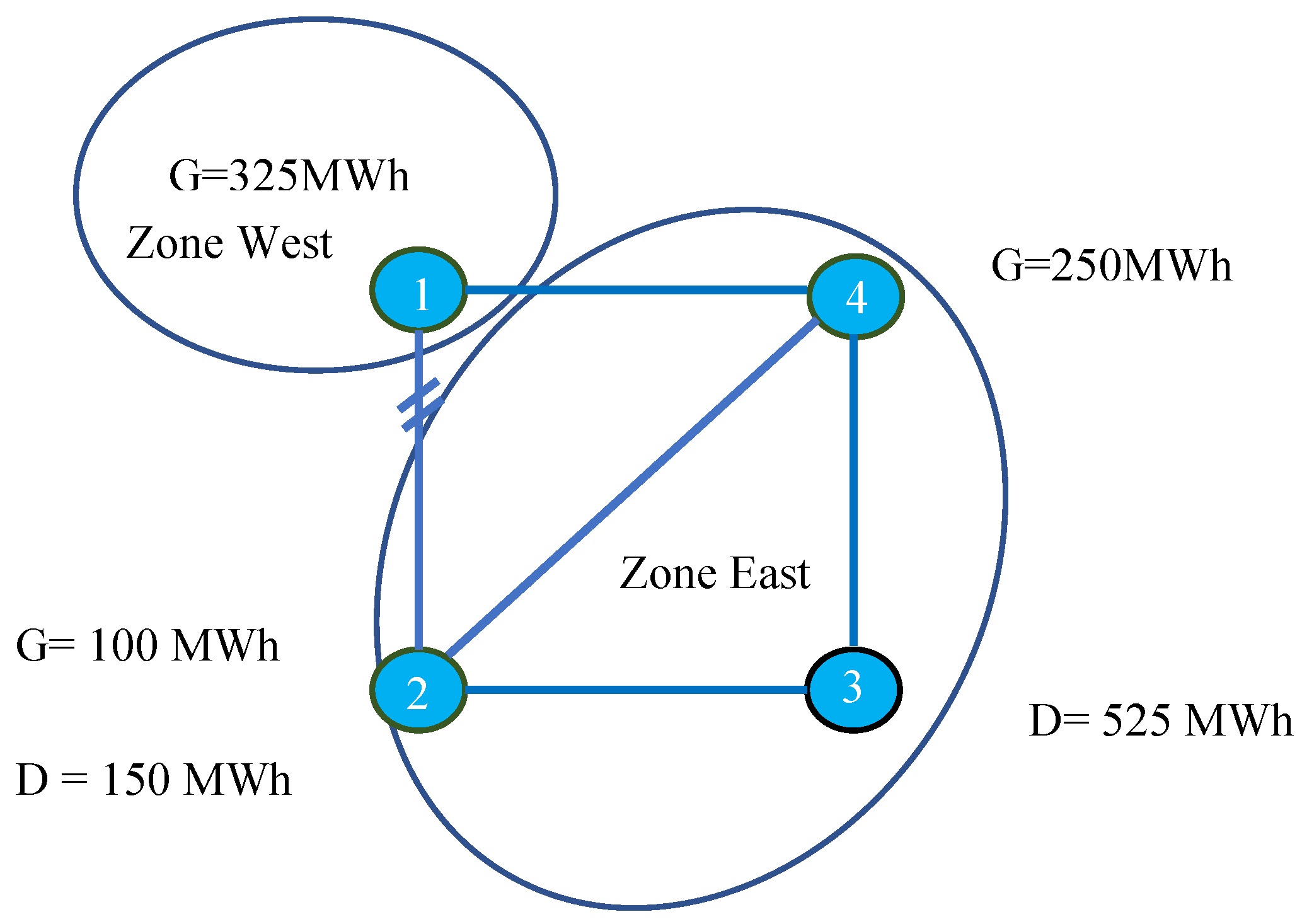
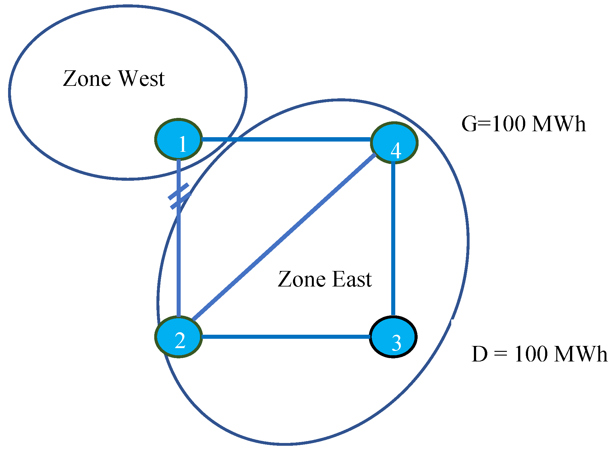
  • Scenario 3: Considering the lead time before electricity delivery, whether the lower energy bid volume in zone east is the result of planned structural changes on the demand side is worth questioning. One possible explanation is that there is a planned demand shift at node 3, which is achieved by relocating industries closer to low-cost renewable energy sources at node 1 as illustrated in the left circle of Figure 7. This strategy could decrease energy purchase bids from the main load center during the long-term auction.
  • Scenario 4: Another scenario to consider is a net reduction in demand resulting from investments in local generation, as illustrated in the right circle of Figure 7. This example highlights the limitations of relying on reference day generation and load bid profiles from historical data for long-term auctions.
This example demonstrates that market bidding behavior, generational investment decisions, and evolving demand patterns in the long term make the historical data approach that is currently implemented for base case construction less applicable. Therefore, the base case used in this research approximates the impact of intrazonal transactions on interconnection flow at the zero net import/export level. The base case derived for the long-term and day-ahead auctions is presented in Section 5.2. A reference day generation load pattern, after redispatch, is used to consider the overall flow on the interconnection. The load flow that results from the interzonal power exchange is subtracted from the total to account for the intrazonal transaction impact on the interconnection.

4.2.3. GDSK Rule for Conservative Grid Modeling

Smeers highlighted that the construction of zone-to-line PTDFs in FBMC relies on the assumption that TSOs can accurately estimate the day-ahead market outcome flows during grid modeling [18]. This assumption is based on the notion that the energy injection and withdrawal patterns following market clearing do not differ significantly from one working day to another or from a weekend day to the corresponding day of the previous weekend. The energy injection and withdrawal pattern in the chosen base case may be close to that of the operation day. Furthermore, the part of energy injection patterns in reaction to zonal net position change, reflected in the weights of the GSK metric, is more likely to be close to the realized energy generation patterns after the market clears. Under these circumstances, zone-to-line PTDFs provide a good representation of the grid. However, this assumption is not applicable in the forward market, and zonal PTDFs are subject to additional requirements in JETRA under zonal pricing to ensure the firmness of cross-border FTRs.
As discussed in the previous section, information asymmetry between the SO and market players poses a significant challenge for long-term auction grid modeling. By using a single set of PTDFs for interzonal transactions, we assume that energy and FTRs follow the same injection and withdrawal patterns at the aggregated level.
In Section 4.2.1, we have discussed the firmness requirement of cross-border FTRs under zonal pricing in each auction round. Implementing a single set of zonal PTDFs also implies that all cross-border transactions for grid modeling must adhere to the firmness requirements of cross-border FTRs.
To ensure the feasibility of interconnection flow in the long-term auction, we propose two rules for the GDSK in the import region:
  • Using dispatchable generators,
  • Assigning a higher weight to the generation decrease or demand increase at the node associated with the critical transaction from a congestion perspective for interconnection lines.
Rule 1 aligns with the currently implemented FBMC approach, which ensures reliable system operation. Rule 2, introduced in this research, is inspired by and adjusted from the worst-case analysis approach of D’Aertrycke and Smeers to ensure the feasibility of interconnection flow for FTRs under the TC model [9,31]. A single set of zonal PTDF can be seen as a weighted sum of nodal PTDF, with weights assigned by the GDSK. Therefore, a GDSK metric that assigns a higher weight to critical nodes associated with a higher PTDF value in Rule 2 implies that the assumed energy trade pattern in grid modeling includes a greater proportion of interzonal trade coming from nodes linked to critical trade patterns.
The rationale for assigning a higher GDSK weight to the withdrawal node associated with the most critical cross-border transaction pattern can be illustrated through the following simple example: If the corresponding TSO in the case study assumes that the cross-border FTR withdrawal point in zone east is at node 3, then the zonal PTDF will be 0.5. The maximum allowed transaction will be 400 MW from zone west to zone east. However, if the actual FTR withdrawal point is node 2, then the zonal PTDF will be 0.625, while the maximum allowed transaction will be 320 MW. Consequently, the FTRs allocated in the auction clearing between 320 and 400 MW from zone west to zone east cannot be considered firm.
The scenarios analyzed in Section 4.2.2 regarding the base case imply that the volume and location of energy withdrawal are subject to uncertainties in zone east. Consequently, unlike the day-ahead market, a forward market forecast should encompass a more diverse range of energy transaction patterns to cover a vast array of possibilities. Market uncertainties are translated into more conservative grid modeling to ensure FTR firmness. When nodes with higher PTDF on the interconnection line are designated as import nodes with a higher GDSK weight, higher interconnection flow volumes can be assumed by the market model compared with nodes with lower PTDF on the interconnection. However, this GDSK rule may result in stringent zonal PTDFs and impose more restrictions on interconnection capacity utilization. The application of GDSK rules in the case study is demonstrated in Section 5.2.3. The inefficiency of implementing a single zonal PTDF and the proposed GDSK rule, compared with nodal pricing, is assessed by the Euclidean distances between GDSK metrics in Section 6.2.

4.3. Grid Modeling for JETRA in the Day-Ahead Market and Redispatch

The day-ahead market in Europe under zonal pricing is treated as the real-time market under nodal pricing because both involve physical dispatch. Under nodal pricing, bilateral trade is made binding by setting the lower and upper boundaries of the FTR bid backing the bilateral contract in the real-time market [16]. Under current market rules, the exact nodal positions of bidders are not known to the SO at the time of market clearing. Moreover, there is no nodal representation in the zonal network to apply in which the FTR bid can be specified with an injection or withdrawal location. Similar to the approach in a long-term timeframe, we make bilateral contracts backed up by cross-border transmission rights physically feasible by constructing a more conservative grid model in the day-ahead market. Meanwhile, the GDSK rules used in the day-ahead market are relaxed to ensure that the interzonal PTDF in the day-ahead timeframe is smaller than that of the long-term auction, as required by the JETRA revenue adequacy rule discussed in Section 2.
After the day-ahead market closure, the case studies proceed directly to the redispatch phase. After gate closure, the SO assesses the feasibility of day-ahead market clearing outcomes by calculating load flows on the whole system. When the estimated power flow exceeds the network capacity limit, the SO can alter the scheduled generation or load pattern from the day-ahead market to relieve congestion. Some generators in certain locations have not been scheduled in the market coupling because their costs are higher than the market clearing price, and they are required to be dispatched, while some generators have been scheduled to produce in the day-ahead market, and they are required to reduce their production.
Redispatch costs add to the accumulated costs for final consumers under zonal pricing. In recent years, with increased renewable integration, redispatch costs have risen sharply for European TSOs [32]. Redispatch cost allocation according to the requester-pays principle has stirred controversy in Europe [33]. The choice of methods according to the polluter-pays principle is also subject to disputes among European TSOs [34].
An interesting comparison for this study is the need for redispatch cost distribution under nodal and zonal pricing. Because all network capacity constraints are included in the optimization of different auctioning timeframes, there is no need for redispatch under nodal pricing. In each phase of the market, the generation and load net payments are sufficient for the SO to pay the bid winners from the previous auction. Under zonal pricing, the case study demonstrates that simplified network representation necessitates redispatch to correct the generation load patterns. The redispatch process, which occurs after market closure, raises the need to allocate additional costs across borders according to pre-agreed rules. In this study, we also demonstrate that different redispatch mechanisms have an impact on redispatch costs, following Oggio et al. and Kunz et al. [35,36]. The variation in redispatch costs thus influences the total costs to be allocated across borders outside the market mechanism.
In the case study, we implement two redispatch models. The first model follows a national redispatch approach that only allows TSOs to use the resources within their bidding zone to alleviate internal network congestion. In this case, the interconnection capacity remains unchanged from the day-ahead market clearing. Furthermore, only the intrazonal network capacity limit is imposed as the constraint for altering the generation load patterns. The second model implements a deeply integrated cross-border redispatch mechanism. Under this approach, the TSOs coordinate as if there is a single SO across borders that can optimize the generation resources and network capacity to minimize the system cost. In addition, the intrazonal constraint is included in the optimization to alleviate congestion on the overloaded lines. Real flow on the interconnection because of the day-ahead schedule is calculated, and the remaining interconnection capacity can be used in the redispatch process. Using the grid modeling rules to adapt JETRA with FBMC discussed in this section, we present its implementation and the results of the case study in Section 5.

5. Case Study Results

This section presents the calculation for JETRA implementation in the case study under nodal and zonal pricing, respectively. In Section 5.1, market clearing and settlements for JETRA implementation under nodal pricing are presented across the long-term, day-ahead, and real-time market timeframes. Section 5.2 first demonstrates the base case computation for the case study in the long-term and day-ahead markets. Following the discussion in Section 4.2, Section 5.2 then provides an example of applying the GDSK rules and FRM to the case study. Section 5.3 presents the zonal pricing market clearing outcomes for JETRA implementation in the case study, covering the long-term, day-ahead markets, and the redispatch phase. The calculations presented in this study were performed using Python 3.9, with the help of packages such as Pyomo, NumPy, and Matplotlib.

5.1. Market Clearing and Settlements in the Case Study under Nodal Pricing

5.1.1. Long-Term Auction Outcome under Nodal Pricing

Table 3 showcases the β values of each bid from the 3rd to the 7th column, using node 3 as the hub node. In the nodal pricing market, the information from each bid and its corresponding nodal PTDF are used to clear the market. The β values and line capacities are provided in the positive and negative directions. In the case study, node 3 always serves as the hub node; therefore, the PTDF value of the energy purchase or sale bid at node 3 on any transmission link is 0. The β values associated with bid 1 are presented in the 3rd column of Table 3. Bid 1 denotes the FTRs between node 1 and node 3. A unit of FTR translates to an injection of 1 MWh at node 1 and a withdrawal at node 3, causing 0.5 MW of power to flow first through line 1–2, and then through line 2–3. Another 0.5 MW of power follows the path from line 1–4 to line 4–3. The PTDF values on lines 1–2, line 2–3, line 1–4, and line 4–3 are 0.5, while the negative directions of the same lines, referred to as lines 2–1, line 3–2, line 4–1, and line 3–4, exhibit PTDF values of −0.5.
Using the bid information in Table 1 and the PTDF values in Table 3, the long-term auction outcome is illustrated in Figure 8. The shadow prices for lines 1–2 and 4–3 are €15/MW and €5/MW, respectively. From the optimization-derived shadow prices, we can infer that lines 1–2 and 4–3 reach their capacity limits. The locational marginal price at hub node 3, which is the dual of the energy balance equation, equals €25/MWh.
The FTR price for bid 1, which accounts for the nodal price difference between nodes 1 and 3, is €10/MWh. Accepted bid volume and prices are shown in the 6th and 7th rows of Table 4. The payments from the long-term auction bid winners to the system operator (SO) are detailed in the final row of Table 4. Bidder 1 pays €3750 to the SO for the 375 FTR between node 1 and node 3, while bidder 5 pays €2500 to the SO for the rights to purchase 100 MWh of energy. Simultaneously, the SO pays €2000 to bidder 3 for the rights to sell 100 MWh of energy.

5.1.2. Day-Ahead and Real-Time Market Outcomes under Nodal Pricing

Because the same bids are submitted to the day-ahead auction in this case study, the day-ahead clearing outcomes are the same as those of the long-term auction. The bid winners of the day-ahead market auction pay the SO an amount identical to that from the long-term auction round; in turn, they receive the same amount back from the SO as right holders.
The main difference between real-time dispatch and the previous auctions is that the real-time dispatch is physical. Consequently, the real-time dispatch incorporates the 500 MWh load level at node 3 as an optimization constraint. Only energy bids and bilateral transactions are taken into account in the real-time market. We posit that bidder 1, who has secured 375 MWh FTR, will match it with a bilateral transaction of 375 MWh between node 1 and node 3. Therefore, the lower bound for the energy purchase bid at node 3 in the real-time market is set at 375 MWh, while the upper bound remains at 500 MWh (We assume the upper bound of the FTR and energy sale bids in the long-term and day-ahead markets have reflected the generation capacity limits). Bid 4, as a transmission right bid, is not allowed to enter the real-time market. The remaining energy supply bids retain the same values as those submitted in the long-term and day-ahead markets. Since node 3 is the hub node, the PTDF value of energy bid from node 1 is the same as the PTDF value of FTR between node 1 and node 3 indicated in Table 3. The PTDF values of other energy bids also stay the same as those of the long-term auction in Table 3. The real-time market dispatch is illustrated in Figure 9. The generator at node 1 produces 400 MW, while those at nodes 2 and 4 each generate 50 MW. Under this dispatch, both lines 1–2 and 4–3 are congested with respective shadow prices of €70/MW and €170/MW. The LMP at hub node 3 is €135/MW, while that at node 1, node 2, and node 4 is 15 €/MW, €80/MW, and €20/MW, respectively. Lines 1–2 and 4–3 are fully utilized in the long-term, day-ahead, and real-time markets.
In the real-time market, the SO receives €67,500 from the load at node 3 while paying out €6000, €1000, and €4000 to generators at node 1, node 4, and node 2, respectively. This process results in a surplus of €56,500. As shown in Table 5, this surplus is used to remunerate the day-ahead market auction bid winners. The FTR held by bidder 1 is priced at €120/MW. Consequently, bidder 1 receives €45,000 from the SO for the 375 MW of FTR it possesses. Bidder 5, who holds the energy purchase right at node 3, is paid at the nodal price of €135/MW, receiving €13,500 from the SO for the 100 MWh energy purchase right. Bidder 3, who was previously compensated by the SO for the energy sale contract, is now required to make a payment to the SO based on the real-time LMP at node 4. This payment amounts to €2000. Consequently, the total net payment from the SO to the bid winners equals €56,500. The surplus from the load and generation payments matches the SO’s net payment to the bid winners, thereby achieving revenue adequacy for the SO.

5.2. Base Cases, GDSK, and FRM in the Case Study

This subsection begins by demonstrating base case construction for the long-term and day-ahead markets under zonal pricing within the case study. As explained in Section 4.2.2, the base case in this research serves to estimate the impact of intrazonal transactions on interconnection at a net position of zero. To achieve this, we proceed with the following steps: First, the system operating point is taken from the selected reference day. Second, the generation and load patterns are modified from the selected day values by reducing the net exchange positions. Finally, the reference flow is derived by modifying the total flow on the interconnections through the reduction in flows resulting from the net exchange positions. Subsequently, this subsection applies the GDSK and FRM rules discussed in Section 4.2 to the case study.

5.2.1. Base Case and Reference Flow in the Long-Term Auction

Figure 10 depicts the generation load pattern on the reference day for the long-term auction. The load at node 2 is served by self-generation on the reference day. The generator in zone west produces 125 MWh, while no load exists within this zone. In zone east, the generator at node 4 generates 300 MWh, while the demand level at node 3 reaches 425 MWh.
To calculate the pattern of intrazonal transactions at a net zero position, a net import quantity of 125 MWh is deducted from the marginal load at node 3 in zone east, and the result is depicted in Figure 11. The reference flow on interconnections 1–2 resulting from the intrazonal transactions is 37.5 MW.

5.2.2. Base Case and Reference Flow in the Day-Ahead Market

Similar to the long-term auction process, the base case is described using the system operation from a reference day and subtracting the flow attributed to net exchange positions. Figure 12 demonstrates the generation load pattern on the reference day selected for the day-ahead market. As illustrated in Figure 12, the load at node 2 is partially served by its own self-generation. Zone west, without any load, generates 325 MWh. Meanwhile, in zone east, the generator at node 4 generates 250 MWh, while the demand level at node 3 totals 525 MWh.
To calculate the intrazonal transactions at zero net position for the joint auction, a net import of 325 MWh is deducted from the load in zone east. A reduction of 50 MWh of the load at node 2 and a reduction of 275 MWh of the load at node 3 are conducted to derive the base case. As illustrated in Figure 13, the reference flow on interconnections 1–2 resulting from intrazonal transactions amounts to 31.25 MW.
The two base cases presented for the long-term and day-ahead markets are close to the intrazonal trade patterns from the zonal pricing based market clearing outcome in Section 5.3, while the interzonal trade patterns in the reference day deviate from the market clearing outcomes, reflecting the challenges discussed in Section 4.2.2. Real-word uncertainties, as discussed in Section 4.2.2, can lead to underestimation or overestimation of the reference flow derived from the base cases. When the reference flow is underestimated, it could pose reliability challenges for the system. When the reference flow is overestimated, it could lower the interconnection utilization rate. Since the reference flow is predictive in nature, at the time of grid modeling, the SO would not be able to determine whether the computed reference flow is an underestimation or an overestimation compared to the real operating point. Therefore, a FRM is required to mitigate the uncertainties from base case construction.

5.2.3. GDSK and FRM in the Long-Term and Day-Ahead Markets

This subsection details the application of the GDSK rule and FRM for the case study in long-term and day-ahead auctions.
As explained in Section 4.2.3, GDSK is determined by a weighted combination of two factors. In this case study:
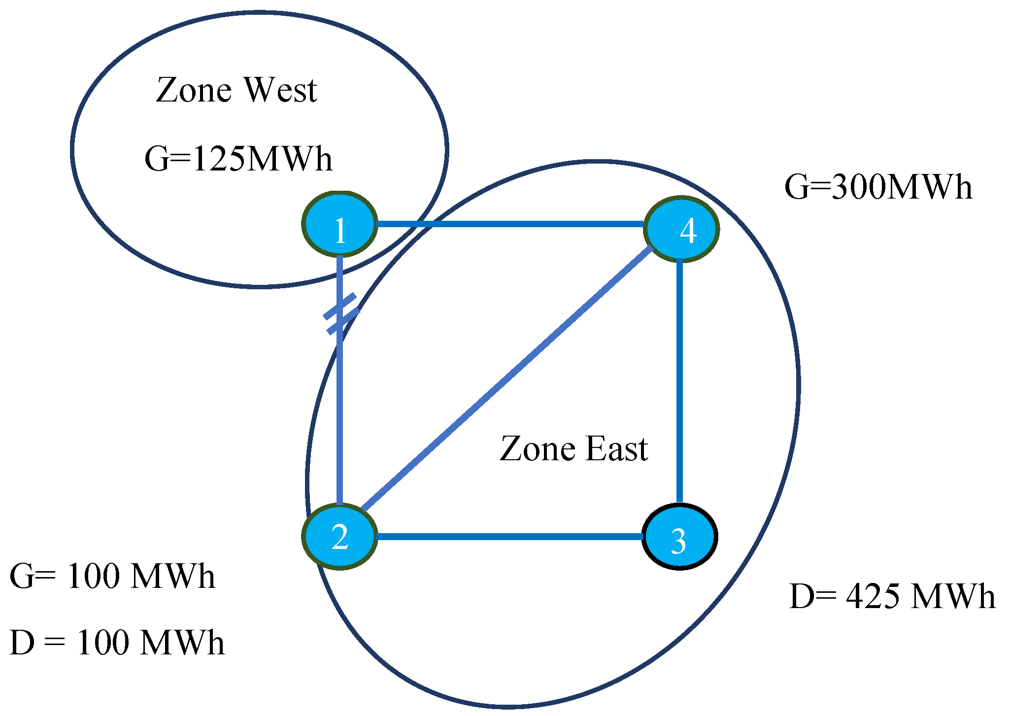
  • Node 4 is characterized as an intermittent generator in zone east with a generation cost that marginally surpasses that of the generator at node 1.
  • The generator at node 2 represents dispatchable generation with a flexible output.
  • The transaction between nodes 1 and 2 exhibits the highest PTDF value on interconnection line 1–2.
Among the generators at nodes 2 and 4, that at node 2 should be selected and given a higher weight according to the GDSK criteria. Imports from zone west can be offset by either an increase in demand or a decrease in generation output in zone east. In the network modeling for long-term auctions, TSOs know from their operational experience that node 3 is the main load center in zone east. However, considering the uncertainties in forecasting long-term transaction patterns, they take the more conservative assumption that a unit export from zone west leads to a 0.5 MW generation decrease at node 2 and a 0.5 MW demand increase at node 3. Therefore, in accordance with rule 2 for GDSK computation discussed in Section 4.2.3, the GDSK between nodes 2, 3, and 4 is set to (0.5, 0.5, 0). The interzonal PTDF on interconnections 1–2 takes the value of 0.5625 in the long-term auction.
The Central Western European (CWE) TSO technical report states that usually 5–20% of maximal capacity is reserved as the FRM for day-ahead market coupling [28]. In the long-term auction, uncertainties regarding the capacity calculation process are higher given the long lead time for generation load forecasts. In this research, the upper value of the FRM range in the day-ahead market coupling is taken as the FRM for interconnections 1–2. The base case selection and reference flow calculation for the long-term auction are presented in Section 5.2.1. With a reference flow of 37.5 MW and FRM of 40 MW, the RAM on interconnections 1–2 is 122.5 MW. The maximal export from zone west to zone east can thus be calculated as 217.8 MW (122.5/0.5625).
As the TSOs receive updated generation and load forecasts closer to the operation day (D-2), they gain more confidence that the majority of imports from zone west will be consumed at node 3. In this case, let us assume that the GDSK for nodes 2, 3, and 4 is set to (0.4, 0.6, 0). With these GDSK weights, the interzonal PTDF value on interconnections 1–2 can be calculated as 0.55 (0.625 × 0.4 + 0.5 × 0.6). For the day-ahead market, a less conservative approach is adopted by selecting the lower value from the FRM range in the CWE region for interconnections 1–2. As detailed in Section 5.2.2, the base case for the day-ahead market establishes a reference flow of 31.25 MW. With this reference flow and FRM of 10 MW, the RAM on interconnections 1–2 becomes 158.75 MW.

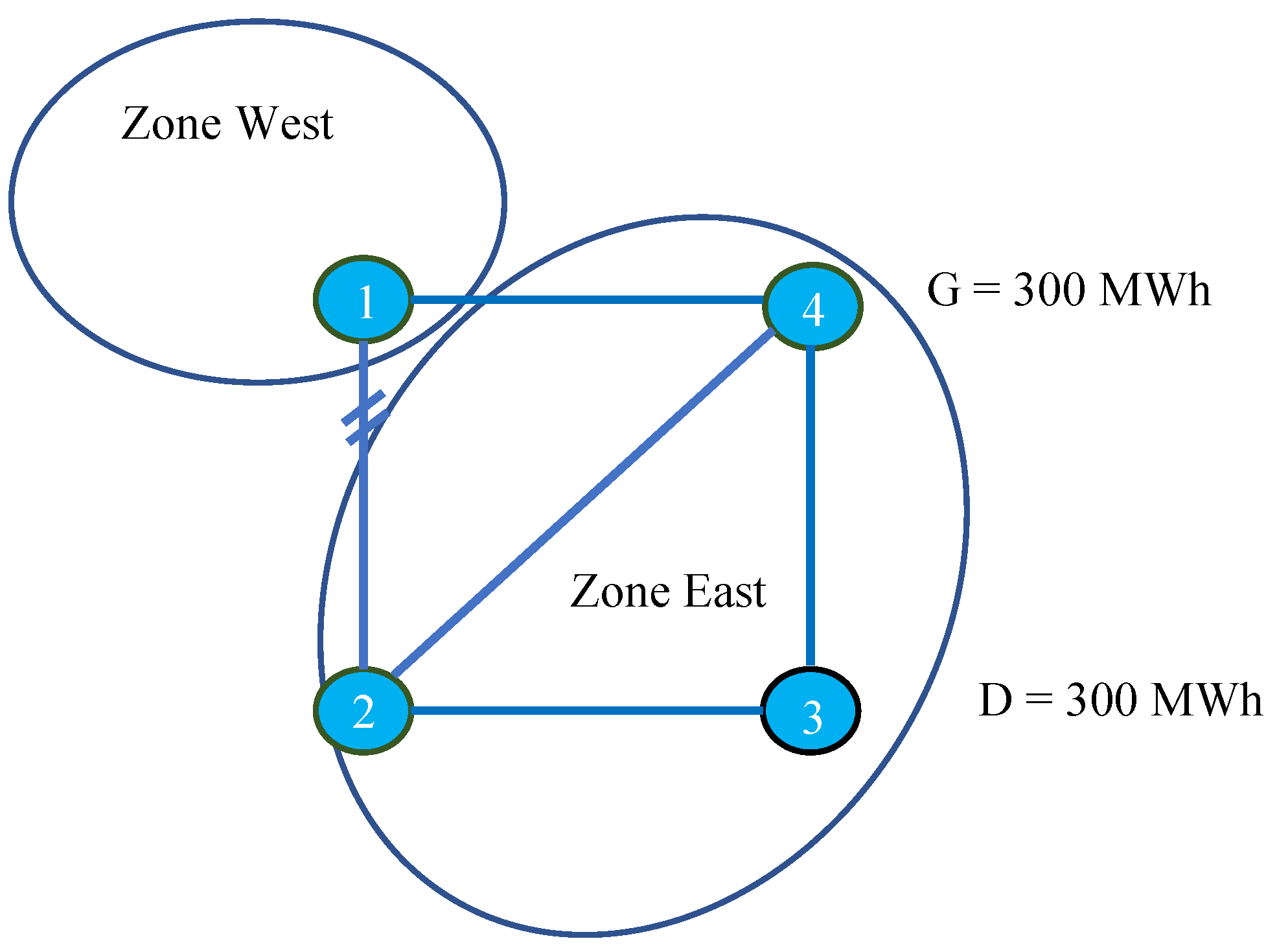
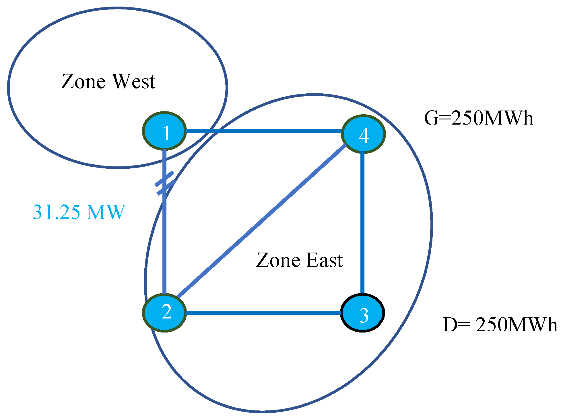
5.3. Joint Auction under Zonal Pricing

5.3.1. Long-Term Market Clearing and Settlements under Zonal Pricing

Using the FRM and GDSK provided in Section 5.2.3 and the base case in Section 5.2.1, Table 6 summarizes the interconnection capacity limits and zonal PTDF associated with each bid in the zonal market input for the long-term auction. We assume that all energy purchase and sale bids within the hub zone have a zonal PTDF value of 0.
Using the bid information in Table 1 and grid modeling parameters in Table 6, the long-term auction is cleared. The long-term auction outcome is depicted in Figure 14. Bid 1 is accepted with 217.8 MWh of FTR; bid 3 is awarded with a 300 MWh energy sale contract; and bid 5 is awarded with a 300 MWh energy purchase contract. Similar to joint auctioning under nodal pricing, the dual variable of the energy balance equation gives the zonal price in the demand zone east: €25/MWh. The shadow price of interzonal transmission link 1–2 is the dual variable of the power flow constraint, which stands at €17.78/MW. The price of FTR for bid 1 is €10/MW (17.78 × 0.5625). The zonal price for zone west is calculated as €15/MWh (25–17.4× 0.575). With the interzonal PTDF set at 0.5625 from zone west to zone east, the estimated flow resulting from cross-zonal trade on interconnection line 1–2 is 122.5 MW. The FRM estimates that flows from cross-zonal and intrazonal trade add up to 200 MW on interconnection 1–2, which reaches its capacity limit.
The payments from bid winners to the SO are summarized in Table 7. Bidder 1 pays €2178 to the SO, while bidder 5 pays €7500 to the SO. Simultaneously, bidder 3 receives €7500 from the SO for its energy sale.

5.3.2. Day-Ahead Market Clearing and Settlements under Zonal Pricing

Contrary to nodal pricing, the dispatch from day-ahead market clearing under zonal pricing is physical, as discussed in Section 3. Consequently, only energy bids and bilateral contracts are permitted in the day-ahead market. Bid 1 is treated as a generation bid from zone west in the day-ahead market with a minimal supply of 217.8 MWh. Similarly, we assume that bidder 1 that has secured 217.8 MWh of FTR in the long-term auction will match it with a bilateral contract between zone west and zone east. Therefore, the energy supply bid from zone west has a lower bound of 217.8 MWh and a higher bound of 500 MWh. As the demand bid is binding in the day-ahead market, both the lower and upper limits of the energy purchase bid from node 3 are set at 500 MWh. The base case and reference flow for the day-ahead market are presented in Section 5.2.2. The zonal PTDF and RAM values resulting from the GDSK and FRM computations in Section 5.2.3 are presented in Table 8. It is crucial to note that the interzonal PTDF value on the congested interconnection 1–2 in the day-ahead auction is lower than that in the long-term auction, as discussed in Section 4.3. The interzonal PTDF on the interconnection elements 1–4 is calculated as (1 − P T D F 1 2   ). Due to the way the PTDF value is calculated in the table, this interconnection line that has unlimited capacity in the case study does not follow the rule of more relaxed PTDF values in the subsequent auctions. Revenue inadequacy may arise in the day-ahead market if this interconnection line also has limited capacity, which is beyond the scope of this paper.
Using the RAM and zonal PTDF values in Table 8 and the revised energy bids discussed in the previous paragraph, the day-ahead market is cleared under the FBMC mechanism. The generation in zone west from day-ahead market clearing is 288.6 MWh, while that in zone east is 211.4 MWh. Zone east has a price of €20/MWh, and the zone west price is €15/MWh. Similar to the long-term auction, the 200 MW on interconnection line 1–2 is the estimated flow based on assumptions such as interzonal PTDF values, reference flow, and FRM at the time of day-ahead market clearing. Line 1–2 has a congestion price of €9.09/MW. The market clearing for the day-ahead timeframe is illustrated in Figure 15.
Following the day-ahead market clearing outcome, the day-ahead generation and load payments to the SO are outlined in Table 9. There is a surplus of €1443 (10,000–4329–4228) for the SO.
After the day-ahead market, the SO should pay the long-term bid winners according to the day-ahead market prices. Payments from the SO to previous auction winners in the day-ahead market are presented in Table 10. The SO pays €1089 to bidder 1, who holds 217.8 MWh FTR from the long-term auction, and €6000 to bidder 5, who holds 300 MWh energy purchase rights. Meanwhile, bidder 3 pays back €6000 to the SO for the 300 MWh of energy sale rights. The SO’s total net payment for the previous auction winners in the day-ahead time frame is €1089. This surplus of €1443 can cover the net payment of €1089 to previous bid winners. Therefore, revenue adequacy for the SO between these timeframes is guaranteed (Revenue adequacy under zonal pricing is defined as the SO’s capability for cost recovery via market-based mechanisms. Section 6 provided more detailed explanations.).

5.3.3. Redispatch Outcomes

Following the day-ahead market clearing, the estimated flow on line 4–3 is 276.4 MW, which exceeds the 250 MW capacity limit, necessitating a redispatch by the TSO. In a national-based redispatch where TSOs can only dispatch resources within their bidding zone, an equal redispatch volume is required at nodes 4 and 2. The generator at node 4 (with downward arrow) is asked to reduce its generation from 211.4 MWh to 105.8 MWh, while the generator at node 2 (with upward arrow) is required to produce 105.6 MWh. The national-based redispatch results are depicted in Figure 16.
The generator at node 4, which is asked to reduce its generation, pays the TSO €2112 for avoided generation costs. This generator also receives €2112, equating to forgone revenue from the day-ahead market. The generator at node 2 is requested to produce 105.6 MWh and is paid €8448. Table 11 summarizes the payments from the TSO to generators in national-based redispatch. The TSO incurs an additional cost of €8448.
During cross-border redispatch, the TSOs require the generator at node 1 to increase generation by 111.4 MWh, that at node 2 to start and dispatch up with 50 MWh, and that at node 4 to dispatch down with 161.4 MWh. The results are presented in Figure 17. Noteworthy, cross-border redispatch exhibits the same dispatch pattern as nodal pricing in the real-time market.
Under cross-border redispatch, the costs for generator 1 dispatching up are €1671, and the costs paid for generator 2 dispatching up are €4000. An avoided cost of €3228 occurs for the generator at node 4, which it needs to pay back to the SO. At the same time, the lost revenue compensation paid to the generator at node 4 from the SO for dispatching down is €3228. Table 12 summarizes the payments from TSOs to generators in cross-border redispatch. The total cross-border redispatch costs are €5671.

6. JETRA Performance Indices and Case Study Evaluation

As long-term market timeframes and hedging instruments are introduced in this research, the following important question arises: How can we assess market outcomes in the multi-timeframe and multi-product auctions to compare performance under zonal and nodal pricing? In Section 6.1, we introduce a comprehensive set of indices to evaluate auction performance, focusing on hedging effectiveness for market players, system operation efficiency, and revenue adequacy for SO in cross-border cooperation. Next, Section 6.2 evaluates the case study for JETRA implementation with the proposed indices. Section 6.3 summarizes the joint auction outcome differences under nodal and zonal pricing from the perspectives of market players and SO.

6.1. JETRA Performance Indices

To compare auction outcomes under nodal and zonal pricing, a comprehensive set of indices is proposed. It should be noted that this case study is not intended as an exhaustive scenario study and does not aim to account for the effects of bidding strategies; rather, it is primarily intended to illuminate and emphasize the causes of different performance when implementing JETRA in different systems.
Conventional market modeling has a well-defined evaluation approach, such as assessing the system operation costs for the timeframe under consideration. JETRA, as multi-timeframe auctions involving hedging and spot market transactions, requires a holistic evaluation approach to assess its performance across various timeframes for different stakeholders.
An important question when introducing a hedging mechanism in the long-term market is how effectively the hedging instruments function; therefore, we are interested in the cumulative costs across different market timeframes incurred by market players under nodal and zonal pricing. In contrast to market studies that focused on one timeframe, this research introduced multi-timeframe market clearing under the condition that market clearings from previous auctions are liquidated. In addition, the auctioning objective is set to maximize bid values. Section 5.1 and Section 5.3 show that the sum of cleared generation and FTR in the same market auction round are not identical under zonal pricing and nodal pricing. Consequently, the total system cost evaluation approach often employed in a single market timeframe is not applicable here. Furthermore, we also explore the causes of different cumulative costs using indices such as the GDSK metric and cross-border trade potential.
The GDSK metric, which implicitly includes the predicted dispatch pattern for a part of the market condition as a deviation from the base case, serves as input for grid modeling and has an impact on the zonal market clearing outcome. Comparing the ex-ante applied GDSK metric with the optimal value helps to measure the accuracy of the predicted grid modeling input and explain sources of system inefficiencies in the dispatch patterns. Cross-border trade potential indicates the amount of lower-cost cross-border energy supply that market players can procure in the forward market or in the last round of JETRA with physical dispatch. In a large geographic area with different renewable resource endowments, the cross-border trade potential enabled by market mechanisms determines how resource complementarity across borders can be best used for an optimized system.
A focal point of this paper is to demonstrate the application of the multi-settlement rule and the importance of consistent market design across timeframes. Following the PTDF and flow limit rules discussed in Section 2, revenue adequacy for SO under nodal pricing can be achieved, which allows cost allocation based on price signals from market mechanisms.
Revenue adequacy for SO under zonal pricing assesses whether cost distribution across borders can be solely based on price signals from the JETRA wholesale market. Furthermore, the revenue gap for SO indicates the amount required to be allocated across borders with pre-negotiated rules outside market mechanisms. This has important implications for the effectiveness of cross-border cooperation under the decentralized market model, when the redispatch costs rise sharply and constitute an important part of the total costs. First, consumers, as the final payer of the total costs, may prefer the coupled wholesale market to function efficiently without an expensive ex-post fix to correct market flaws. Second, while redispatch cost allocation spans across borders, redispatch cost reimbursement is currently subject to national regulations. Those who become welfare-losing countries from the redispatch cost allocation may face difficulties in justifying the payment of those costs incurred abroad with their national regulatory authorities, which may impact their willingness to engage in cross-border trade.
  • The total net payment for demand over various timeframes is calculated to compare the dynamic economic efficiency of using congestion hedging instruments in nodal and zonal pricing markets. In this case study, we assume that the costs of FTR and energy purchases across different timeframes are ultimately borne by the user, who represents the demand at the primary load node.
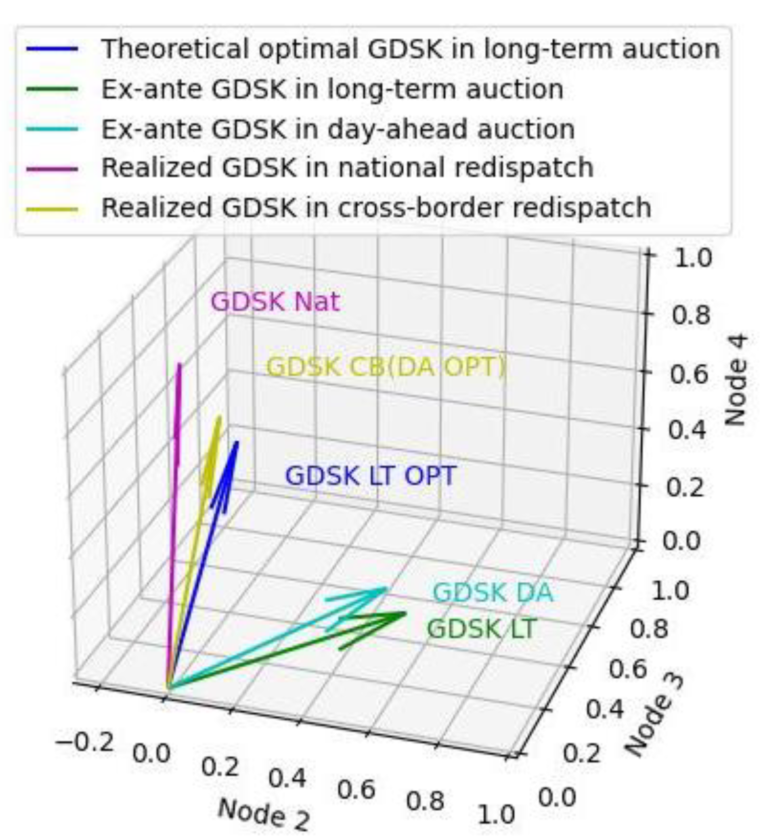
  • The GDSK metric, used as input for each round of zonal market clearing, is compared with the theoretically optimal GDSK calculated ex-post. The GDSK used for grid modeling in the auction presents predicted nodal net changes per unit of zonal net position change. Retrospectively, given the auction clearing outcome under nodal pricing, nodal dispatch is compared with the base case generation load pattern to derive the theoretically optimal GDSK. The realized GDSK metric calculates the realized net export at each node after market clearing and compares it with the base case to compute the GDSK ex-post market clearing. The formula for different GDSK metrics is presented in Appendix D.1. The GDSK metric reveals an important source of inefficiencies in system dispatch under FBMC.
  • Cross-border trade potential: In the forward market, this index evaluates the cross-border trade volume and the potential for market players to use the market to procure hedging instruments across borders. In the market timeframe that has physical dispatch, this index indicates the physical cross-border trade volume enabled by the market design.
  • Revenue adequacy for SO: In the literature, revenue adequacy is defined as the SO’s ability to compensate energy and transmission rights holders from the surplus accrued through energy and transmission rights auctions or generation and load payments. This research extends this concept to include the SO’s capability for cost recovery via market-based mechanisms. Revenue adequacy in JETRA in the day-ahead market under nodal pricing assesses whether energy and transmission right revenue from the day-ahead auction is sufficient for paying the rights holders from the long-term auction. For JETRA in the real-time market under nodal pricing or the day-ahead market under zonal pricing, revenue adequacy assesses whether generation and load net payments suffice to pay the right holders from the previous auction. In the redispatch under zonal pricing, this index measures whether the surplus from the day-ahead market, namely the amount left with the SO after the energy and transmission rights are paid, is enough to pay the redispatch costs.

6.2. Case Study Evaluation

6.2.1. Total Costs

As indicated in Table 13, demand user costs are minimized under nodal pricing. The zonal pricing approach, specifically under the national-based redispatch approach, incurs the highest costs, whereas the cross-border redispatch approach results in intermediate costs. This indicates that hedging functions more effectively for the demand that participates in the JETRA under nodal pricing than under zonal pricing. We further explore the GDSK and cross-border trade indices to explain the total cost differences.
As the cost equation in Appendix D.2 indicates, the total costs for the demand user at node 3 can be decomposed into several parts. Equation (A24) demonstrates the contribution of hedging products, spot market price, and redispatch costs to the total costs. The amount of energy covered by the long-term FTR bid will be charged the day-ahead market price in zone west, and its congestion price is set by the long-term FTR bid price, i.e., the price difference between zone east and zone west in the long-term auction. The amount of energy covered by the long-term energy bid is charged at the long-term wholesale energy price in zone east. The incremental demand increase or decrease in the day-ahead market compared with the long-term bids is charged with the day-ahead market price in zone east. Redispatch costs are not associated with the long-term or day-ahead market price and are added to the total costs after the market closure.

6.2.2. GDSK in the Long-Term, Day-Ahead Markets, and Redispatch Phase

Market clearing results are contingent on the GDSK and zonal PTDF values. In Section 4.2, ex-ante GDSK rules were proposed for maintaining FTR feasibility in grid modeling. The Euclidean distance between the ex-ante GDSKs and the theoretically optimal value indicates economic inefficiency due to information asymmetry by calculating the disparity between the two. As the equations in Appendix D.1 indicate, the realized GDSK metric calculates the realized net export at each node after market clearing and compares it with the base case to compute the GDSK. As already mentioned in Section 2, the realized GDSK often deviates from the ex-ante applied GDSK, which makes the ex-ante identification of intrazonal critical network elements difficult. Table 14 presents the ex-ante applied GDSK, realized GDSK, theoretically optimal GDSK values, and Euclidean distance between the applied and optimal values for the long-term and day-ahead markets.
During the long-term auction, a more conservative GDSK is used due to heightened uncertainty. Consequently, the set of generation and load anticipated to respond to net zonal exchange under zonal pricing differs from the optimal under nodal pricing. The Euclidean distance is 0.729 between the ex-ante GDSK and the optimal value in the long-term auction. In the day-ahead market, the optimal GDSK exhibits a different pattern compared to both the ex-ante value and the optimal GDSK in the long-term. We anticipate node 2 to be a main energy withdrawal node with net zonal import in zone west. However, under nodal pricing, generator at node 2 starts to generate at the day-ahead load level to alleviate congestion. This demonstrates the non-linear characteristics of the optimal GDSK to accommodate grid congestion and complexity of approximating it with ex-ante applied values. The Euclidean distance is 0.725 between ex-ante and the optimal GDSKs in the day-ahead market.
The redispatch phase, implemented after the spot market closure, can be considered a mechanism employed by TSOs to amend the ex-ante determined GDSK metric. Adopting a nodal grid view, this process alleviates congestion, effectively forming another set of realized GDSKs that deviate from the values used in the day-ahead auction. This ex-post adaptation of GDSK by TSOs suggests not only a change in the dispatch pattern from the wholesale market but also an incursion of redispatch costs.
Following the day-ahead market clearing, the estimated flow on line 4–3 amounts to 276.4 MW, which necessitates a redispatch by the TSO in this case study. The ex-post GDSK at the redispatch stage is derived by comparing the national-based or integrated redispatch outcome, as illustrated in Figure 16 and Figure 17, with the base case used in the day-ahead market demonstrated in Figure 13 (During the national-based redispatch, the generator at node 2 exhibits increases in production corresponding to the rise in imports in the zone east of the base case. This leads to a negative sign at node 2 in the GDSK metric). Table 15 presents the GDSK across the two redispatch approaches and compares the values with the optimal GDSK for the day-ahead market under nodal pricing.
  • The Euclidean distance between the ex-post GDSK derived from the national redispatch and the theoretically optimal GDSK for the day-ahead auction is 0.34. The ex-post GDSK value obtained through national redispatch also allows for consideration of grid congestion in generation load patterns. This reduces the Euclidean distance of the ex-ante GDSK metric from the theoretically optimal value, which is 0.725 in the day-ahead market.
  • The cross-border redispatch in Figure 17 aligns with the real-time nodal pricing market outcome in Figure 9 in Section 5.1.2, signifying that the realized GDSK following the cross-border redispatch matches the theoretically optimal GDSK.
  • When we view the GDSK distance together with total costs, the closer the realized redispatch GDSK is to the optimal value, the lower the total costs for the demand at node 3.
As shown in Figure 18, the ex-ante computed GDSK values for grid modeling in long-term auctions, day-ahead markets under zonal pricing, and the realized GDSK in the national redispatch display a notable divergence from the theoretically optimal values derived from nodal pricing dispatch.

6.2.3. Cross-Border Trade in Long-Term and Day-Ahead Markets

In this case study, long-term cross-border trade is conducted through bilateral contracts with FTR bidding. Table 16 lists the cross-border FTRs cleared in the long-term and day-ahead auctions under both nodal and zonal pricing. The potential optimal interzonal transaction, derived using the applied RAM and the theoretical optimal zonal PTDF calculated from the theoretical optimal GDSK, is presented in the third column. The fourth column displays the interconnection utilization rate for interconnections 1–2 under zonal pricing, which accounts for the combined utilization from both cross-border and intrazonal trade in the market clearing.
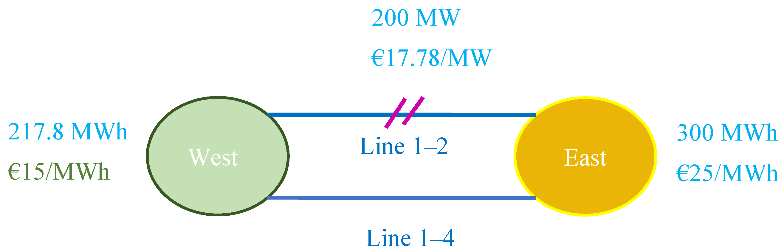
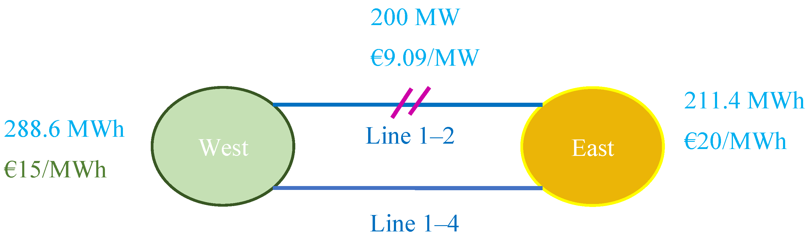
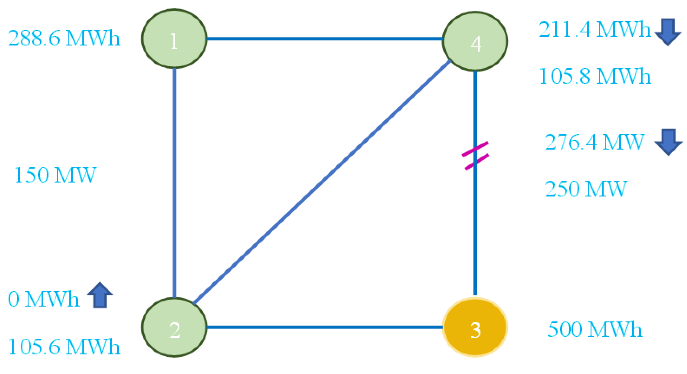
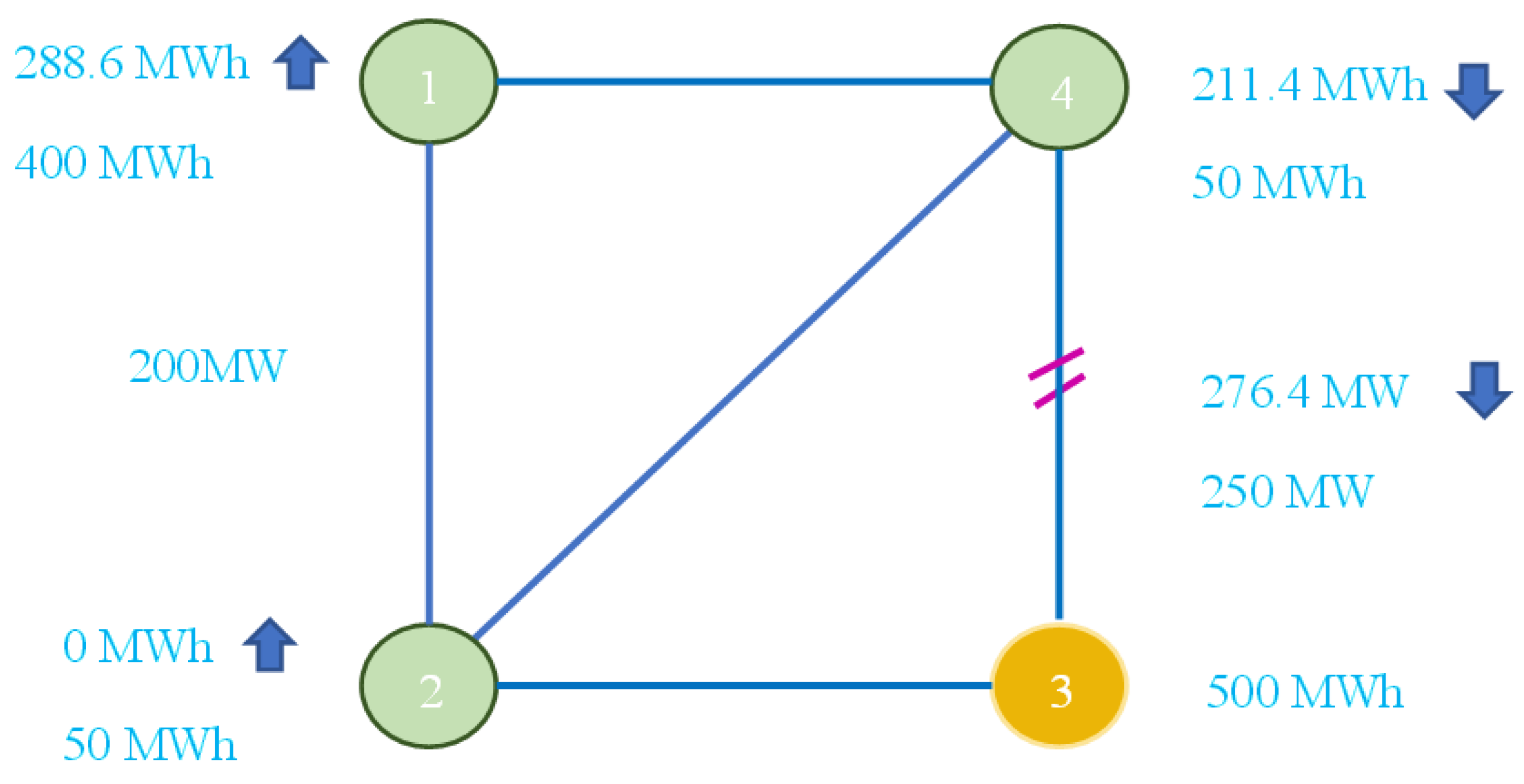
  • The cross-border zonal trade with an accepted FTR bid of 217.8 MWh in the long-term auction falls significantly short of the 375 MWh FTR obtained under nodal pricing. This discrepancy arises because of two factors, namely: the larger volume of FRM applied and a more restrictive GDSK rule in the long-term auction, which factors in higher uncertainties in the timeframe. During the day-ahead timeframe, the cleared cross-border trade amounts to 288.6 MWh. This improvement is facilitated by the more relaxed GDSK rules and the reduced FRM value applied in the RAM calculation.
  • The divergence between the cleared cross-border trade and the potential optimal interzonal transaction indicates the improvement of cross-border trade when the theoretical optimal GDSK is applied. The difference between potential optimal interzonal transactions and cross-border trade under nodal pricing demonstrates the influence of RAM calculation on the potential for cross-border trade.
  • Figure 8 and Figure 9 illustrate that the interconnection line 1–2 is fully utilized under nodal pricing. However, under zonal pricing, this interconnection has a lower utilization rate due to conservative grid modeling.

6.2.4. Revenue Adequacy

The conservative grid model developed in accordance with the rules described in Section 4.2, eliminates the need for redispatch to alleviate interconnection congestion that arises from cross-border trade. Nevertheless, redispatch costs are incurred because of intrazonal network constraints (i.e., the congested network element 4–3 in the case study). The SO balance after the day-ahead market accounts for the surplus from load payments and generation costs after payments are made to the long-term bid winners. Table 17 details the SO balances following the day-ahead market and the ensuing redispatch costs.
Irrespective of whether a national-based or cross-border redispatch is implemented, redispatch costs invariably exceed the SO balance after the day-ahead market. Therefore, the SO’s revenue adequacy cannot be sustained post-redispatch. As a result, allocating redispatch costs across different jurisdictional areas using administratively negotiated rules becomes necessary.
While cross-border redispatch can reduce the total system costs under zonal pricing compared with national redispatch, it requires a centralized operation that uses a nodal grid to dispatch the resources in the whole system as an ex-post fix to the wholesale market flaw. Even if a centralized redispatch operation can be executed through strengthened cross-border cooperation by TSOs, which adds to the total costs for market participants, it raises the question of why the centralized market model is not implemented in the wholesale market.
Under nodal pricing (as detailed in Section 5.1), revenue from energy and transmission rights sold in the day-ahead auction matches the payments made to holders of long-term auction rights. Similarly, net payments from generation and load in the real-time market balance the payments made to right holders from the day-ahead auction.
In summary, with respect to nodal pricing, revenue adequacy is maintained in both day-ahead and real-time markets for ISO. By contrast, under zonal pricing, while revenue adequacy is preserved for the SO in the day-ahead market, it cannot be maintained following redispatch.

6.3. Observations Regarding Zonal Market Outcomes

The case study reveals the comparatively less efficient performance of JETRA under zonal pricing as opposed to nodal pricing. Some observations regarding zonal market outcomes are as follows:
  • From the SO’s standpoint, there is less interconnection capacity used for cross-border trade under zonal pricing than under nodal pricing. In addition, the case study reveals that intrazonal trade patterns and intrazonal networks that are not well represented in the zonal grid model necessitate redispatch. The redispatch costs challenge revenue adequacy, and the cost gap must be allocated across borders according to administratively negotiated rules.
  • From the grid user’s perspective, the hedging function of long-term cross-border transmission rights and energy contracts is significantly weaker under zonal pricing compared with that under nodal pricing. The diminished potential for cross-border trade under zonal pricing is a crucial factor behind this difference. Another contributing factor is the varying levels of granularity of the network constraints used in the optimization process. Under the zonal model, the nodal grid view is solely implemented in the redispatch, where buyer bids are no longer accessible to market participants. Thus, transmission rights and energy contracts issued from joint auctioning, based on the zonal model in long-term auctions, cannot hedge against redispatch costs incurred post-market closure. This predicament raises the question of whether implementing auction energy contracts and transmission rights to link long-term and day-ahead markets alone can create effective hedging instruments under zonal pricing. For the hedging instruments to work more effectively, consistent grid modeling and market rules are required.
A weaker performance of JETRA under zonal pricing can be observed as opposed to nodal pricing for both SO and market players. An in-depth analysis of the case study in this section reveals that the inefficiencies of JETRA implementation under zonal pricing are related to the institutional settings and how zonal pricing market clearing is designed, which is exacerbated in the long-term auction when a hedging mechanism is introduced. To address these issues, a holistic market reform is required.

7. Conclusions and Policy Implications

In Europe, the societal and policy drive for decarbonization calls for a higher share of renewable energy integration with well-developed cross-border markets. Simultaneously, electricity market development in Europe has transitioned from a focus on short-term competition to long-term hedging.
For long-term, cross-border market development, this research advocates the co-development of cross-border PPAs and forward market coupling. We propose the JETRA model developed by O’Neill et al. as the pivotal mechanism for the long-term, cross-border market in Europe because it supports the two contract forms in the long-term auction and gives market players the flexibility to choose. However, the success of developing an effective long-term market through JETRA depends on the underlying market structure.
Is the zonal pricing-based FBMC currently implemented in the European cross-border market conducive to establishing the proposed long-term market? The link between the long-term and short-term markets has never been so important, yet the challenges facing these markets differ. Our research investigated two critical challenges associated with implementing JETRA under FBMC:
  • Increased uncertainties in JETRA grid modeling: The inherent methodological dilemma of FBMC lies in the information asymmetry between the TSO and market players for grid modeling. Our analysis of the challenges in computing key grid modeling parameters—base case and zonal PTDF—reveals that this information asymmetry becomes particularly critical for JETRA grid modeling in long-term auctions. Simultaneously, the obligation to ensure the firmness of cross-border FTRs auctioned in JETRA, acting as a prerequisite for safeguarding long-term contract integrity, poses substantial challenges for TSOs. The combined effect of these is conservative grid modeling, inefficient dispatch, and low interconnection utilization, as demonstrated by the case study.
  • Limited applicability of multi-settlement rules: In the zonal pricing setting of the case study, which adheres to the current European market design, physical dispatch starting from the day-ahead market dictates that the multi-settlement rule can only link the forward markets with the day-ahead market. Furthermore, market participants who hold long-term hedging products cleared with a zonal grid model cannot effectively hedge against redispatch costs incurred using a nodal grid model, weakening the overall effectiveness of hedging strategies. The high redispatch costs also render the granular cost allocation across borders based on market price signals, a key advantage of multi-settlement rules under nodal pricing, impracticable in the current zonal pricing framework.
Is the current institutional setting fit for the purpose of establishing a long-term, cross-border market? The current market coupling mechanism, designed around zonal pricing in the day-ahead market, determines institutional functions and exerts a profound impact on the organization of the long-term market. We have highlighted how the current institutional functions for market clearing create information asymmetry, exacerbating inefficiencies in grid modeling when JETRA is implemented in the long-term market. The long-term, cross-border market that introduces significant challenges, thereby acts as a game-changer for the European decentralized market model.
The policy implications derived from the analysis of the market structure required for JETRA implementation are multifaceted. Our research emphasizes the need to transition from zonal pricing to nodal pricing in the European electricity market to establish an efficient, long-term market. This shift would require the simultaneous optimization of network and market conditions. Furthermore, the effective implementation of multi-settlement rules necessitates the use of consistent grid models and the resetting of the relationship between market outcomes across different timeframes.
In this research, we have not discussed the design aspects of auctions. For instance, the bids associated with energy supply, or FTR, are backed by physical generation assets in the case study. The potential role of financial bids in JETRA should be investigated. The stochastic nature of network capacities in the long-term auction is not considered in this research. This should also be examined for JETRA implementation.

Author Contributions

D.H.: conceptualization, methodology, and writing; G.D.: supervision and reviewing. All authors have read and agreed to the published version of the manuscript.

Funding

This research received no external funding.

Data Availability Statement

Data are contained within the article.

Acknowledgments

The authors are grateful to Luis Olmos and Erik Delarue for their discussions and feedback.

Conflicts of Interest

The authors declare no conflicts of interest.

Appendix A

Appendix A presents the mathematical formulation for JETRA. The JETRA model maximizes the value of accepted bids, including flow gate rights, point-to-point financial transmission rights, and energy sale/purchase contracts. Constraints in auction optimization include load flow limitations and an equilibrium between energy supply and demand. Bidders are required to provide offer prices along with lower and upper boundaries for bidding quantities of energy sales and purchases as well as transmission rights. In this study, DC load flow constraints are used. The network typology remains consistent across different timeframes. The mathematical formulation of the auction model is summarized by the following formula:
M a x   b 1 t 1 + b 2 t 2 + b 3 t 3 + b g g
β 1 t 1 + β 2 t 2 + β 3 t 3 + β g g F               ( μ )
α 2 t 2 + τ g = 0                 ( λ )
T L P t p T U P , p = 1 , 2 , 3 ; G L p g G U p
where:
t 1 is a vector of the flow gate rights awarded to bidders; and t 1 i represents the ith bid by bidders to obtain rights and collect revenues from one or a portfolio of transmission element constraints. The terms flow gate rights and PTRs are interchangeably used in this research to refer to the rights for physical capacity on certain transmission elements. Bidders can specify the highest and lowest amount with T 1 L j and T 1 U j , respectively.
t 2 represents a vector of the point-to-point financial transmission right obligation awarded to bidders; and t 2 j represents the jth bid for the right to collect or pay for nodal price differences between the designated node pairs in the designated period. Bidders can specify the lowest and highest amount of transmission rights they want to obtain with T 2 L j and T 2 U j , respectively. The net injection for bid is defined as α 2 j t 2 j and α 2 is defined as the row vector α 2 j .
t 3 is a vector of point-to-point financial transmission options; and t 3 k represents the kth bid for the option to collect the nodal price difference between specified nodes. Bidders can specify the lowest and highest amount of transmission rights that they want to obtain with T 3 L K and T 3 U K , respectively.
g is a vector of energy sale or purchase bids awarded to bidders. The lower and upper values of the bidder are given in the bid and represented by G L and G U , respectively.
β 1 , β 2 ,  β 3 , β g is a vector of the transmission rights required on each transmission element per unit of each bid type. It is also called the PTDF per unit of transaction. β 1 i h t 1 i is the transmission capacity required on the transmission element h per unit value of the ith bid for flow gate rights. β 2 j h t 2 j is the transmission flow induced per unit of financial transmission right bid t 2 j on the transmission element h. β 3 j h t 3 j is the transmission flow induced per unit of financial transmission option bid t 3 j on the transmission element h. Below, we discuss why we do not use the financial transmission option in this research. β g g represents the flow created on the transmission element by energy purchase and sale bids.
F is a vector of the capacity limits of the transmission network.
μ is a vector of the dual variables of the transmission constraints. For each transmission constraint, there is a dual representing the shadow price for transmission congestion.
τ is a vector of ones.
λ is the marginal cost of meeting demand at the hub node defined for the PTDF calculation.
To maintain revenue adequacy, point-to-point FTR options t 3 is limited to the sum of FGRs with only positive PTDF values across the transmission components. However, as the analysis of O’Neill et al. demonstrates, such point-to-point financial transmission options are likely to result in a lack of interest from market participants compared with FGR, especially under the conservative assumption of positive PTDFs. A market participant who must choose between an FTR option and an FGR pays the same amount for both but receives less in return from the FTR option [1]. Therefore, this type of right is omitted from the case study.

Appendix B. Base Case and Zonal PTDF Impact on Outcome

Appendix B demonstrates the impact of the selected base case and zonal PTDF on the interconnection and intrazonal network flow estimation in the zonal market model, as opposed to the real flow incurred because of the market clearing outcome. These case studies are inspired by the research from Felten et al., which investigates the impact of grid parameter input on the feasible line region [24].

Appendix B.1. Case A: Nodal Dispatch Intrazonal Trade Pattern as a Base Case

This case illustrates that with an ideal base case and perfect PTDF derived from nodal market clearing from Section 5.1, the design of the zonal market clearing algorithm may not guarantee the desired firmness of cross-border FTR. Therefore, the use of FRM to account for uncertainties in the calculation process is necessary with a joint auction model under zonal pricing.
The base case in this scenario adopts the ideal intrazonal trade pattern depicted in Figure A1, derived from nodal market clearing during the long-term auction in Figure 8.
Figure A1. Perfect base case with intrazonal trade equivalent to nodal market clearing.
Energies 17 01923 g0a1
The SO is assumed to have perfect insights, which enable it to understand that energy demand is solely located at node 3 and that the net zonal export from west to east results in demand increasing at node 3. With the GDSK set at (0, 1, 0) between nodes 2, 3, and 4 and a zonal PTDF of 0.5, the intrazonal trade generates a flow of 12.5 MW on line 1–2. The RAM, without setting the FRM, is 187.5 MW.
The flow constraint computed to determine the interzonal trade domain while considering the base case pattern is represented by the following equations:
212.5 0.5 × E x 187.5
  425 E x 375
The volume of interzonal transactions cleared through the zonal market is 375 MWh, whereas the cleared intrazonal trade within zone east amounts to 300 MWh. This discrepancy occurs between the cleared intrazonal trade and the base case because the zonal PTDF of intrazonal trade is set at 0.
The resulting flow on interconnections 1–2 is 225 MW, which exceeds the interconnection limit of 200 MW. Consequently, redispatch or curtailment of cross-border FTR is required to alleviate interzonal line congestion. Meanwhile, the flow on intrazonal line 4–3 is 375 MW, surpassing the line limit of 250 MW.

Appendix B.2. Case B: Overly Relaxed GDSK Assumption and Small Zonal PTDF

The base case in Figure A2 perfectly matches the intrazonal trade in the long-term auction under zonal pricing depicted in Figure 14. The GDSK assumption made in the case study is more relaxed compared with the realized GDSK (0, 1, 0) among node 2, node 3 and node 4 in the long-term auction. Having an overly relaxed GDSK metric in the import zone results in a smaller zonal PTDF in the grid modeling, which leads to an underestimation of interconnection flow in the market model and an overly optimistic feasible region for interzonal trade. The resulting interconnection congestion because of the cleared dispatch may lead to curtailment of the allocated cross-border FTR. Thus, one seeks to avoid an overly relaxed GDSK metric in JETRA grid modeling.
Figure A2. Base case for case B and case C.
Energies 17 01923 g0a2
As illustrated in Figure A2, the base case for both Cases B and C includes an intrazonal trade of 300 MW from node 4 to node 3. Assume that the GDSK between nodes 2, 3, and 4 is (0, 0.5, 0.5), with a zonal PTDF of 0.4375. This GDSK selection implies that a unit zonal export from west to east is offset by a 0.5 MW decrease in generation at node 4 and an increase in 0.5 MW demand at node 4.
The flow constraints for determining the interzonal trade domain, while considering the base case pattern, are expressed as follows:
237.5   0.4375 × e x 162.5
542.8 e x 371.43
The volume of interzonal transactions cleared through zonal market clearing reaches 371.43 MWh, whereas the cleared intrazonal trade within zone east reaches 300 MWh. The unachievable GDSK in zone east leads to overly lenient assumptions for the zonal PTDF, which underestimates the effects of interzonal trade on the interconnection capacity. The decrease in generation at node 4, in relation to variations in net zonal exchange and possessing the lowest nodal PTDF value on line 1–2, is overestimated during the GDSK computation. Consequently, the estimated zonal PTDF value of 0.4375 is lower than the actual value of 0.5.
The resulting flow on interconnections 1–2 is 223.2 MW, which exceeds the interconnection limit of 200 MW. Meanwhile, the flow on intrazonal line 4–3 reaches 373.2 MW, which exceeds the line limit of 250 MW. Because the adopted base case perfectly aligns with intrazonal trade resulting from market clearing, the intrazonal flow can be perfectly estimated in the process of computing the feasible region, as demonstrated in A7. This can be interpreted as exceeding interzonal trade cleared in the market model, which leads to intrazonal congestion. Consequently, the redispatch or curtailment of cross-border FTR becomes necessary for alleviating interzonal and intrazonal congestion.

Appendix B.3. Case C: Overly Stringent GDSK Assumption and Large Zonal PTDF

This case study also uses the base case shown in Figure A2. In contrast to case B, it demonstrates the effect of stringent GDSK input on interzonal flow estimation and interconnection capacity utilization.
Assuming that all exports from zone west to zone east are counterbalanced by an increase in demand or a decrease in generation at node 2, the GDSK in zone east stands at (1, 0, 0), and the zonal PTDF is 0.625.
The following flow constraint is used to determine the interzonal trade domain:
237.5 0.625 × e x 162.5
380 e x 260
The maximum net export position is 260 MWh. During zonal market clearing, 260 MWh of FTR is allocated from zone west to zone east. Bid 3, offering a 300 MWh energy sale, and bid 5, proposing a 300 MW energy purchase, are accepted within zone east. Due to the stringent GDSK, the dispatch clearing result is 167.5 MW of interconnection flow on line 1–2, leading to the underutilization of the interconnection line. This zonal dispatch results in a flow of 317.5 MW on intrazonal line 4–3, which exceeds its capacity limit of 250 MW.

Appendix C. Physical Feasibility of Energy and Transmission Rights in JETRA

Appendix C provides proof for the physical feasibility of the previously allocated rights in the later auctions. Suppose that in the earlier round of auction s + 1, the PTR, FTR, and energy bid vectors are denoted by t 1 s + 1 , t 2 s + 1 , and t g s + 1 . The associated PTDF vectors for PTR, FTR, and energy bid vectors are denoted by β 1 s + 1 , β 2 s + 1 , and β g s + 1 . The network flow limit vector is denoted by F s + 1 .
β 1 s + 1 t 1 s + 1 + β 2 s + 1 t 2 s + 1 + β g s + 1 t g s + 1   F s + 1
In the subsequent round of auction s, the PTR, FTR and energy bid vectors are denoted by t 1 s , t 2 s + , and t g s . The associated PTDF vectors for PTR, FTR and energy bid vectors are denoted by β 1 s , β 2 s , and β g s . The network flow limit vector is denoted by F s .
We follow the rules set by the original JETRA design, which requires that the PTDF in the previous round be greater than or equal to the PTDF in the subsequent round. The flow limit on the critical branches in the subsequent round of auction must be greater than or equal to the flow limit in the preceding round. The physical feasibility we provide here is only valid under zonal pricing for critical branches with a limited capacity limit and whose PTDF in the preceding auction round is greater than or equal to that of the subsequent auction.
β 1 s   β 1 s + 1
β 2 s   β 3 s + 1
β g s   β g s + 1
F s + 1   F s
The transmission constraints of the critical branches in the subsequent auction are given by:
β 1 s t 1 s + β 2 s t 2 s + β g s t g s F s
β 1 s t 1 s + 1 + β 2 s t 2 s + 1 + β g s t g s + 1   β 1 s + 1 t 1 s + 1 + β 2 s + 1 t 2 s + 1 + β g s + 1 t g s + 1   F s + 1 F s
The left part of Equation (A17) represents the potential flow resulting from the rights auctioned in the preceding auction, following the PTDF values in the subsequent auction. This value is smaller than or equal to the flow incurred in the preceding auction, which itself is smaller than or equal to the network capacity limits in both the preceding and subsequent auctions.

Appendix D. GDSK Calculation and Total Cost Decomposition for JETRA Indices

Appendix D presents the GDSK calculation and total cost decomposition for demand users in the case study.

Appendix D.1. GDSK Calculation

The theoretical optimal GDSK can be derived from (A18).
T h e o r e t i c a l   o p t i m a l   G D S K = q i n o d a l q i b c q n e t   z o n a l   e x c h a n g e
where
q i n o d a l is the net export at node i under nodal pricing;
q i b c is the base case net export at node i;
q n e t   z o n a l   e x c h a n g e is the net zonal exchange.
The realized GDSK can be written as (A19).
R e a l i z e d   G D S K = q i r e a l i z e d q i b c q n e t   z o n a l   e x c h a n g e
q i r e a l i z e d is the realized net export at node i after zonal market clearing;
q i b c is the base case net export at node i;
q n e t   z o n a l   e x c h a n g e is the net zonal exchange.

Appendix D.2. Total Cost Decomposition

The total payment from the demand user to the SO in the long-term auction can be written as (A20).
T P L = Q L 1 × L M P E L L M P W L + Q L 5 × ( L M P E L )
where
T P L is the total payment from the demand user to the system operator in the long-term auction;
Q L 1 is the accepted volume from bidder 1 that bids for the FTR between zones west and east;
Q L 5 is the accepted bid volume from bidder 5 that bids for energy purchases in zone east:
L M P E L is the locational marginal price from zone east in the long-term auction;
L M P W L is the locational marginal price from zone west in the long-term auction.
The total payment from the demand user to the SO in the day-ahead market can be written as (A21).
T P D = L M P E D × L D = Q L 1 × L M P E D + L D Q L 1 × L M P E D
where
T P D is the total payment from the demand user to the SO in the day-ahead market;
L D is the load level at the day-ahead market;
L M P E D is the locational marginal price in zone east.
The total payback from the SO to the demand user upholding previously allocated rights in the day-ahead market can be written as (A22).
T R D = Q L 1 × L M P E D L M P W D + Q L 5 × L M P E D
where
T R D is the total payment in the day-ahead market from the SO to the long-term bid winners;
L M P W D is the locational marginal price in zone west.
Combining (A21) and (A22), the net payment from the demand user to the SO in the day-ahead market can be written as (A23).
T P D = Q L 1 × L M P W D + ( L D Q L 1 Q L 5 ) × L M P E D
where
T P D is the net payment from the demand user to the SO in the day-ahead market;
The total payment for the demand user across timeframes is the sum of net payments from long-term, day-ahead, and redispatch costs. It can be written as (A24).
T C = Q L 1 × L M P W D + Q L 1 × L M P E L L M P W L + Q L 5 × L M P E L +   L D Q L 1 Q L 5 × L M P E D + R E S P
where
T C is the total cost for the demand user across different timeframes;
R E S P is the redispatch cost.

References

  1. European Commission. Communication from the Commission to the European Parliament, the European Council, the Council, the European Economic and Social Committee and the Committee of the Regions: REPowerEU Plan. EC Website. 2022. Available online: https://commission.europa.eu/strategy-and-policy/priorities-2019-2024/european-green-deal/repowereu-affordable-secure-and-sustainable-energy-europe_en (accessed on 1 February 2024).
  2. Pexapark. European PPA Market Outlook 2023: Navigating the Energy Transition Peaks and Valleys: A Shock-Therapy for Renewables and a Lesson to Remember. Pexapark Website. 2023. Available online: https://pexapark.com/european-ppa-market/ (accessed on 23 March 2023).
  3. European Commission. Proposal for a Regulation of the European Parliament and of the Council amending Regulations (EU) 2019/943 and (EU) 2019/942 as well as Directives (EU) 2018/2001 and (EU) 2019/944 to Improve the Union’s Electricity Market Design. Strasburg. 2023. Available online: https://eur-lex.europa.eu/legal-content/EN/TXT/PDF/?uri=CELEX:52023PC0148 (accessed on 15 March 2023).
  4. European Commission. Commission Regulation (EU) 2016/1719 of 26 September 2016 Establishing a Guideline on Forward Capacity Allocation. Brussels. 2016. Available online: https://eur-lex.europa.eu/legal-content/EN/TXT/PDF/?uri=CELEX:32016R1719 (accessed on 1 February 2024).
  5. Meeus, L.; Schittekatte, T. Who gets the rights to trade across borders? In The Evolution of Electricity Markets in Europe, 1st ed.; Edward Elga: Cheltenham, UK, 2020; pp. 25–42. [Google Scholar] [CrossRef]
  6. ACER. ACER to Consult on the Harmonised Allocation Rules for Long-Term Electricity Transmission Rights. ACER Website. 2023. Available online: https://www.acer.europa.eu/news-and-events/news/acer-consult-harmonised-allocation-rules-long-term-electricity-transmission-rights (accessed on 1 February 2024).
  7. Hogan, W. Restructuring the Electricity Market: Institutions for Network Systems (Working paper, John F. Kennedy School of Government, 02138). Harvard University, Cambridge, MA, USA. 1999. Available online: https://scholar.harvard.edu/whogan/files/hjp0499.pdf (accessed on 1 February 2024).
  8. Jamasb, T.; Nepal, R.; Davi-Arderius, D. Electricity Markets in Transition and Crisis: Balancing Efficiency, Equity, and Security; Working Paper/Department of Economics, Copenhagen Business School No. 04-2023CSEI Working Paper No. 2023; Department of Economics, Copenhagen Business School: Frederiksberg, Denmark, 2023; Available online: https://research-api.cbs.dk/ws/portalfiles/portal/87935064/tooraj_jamasb_et_al_working_paper_04_2023.pdf (accessed on 1 February 2024).
  9. D’Aertrycke, G.; Smeers, Y. Transmission Rights in the European Market Coupling System: An Analysis of Current Proposals. In Financial Transmission Rights: Analysis, Experiences and Prospects (Lecture Notes in Energy, 7); Springer: London, UK, 2013; pp. 333–375. [Google Scholar] [CrossRef]
  10. Spodniak, P.; Collan, M.; Makkonen, M. On Long-Term transmission rights in the Nordic electricity markets. Energies 2017, 10, 295. [Google Scholar] [CrossRef]
  11. Beato, P. Long Term Interconnection, Transmission Rights and Renewable Deployment (RSC Working Paper 2021/57); Florence School of Regulation: Florence, Italy, 2021; Available online: https://hdl.handle.net/1814/71818 (accessed on 1 February 2024).
  12. Van Den Bergh, K.; Boury, J.; Delarue, E. The Flow-Based Market Coupling in Central Western Europe: Concepts and Definitions. Electr. J. 2016, 29, 24–29. [Google Scholar] [CrossRef]
  13. Schönheit, D.; Kenis, M.; Lorenz, L.; Möst, D.; Delarue, E.; Bruninx, K. Toward a Fundamental Understanding of Flow-Based Market Coupling for Cross-Border Electricity Trading. Adv. Appl. Energy 2021, 2, 100027. [Google Scholar] [CrossRef]
  14. Purchala, K. EU Electricity Market: The Good, the Bad and the Ugly. In PSE Website. 2018. Available online: https://www.pse.pl/documents/31287/20965583/PSE_16102018_The_good_the_bad_the_ugly.pdf (accessed on 1 February 2023).
  15. Eicke, A.; Schittekatte, T. Fighting the Wrong Battle? A Critical Assessment of Arguments against Nodal Electricity Prices in the European Debate. Energy Policy 2022, 170, 113220. [Google Scholar] [CrossRef]
  16. O’Neill, R.P.; Helman, U.; Hobbs, B.F.; Stewart, W.R.; Rothkopf, M.H. A Joint Energy and Transmission Rights Auction: Proposal and Properties. IEEE Trans. Power Syst. 2002, 17, 1058–1067. [Google Scholar] [CrossRef]
  17. Huang, D.; Deconinck, G. Coupling European Long-Term Electricity Market with Joint Energy and Transmission Right Auction—Institutional Setting, Market Mechanism and Grid Modelling Comparison between Nodal Pricing and Flow Based Zonal Pricing. In Proceedings of the 7th AIEE Energy Symposium: Current and Future Challenges to Energy Security—The Energy Crisis, the Impact on Transition Roadmap, Virtual Conference, 14–16 December 2022; Italian Association of Energy Economists (AIEE): Rome, Italy, 2022; pp. 136–168. Available online: https://www.aieesymposium.eu/wp-content/uploads/2023/01/BOOK-SYMPOSIUM_2022.pdf (accessed on 1 February 2024).
  18. Smeers, Y.; Study on the General Design of Electricity Market Mechanisms Close to Real Time. Creg Website. 2008. Available online: https://www.creg.be/sites/default/files/assets/Publications/Studies/F810UK.pdf (accessed on 1 February 2024).
  19. Oren, S.S. Point to Point and Flow-Based Financial Transmission Rights: Revenue Adequacy and Performance Incentives. In Financial Transmission Rights Analysis, Experiences and Prospects Lecture Notes in Energy; Springer: London, UK, 2012; pp. 77–94. [Google Scholar] [CrossRef]
  20. Hogan, W.W. Contract Networks for Electric Power Transmission. J. Regul. Econ. 1992, 4, 211–242. [Google Scholar] [CrossRef]
  21. Chao, H.P.; Peck, S.C. A Market Mechanism for Electric Power Transmission. J. Regul. Econ. 1996, 10, 25–59. [Google Scholar] [CrossRef]
  22. O’Neill, R.P.; Helman, U.; Hobbs, B.F.; Rothkopf, M.H.; Stewart, W.R. A Joint Energy and Transmission Rights Auction on a Network with Nonlinear Constraints: Design, Pricing and Revenue Adequacy. In Financial Transmission Rights Analysis, Experiences and Prospects Lecture Notes in Energy; Springer: London, UK, 2012; pp. 95–127. [Google Scholar] [CrossRef]
  23. De Hauteclocque, A. Long-term contracts across Member States: The problem of priority access to interconnectors. In Book Market Building through Antitrust; Edward Elgar: Cheltenham, UK, 2013. [Google Scholar] [CrossRef]
  24. Felten, B.; Osinski, P.; Felling, T.; Weber, C. The Flow-Based Market Coupling Domain—Why We Can’t Get It Right. Util. Policy 2021, 70, 101136. [Google Scholar] [CrossRef]
  25. O’Neill, R.P.; Helman, U.; Hobbs, B.F.; Baldick, R. Independent system operators in the USA: History, lessons learned, and prospects. In International Experience in Restructured Electricity Markets: What Works, What Does Not and Why? Elsevier: Amsterdam, The Netherlands, 2006; pp. 479–528. [Google Scholar]
  26. Glachant, J.; Ruester, S. The EU Internal Electricity Market: Done Forever? Util. Policy 2014, 31, 221–228. [Google Scholar] [CrossRef]
  27. Weinhold, R. Evaluating Policy Implications on the Restrictiveness of Flow-Based Market Coupling with High Shares of Intermittent Generation: A Case Study for Central Western Europe. arXiv 2021. [Google Scholar] [CrossRef]
  28. Alderete, G.B. FTRs and revenue adequacy. In Financial Transmission Rights Analysis, Experiences and Prospects Lecture Notes in Energy; Springer: London, UK, 2012; pp. 253–270. [Google Scholar] [CrossRef]
  29. Creos; TenneT; Amprion; Transnet BW; Elia; 50 Hertz; APG. Documentation of the CWE FB MC Solution. Creg Website. 2020. Available online: https://www.creg.be/sites/default/files/assets/Consult/2020/2106/PRD2106Annex1.pdf (accessed on 20 January 2023).
  30. Voswinkel, S.; Felten, B.; Felling, T.; Weber, C. Flow-Based Market Coupling—What Drives Welfare in Europe’s Electricity Market Design? Working Paper No. 08/2019; House of Energy Markets & Financing: Essen, Germany, 2019. [Google Scholar] [CrossRef]
  31. Rious, V.; Glachant, J.; Saguan, M.; Dessante, P.; Usaola, J. Assessing Available Transfer Capacity on a Realistic European Network: Impact of Assumptions on Cross-Border Exchanges and on Wind Power Generation. In Proceedings of the 1st International Scientific Conference “Building Networks for a Brighter Future”, Rotterdam, The Netherlands, 10–12 November 2008. [Google Scholar] [CrossRef]
  32. ACER. Annual Report on the Results of Monitoring the Internal Electricity and Natural Gas Markets in 2020 Electricity Wholesale Markets Volume. ACER Website. 2021. Available online: https://acer.europa.eu/Official_documents/Acts_of_the_Agency/Publication/ACER%20Market%20Monitoring%20Report%202020%20%E2%80%93%20Electricity%20Wholesale%20Market%20Volume.pdf (accessed on 1 February 2024).
  33. PSE. European Electricity Market—Diagnosis. PSE Website. 2018. Available online: https://www.pse.pl/documents/31287/20965583/PSE_Diagnosis_full_FINAL_EN.pdf (accessed on 1 February 2024).
  34. Case T-446/21: Action Brought on 28 July 2021—Commission de Régulation de L’énergie v ACER (OJC, C/368, 13.09.2021). CELEX. p. 32. Available online: https://eur-lex.europa.eu/LexUriServ/LexUriServ.do?uri=CELEX:62021TN0446:EN:PDF (accessed on 1 February 2024).
  35. Kunz, F.; Zerrahn, A. Coordinating Cross-Country Congestion Management: Evidence from Central Europe. Energy J. 2016, 37 (Suppl. 3), 81–100. [Google Scholar] [CrossRef]
  36. Oggioni, G.; Smeers, Y. Degrees of Coordination in Market Coupling and Counter-Trading. Energy J. 2012, 33, 39–90. [Google Scholar] [CrossRef]
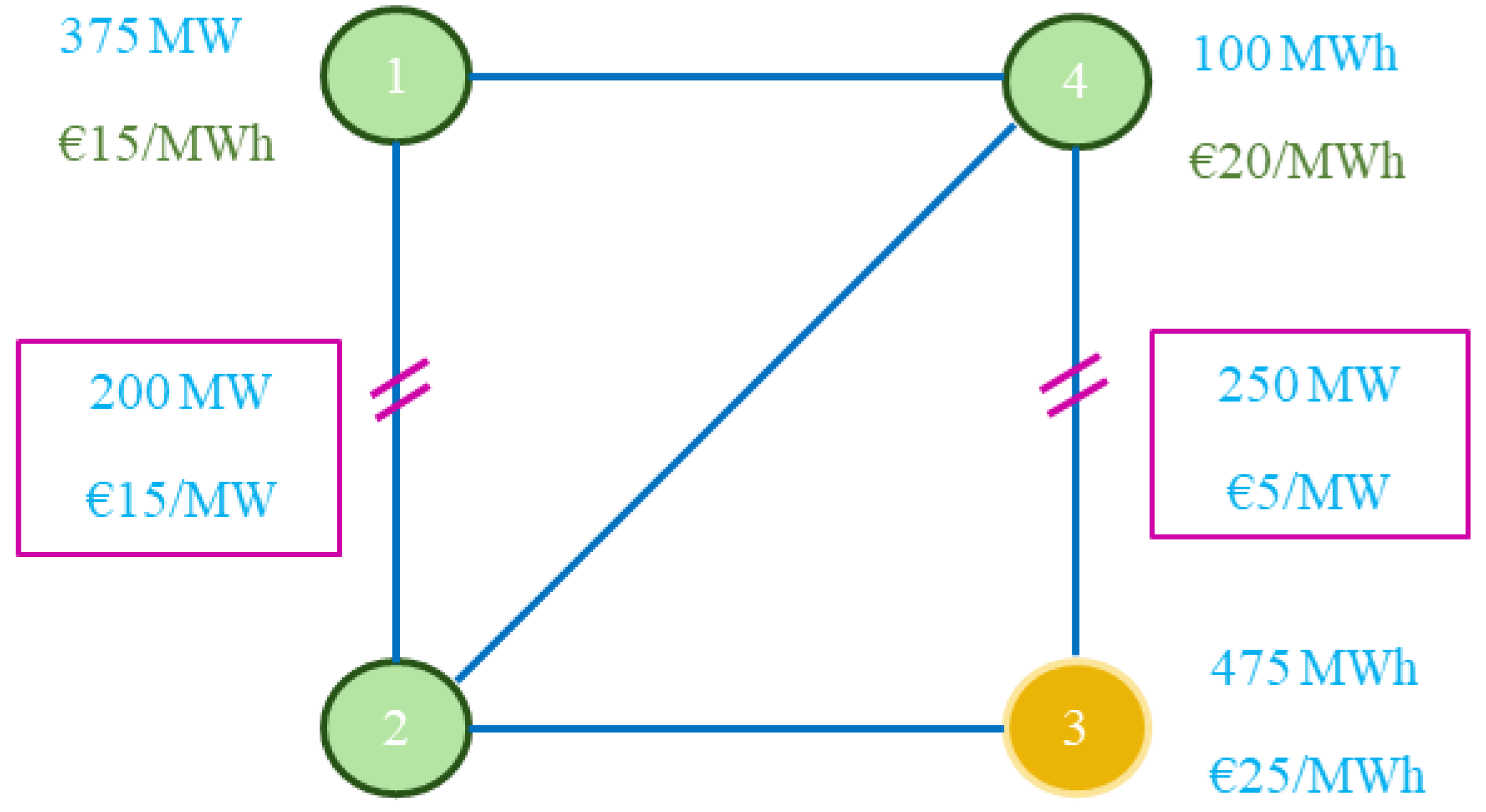
Figure 1. A four-node network with two capacity-constrained lines.
Energies 17 01923 g001
Figure 2. Temporal and spatial dimensions of JETRA under nodal pricing.
Energies 17 01923 g002
Figure 3. Temporal and spatial dimensions of JETRA under zonal pricing.
Energies 17 01923 g003
Figure 4. Market time frames and responsible institutions under different pricing schemes.
Energies 17 01923 g004
Figure 5. Main components of interconnection network capacity under FBMC.
Energies 17 01923 g005
Figure 6. Scenarios 1 and 2 in the energy purchase bid change from the long-term auction.
Energies 17 01923 g006
Figure 7. Scenarios 3 and 4 in the energy purchase bid change from the long-term auction.
Energies 17 01923 g007
Figure 8. Long-term auction results under nodal pricing.
Energies 17 01923 g008
Figure 9. Real-time dispatch under nodal pricing.
Energies 17 01923 g009
Figure 10. Reference day transaction pattern for the long-term auction.
Energies 17 01923 g010
Figure 11. Base case and reference flow for the long-term auction.
Energies 17 01923 g011
Figure 12. Reference day interzonal transaction pattern for the day-ahead auction.
Energies 17 01923 g012
Figure 13. Base case and reference flow for the day-ahead auction.
Energies 17 01923 g013
Figure 14. Long-term auction outcomes under zonal pricing.
Energies 17 01923 g014
Figure 15. Day-ahead market clearing results under zonal pricing.
Energies 17 01923 g015
Figure 16. National-based redispatch results.
Energies 17 01923 g016
Figure 17. Cross-border redispatch results.
Energies 17 01923 g017
Figure 18. Ex-ante GDSK comparison with optimal values.
Energies 17 01923 g018
Table 1. Five bids in the case study for JETRA.
Bid ProductsLocationPrice (€/MWh)Volume Lower Boundary (MW)Volume Higher Boundary
(MW)
Bid 1FTRInjection at node 1 (zone west) and withdrawal at node 3 (zone east)10200500
Bid 2Energy saleInjection at node 2800150
Bid 3Energy saleInjection at node 4200300
Bid 4PTRInterconnection between node 1 and node 2100150
Bid 5Energy purchaseWithdrawal at node 3250300
Table 2. Process and computation at different timesteps for JETRA implementation.
Time StepReal-World Process for TSOs and Power ExchangeComputation Process
Before the long-term auction
  • Anticipation of market outcomes several years before electricity delivery
  • Construction of the grid model using the best estimate of the system state
  • Selection of the base case for long-term auction
  • Derivation of the reference flow from the base case
  • Selection of the GDSK (In this research, we consider the generation and demand change in relation to the net import or export. Therefore, we expand the GSK concept in the FBMC to the generation demand shift keys (GDSKs)) and the flow reliability margin
  • Calculation of the main grid parameters: zonal PTDF and RAM
On the day of the long-term auction
  • Submissions of supply and purchase bids from market players to power exchanges
  • Market clearing using the JETRA algorithm
D-2
  • Anticipation of market outcome two days before electricity delivery
  • Construction of the grid model using the best estimate of the system state
  • Selection of the base case for the day-ahead auction
  • Derivation of the reference flow from the base case
  • Selection of the GDSK and the flow reliability margin
  • Calculation of the main grid parameters: zonal PTDF and RAM
D-1
  • Submissions of supply and purchase bids from market players to power exchanges
  • Market clearing using the JETRA algorithm
D
  • Assessment of grid feasibility
  • Redispatch
  • Nodal optimal power flow in the national or cross-border redispatch
Table 3. β values of each bid in nodal pricing for each network element.
Capacity
(MW)
Bid 1Bid 2Bid 3Bid 4Bid 5Shadow Price (€/MW)
Line 1–22000.5−0.1250.1251015
Line 2–1200−0.50.125−0.125−100
Line 1–44000.50.125−0.125000
Line 4–1400−0.5−0.1250.125000
Line 2–34000.50.6250.375000
Line 3–2400−0.5−0.625−0.375000
Line 2–440000.25−0.25000
Line 4–24000−0.250.25000
Line 3–4250−0.5−0.375−0.625000
Line 4–32500.50.3750.625005
Table 4. Payment from bid winners to the SO in the long-term auction under nodal pricing.
Bidder 1Bidder 2Bidder 3Bidder 4Bidder 5
TypeFinancial Transmission RightsEnergy SaleEnergy SalePhysical Transmission RightsEnergy Purchase
Upper bound (MW)500150300100300
Lower bound (MW)2000000
Bid price (€/MWh)1080201025
Result quantity (MWh)37501000100
Result price (€/MW)10020025
Payment to SO (€)37500−200002500
Table 5. Payment from SO to previous round bid winners in the day-ahead market.
Bidder 1Bidder 2Bidder 3Bidder 4Bidder 5
TypeFinancial Transmission RightsEnergy SaleEnergy SalePhysical Transmission RightsEnergy Purchase
Quantity (MW)37501000100
Price (€/MW)1200200135
Payment to SO (€)45,0000−2000013,500
Table 6. RAM and PTDF of bidders in the long-term auction under zonal pricing.
Capacity Limit
(MW)
PTDF
Bid 1
PTDF
Bid 2
PTDF
Bid 3
PTDF
Bid 4
PTDF
Bid 5
Line 1–2122.50.56250010
Line 2–1197.5−0.56250000
Line 1–44000.43750000
Line 4–1400−0.43750000
Table 7. Payments from bid winners to the SO in long-term auctioning.
Bidder 1Bidder 2Bidder 3Bidder 4Bidder 5
TypeFinancial Transmission RightsEnergy SaleEnergy SalePhysical Transmission RightsEnergy Purchase
Upper bound (MW)500150300100300
Lower bound (MW)2000000
Bid price (€/MW)1035201025
Quantity217.7703000300
Price (€/MW)10025025
Payment to SO (€)21780−750007500
Table 8. RAM and Zonal PTDF values in day-ahead market clearing.
Capacity
(MW)
PTDF
Bid 1
PTDF
Bid 2
PTDF
Bid 3
PTDF
Bid 5
Shadow Price (€/MW)
Line 1–2158.750.550009.09
Line 2–1221.25−0.550000
Line 1–44000.450000
Line 4–1400−0.450000
Table 9. Generation and load payments to the SO in the day-ahead market.
TypeGenerationGenerationGenerationLoad
ZoneZone WestZone EastZone EastZone East
Quantity (MW)288.60211.4500
Price (€/MW)1502020
Payment to SO (€)43290422810,000
Table 10. Payments from the SO to bid winners in the long-term market.
Bidder 1Bidder 2Bidder 3Bidder 4Bidder 5
TypeFinancial Transmission RightsEnergy SaleEnergy SalePhysical Transmission RightsEnergy Purchase
Quantity (MW)217.803000300
Price (€/MW)5020020
Payment to SO (€)10890600006000
Table 11. Payments from SO to generators in national-based redispatch.
Generator 2Generator 4
Redispatch type+ (Generation increase)− (Generation decrease)
Volume (MW)105.6105.6
Net payment from SO to generator (€)84480
Table 12. Payments from the SO to generators in cross-border redispatch.
Generator 1Generator 2Generator 4
Redispatch type+ (Generation
increase)
+ (Generation
increase)
− (Generation
decrease)
Volume (MW)111.450161.4
Net payment from SO to generator (€)167140000
Table 13. Total cost for the user at demand node 3 under nodal and zonal pricing.
Nodal Pricing (€)Under National Redispatch (€)Under Cross-Border Redispatch (€)
15,25021,03718,260
Table 14. GDSK metric for different timeframes.
Optimal GDSK in Zone East among Nodes 2, 3, and 4Ex-Ante GDSK in Zone East among Nodes 2, 3, and 4Euclidean Distance between the Ex-Ante and Optimal ValuesRealized GDSK in Zone East among Nodes 2, 3, and 4
Long-term auction(0, 0.47, 0.53)(0.5, 0.5, 0)0.729(0, 1, 0)
Day-ahead/Real-time market(−0.125, 0.625, 0.5)(0.4, 0.6, 0)0.725(0, 0.866, 0.134)
Table 15. GDSK for national-based and cross-border redispatch.
Ex-Post GDSKOptimal GDSK for Day-Ahead MarketEuclidean Distance
National redispatch(−0.366, 0.866, 0.5)(−0.125, 0.625, 0.5)0.34
Cross-border redispatch(−0.125, 0.625, 0.5)(−0.125, 0.625, 0.5)0
Table 16. Cross-border FTR in long-term and day-ahead auctions.
Cross-Border FTR
Nodal Pricing (MWh)
Cross-Border Trade Zonal Pricing (MWh)Potential Optimal Interzonal Transaction Zonal Pricing (MWh)Interconnection Utilization Rate under Zonal Pricing (%)
Long-term auction375217.8282.373.2
Day-ahead/real-time market400288.637885.4
Table 17. Balance with the SO.
SO Surplus from Generation Load Payment in Day-Ahead Market (€)SO Payment to Long-Term Right Holders (€)SO Balance after
Day-Ahead Market (€)
National-Based Redispatch Costs (€)Cross-Border Redispatch Costs
(€)
1443108935484485671
Disclaimer/Publisher’s Note: The statements, opinions and data contained in all publications are solely those of the individual author(s) and contributor(s) and not of MDPI and/or the editor(s). MDPI and/or the editor(s) disclaim responsibility for any injury to people or property resulting from any ideas, methods, instructions or products referred to in the content.

