A Model Predictive Control Strategy with Minimum Model Error Kalman Filter Observer for HMEV-AS

Abstract

In hub-motor electric vehicles (HMEVs), performance is adversely affected by the mechanical-electromagnetic coupling effect arising from deformations of the air gap in the Permanent Magnet Brushless Direct Current Motor (PM BLDC), which are exacerbated by varying road conditions. In this paper, a Model Predictive Control (MPC) strategy for HMEVs equipped with air suspension (AS) is introduced to enhance ride comfort. Firstly, an 18-degree of freedom (DOF) full-vehicle model incorporating unbalanced electromagnetic forces (UEMFs) induced by motor eccentricities is developed and experimentally validated. Additionally, a Minimum Model Error Extended Kalman Filter (MME-EKF) observer is designed to estimate unmeasurable state variables and account for errors resulting from sprung mass variations. To further improve vehicle performance, the MPC optimization objective is formulated by considering the suspension damping force and dynamic displacement constraints, solving for the optimal suspension force within a rolling time domain. Simulation results demonstrate that the proposed MPC approach significantly improves ride comfort, effectively mitigates coupling effects in hub driving motors, and ensures that suspension dynamic stroke adheres to safety criteria. Comparative analyses indicate that the MPC controller outperforms conventional PID control, achieving substantial reductions of approximately 41.59% in sprung mass vertical acceleration, 14.29% in motor eccentricity, 1.78% in tire dynamic load, 17.65% in roll angular acceleration, and 16.67% in pitch angular acceleration.

1. Introduction

Increasing concerns about global warming, climate change, and fuel shortages make it essential for future transportation systems to focus on sustainability and efficiency [1,2]. It should be emphasized that the environmental benefits of electric vehicles are crucially dependent on the ecological sourcing of electricity. Studies indicate that when battery charging relies on renewable energy systems such as wind, hydro, and solar power, electric vehicles can achieve over 60% greater lifecycle emission reductions compared to conventional internal combustion engine vehicles [3]. The hub-motor driving electric vehicles (HMEVs) are increasingly recognized as an effective solution to mitigate environmental pollution stemming from excessive engine emissions [4], particularly when integrated with clean energy infrastructure. Furthermore, numerous advantages are offered by HMEVs as a common propulsion setup for electric vehicles. These advantages include a simplified transmission system, accurate and rapid independent control of torque for each hub motor, and the ease of vehicle light weighting technology [5,6,7]. However, technical challenges arise from placing the motor in the wheel, as it increases the unsprung mass, which could negatively impact vehicle dynamic performances [8]. Moreover, the unbalance electromagnetic force (UEMF) produced by deformations in the magnetic gap due to road excitations compromise ride comfort [9].

To alleviate the above detrimental impacts, it is suggested to introduce a suspension system to HMEVs. The vehicle suspension, a vital element of the chassis system, effectively buffers the impact from road roughness and plays a critical role in delivering outstanding ride comfort to passengers. However, the parameters of the passive suspension are non-adjustable, limiting its ability to achieve optimal vibration suppression across varying road conditions [10]. Li et al. presented an analysis of the dynamic characteristics of a hub direct drive-air suspension system, focusing on the vertical and longitudinal directions, to address issues related to vibration and stability in hub-motor electric vehicles [11]. Omer Bingül et al. researched the application of the Non-dominated Sorting Genetic Algorithm II to address multi-objective optimization challenges in a 4 × 4 wheel-motor-driven electric vehicle equipped with a nonlinear active suspension system [12]. Dal-Seong Yoon et al. designed a semi-active magnetorheological damper suspension system controller using direct and indirect adaptive sliding mode control methods, thereby enhancing HM-EV performance in terms of vibration control and ride comfort [13]. Olivier Munyaneza et al. introduced a novel hybrid annular radial magneto-rheological damper to enhance the ride comfort of electric vehicles driven using hub motors [14]. Wu Hang et al. proposed a particle swarm optimization algorithm that is applied to multi-objective optimization in active suspension systems to counteract negative coupling effects [15]. However, HMEVs with active suspension are confronted with continuous disturbances and result in high energy consumption and costs, which could hinder market adoption. In contrast, semi-active suspension offers lower energy consumption and cost-effective features. With appropriate control strategies, HMEVs with semi-active suspension provide high performance. A. Alonso et al. introduced an adaptive air suspension system with an LQR control strategy. Experimental results indicated that the suspension system employing the adaptive algorithm reduced the sprung mass acceleration by 30% compared to passive suspension [16]. A fuzzy sliding mode controller (FSMC) was developed to improve the precision of body height adjustment and minimize the peak values of body roll and pitch angles. The reliability of the controller was validated through bus experiments [17]. Gang Li et al. employed fuzzy control to adjust the boundary layer of sliding mode control, effectively suppressing the influence on the control precision of semi-active air suspension and ensuring system stability [18]. However, LQR and fuzzy control typically lack the ability to handle constraints effectively [19,20]. MPC has gained popularity for its straight-forward design, ease of implementation, and robustness against parameter uncertainties. Moreover, MPC process physical constraints within the control domain and predict future dynamics through a predictive model, thus optimizing current and predictive states.

In response to these obstacles, the investigation presented a damping control approach tailored for the HMEVs featuring a semi-active suspension system. The primary goals were to enhance ride comfort, bolster handling stability, and diminish the disparity between the stator and rotor. The key contributions of this research are as follows: (1) development of a cooperative system integrating HMEV and air suspension as HMEV equipped air suspension (HMEV-AS); (2) an MPC controller considering constraints is designed to mitigate vibration and eccentricity to obtain a significant reduction in vehicle body acceleration and pitch angular acceleration, respectively; (3) an MME-EKF observer is also devised to capture the necessary state variables for the MPC controller, factoring in errors from state variables induced by changes in sprung mass.

The paper is structured as follows: the electromechanical coupling model is developed and preliminary insights into the UEMF are provided in Section 2. The verification of the HMEV-AS dynamic model through testing is provided in Section 3. The design of the MPC controller is presented in Section 4. Simulation outcomes are summarized in Section 5. Finally, key conclusions are drawn in Section 6.

2. HMEV-AS Model

This study focused on developing a model for HMEV-AS, consisting of the following four primary elements: a hub-motor model that produces an UEMF impacting both the wheels and suspension system; linear air suspension model, which was used to calculate damping force; a full-vehicle dynamics model, which focused on the response of the vehicle to dynamic conditions; and a road excitation model, which introduced external forces to the system.

2.1. Hub-Motor Model

The PM BLDC motor offers benefits such as high transmission efficiency, a compact design, and low noise levels. The three-phase winding is star-shaped and six-state in the PM BLDC motor, the circuit equation is written as follows [21]:

$${\left[\begin{array}{c}{U}_1 U_2\end{array} U_3\right]}^{\mathrm{T}}={\displaystyle \frac{\mathrm{d}}{\mathrm{d}t}}diag[\begin{array}{c}{L}_1 L_2\end{array} L_3]p{\left[\begin{array}{c}\begin{array}{c}{i}_1 i_2\end{array} i_3\end{array}\right]}^{\mathrm{T}}+diag[\begin{array}{c}{R}_1 R_2\end{array} R_3]{\left[\begin{array}{c}\begin{array}{c}{i}_1 i_2\end{array} i_3\end{array}\right]}^{\mathrm{T}}+{\left[\begin{array}{c}\begin{array}{c}{e}_1 e_2\end{array} e_3\end{array}\right]}^{\mathrm{T}}$$

(1)

in which U₁, U₂, U₃ is A-phase, B-phase, C-phase winding voltages, L₁, L₂, L₃ is A-phase, B-phase, C-phase winding inductance, p is the differential operator, i₁, i₂, i₃ is A-phase, B-phase, C-phase winding phase current, R₁, R₂, R₃ is A-phase, B-phase, C-phase winding phase resistance, e₁, e₂, e₃ is A-phase, B-phase, C-phase winding back electromotive forces.

The electromagnetic torque of PM BLDC represents as follows:

$$J{\displaystyle \frac{\mathrm{d}{\omega }_{\mathrm{r}}}{\mathrm{d}t}}+B{\omega }_{\mathrm{r}}=T_{\mathrm{e}}-T_{\mathrm{L}}$$

(2)

$$T_{\mathrm{e}}={\displaystyle \frac{1}{{\omega }_{\mathrm{r}}}}(e_{\mathrm{a}}{I}_{\mathrm{a}}+e_{\mathrm{b}}{I}_{\mathrm{b}}+e_{\mathrm{c}}{I}_{\mathrm{c}})$$

(3)

in which T_e is motor electromagnetic torque, J is moment of inertia in motor, B is friction coefficient, T_L is load torque in motor, ω_r represents motor angular velocity.

2.2. Unbalance Magnetic Pull

In a PM BLDC motor, the magnetic field in the air gap is influenced by both the permanent magnets and the armature reaction. By employing the linear superposition method, the radial and tangential magnetic fields were calculated across the air gap of the motor. Figure 1 shows PM BLDC, highlighting the air gap eccentricity to assist in computing the UEMFs. The radial air gap magnetic field in the eccentric state B_er and radial magnetic field of the permanent magnet B_mr are as follows [22]:

$$B_{\mathrm{er}}\left(r,\beta ,t\right)=\left[B_{\mathrm{mr}}\left(r,\beta ,t\right)+B_{\mathrm{ar}}\left(r,\beta ,t\right)\right]{\epsilon }_{\xi }$$

(4)

$$B_{\mathrm{et}}\left(r,\beta ,t\right)=\left[B_{\mathrm{mt}}\left(r,\beta ,t\right)+B_{\mathrm{at}}\left(r,\beta ,t\right)\right]{\epsilon }_{\xi }$$

(5)

where F_ez is vertical UEMF and F_ex is longitudinal UEMF, r is radius, L is the axial length of the motor, and λ₀ is vacuum permeability.

The main specification of the PM BLDCM model is illustrated in

Table 1. Structure parameters of hub motor.

Parameters	Value	Unit	Parameters	Symbol	Value	Unit
Winding turns Ns	24	-	Radius of permanent magnet position	Rm	0.1008	m
Slot number Qs	51	-	Permanent magnet thickness	hm	0.0025	m
Parallel branches of winding number a	1	-	Axial length of motor	L	0.06	m
Slot width b0	0.00214	m	Permanent magnet remanence	Br	1.33	T
Slot angle α0	0.0214	rad	Winding pitch	αy	1	rad
Outer radius of stator Rs	0.1	m	Polar arc coefficient	αp	1	-
Inner radius Rr	0.1033	m	Pole pairs	p	23	-
Relative recovery permeability μr	1.1	-	Initial angle of stator to rotor	θ0	0	rad
Single-phase winding number N	17	-	Vacuum permeability	μ0	4π × 10−7	N/A2

.

2.3. Linear Air Suspension Model

The air spring force F_spr is written as follows:

$$F_{\mathrm{s}\mathrm{p}\mathrm{r}}=(P-P_{\mathrm{a}})A_{\mathrm{e}}$$

(6)

$$A_{\mathrm{e}}=A_0+D_{\mathrm{s}\mathrm{e}}{f}_{\mathrm{d}}$$

(7)

where P is pressure, P_a is atmospheric pressure, A_e is effective area, A₀ is initial sectional area of air spring, D_se is change rate of effective area in air spring, and f_d is suspension deflection.

Linearization in MPC significantly simplifies the computational demands, which is crucial for real-time applications. Additionally, a linear model allows for a more straightforward and intuitive prediction of the future system, simplifying the optimization problem typically involved in MPC. For MPC controller design, the air suspension model is linearized.

The volume and effective cross-sectional area of the air spring change linearly with the height of the spring when the amplitude is low, and the coefficient k_s is calculated as follows [23]:

$$k_{\mathrm{s}}=-D_{\mathrm{s}\mathrm{e}}\left(P_0-P_{\mathrm{a}}\right)+D_{\mathrm{v}\mathrm{e}}{\displaystyle \frac{k{P}_0{A}_0}{V_0}}$$

(8)

where P₀, A₀, and V₀ are the initial pressure, area, and volume, respectively.

The linearization air spring force is

$$F_{\mathrm{s}\mathrm{p}\mathrm{r}}=k_{\mathrm{s}}{f}_{\mathrm{d}}$$

(9)

Figure 2 demonstrates the variation of the effective area A as a function of suspension deflection. A and h are fitted into Equation (10).

$$A\left(h\right)=-1.725\times {10}^{-2}h+0.0089$$

(10)

in which A is the effective area of air suspension, h is suspension deflection, and D_se is −1.725 × 10⁻² m²/m, obtained through calculation.

Dampers, as crucial elements of the suspension system, play an integral role in enhancing vehicle ride smoothness and handling stability. Traditional dampers, however, have a fixed damping coefficient, which limits their ability to adapt to varying operational conditions. In this study, a controllable damper was applied in the suspension system.

The force exerted by this controllable damper is denoted as F_c, which can be modelled as a function of the control current i and the relative velocity between the suspension deflection [24].

$$F_{\mathrm{c}}=A\left(i\right)S_{\mathrm{b}}{\dot{f}}_{\mathrm{d}}$$

(11)

The polynomial function employed in the adjustable damper is

$$A_{\mathrm{d}}(i)={\sum }_{n=0}^k{a}_{\mathrm{n}}{i}^n$$

(12)

where A_d(i) is the function of the control current i determines the maximum damping force achievable with the applied current at the highest excitation velocity, a_n is polynomial coefficient, and n is polynomial degree.

The shape function, which describes the shape relationship between the damping force and the relative velocity, is written as follows:

$$S_{\mathrm{b}}\left({\dot{f}}_d\right)=\mathrm{s}\mathrm{g}\mathrm{n}\left({\dot{f}}_{\mathrm{d}}\right)[1-\mathrm{e}\mathrm{x}\mathrm{p}(-{\displaystyle \frac{b_0\left|{\dot{f}}_{\mathrm{d}}\right|}{C}})]$$

(13)

The specifications of the adjustable damping damper are shown in

Table 2. Specifications of adjustable damper.

$\mathbf{Stretching} \mathbf{Stroke} {\dot{\mathit{f}}}_{\mathbf{d}}\ge 0$		$\mathbf{Compression} \mathbf{Stroke} {\dot{\mathit{f}}}_{\mathbf{d}}<0$
a0  +	4002.72	a0  −	−2002.45
a1  +	−1567.91	a1  −	801.58
b0  +	3.41	b0  −	9.48
C  +	1.31	C  −	3.38

“⁺” of superscript represents stretching stroke; “⁻” of superscript represents compression stroke.

.

2.4. Dynamic Model

To investigate the dynamic performance of the HMEV-AS system under road excitation, a quarter-vehicle system dynamic model is first established by integrating the tire model, air spring model, and adjustable damper model. This quarter-vehicle model accounts for the relative displacement between the stator core and rotor core inside the hub motor. The hub motor is divided into two components at the bearing interface: the stator core and the rotor core. Based on the tire ring model theory, the quarter-vehicle system is decomposed into four mass blocks: sprung mass, stator mass, wheel and rotor mass, and tire ring mass as shown in Figure 3.

The dynamic model of the full vehicle is simplified to 18 degrees of freedom: 12 vertical motions of unsprung mass; roll; pitch; yaw and lateral motions; and vertical and longitudinal motions of sprung mass. The simplified physical model is shown in Figure 4.

In Figure 4, M_b—mass of sprung mass, M_ti—mass of tire ring unit, M_{ω_mri}—mass of wheel and rotor assembly, M_msi—mass associated with the stator assembly and its attachments, F_spri—suspension-restoring force, c_i—suspension damping rate, F_ezi is vertical electromagnetic force, q_i—road surface displacement input, z_si—sprung mass vertical displacement, z_ti—vertical displacement input, z_{ω_mri}—vertical movement of wheel–rotor set, z _msi—vertical position of stator assembly, k_beazi—stiffness of the motor hub bearing, parameters a and b—longtudinal distances from sprung mass center to front/rear wheel to centers, B_r and B_f—the rear and front track widths, respectively.

Vertical motion for sprung mass is written as follows:

$$m_{\mathrm{b}}{\ddot{z}}_{\mathrm{b}}=-{\sum }_{i=1}^4{F}_{\mathrm{spri}}-{\sum }_{i=1}^4{c}_{\mathrm{i}}\left({\dot{z}}_{\mathrm{si}}-{\dot{z}}_{\mathrm{msi}}\right)\begin{array}{c}(i=1, 2, 3, 4)\end{array}$$

(14)

Roll motion for the sprung mass is

$$I_{\mathrm{x}}\ddot{\phi }=\left[F_{\mathrm{spr}1}+c_1\left({\dot{z}}_{\mathrm{s}1}-{\dot{z}}_{\mathrm{ms}1}\right)\right]\cdot {\displaystyle \frac{B_{\mathrm{f}}}{2}}+\left[F_{\mathrm{spr}3}+c_3\left({\dot{z}}_{\mathrm{s}3}-{\dot{z}}_{\mathrm{ms}3}\right)\right]\cdot {\displaystyle \frac{B_{\mathrm{r}}}{2}}$$

$$-\left[F_{\mathrm{spr}2}+c_2\left({\dot{z}}_{\mathrm{s}2}-{\dot{z}}_{\mathrm{ms}2}\right)\right]\cdot {\displaystyle \frac{B_{\mathrm{f}}}{2}}-\left[F_{\mathrm{spr}4}+c_4\left({\dot{z}}_{\mathrm{s}4}-{\dot{z}}_{\mathrm{ms}4}\right)\right]\cdot {\displaystyle \frac{B_{\mathrm{r}}}{2}}-h_{\mathrm{g}}\cdot {\sum }_{i=1}^4{F}_{\mathrm{yi}}$$

(15)

Pitch motion for the sprung mass is

$$I_{\mathrm{y}}{\ddot{\theta }}_{\mathrm{b}}=-\left[F_{\mathrm{spr}1}-c_1\left({\dot{z}}_{\mathrm{s}1}-{\dot{z}}_{\mathrm{ms}1}\right)\right]\cdot a+\left[F_{\mathrm{spr}3}-c_3\left({\dot{z}}_{\mathrm{s}3}-{\dot{z}}_{\mathrm{ms}3}\right)\right]\cdot b$$

$$-\left[F_{\mathrm{spr}2}-c_2\left({\dot{z}}_{\mathrm{s}2}-{\dot{z}}_{\mathrm{ms}2}\right)\right]\cdot a-\left[F_{\mathrm{spr}4}-c_4\left({\dot{z}}_{\mathrm{s}4}-{\dot{z}}_{\mathrm{ms}4}\right)\right]\cdot b$$

$$-h_{\mathrm{g}}\left({\sum }_{i=1}^4{F}_{\mathrm{ti}}-{\sum }_{i=1}^4{F}_{\mathrm{Ri}}\right)-F_{\mathrm{w}}(h_{\mathrm{w}}-h_{\mathrm{g}})$$

(16)

Longitudinal motion is

$$[M_{\mathrm{b}}+{\sum }_{i=1}^4\left(M_{\mathrm{m}\mathrm{s}\mathrm{i}}+M_{{\mathsf{\omega }}_{\mathrm{m}\mathrm{r}\mathrm{i}}}+M_{\mathrm{t}\mathrm{i}}\right)]{\dot{u}}_{\mathrm{a}}={\sum }_{i=1}^4{F}_{\mathrm{t}\mathrm{i}}-{\sum }_{i=1}^4{F}_{\mathrm{R}\mathrm{i}}-F_{\mathrm{w}}$$

(17)

Lateral motion is

$$[M_{\mathrm{b}}+{\sum }_{i=1}^4\left(M_{\mathrm{m}\mathrm{s}\mathrm{i}}+M_{{\mathsf{\omega }}_{\mathrm{m}\mathrm{r}\mathrm{i}}}+M_{\mathrm{t}\mathrm{i}}\right)]\ddot{y}={\sum }_{i=1}^4{F}_{\mathrm{y}\mathrm{i}}$$

(18)

Vertical motion for total mass of hub-motor stator and its related accessories

$$m_{\mathrm{msi}}{\ddot{z}}_{\mathrm{msi}}-F_{\mathrm{spri}}-c_{\mathrm{si}}\left({\dot{z}}_{\mathrm{si}}-{\dot{z}}_{\mathrm{msi}}\right)+k_{\mathrm{beazi}}\left(z_{\mathrm{msi}}-z_{\mathrm{w}\_\mathrm{mri}}\right)-F_{\mathrm{ezi}}=0\begin{array}{c} (i=1, 2, 3, 4)\end{array}$$

(19)

Vertical motion for mass of hub motor rotor and the wheel rim

$$\begin{gathered} m_{\mathrm{w}\_\mathrm{mr}\mathrm{i}}{\ddot{z}}_{\mathrm{w}\_\mathrm{mr}\mathrm{i}}-k_{\mathrm{beazi}}\left(z_{\mathrm{msi}}-z_{\mathrm{w}\_\mathrm{mr}\mathrm{i}}\right)+k_{\mathrm{t}\_\mathrm{rdi}}\left(z_{\mathrm{w}\_\mathrm{mr}\mathrm{i}}-z_{\mathrm{ti}}\right) \\ +c_{\mathrm{t}\_\mathrm{rdi}}\left({\dot{z}}_{\mathrm{w}\_\mathrm{mri}}-{\dot{z}}_{\mathrm{ti}}\right)+F_{\mathrm{ezi}}=0\begin{array}{c} (i=1, 2, 3, 4)\end{array} \end{gathered}$$

(20)

Vertical motion for the tire ring

$$\begin{gathered} m_{\mathrm{ti}}{\ddot{z}}_{\mathrm{ti}}-k_{\mathrm{t}\_\mathrm{rdi}}\left(z_{\mathrm{w}\_\mathrm{mr}i}-z_{\mathrm{ti}}\right)-c_{\mathrm{t}\_\mathrm{rdi}}\left({\dot{z}}_{\mathrm{w}\_\mathrm{mri}}-{\dot{z}}_{\mathrm{ti}}\right) \\ +k_{\mathrm{czi}}\left(z_{\mathrm{ti}}-q_i\right)=0 \begin{array}{c}(i=1, 2, 3, 4)\end{array} \end{gathered}$$

(21)

Vertical motion at each suspension and body connection position is as follows:

$$\left\{\begin{array}{c}{z}_{\mathrm{s}1}=zb-a\theta +{\displaystyle \frac{B_{\mathrm{f}}}{2}}\phi \\ z_{\mathrm{s}2}=zb-a\theta -{\displaystyle \frac{B_{\mathrm{f}}}{2}}\phi \\ z_{\mathrm{s}3}=zb+b\theta +{\displaystyle \frac{B_{\mathrm{r}}}{2}}\phi \\ z_{\mathrm{s}4}=zb+b\theta -{\displaystyle \frac{B_{\mathrm{r}}}{2}}\phi \end{array}\right.$$

(22)

The specifications of the HMEV-AS system are shown in

Table 3. Specifications of the HMAS-EV system.

Specifications	Value
Mb (kg)	710
Mω_mri (kg)	20
Mmsi (kg)	30.4
Mti (kg)	34.4
Br (m)	1.55
r (m)	0.245
lf (m)	0.795
lr (m)	0.975
U (V)	72
Kt (kN/s)	260

.

2.5. Road Excitation Model

The frequency domain velocity power spectral density of the road is as follows [25]:

$$G_{\mathrm{v}}\left(n\right)=4{\pi }^2{n}_0^2{G}_q\left(n_0\right)v$$

(23)

where n₀ is the reference spatial frequency, n₀ = 0.1 m⁻¹, G_q(n₀) = 64 × 10⁻⁶ m³ at C-class road, and v is vehicle velocity.

It is pertinent to generate time–domain signals of the road by filtering white noise. The filter is constructed as follows:

$$H\left(s\right)={\displaystyle \frac{2\pi \sqrt{G_q\left(n_0\right)v}}{s+2\pi f_0}}$$

(24)

where f₀ is low cutoff frequency, f₀ = 0.01 Hz. The time–domain signal of the road is

$$\dot{q}\left(t\right)=-2\pi f_{0}q\left(t\right)+2\pi \sqrt{G_{\mathrm{q}}\left(n_0\right)v}w\left(t\right)$$

(25)

where w(t) is white noise.

Equation (26) is the front-left road excitation, Equation (26) is the coherence function, and the front-right road excitation is calculated as follows:

$$\gamma \left(n,T_{\mathrm{w}}\right)={\left[1+{\left({\displaystyle \frac{n{T_{\mathrm{w}}}^a}{n_0}}\right)}^W\right]}^{-p}$$

(26)

where T_w is track width, p is a reference factor, and a is the constant index of track width T_w.

For the given excitation q₁(t) and q₂(t) on the left and right wheel, the transfer function G(s) can be written as follows [26]:

$$G\left(s\right)={\displaystyle \frac{Q_2\left(s\right)}{Q_1\left(s\right)}}={\displaystyle \frac{a_0+a_{1}s+a_2{s}^2\cdots }{b_0+b_{1}s+b_2{s}^2\cdots }}$$

(27)

where Q₁(s) and Q₂(s) are the LaPlace transform of q₁(t) and q₂(t). Combined with (23) and (27),

$$\left|G\left(s\right)\right|=\left|\gamma \left(n,T_{\mathrm{w}}\right)\right|$$

(28)

Pade approximation method was used; while retaining the third-order results, genetic algorithms are used to calculate the relevant parameters of the left and right road excitation transfer functions. The specifications are shown in

Table 4. The transfer function parameters of the left-side and right-side roads.

Molecular Coefficient		Denominator Coefficient
$a_0$	406,250	$b_0$	406,249
$a_1$	690,430	$b_1$	750,487
$a_2$	61.0354	$b_2$	102,122

.

As the time lag between the front and rear wheel road excitation, the rear-wheel road excitation is expressed as

$$\left\{\begin{array}{c}{q}_3\left(t\right)=q_1(t-\tau )\\ q_4\left(t\right)=q_2(t-\tau )\end{array}\right.$$

(29)

where t ≥ τ, τ is time lag, which is the quotient of vehicle wheelbase and velocity. Considering that hysteresis is difficult to linearize, transfer functions are considered in the complex domain to describe it. The transfer functions are as follows

$$\left\{\begin{array}{c}{G}_3\left(s\right)={\displaystyle \frac{Q_3\left(s\right)}{Q_1\left(s\right)}}={\displaystyle \frac{1-\frac{\tau }{2}s+\frac{{\tau }^2}{12}{s}^2}{1+\frac{\tau }{2}s+\frac{{\tau }^2}{12}{s}^2}}\\ G_4\left(s\right)={\displaystyle \frac{Q_4\left(s\right)}{Q_2\left(s\right)}}={\displaystyle \frac{1-\frac{\tau }{2}s+\frac{{\tau }^2}{12}{s}^2}{1+\frac{\tau }{2}s+\frac{{\tau }^2}{12}{s}^2}}\end{array}\right.$$

(30)

where Q₁(s), Q₂(s), Q₃(s), and Q₄(s) are, respectively, for road surface incentives; q₁(s), q₂(s), q₃(s), and q₄(s) are for the Laplace transform.

The road excitation on the left and right sides of the rear axle are written as follows:

$$\left\{\begin{array}{c}{q}_3\left(t\right)={\mathcal{L}}^{-1}\left\{G_3\left(s\right)\mathcal{L}\left[q_1\left(t\right)\right]\right\}\\ q_4\left(t\right)={\mathcal{L}}^{-1}\left\{G_4\left(s\right)\mathcal{L}\left[q_2\left(t\right)\right]\right\}\end{array}\right.$$

(31)

3. Experimental Validations

The vehicles were modified to the HMEV-AS configuration to verify the accuracy of the simulation model. The test vehicle and the sensors used for data collection are shown in Figure 5. The HMEV-AS system was created by modifying a Zhidou 1 pure electric vehicle, with parameters shown in

Table 5. Technical specifications of Zotye Zhidou 1.

Specifications	Zotye Zhidou 1
Manufacturer	Zotye Zhidou
Power Type	Pure Electric
Range	120 km (NEDC Standard)
Top speed	80 km/h
Battery Type	Lithium Iron Phosphate (LFP) Battery (10.5 kWh)
Charging Time	Slow Charge: 6 h (0–100%)
	Fast Charge: 20 min (0–80%)
Motor Power	Rated Power: 9 kW, Peak Power: 18 kW

.

As illustrated in Figure 5, PCB acceleration sensors were attached to the front-left sprung mass and the front-left stator position of the vehicle to ensure precise measurements during testing. Figure 6 shows the hub motor-driven vehicle during the test, along with the associated data acquisition equipment and sensors used for performance analysis. In this setup, the test vehicle was equipped with a hub motor that directly drives the wheels, and advanced sensors were employed to monitor the vehicle’s response under controlled conditions.

The vehicle was driven at a constant speed of 30 km/h on a B-level road, in accordance with the national standard for testing in China (GB/T 4970-2009) [27]. The test was performed on a stable surface to ensure the reliability of the results. Data were recorded using the LMS SCADAS Mobile SCR05 system, which continuously collected measurements during the vehicle’s 8-s drive at the specified speed. This arrangement allowed for the precise capture of vehicle dynamics data, particularly with respect to the sprung and unsprung masses under consistent driving conditions.

To compare the test results with the simulation, the power spectral density (PSD) of the collected signals was analysed. This analysis method is used to examine the frequency components of the signals and evaluate the vehicle’s dynamics in response to the hub motor and air suspension system. Figure 6a,b demonstrates that the waveform trends and peak values from the test data closely align with the simulation results, confirming the robustness and reliability of the simulation model when compared to real-world test conditions. The consistency between the power spectral density results further confirms the accuracy of the simulation in reflecting the actual vehicle dynamics observed during the test.

It is concluded that the established model is accurate. A few errors of the HMEV-AS dynamic simulation and test results may arise from external disturbances such as air resistance during the test, and the influence of suspension rubber bushing on the dynamic performance of the system was not considered in the simulation model.

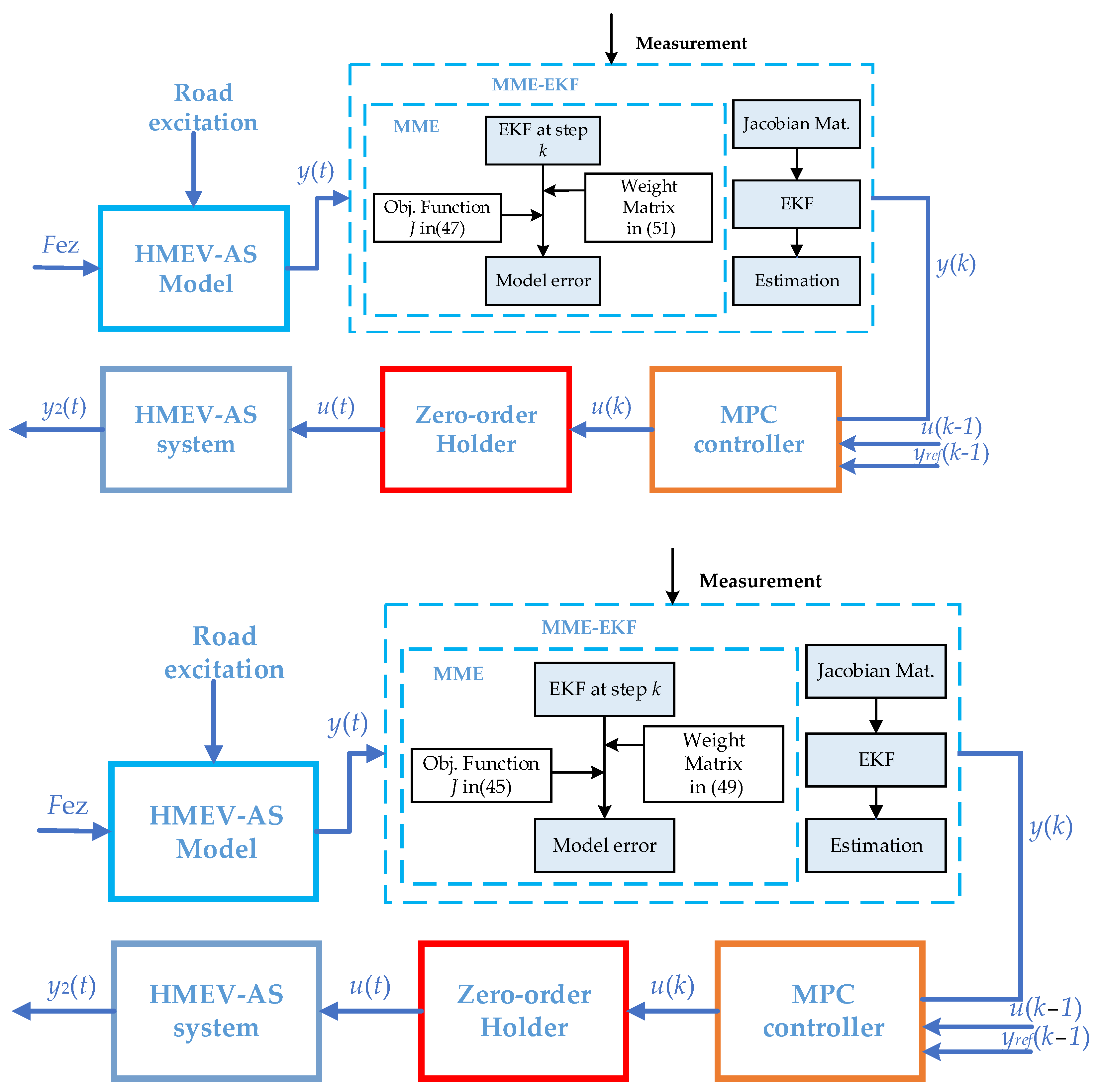
4. MPC Control Design

To enhance the ride comfort of the HMEV-AS system, vehicle body acceleration, pitch angular acceleration, motor eccentricities, and tire dynamic loads are selected as evaluation indicators. Additionally, the damping force generated by the suspension and the limits of suspension dynamic strokes are defined as system constraints within the MPC controller design. To address the issue of state estimation errors due to variations in sprung mass, a Minimum Model Error Extended Kalman Filter (MME-EKF) observer is introduced, enabling the accurate estimation of all necessary system state variables.

As illustrated in Figure 7, the MPC controller flow chart clearly demonstrates the control strategy’s working process: First, road excitation inputs are applied to the established HMEV-AS model to generate initial responses. These outputs, combined with actual measurement data, feed into the MME-EKF module. The MME-EKF module consists of two primary components: the Minimum Model Error (MME) and the Extended Kalman Filter (EKF). Within the MME, an objective function defined in Equation (45) calculates the model error at each step, subsequently adjusting the EKF weight matrix based on Equation (49). Simultaneously, the EKF employs Jacobian matrices to estimate system states accurately. The estimated states are then passed into the MPC controller, along with historical control inputs and reference trajectories, to optimize the control input sequence. The MPC-derived control signals subsequently pass through a zero-order holder to ensure continuous-time signals suitable for actuating the real HMEV-AS system. Finally, the actual controlled outputs of the system are produced, improving ride comfort while adhering strictly to defined suspension performance constraints.

4.1. MPC Controller Design

In linear MPC, the optimization issue is articulated

$$\min J ={\sum }_{\mathrm{k}=1}^{\mathrm{N}}{y}^{\prime }\left(k\right)\mathit{Qy}\left(k\right)+{\sum }_{\mathrm{k}=1}^{\mathrm{N}}{u}^{\prime }\left(k\right)\mathit{Ru}\left(k\right)$$

(32)

$$\mathrm{Subject} \mathrm{to}\left\{\begin{array}{c}x\left(k+1\right)=Ax\left(k\right)+B_{\mathrm{u}}u\left(k\right)\\ y\left(k\right)=Cx\left(k\right)+D_{\mathrm{u}}u\left(k\right)\\ u_{\mathrm{m}\mathrm{i}\mathrm{n}}\le u\left(k\right)\le u_{\mathrm{m}\mathrm{a}\mathrm{x}}\\ x_{\mathrm{m}\mathrm{i}\mathrm{n}}\le x\left(k\right)\le x_{\mathrm{m}\mathrm{a}\mathrm{x}}\end{array}\right.$$

where Q and R represent the respective weighting matrices.

The above-mentioned optimization problem is reformulated into the conventional format of linear quadratic programming.

$$\mathrm{m}\mathrm{i}\mathrm{n}{\displaystyle \frac{1}{2}}{x}^{\mathrm{T}}Gx+f^{\mathrm{T}}x$$

(33)

$$\mathrm{Subject} \mathrm{to} \left\{\begin{array}{c}{A}_{\mathrm{e}}x=b_{\mathrm{e}}\\ A_{\mathrm{j}}x\le b_{\mathrm{j}}\end{array}\right.$$

The linear time-varying state space is

$$\left\{\begin{array}{c}{\dot{x}}_{\mathrm{m}}\left(t\right)=A_{\mathrm{m}}{x}_{\mathrm{m}}\left(t\right)+B_{\mathrm{m}}u\left(t\right)\\ y\left(t\right)=C_{\mathrm{m}}{x}_{\mathrm{m}}\left(t\right)+D_{\mathrm{m}}u\left(t\right)\end{array}\right.$$

(34)

The state matrix is obtained using Jacobi determinant A_m, input matrix B_m, output matrix C_m, and feedforward matrix D_m.

$$\left\{\begin{array}{c}{A}_{\mathrm{m}}={\displaystyle \frac{\partial {\dot{x}}_{\mathrm{m}}}{\partial x_{\mathrm{m}}}}\\ B_{\mathrm{m}}={\displaystyle \frac{\partial {\dot{x}}_{\mathrm{m}}}{\partial u}}\\ C_{\mathrm{m}}={\displaystyle \frac{\partial y}{\partial x_{\mathrm{m}}}}\\ D_{\mathrm{m}}={\displaystyle \frac{\partial y}{\partial u}}\end{array}\right.$$

(35)

The parameters tire ring vertical displacements z_t1, z_t2, z_t3, z_t4, motor stator vertical displacements z_ms1, z_ms2, z_ms3, z_ms4, ring and stator vertical displacements z_{w_mr1}, z_{w_mr2}, z_{w_mr3}, z_{w_mr4}, vehicle body vertical displacement Z_s, roll angle θ, pitch angular φ, and the velocities of the parameters are chosen as state values x_m.

$$\begin{gathered} x_m=[z_{\mathrm{t}1},z_{\mathrm{t}2},z_{\mathrm{t}3},z_{\mathrm{t}\mathrm{r}\mathrm{r}},z_{{\mathrm{w}}_{\mathrm{m}\mathrm{r}1}},z_{\mathrm{w}\_\mathrm{m}\mathrm{r}2},z_{\mathrm{w}\_\mathrm{m}\mathrm{r}3},z_{\mathrm{w}\_\mathrm{m}4},z_{\mathrm{m}\mathrm{s}1}, \\ {z}_{\mathrm{m}\mathrm{s}2},z_{\mathrm{m}\mathrm{s}3},z_{\mathrm{m}\mathrm{s}4},Z_{\mathrm{s}},\theta ,\phi ,{\dot{z}}_{\mathrm{t}1},{\dot{z}}_{\mathrm{t}2},{\dot{z}}_{\mathrm{t}3},{\dot{z}}_{\mathrm{t}4},{\dot{z}}_{\mathrm{w}\_\mathrm{m}\mathrm{r}1},\dot{\theta } \\ {\dot{z}}_{\mathrm{w}\_\mathrm{m}\mathrm{r}2},{\dot{z}}_{\mathrm{w}\_\mathrm{m}\mathrm{r}3},{\dot{z}}_{\mathrm{w}\_\mathrm{m}\mathrm{r}4},{\dot{z}}_{\mathrm{m}\mathrm{s}1},{\dot{z}}_{\mathrm{m}\mathrm{s}2},{\dot{z}}_{\mathrm{m}\mathrm{s}3},{\dot{z}}_{\mathrm{m}\mathrm{s}4},{\dot{Z}}_{\mathrm{s}},\dot{\phi }] \end{gathered}$$

(36)

The suspension control forces F_s1, F_s2, F_s3, and F_s4, four road excitations q₁, q₂, q₃, and q₄; vertical UEMFs F_ez1, F_ez2, F_ez3, and F_ez4 are input vector u. These are the inputs for both the model and the controller.

$$u=[F_{\mathrm{s}1},F_{\mathrm{s}2},F_{\mathrm{s}3},F_{\mathrm{s}4},q_1,q_2,q_3,q_4,F_{\mathrm{e}\mathrm{z}1},F_{\mathrm{e}\mathrm{z}2},F_{\mathrm{e}\mathrm{z}3},F_{\mathrm{e}\mathrm{z}4}]$$

(37)

The vehicle body acceleration ${\ddot{\mathrm{Z}}}_{\mathrm{s}}$, eccentricities of motors e₁, e₂, e₃, and e₄, tire dynamic loads F_d1, F_d2, F_d3, and F_d4, roll angular acceleration $\ddot{\mathsf{\theta }}$, and pitch angular acceleration $\ddot{\mathsf{\phi }}$ are selected as evaluation indicators.

The eccentricities of motors e₁, e₂, e₃, and e₄ are calculated as follows:

$$\left\{\begin{array}{c}{e}_1=z_{\mathrm{m}\mathrm{s}1}-z_{\mathsf{\omega }\_\mathrm{m}\mathrm{r}1}\\ e_2=z_{\mathrm{m}\mathrm{s}2}-z_{\mathsf{\omega }\_\mathrm{m}\mathrm{r}2}\\ e_3=z_{\mathrm{m}\mathrm{s}3}-z_{\mathsf{\omega }\_\mathrm{m}\mathrm{r}3}\\ e_4=z_{\mathrm{m}\mathrm{s}4}-z_{\mathsf{\omega }\_\mathrm{m}\mathrm{r}4}\end{array}\right.$$

(38)

The designer evaluation indexes are taken as the output vector,

$$y=[{\ddot{Z}}_{\mathrm{s}},{e_1,e_2,e}_3,e_4,F_{\mathrm{d}1},F_{\mathrm{d}2},F_{\mathrm{d}3},F_{\mathrm{d}4},\ddot{\theta },\ddot{\phi }]$$

(39)

MPC control strategy is designed by optimizing the evaluation index to improve vehicle performance. The vehicle ride comfort includes vehicle body acceleration, pitch angular acceleration, and roll angular acceleration. Moreover, the eccentricities of the motors are also chosen as the other evaluating indicators of motor vibration, which leads to UEMFs. Moreover, the tire dynamic load indexes the tire earthing ability, which is the evaluating indicator of vehicle handling stability.

$$J(k)={\sum }_{i=1}^p{‖y_{\mathrm{r}\mathrm{e}\mathrm{f}}\left(k+i\left|k\right.\right)-y\left(k+i\left|k\right.\right)‖}_{\mathrm{R}\mathrm{s}}^2+{\sum }_{i=1}^m{‖u\left(k+i\left|k\right.\right)-u\left(k+i-1\left|k\right.\right)‖}_{\mathrm{R}}^2$$

(40)

where reference vector y_ref = [0, 0, 0, 0, 0, 0, 0, 0, 0]^T, R_s is weight coefficient of control target, R is input weight, which is the control cost of controller, and the damping force output has a positive correlation with it; p is prediction step; m is control step.

Using a genetic algorithm to determine the weighting coefficients, first, activate the MPC controller, which already contains a default weighting matrix. Then, generate the initial population. To ensure both speed and accuracy, a population size of 60 is chosen. The system state weighting coefficients and controller inputs are encoded into 20-bit gray codes. Because the state weighting coefficients range from [10e⁰, 10e¹⁰], directly converting them to binary would lead to data loss. Therefore, these coefficients are constrained in exponent form within the range [0, 10]. Meanwhile, the controller input weights are directly converted to binary codes.

$$\left\{\begin{array}{c}F\left(x\right)={\displaystyle \frac{{\mathrm{R}\mathrm{M}\mathrm{S}(\ddot{Z}}_s)}{{{\mathrm{R}\mathrm{M}\mathrm{S}(\ddot{Z}}_s)}_b}}+{\displaystyle \frac{{\mathrm{R}\mathrm{M}\mathrm{S}(e}_3)}{{{\mathrm{R}\mathrm{M}\mathrm{S}(e}_3)}_b}}+{\displaystyle \frac{{\mathrm{R}\mathrm{M}\mathrm{S}(e}_4)}{{{\mathrm{R}\mathrm{M}\mathrm{S}(e}_4)}_b}}\\ +{\displaystyle \frac{{\mathrm{R}\mathrm{M}\mathrm{S}(F}_{d1})}{{{\mathrm{R}\mathrm{M}\mathrm{S}(F}_{d1})}_b}}+{\displaystyle \frac{{\mathrm{R}\mathrm{M}\mathrm{S}(F}_{d2})}{{{\mathrm{R}\mathrm{M}\mathrm{S}(F}_{d2})}_b}}+{\displaystyle \frac{{\mathrm{R}\mathrm{M}\mathrm{S}(F}_{d3})}{{{\mathrm{R}\mathrm{M}\mathrm{S}(F}_{d3})}_b}}\\ +{\displaystyle \frac{{\mathrm{R}\mathrm{M}\mathrm{S}(F}_{d4})}{{{\mathrm{R}\mathrm{M}\mathrm{S}(F}_{d4})}_b}}+{\displaystyle \frac{\mathrm{R}\mathrm{M}\mathrm{S}\left(\ddot{\theta }\right)}{{\mathrm{R}\mathrm{M}\mathrm{S}\left(\ddot{\theta }\right)}_b}}+{\displaystyle \frac{\mathrm{R}\mathrm{M}\mathrm{S}\left(\ddot{\phi }\right)}{{\mathrm{R}\mathrm{M}\mathrm{S}\left(\ddot{\phi }\right)}_b}}\\ x=[r_{s1},r_{s2},r_{s3},r_{s4},r_{s5},r_{s6},r_{s7},r_{s8},r_{s9},r_1]\end{array}\right.$$

(41)

subordinated to

$$\left\{\begin{array}{c}{r}_{s1},\dots ,r_{s9}\in [10e^0,10e^{10}]\\ r_1\in \left[\mathrm{0,1}\right]\\ {\displaystyle \frac{{\mathrm{R}\mathrm{M}\mathrm{S}(\ddot{Z}}_s)}{{{\mathrm{R}\mathrm{M}\mathrm{S}(\ddot{Z}}_s)}_b}}\le 0.8\\ {\displaystyle \frac{{\mathrm{R}\mathrm{M}\mathrm{S}(e}_1)}{{{\mathrm{R}\mathrm{M}\mathrm{S}(e}_1)}_b}}\le 0.8\\ {\displaystyle \frac{{\mathrm{R}\mathrm{M}\mathrm{S}(e}_2)}{{{\mathrm{R}\mathrm{M}\mathrm{S}(e}_2)}_b}}\le 0.8\\ {\displaystyle \frac{{\mathrm{R}\mathrm{M}\mathrm{S}(e}_3)}{{{\mathrm{R}\mathrm{M}\mathrm{S}(e}_3)}_b}}\le 0.8\\ {\displaystyle \frac{{\mathrm{R}\mathrm{M}\mathrm{S}(e}_4)}{{{\mathrm{R}\mathrm{M}\mathrm{S}(e}_4)}_b}}\le 0.8\\ {\displaystyle \frac{{\mathrm{R}\mathrm{M}\mathrm{S}(F}_{d1})}{{{\mathrm{R}\mathrm{M}\mathrm{S}(F}_{d1})}_b}}\le 0.8\\ {\displaystyle \frac{{\mathrm{R}\mathrm{M}\mathrm{S}(F}_{d2})}{{{\mathrm{R}\mathrm{M}\mathrm{S}(F}_{d2})}_b}}\le 0.8\\ {\displaystyle \frac{{\mathrm{R}\mathrm{M}\mathrm{S}(F}_{d3})}{{{\mathrm{R}\mathrm{M}\mathrm{S}(F}_{d3})}_b}}\le 0.8\\ {\displaystyle \frac{{\mathrm{R}\mathrm{M}\mathrm{S}(F}_{d4})}{{{\mathrm{R}\mathrm{M}\mathrm{S}(F}_{d4})}_b}}\le 0.8\\ {\displaystyle \frac{\mathrm{R}\mathrm{M}\mathrm{S}\left(\ddot{\theta }\right)}{{\mathrm{R}\mathrm{M}\mathrm{S}\left(\ddot{\theta }\right)}_b}}\le 0.8\\ {\displaystyle \frac{\mathrm{R}\mathrm{M}\mathrm{S}\left(\ddot{\phi }\right)}{{\mathrm{R}\mathrm{M}\mathrm{S}\left(\ddot{\phi }\right)}_b}}\le 0.8\end{array}\right.$$

(42)

where F(x) is the fitness function, the subscript “b” denotes the default weights of the MPC controller, $r_{s1},\dots ,r_{s11}$ are the state variable weighting coefficients, and $r_1$ is the controller weighting coefficient. The next steps involve selection, crossover, and mutation using a tournament method. In the tournament selection, a certain number of individuals are drawn from the population each time, and the best individual is chosen to enter the offspring population. This process is repeated until the new population size matches the original population size. During crossover and mutation, single-point crossover and uniform mutation are employed, with probabilities of 0.8 and 0.05, respectively. When the number of optimization iterations reaches 200, the termination condition is met. The evaluation metrics after the genetic algorithm (GA) optimization are compared with those before optimization. If the performance is better after optimization, the weight matrix is updated. As shown in Figure 8, the fitness function value decreases significantly after GA optimization, dropping from an initial value from 7.6 to 5.8.

As the suspension has physical limits, the constraint range needs to be set. Considering the damping force provided by the semi-active suspension is opposite to the vertical velocity direction of the suspension, the damping force is calculated.

$$\left\{\begin{array}{c}{0\ge F}_{\mathrm{s}\mathrm{i}}\ge \left(c_{\mathrm{i}\mathrm{m}\mathrm{a}\mathrm{x}}-c_{\mathrm{i}\mathrm{m}\mathrm{i}\mathrm{n}}\right){\dot{f}}_{\mathrm{d}} {\dot{f}}_{\mathrm{d}}\le 0\\ {0\le F}_{\mathrm{s}\mathrm{i}}\le \left(c_{\mathrm{i}\mathrm{m}\mathrm{a}\mathrm{x}}-c_{\mathrm{i}\mathrm{m}\mathrm{i}\mathrm{n}}\right){\dot{f}}_{\mathrm{d}} {\dot{f}}_d>0\end{array}\right.$$

(43)

where c_imin is the minimum of the suspension damping coefficient, and c_imax is the maximum of the suspension damping coefficient.

The suspension stroke displacement is limited,

$$f_{\mathrm{d}\mathrm{c}}\le f_{\mathrm{d}}\le f_{\mathrm{d}\mathrm{r}}$$

(44)

where f_dc is the extreme value of the suspension compression stroke, and f_dr is the extreme value of the suspension rebound stroke. The total suspension travel is ±60 mm, consisting of a 60 mm compression travel and 60 mm extension travel. The travel range will be enforced as a constraint in the MPC controller to ensure the suspension movement remains within the specified limits.

Equation (46) is written in matrix form as follows:

$$C_{\mathrm{x}}x\le b$$

(45)

Combined with Equations (43) and (47), the optimization problem is transformed

$$\underset{\mathit{u}}{\min }\left(J\right)$$

(46)

Subject to

$$x_{\mathrm{m}}=A_{\mathrm{m}}{x}_{\mathrm{m}}+B_{\mathrm{m}}{u}_{\mathrm{m}}+B_{\mathrm{m}}{\omega }_{\mathrm{m}}$$

(47)

$$C_{\mathrm{x}}x\le b$$

The optimization problem in this paper is solved using an interior-point solver. The solver is supported in MATLAB 2024a.

4.2. Minimum Model Error Kalman Observer Design

In the MPC controller design, all state variables were assumed as measurable ones. However, in real-world scenarios, not all state variables are directly measurable. Due to various factors such as noise and interference, the measurement data of the system’s inputs and outputs may contain inaccuracies. To address this challenge, it becomes necessary to employ a state observer to reconstruct the system’s state based on available measurements. The state observer estimates the unmeasurable state variables using a mathematical model of the system and the available measurement data. Once the state is reconstructed by the observer, it is essential to correct the state and output values to approximate the true state and output of the system. Sprung mass changes to a certain extent in the process of vehicle driving; therefore, all measurable system state vector x(k) model systematic errors lead to inevitable errors in the linear Kalman Observer. To overcome this challenge, a compensation strategy based on the MME-EKF algorithm is proposed. The innovative aspect of the MME-EKF lies in its ability to dynamically adjust the state estimation process by compensating for model errors, which is not simply reliant on standard Kalman filtering. Specifically, the MME-EKF algorithm minimizes model discrepancies by incorporating a compensation objective function and adjusting the weight matrix within a bounded range to improve model accuracy. This dynamic adjustment allows for enhanced robustness and estimation precision, particularly in the presence of system uncertainties and model discrepancies. The MME-EKF approach significantly improves the accuracy of model-based state estimation, addressing the challenges posed by vehicle system nonlinearities and varying operational conditions. The change range of sprung mass M_b is 600–800 kg. The error ε_i represents the discrepancy value between the system state vector actual value x_ti and the theoretical value x_i, the system state vector is rewritten to that presented in [28].

The compensation objective function is written as follows:

$$J\left[d\left(k\right)\right]={\displaystyle \frac{1}{2}}{[y\left(k\right)-\widehat{y}\left(k\right)]}^T{R}^{-1}\left[y\left(k\right)-\widehat{y}\left(k\right)\right]+{\displaystyle \frac{1}{2}}{d\left(k\right)}^T\Gamma d\left(k\right)$$

(48)

in which d is the matrix composed of errors. Γ is the weight matrix of d. The algorithmic essence of MME-EKF requires choosing the weight matrix Γ to meet the compensation objective function and follow the constraints.

$${\displaystyle \frac{1}{j}}{\sum }_{k=1}^j\left[y\left(k\right)-\widehat{y}\left(k\right)\right]{[y\left(k\right)-\widehat{y}\left(k\right)]}^T\approx R$$

(49)

in which j is time spent approaching matrix R.

The iteration process of the $\widehat{y}\left(k\right)$ iteration process is as follows:

$$\widehat{y}\left(k\right)=h\left[\widehat{x}\left(k|k-1\right)\right]+T{\displaystyle \frac{\partial h}{\partial x}}\dot{x}$$

(50)

$$T{\displaystyle \frac{\partial h}{\partial x}}\dot{x}=T{L}_{\mathrm{G}}\left(h\right)u\left(k\right)+T{L}_{\mathrm{x}}\left(h\right)$$

(51)

in which L_G(h) is the first-order Lyapunov derivative of the h function with respect to matrix G. L_x(h) is the first Lyapunov derivative of function h with respect to x.

The compensation value is used to improve the accuracy of the established model as follows:

$$\left\{\begin{array}{c}{d}_{\mathrm{k}}=-{\left\{D^T{R}^{-1}D+W\right\}}^{-1}{D}^T{R}^{-1}\left(y\left(k\right)-\widehat{y}\left(k\right)\right)\\ \widehat{y}\left(k\right)=h\left(\widehat{x}\left(k-1|k-1\right)\right)\end{array}\right.$$

(52)

Finally, the current time system model after compensation is linearly written into a time-varying state space model. Combined with Kalman filter algorithm, the system state variables are observed. The current time system model after compensation is linearly written into a time-varying state space model.

5. Simulation Result

5.1. Simulation Analysis of MME-EKF Observer

The MME-EKF observer is established in the MATLAB/Simulink. The simulation is set as the B-level case of road excitation (based on national standard in China GB/T 4970-2009), with 30 km/h of the velocity and 1000 Hz of sampling frequency. The initial quantity of vehicle body mass in the vehicle dynamic HMEV-AS model is set as 600 kg, and the input value of sprung mass is set as in the MME-EKF observer in the simulation. The comparison result of the observer is shown in Figure 9.

The effectiveness of the MME-EKF observer in estimating various vehicle dynamics, including tire load, body acceleration, vertical displacement, yaw rate, and pitch rate, is illustrated in Figure 9. The observer estimates closely match the actual measurements, demonstrating minimal error. The dynamic tire load, body acceleration, and vertical displacement exhibit negligible deviation, indicating the precise tracking of rapid changes in load and vertical motion. Similarly, the yaw and pitch rates show strong alignment with actual data, confirming the observer capacity to manage coupled dynamics. These results highlight the observer’s ability to provide accurate state estimation with low error margins, enhancing the reliability of the control system under diverse conditions.

5.2. Simulation Analysis of MPC Controller

The simulation is configured to replicate a B-level road excitation scenario, as defined by the Chinese national standard GB/T 4970-2009, with a vehicle speed of 30 km/h. In this simulation, the prediction step size is established at 30, the control step size at 10, and the sampling time T_s is 0.01 s. The simulation result is shown in Figure 10.

The simulation result shows that the evaluating indexes, including vehicle body acceleration, pitch angular acceleration, roll angular acceleration, front-left eccentricity of motor, and front-left tire dynamic load, are reduced. Based on the simulation results shown in Figure 10, it can be concluded that the MPC controller demonstrates significant improvements in the performance of the system. The evaluation indexes, including vehicle body acceleration, pitch angular acceleration, roll angular acceleration, front-left motor eccentricity, and front-left tire dynamic load, all show substantial reductions. These results highlight the effectiveness of the MPC controller in mitigating dynamic disturbances and improving the overall stability and comfort of the vehicle. The reduction in these key parameters suggests that the MPC controller plays a critical role in enhancing the ride quality and operational efficiency of the vehicle with semi-active suspension, making it a promising solution for future vehicle suspension systems. Additionally, the results suggest that the MPC controller effectively balances multiple performance criteria, ensuring both ride comfort and system stability, while minimizing energy consumption and mechanical wear. This balance is crucial for the practical implementation of advanced suspension systems in electric vehicles.

The performance improvement in the MPC controller compared with passive suspension is illustrated in

Table 6. MPC improvement under random road input.

RMSEvaluation index	Uncontrol	PID	Improvement	MPC	Improvement
${\ddot{Z}}_s$	1.13 m/s2	1.05 m/s2	7.08%	0.58 m/s2	48.67%
e1	0.28 mm	0.26 mm	7.14%	0.22 mm	21.43%
Ftd1	845 N	772 N	8.63%	757 N	10.41%
$\ddot{\theta }$	0.17 rad/s2	0.16 rad/s2	5.88%	0.13 rad/s2	23.53%
$\ddot{\phi }$	0.12 rad/s2	0.11 rad/s2	8.33%	0.85 rad/s2	25.00%

.

As shown in Table 5, the MPC controller achieves further reductions compared to the PID. Specifically, the sprung mass vertical acceleration, front-left wheel eccentricity, front-left wheel dynamic load, roll angle acceleration, and pitch angle acceleration are decreased by an additional 41.59%, 14.29%, 1.78%, 17.65%, and 16.67%, respectively. These improvements reflect enhanced passenger comfort and better vehicle handling stability, highlighting the MPC controller’s superiority over the PID-based approach.

6. Conclusions

In this study, an 18 DOF model for HMEV-AS is developed and experimentally validated, accounting for the UEMFs induced by the dynamic eccentricities of the motors. Additionally, to address state variable errors caused by sprung mass variation, an MME-EKF observer is designed to provide the required state variables for the MPC controller.

To enhance ride comfort for the entire vehicle, the MPC optimization objective is formulated under the constraints of the suspension damping force and dynamic displacement, with the optimal suspension force solved in the rolling time domain. Simulation results show the following:

• The developed MME-EKF observer effectively estimates vehicle dynamics, including tire dynamic load, vehicle body velocity, vehicle body acceleration, roll rate, and pitch rate.
• Compared with a PID-based control scheme, the MPC controller achieves further reductions in key evaluation metrics: sprung mass vertical acceleration (41.59%), front-front motor eccentricity (14.29%), front-front tire dynamic load (1.78%), roll angular acceleration (17.65%), and pitch angular acceleration (16.67%).

These findings underscore the practical implications of our work in improving ride comfort in hub-motor electric vehicles. They also highlight the MPC controller’s superiority over conventional PID control and point toward further optimization and experimental validation as potential avenues for future research.

References

1. Sivaramanan, S. Global Warming and Climate Change, Causes, Impacts and Mitigation; Central Environmental Authority: Battaramulla, Sri Lanka, 2015; Volume 2. [Google Scholar]
2. Singh, S. Energy Crisis and Climate Change: Global Concerns and Their Solutions. In Energy: Crises, Challenges and Solutions; Wiley: Hoboken, NJ, USA, 2021; pp. 1–17. [Google Scholar]
3. Marinković, D.; Dezső, G.; Milojević, S. Application of Machine Learning During Maintenance and Exploitation of Electric Vehicles. Adv. Eng. Lett. 2024, 3, 132–140. [Google Scholar] [CrossRef]
4. Jin, X.; Wang, J.; He, X.; Yan, Z.; Xu, L.; Wei, C.; Yin, G. Improving vibration performance of electric vehicles based on in-wheel motor-active suspension system via robust finite frequency control. IEEE Trans. Intell. Transp. Syst. 2023, 24, 1631–1643. [Google Scholar] [CrossRef]
5. Chen, Y.; Chen, S.; Zhao, Y.; Gao, Z.; Li, C. Optimized handling stability control strategy for a four in-wheel motor independent-drive electric vehicle. IEEE Access 2019, 7, 17017–17032. [Google Scholar] [CrossRef]
6. Ma, L.; Mei, K.; Ding, S. Direct yaw-moment control design for in-wheel electric vehicle with composite terminal sliding mode. Nonlinear Dyn. 2023, 111, 17141–17156. [Google Scholar] [CrossRef]
7. Amato, G.; Marino, R. Adaptive slip vectoring for speed and yaw-rate control in electric vehicles with four in-wheel motors. Control Eng. Pract. 2023, 135, 105511. [Google Scholar] [CrossRef]
8. Deng, Z.; Qin, H.; Chen, T.; Luo, X.; Wei, H. Integrated optimization of the in-wheel motor driving system considering the ride comfort of the electric vehicle under multiple operating conditions. Proc. Inst. Mech. Eng. Part D J. Automob. Eng. 2023, 238, 09544070231201686. [Google Scholar] [CrossRef]
9. Zhao, P.; Fan, Z. Optimisation of electric vehicle with the in-wheel motor as a dynamic vibration absorber considering ride comfort and motor vibration based on particle swarm algorithm. Proc. Inst. Mech. Eng. Part K J. Multi-Body Dyn. 2023, 237, 49–59. [Google Scholar] [CrossRef]
10. Wu, H.; Zheng, L.; Li, Y. Coupling effects in hub motor and optimization for active suspension system to improve the vehicle and the motor performance. J. Sound Vib. 2020, 482, 115426. [Google Scholar] [CrossRef]
11. Bingül, Ö.; Yıldız, A. Fuzzy logic and proportional integral derivative based multi-objective optimization of active suspension system of a 4×4 in-wheel motor driven electrical vehicle. J. Vib. Control 2023, 29, 1366–1386. [Google Scholar] [CrossRef]
12. Li, Z.; Song, X.; Chen, X.; Xue, H. Dynamic Characteristics Analysis of the Hub Direct Drive-Air Suspension System from Vertical and Longitudinal Directions. Shock Vib. 2021, 2021, 17. [Google Scholar] [CrossRef]
13. Yoon, D.-S.; Choi, S.-B. Adaptive Control for Suspension System of In-Wheel Motor Vehicle with Magnetorheological Damper. Machines 2024, 12, 433. [Google Scholar] [CrossRef]
14. Munyaneza, O.; Turabimana, P.; Oh, J.-S.; Choi, S.-B.; Sohn, J.W. Design and analysis of a hybrid annular radial magnetorheological damper for semi-active in-wheel motor suspension. Sensors 2022, 22, 3689. [Google Scholar] [CrossRef]
15. Wu, H.; Zheng, L.; Li, Y.; Zhang, Z.; Liang, Y.; Hu, Y. Comprehensive analysis for influence of complex coupling effect and controllable suspension time delay on hub-driving electric vehicle performance. Proc. Inst. Mech. Eng. Part D J. Automob. Eng. 2022, 236, 40–58. [Google Scholar] [CrossRef]
16. Alonso, A.; Gimenez, J.; Nieto, J.; Vinolas, J. Air suspension characterisation and effectiveness of a variable area orifice. Veh. Syst. Dyn. 2010, 48 (Suppl. S1), 271–286. [Google Scholar] [CrossRef]
17. Sun, X.-Q.; Cai, Y.-F.; Yuan, C.-C.; Wang, S.-H.; Chen, L. Fuzzy sliding mode control for the vehicle height and leveling adjustment system of an electronic air suspension. Chin. J. Mech. Eng. 2018, 31, 25. [Google Scholar] [CrossRef]
18. Li, G.; Ruan, Z.; Gu, R.; Hu, G. Fuzzy sliding mode control of vehicle magnetorheological semi-active air suspension. Appl. Sci. 2021, 11, 10925. [Google Scholar] [CrossRef]
19. Kirgni, H.B.; Wang, J. LQR-based adaptive TSMC for nuclear reactor in load following operation. Prog. Nucl. Energy 2023, 156, 104560. [Google Scholar] [CrossRef]
20. Zhang, H.; Wang, L.; Shi, W. Seismic control of adaptive variable stiffness intelligent structures using fuzzy control strategy combined with LSTM. J. Build. Eng. 2023, 78, 107549. [Google Scholar] [CrossRef]
21. Wang, Z.; Chen, S.; Wang, Z.; Hu, G. Nonlinear dynamic characteristics of ceramic motorized spindle considering unbalanced magnetic pull and contact force effects. J. Braz. Soc. Mech. Sci. Eng. 2024, 46, 119. [Google Scholar] [CrossRef]
22. Mo, S.; Chen, K.; Zhang, Y.; Zhang, W. Vertical dynamics analysis and multi-objective optimization of electric vehicle considering the integrated powertrain system. Appl. Math. Model. 2024, 131, 33–48. [Google Scholar] [CrossRef]
23. Zhu, H.; Yang, J.; Zhang, Y.; Feng, X. A Novel Air Spring Dynamic Model with Pneumatic Thermodynamics, Effective Friction and Viscoelastic Damping. J. Sound Vib. 2017, 409, 89–102. [Google Scholar] [CrossRef]
24. Da Silva, D.; Avila, S.; Morais, M. Parameter Identification of Bouc-Wen Model for MR Damper; IOS Press: Amsterdam, The Netherlands, 2023. [Google Scholar]
25. Jiang, H.; Wang, C.; Li, Z.; Liu, C. Hybrid model predictive control of semi-active suspension in electric vehicle with hub-motor. Appl. Sci. 2021, 11, 382. [Google Scholar] [CrossRef]
26. Yang, Y.B.; Li, Y.C.; Chang, K.C. Effect of road surface roughness on the response of a moving vehicle for identification of bridge frequencies. Int. J. Struct. Stab. Dyn. 2012, 5, 347–368. [Google Scholar] [CrossRef]
27. GB/T 4970-2009; Test Method for Automobile Ride Comfort. Standards Press of China: Beijing, China, 2009.
28. Liu, W.; He, H.; Sun, F. Vehicle state estimation based on minimum model error criterion combining with extended Kalman filter. J. Frankl. Inst. 2016, 353, 834–856. [Google Scholar] [CrossRef]
Figure 1. Eccentric form of external rotor motor.
Energies 18 01557 g001
Figure 2. Characteristic of the air spring effective area.
Energies 18 01557 g002
Figure 3. Quarter-vehicle model of HMEV-AS system.
Energies 18 01557 g003
Figure 4. Full-vehicle dynamic model. hw—the vertical gap between the ground and aerodynamic drag, hg—the vertical distance from the centroid to ground, Fyi—lateral forces applied by the tires, Fti—driving force of tires, FRi is rolling resistance of tires, kczi is stiffness of tires, Fzi represents lateral forces of the tires, Fw—aerodynamic resistance, a—the distance between the centroid and the front axle, i = 1, 2, 3, 4 represent front-left, front-rear, rear-left, rear-right, respectively.
Energies 18 01557 g004
Figure 5. Hub motor driving vehicle in test.
Energies 18 01557 g005
Figure 6. Comparison of experiment and simulation result: (a) Comparison of front-left sprung mass acceleration. (b) Comparison of front-left sprung acceleration.
Energies 18 01557 g006
Figure 7. MPC controller flow chart.
Energies 18 01557 g007
Figure 8. Result of fitness formula.
Energies 18 01557 g008
Figure 9. Performance of Minimum Model Error Kalman Filter.
Energies 18 01557 g009
Figure 10. Performances of MPC controller.
Energies 18 01557 g010