Abstract
This paper examines the impact of the urban context on the energy performance of a residential building in Athens. Current and future weather files were modified to consider the urban heat island, the overshadowing of adjacent buildings, and the modification of wind speed due to the effects of urban canyons. Dynamic thermal simulations were carried out using the modified weather files. The results indicate that there was a change in heating and cooling demand in comparison to using typical weather files; heating was reduced, but cooling was increased with a total increase in energy demand. There was variation due to height, while overshadowing impacts energy demand significantly. The modified weather analysis also indicates that there are periods in the year that cooling and heating are negligible. During these periods, passive strategies can be used to maintain good internal air quality if occupants are informed how to use their windows and shading devices according to prevailing weather conditions. A method of achieving this occupant-centric operation of the building is described, and the results of an intervention study are discussed. It shows that internal environmental quality can be improved by occupant actions based on forecast weather conditions to direct them.
1. Introduction
In buildings, energy use and resulting internal environmental conditions are determined by the (a) design of the external envelope (materials, insulation, and openings), (b) the internal occupancy and equipment (people, lighting, and appliances), (c) the external weather conditions, and (d) the way occupants use the space. The first two issues have received long-standing attention from researchers and policymakers in improving the heat transfer through the building envelope, including reducing solar and heat gains to avoid overheating. External weather impact is present in all calculations based on typical weather years, while automation is used in many cases to control internal conditions. This leaves the human interaction with the building less well defined. Occupants are often willing to influence the way the building operates, but do not always know how to operate it efficiently. Also, typical weather files are not always representative of the location of the building, especially if it is located in a dense urban area. Finally, although mechanically assisted heating and cooling are required for most buildings, this is not necessarily so throughout the year. Therefore, a building can be designed and operated in a hybrid mode [1], where heating and cooling are provided for some periods of the year, and a free-floating mode (i.e., no mechanically assisted cooling or heating) is used for the remainder of the year. In the free-floating mode, it is necessary for occupants to know what to do to facilitate their own comfort, while, in the heating/cooling mode, it is necessary for the external weather conditions to be as accurate as possible to predict the heating and cooling demand. This paper outlines a method to achieve this and demonstrates it in relation to an operational case study building in Athens, Greece.
In order to consider external weather conditions in dynamic thermal modelling (DTM), a weather file is used. Weather files are sourced from data usually measured at meteorological stations (frequently located on flat terrain outside the urban area, such as airports), which are then analyzed to form typical weather files for a location and formatted ready for DTMe. However, urban locations differ from meteorological stations because of the impact of the urban heat island (UHI) effect on air temperature and urban geometry on wind speed. Recent research has focused on how to create urban weather-years, which considers the urban differences, as well as the microclimate around the building to be simulated. A recent review [2] has summarized various tools used to create urban weather files. Examples are UWG [3], STEVE [4], UKCP WG [5], UrbClim [6], CIM [7] (for UHI), UrbaWind, OpenFOAM (CFD tools for wind) and ENVI-Met 5.6, and SOLEVEMicroclimat (for both UHI and wind). UrbanWind and OpenFOAM are essentially CFD tools that generate wind pressure coefficients, which can then be integrated into the weather files; as such, they are computer resource intensive [8]. ENVI-Met [9] and SOLEVEMicroclimat [10] also demand high-resolution simulations. Future performance during the life span of a building is also routinely investigated during the building’s design. For this, future weather files are used. The generation of future weather files is more established than the generation of urban weather files; they usually start with IPCC scenarios and use morphing tools, such as CCWorldWeatherGen [11], WeatherShift [12], and WeatherMorph [13]. Tools are available, such as Meteonorm [14], UKCP Weather Generator [5], and UrbClim [15]. IEA Annex 80 [16] has also developed a method for generating urban/future weather files to study the resilience of designs to future weather and heat waves.
There is an increasing trend in using machine learning and artificial intelligence techniques to combine indoor environmental data with weather forecasts to provide location-specific indoor condition predictions to improve health warning systems [17]. However, significant contextual factors in the prediction models are required to evaluate advanced deep learning architectures. These demand extensive historical databases for the machine learning to train data, while using local indoor measurements could be time-demanding [18]. We employed a simpler linear regression model because of the simplicity of the underlying data structure that can be modeled with linear regression. A correlation-based prediction is context-dependent, and the results of IEQ prediction rely on the time-dependent nature of the buildings, occupants, and weather-related boundary conditions of a room. This simple method, which informs occupants how to correlate outdoor climate conditions to their time–microenvironment–activity, could benefit their indoor environments appropriately, as outlined in [19]. Our method uses a bioclimatic approach with passive design opportunities to reduce energy consumption and improve the indoor environment [20,21,22,23]. We outline how the simple IEQ predictions framework from a correlation study to incorporate into behavior change suggestions.
The present paper aims to present information on the impact of microclimates around a building in terms of its energy use, and it also aims to understand how this can be considered during the calculation of energy demand. Additionally, it presents the effects of informing occupants of how to operate their space when heating and cooling are not (or hardly) necessary based on prevailing external weather conditions. It uses a number of the available tools and methods to create urban and combined urban/future weather files and to create correlations for occupant actions for buildings that do not include active and mechanical systems for periods of cooling or heating that are not needed. The impact is demonstrated using an operational case study in Athens, Greece.
Section 2 presents details of the case study building, the climate of the location, and the methods of investigation. This includes a description of the method for generating urban weather files (Section 2.2), the method of developing the climate correlation models (Section 2.3), and a description of the intervention tests (Section 2.4). Section 3 presents and discusses the results, which show clearly that the urban environment around a building greatly influences its energy use. This section includes a comparison of the generated urban weather files with the typical weather files (Section 3.1), as well as the results of the simulations with the urban weather files for the whole year (Section 3.2) and monthly (Section 3.3). Section 3 concludes with the results from the climate correlation intervention study (Section 3.4). Section 4 presents the conclusions and discusses the limitations, as well as further improvements, of the work.
This paper combines and extends the work presented at the Air Infiltration and Ventilation (AIVC) conferences in 2023 and 2024 [24,25], which reported on previous work on (a) energy use evaluation using urban and climate change files and (b) the use of a weather correlation model to inform occupant actions for windows and shading devices. In earlier investigations, it was noticed that the two methods can be combined, and they were used to inform and improve the performance for the same building. This paper combines the work and presents a guideline to be used during the design and operation of buildings to accurately predict and reduce energy demand. The case study building in Athens is an illustrative example.
2. Materials and Methods
This section first presents the operational case study used for simulations and interventions and the climate of its location. It then presents the method of generating a location-specific weather file to include the differences in air temperature (urban heat island effect), solar access (density of buildings), and wind speed (urban terrain). Finally, it presents a method to develop building-specific climate correlation models, which can be used to derive instructions for the occupants on how to operate their building during free-floating periods.
2.1. Case Study Location and Building Description
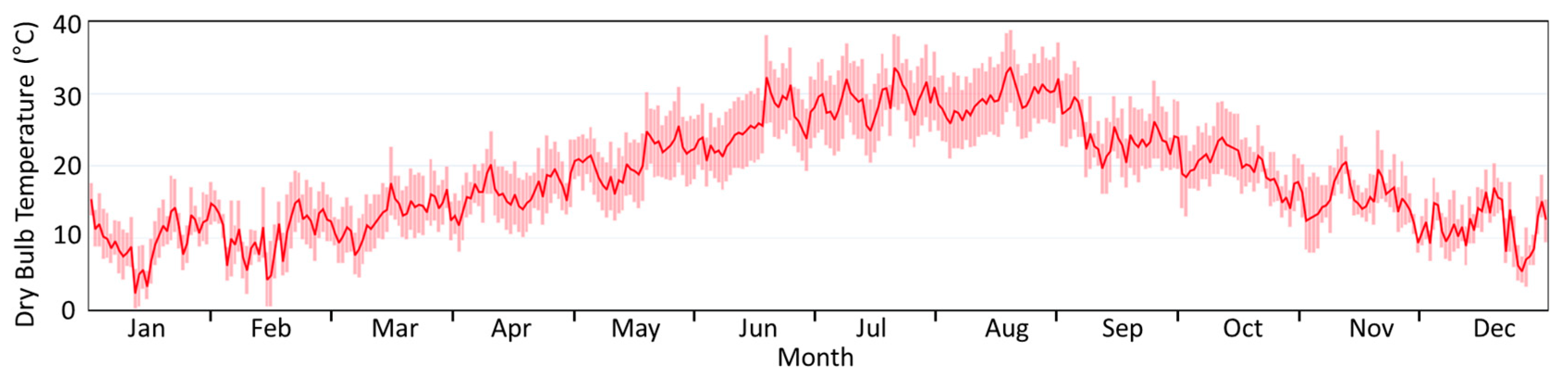
The Mediterranean climate of Athens includes prolonged hot and dry summers and mild, wet winters with moderate rainfall. July and August are the driest months with the highest outdoor dry bulb temperatures, and diurnal variations in outdoor temperatures are notable (Figure 1). The dominant southwest wind comes with higher wind speeds to Athens throughout the year (Figure 2). The heating degree days (HDD) and cooling degree days (CDD) for the current climate of Athens show that the buildings in Athens need both heating and cooling for comfort (Figure 2).

Figure 1.
The daily outdoor dry bulb temperature profiles of Athens.
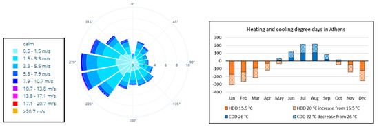
Figure 2.
A wind rose, heating degree day, and cooling degree day profiles of Athens.
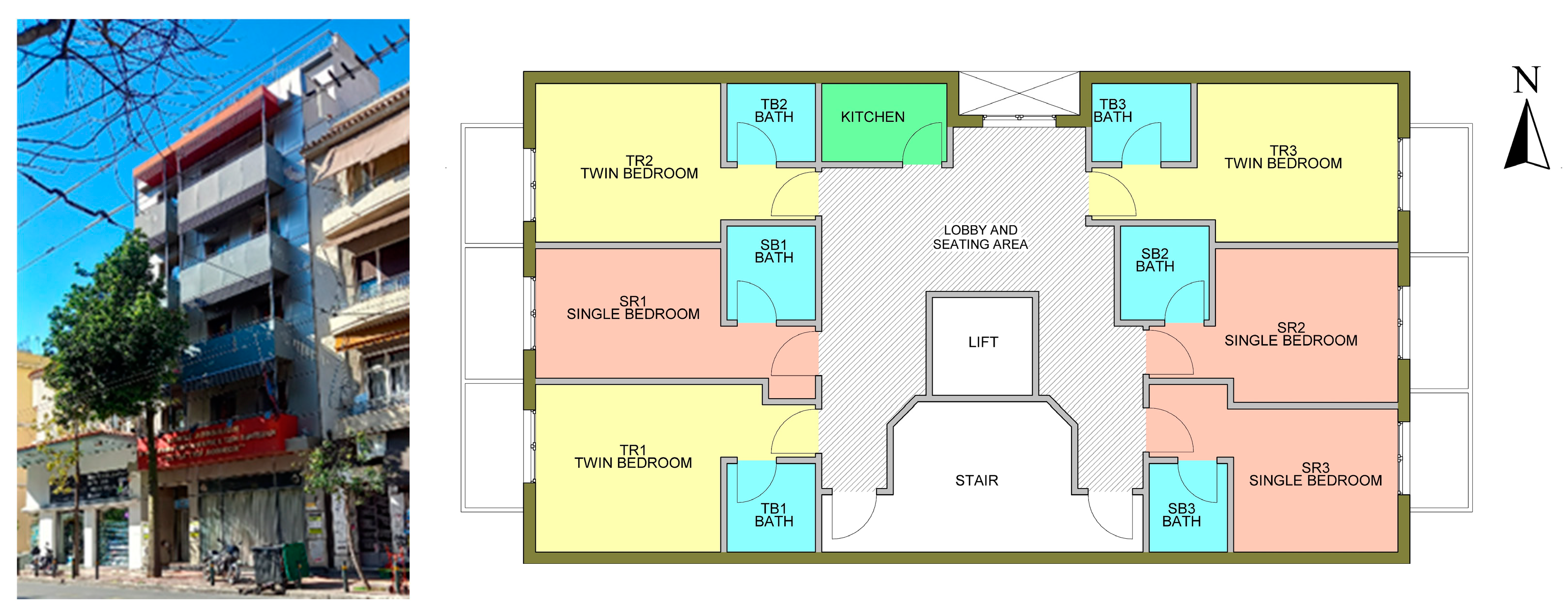
The case study building in Athens is located in a very dense urban texture within a well-defined urban canyon street. It is a five-story residential building, and it is highly representative of the low-rise multi-apartment buildings that were built during the 1930s. It was renovated in 2005 by adding rooftop insulation, installation of double-glazed aluminum windows to minimize thermal losses, and the replacement of outdated lighting with LED lamps. It is used as a hostel for homeless people and houses support staff, with a maximum capacity of 60 occupants. The total floor area is 1080 m2, and it has a ground floor, 5 stories, and a basement. It is located in Patission Street, which is a long street surrounded by similar height buildings starting from the center of Athens and extending to the north. The building is located about 3 km from the center of Athens (Omonia Square). A typical floor plan and an external view of the building are presented in Figure 3.
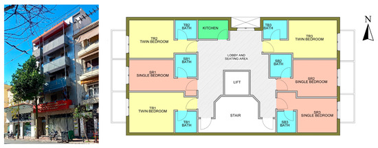
Figure 3.
External view and a typical floor plan of the case study building.
The heating and hot water system operates with natural gas. The apartments of the tenants are hotel-like rooms, including a bedroom and bathroom, with a TV and fan, and a heating and cooling thermostat. The thermal properties of the external envelope are presented in Table 1.

Table 1.
Thermal properties of the building envelope.
For this paper, two “intermediate levels”—Level 2 (above the ground floor) and level 4 (below the top floor)—were chosen. Each floor consists of six rooms—three single rooms (SR) and three twin rooms (TR). The single room is for one occupant, and the twin room is for two occupants. Each room has a balcony with one window/door on either the east or west side. The communal areas, which include the kitchen, lift, and stair core, are located in the middle of the building.
The building schedules (occupancy fraction, appliance and lighting usage, etc.) for a typical residential apartment, as recommended in the BSEN 16798 [26], were used in this study. Figure 4 presents the schedules used; 0 represents no activities, and 1 represents fully operated or active for one hour. According to the occupancy for weekdays and weekends, the heating hours, window opening hours, and mechanical ventilation time were applied. As the climate of Athens needs both active heating and cooling, either system were considered to operate if the indoor temperature was lower than 20 °C or higher than 26 °C [26]. The heating schedule was run from 05:00 to 23:00 except window opening hours; heating was turned off during the weekdays considering the lower occupancy. The cooling schedule was run according to occupant presence. Two different window-opening scenarios were considered in this work. One was that the window-opening time was proposed for two hours a day (morning and evening), and the other was to open the window during occupied hours if the indoor temperature was above 22 °C.
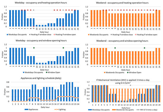
Figure 4.
Occupancy, appliance, lighting, heating, and ventilation schedules used in this study (the occupancy schedule is referred to BSEN 16798 [26]).
2.2. Methodology for Generating Urban Weather Files
The methodology for generating the urban weather files used in thermal simulations is presented in Figure 5. It accounts for the urban location of the building in calculations.
The Urban Weather Generator (UWG) was developed to generate urban canyon weather files using rural weather files as the input [27,28]. UWG is composed of four modules: a rural station model; a vertical diffusion model; an urban boundary layer model; and an urban canopy model, including a building energy model, which allows one to account for the impact of buildings on the urban air temperature. The modules are described in detail in the relevant publications by B. Bueno and J. Mao [27,28,29,30]. The MATLAB version of UWG V4.1 [31] was used for this analysis.
The urban weather file generated by UWG accounts for the heat fluxes from the roofs, walls, windows, and the road, as well as the anthropogenic heat fluxes due to exfiltration and waste heat from building HVAC systems and traffic. The input weather conditions were given by a “rural” weather file—generally the airport weather file—in the EnergyPlus format (.epw). In this study, two rural weather files (current and future) from Meteonorm were used [14] as the starting point. The future weather was considered for the RCP8.5 scenario, which is the worst case, high-emissions scenario for the year 2050 caused by “business as usual” without efforts to cut greenhouse gas emissions [32]. These weather files were used as the input to UWG calculations to generate future urban weather files that capture the local UHI intensity of the urban areas where the buildings are located.
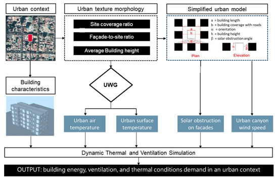
Figure 5.
The urban considerations in the building simulation (adapted from [33]).
Figure 5.
The urban considerations in the building simulation (adapted from [33]).

UWG generates urban weather files with morphed air temperature and relative humidity values based on the hourly UHI intensity of the urban area, keeping the other variables to the same value as in the input weather file. The urban area in UWG is described through a set of parameters that are representative of key urban fabric characteristics that affect UHI intensity, namely the following: urban morphology parameters, building typology mix, vegetation coverage, anthropogenic heat from traffic and albedo, and the thermal capacity and emissivity of urban materials. Among these, the most relevant were the urban morphology parameters [27,28,34,35]. Urban morphology is described using three parameters:
- Building density: the ratio of the building footprints area to the urban site area.
- Vertical-to-horizontal ratio: the ratio of the building facades area to the urban site area.
- Average building height: the average height of building normalized by the building footprint.
These were used to calculate the average width and height of the urban canyon for the computation of the external surface temperatures of walls, roads, and roofs based on the incoming, absorbed, and reflected radiation by urban surfaces.
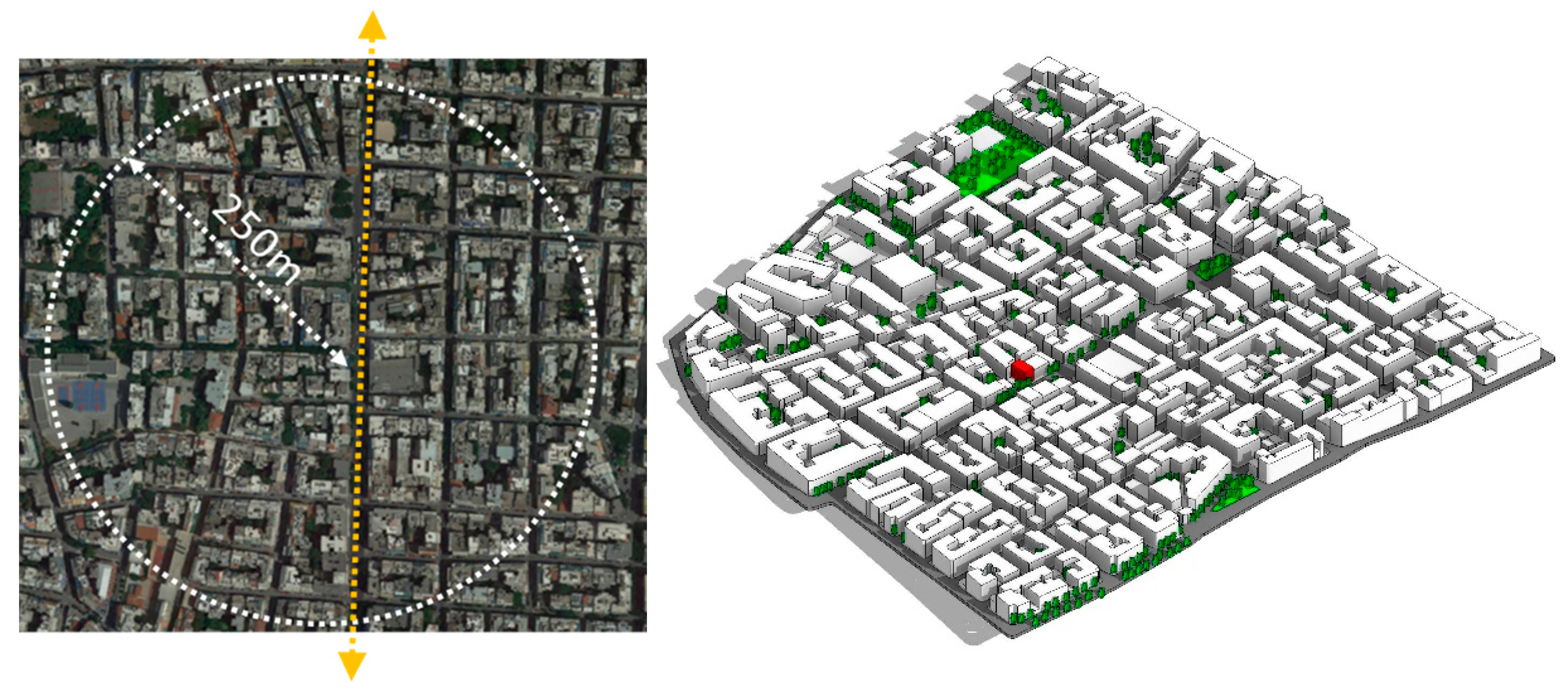
Autodesk Revit was used to generate the required building information for the UWG based on the urban area around the case study building, as shown in Figure 6 (left). Based on this area in Athens, a 3D model was created over an area of about 250 m in length, as suggested for local urban climate studies [36,37]. The case study building is located on the road (the yellow arrow shown in Figure 6), where the urban canyon wind was to be calculated. The topography of the site was modeled according to its location above sea level, where the south is lower than the north. The buildings were represented in the Revit massing models that allow for calculating the façade and floor areas of the site and average building height for the UWG program. The building types were defined for each 3D model that allows calculating the energy consumption for residential, primary, and secondary schools; retail shops; hotels; restaurants; supermarkets, etc. The building density, the urban buildings’ vertical-to-horizontal ratio, and the green area coverage were then calculated through the Revit area scheme. Evergreen trees were considered for the vegetation growing seasons. The massing models of urban buildings for the selected site are shown in Figure 6. After the UWG’s.xlsm files and other source files were co-simulated using MATLAB, two urban weather files for current and future scenarios were obtained. Table 2 presents the input values calculated.
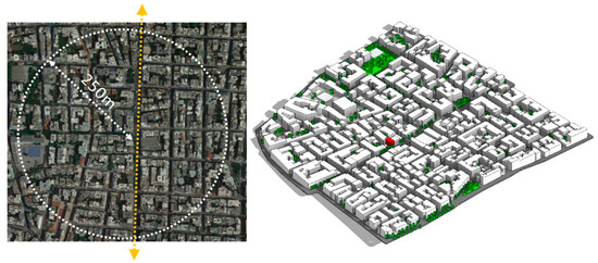
Figure 6.
The site plan and 3D massing model of the case study location (the case study building is shown in red colour).
Table 2.
The input data used in the UWG’s.xlsm file.
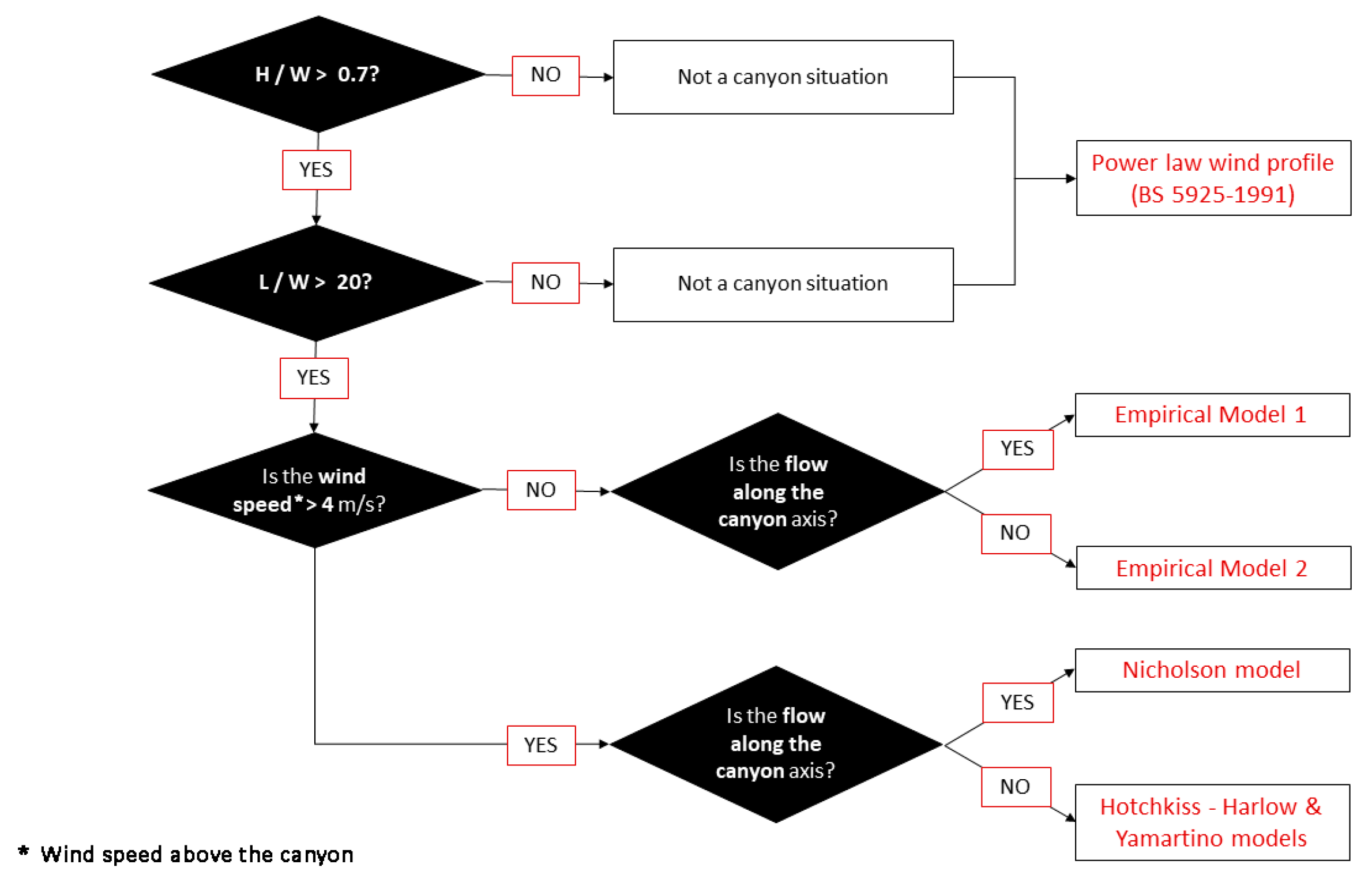
The hourly wind speed attenuation in the canyon was calculated using the algorithms of [38], as presented by [33]. These calculations are based on empirical models based on extensive measurements carried out and presented in [33] within urban canyons in Athens. Figure 7 presents the different urban situations, depending on the geometry and orientation of the canyon, and the wind speed and direction at the meteorological station. For this paper, the terrain type with a roughness of 5.0 was assumed, which is a typical value for a dense urban area. The average urban height, building density, and vertical-to-horizontal building area ratio were calculated using the same data generated for the UWG program. The length-to-width ratio of the road was more than 20; hence, the canyon height-to-width ratio was checked, and it was identified that the case study building was exposed to the urban canyon wind. The case study building had five stories; the urban canyon wind was, therefore, required to be calculated from its relative building height above the ground level. It was considered 7 m above street level for Level 2 and 15 m height for Level 4. Hourly wind speed values of canyon wind were calculated for the undisturbed wind, and wind direction values were found in the rural weather files. The urban canyon wind speed values were then replaced with the urban weather files generated from the UWG program.

Figure 7.
Algorithm for the calculation of wind speed in urban canyons [38].
Incorporating urban characteristics within future weather files may not be as straightforward as in the case of current weather files. This is because the impact of climate change may not be linear in cities and will depend on its building density, morphology, and materials. However, the approach currently adopted in creating urban future climate files for simulation is to change future weather files using urban morphing software 2.0 to incorporate urban perturbations. This was adopted in this paper following previous work [39] and as practiced by other researchers [40].
Finally, the overshadowing impact was taken into account by incorporating the surrounding buildings in the Dynamic Thermal Model (DTM) used for the hourly simulations. The DTM tool used was Energy Plus, using the DesignBuilder interface [41].
2.3. Development of Climate Correlation Models
In many climates, heating and cooling are not required throughout the year. In the case of the building in Athens, the heating demand is very low or zero for the months of March to November. Cooling demand is low for the months of November to May. Therefore, there are months in the year (November and March/April/May) when, with informed operation by the occupants, the building could be operated in a free-floating mode (without the need for mechanical-assisted heating or cooling). For this to be successful, occupants need to know what to do during the day and night when it comes to using the windows to provide ventilation and cooling and using the shading to reduce/increase solar gains. The correlation model developed and presented in this paper facilitates informed operation by the occupants, which will provide acceptable internal environmental conditions.
Within the PRELUDE H2020 project [42], a climate correlation model was developed to help occupants of low-technology buildings (i.e., no sensors and actuators) to obtain information on how to operate ventilation openings and shading devices to achieve the best internal environmental conditions in their space. The development of the climate correlation model was presented at the AIVC Conference in 2022 [43], and a more detailed report can be found in [44]. In summary, for each building in which the model would be applied, a dynamic thermal (DTM) and daylighting simulation model needs to be developed, where the simulations are run for the whole year using appropriate weather files for the location and linear correlations are developed between the external and internal conditions. Then, using the equations of the linear correlations, a prediction can be made for internal conditions in the space given a forecast of the external conditions for the days of interest. Considering the variability and uncertainty of weather forecasts, predictions should be made for one or two days ahead. Using the predictions, suggestions to the occupants can be made on how to operate their windows and shading devices so that they achieve the best environment in terms of thermal comfort, indoor air quality, and daylighting.
The relatively simple linear correlation was used because the method should be able to be executed by working consulting engineers and building managers who might not be familiar with the use of more sophisticated data analysis techniques that could have been used, such as, for example, machine learning, a subset of artificial intelligence that has been used extensively in building data and energy analytics. The presented method requires only an engineer/architect familiar with DTM and Excel spreadsheets.
To derive climate correlations for the building, a specific DTM model was developed using its geometrical, construction, and operational characteristics, as presented in Section 2.1. The model requires correlation equations to predict both (a) internal operative temperatures from external air temperatures and (b) air flow rates from either the wind speed or temperature gradient between the inside and outside. Internal contaminant concentrations can then be calculated based on the air flow rate and using single-zone mass balance equations if the contaminant generation rate is known. Hourly simulations for one year were carried out for the building and its weather under different operational (window opening) scenarios. Correlations were derived for each scenario with the equations to be used for the Excel climate correlation model, as shown in Table 3. For the intervention tests, Scenario 3 was used because it was a relatively warm period.
Table 3.
Correlation equations for thermal comfort and ventilation.
2.4. Tests of the Climate Correlation Model
The climate correlation equations were implemented in an Excel spreadsheet to predict the internal temperature and CO2 as an indicator of the IAQ in the apartment. CO2 concentration was calculated within the spreadsheet from the occupancy data for emissions and predicted air flow rates using mass balance equations.
The test in the Athens building was carried out from 16 to 18 April 2024 during a relatively mild period when the building was operating in a free-floating mode. Before the intervention, we had discussions with the occupants on the purpose of this study and their consent was obtained. They were interested to see the results on how they could improve the conditions in their space and were keen to implement them. The results were subsequently presented to them and the manager of the building. They commented that the instructions were easy to follow and did not report any issues while operating the openings and shading.
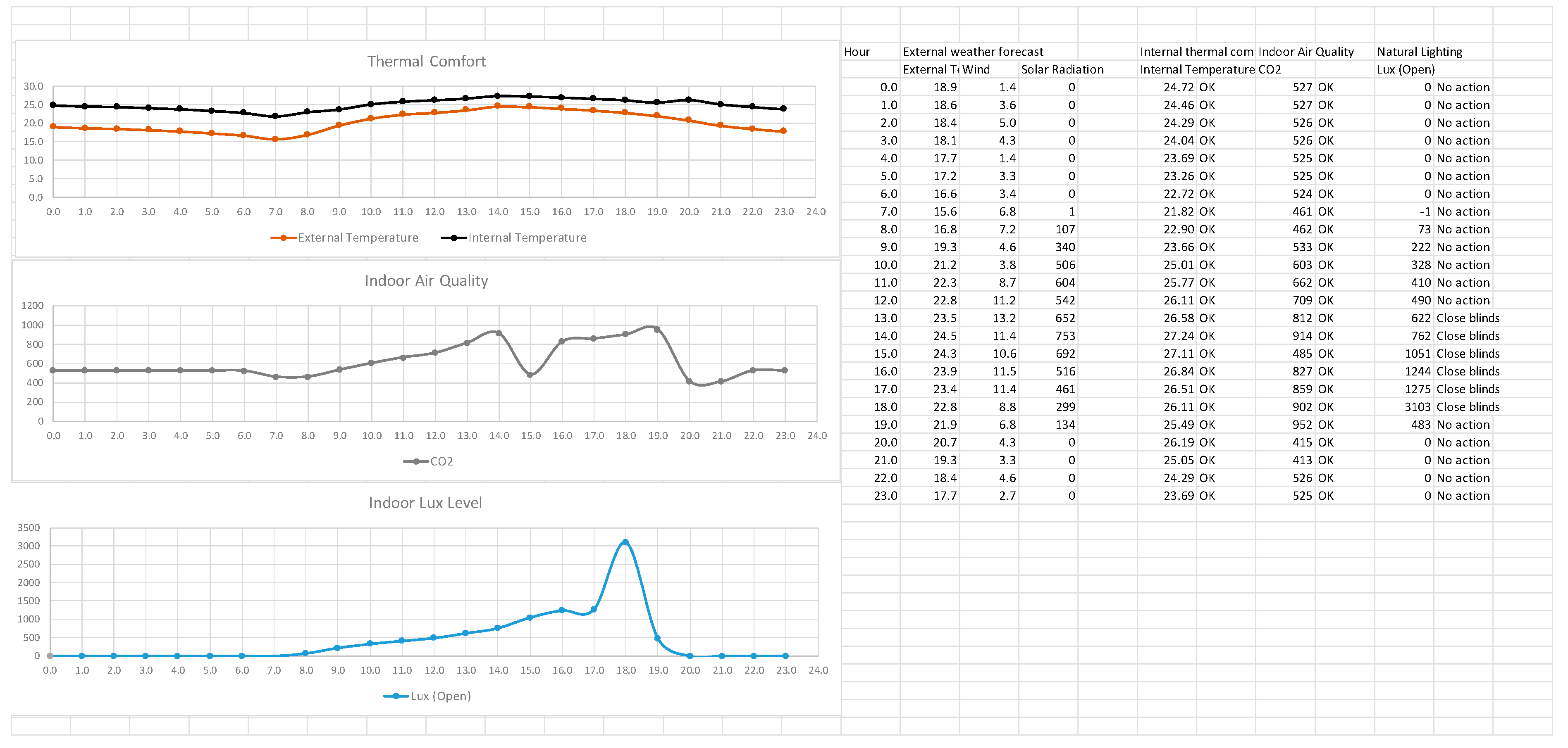
The day before the intervention (late in the evening), hourly forecast data were obtained using Open Meteo [45]. These included forecast hourly data for external temperature, wind speed, and global solar radiation, and they were input into the Excel tool. The Excel tool was run, and the optimum operation for windows and blinds was derived and sent to the building occupants via email. A screenshot of the simulation results is shown in Figure 8. This shows graphically the achievable air temperature, CO2, and natural lighting levels in the space according to Scenario 3 for window opening, which is two hours during the day (one in the morning and one in the afternoon) and during the night from 20:00 until 8:00. It indicates that thermal comfort and IAQ (using CO2 as the indicator) were satisfactory. It also shows how to use the shading (blinds closed between 13:00 and 18:00) to avoid high natural lighting levels, which can cause discomfort.
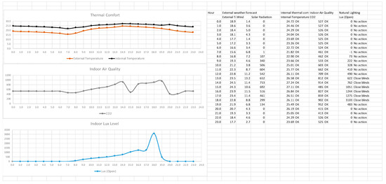
Figure 8.
A screenshot of the Excel tool predictions for 17 April 2024 in Athens.
The recommended actions sent to the occupants by email were as follows:
- Tuesday, 16 April and Wednesday, 17 April
- Close the window at 8 in the morning
- Open the window at 3 for one hour
- Open the window at 8 pm and leave it open during the night (and then close it at 8 in the morning).
- The window does not need to be completely open, just ajar, for example, 10 cm of opening (whatever is convenient—it does not matter how much it is open as long as it is open).
- If it is too cold at night, then they should close it and just tell us.
- Curtains should be closed between 3 p.m. and 6 p.m.
The occupants implemented the instructions very well, although they reported some variations as follows: They started the test on the morning of 16 April at 8 am when they opened the window for 30 min, and then they kept it closed as per instructions. They forgot to open the window at 15:00, but they did it the following day. The occupants reported that the instructions were clear and were able to follow them; they did not report any issues on external noise because of the open windows as their space opens to the back of the building away from the main road.
3. Results and Discussion
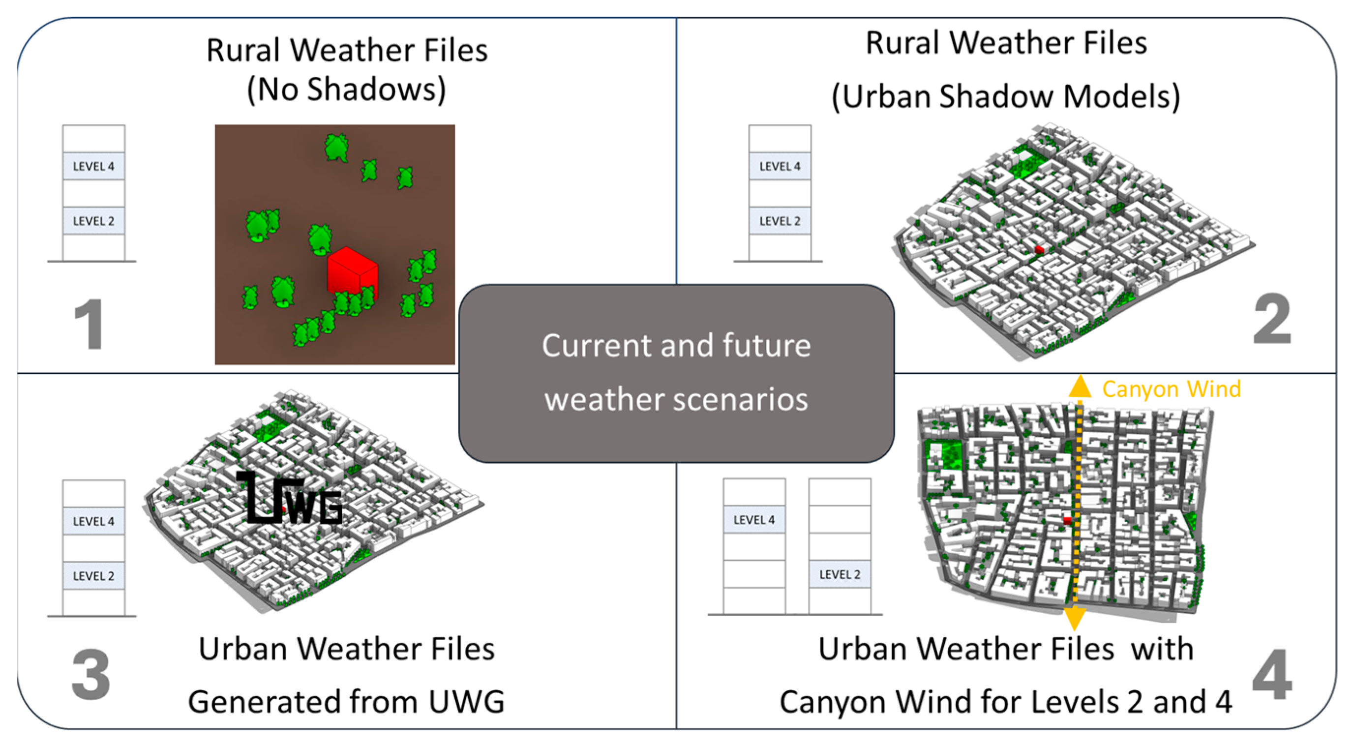
DTM simulations were carried out as described in Section 2.2. Data obtained from the building were used to define inputs for the EnergyPlus model, such as construction, schedules, and internal heat gains, which were supplemented by values from BSEN 16798-1 [26] when data were not available, as presented in Section 2.1. Figure 9 shows the four simulations performed. The first set of simulations were carried out using rural weather files with no overshadowing. The second set also used rural weather files with adjacent buildings in place to include overshadowing. The third set of simulations used urban weather files, as morphed using the Urban Weather Generator, including overshadowing. Finally, the fourth set of simulations used the urban weather files with wind speed corrections for the urban canyon and including overshadowing. The four sets of simulations were performed using current and future weather files, and the results were extracted for two levels in the building: Level 2 representing the lower floor, and Level 4 representing the higher floor.
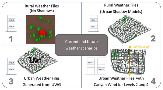
Figure 9.
The tested cases for current and future weather scenarios.
3.1. Comparison of Weather Files
The differences between the various weather files are compared in Figure 10. The comparison of the urban weather files with typical weather files showed, as expected, higher temperatures in the urban environment. This is well documented in the literature and has been reported by many studies and review papers (e.g., [46,47]). The results also show that the air temperature increases in future weather conditions, but the annual mean temperatures were lower than 21 °C in all scenarios. However, when the temperature values were assessed for the summer period only, a significant temperature increment could be observed in future weather conditions, reaching its summer average temperature above 31 °C, which will indicate that mechanically assisted cooling might be required during these months for internal thermal comfort. The analysis of wind speeds shows that it reduces significantly within the urban canyon. The average urban canyon wind speed, generated for Level 4, which is located 15 m above the ground level, was as low as 1.5 m/s and mostly still throughout the year. That implies decreasing natural ventilation efficacy for cooling in this location, which can only be predicted if the urban canyon modification is included in the weather files. It also changes the infiltration rate, which would affect heating and cooling demand.
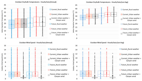
Figure 10.
Comparison of the outdoor dry bulb temperature and wind speed in different weather files.
3.2. Annual Energy Demand
The annual heating and cooling demand for the current and future weather conditions are presented in Figure 11 and Table 4 for the lower floor (L2) and higher floor (L4) of the building, as well as the roof (penthouse). For the roof-level rooms, the weather files were created by calculating the urban canyon wind at 18 m above street level.
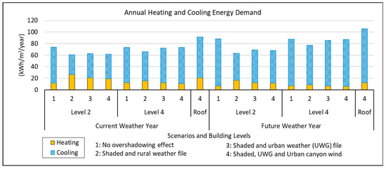
Figure 11.
The annual heating and cooling demand of Level 2, Level 4, and the roof.
Table 4.
The heating, cooling, and total energy demand for the various weather scenarios.
The results of the annual energy demand indicate, as expected, that future weather will demand higher cooling and lower heating because of an increase in external temperature. It also shows that there is a variation of energy demand on the vertical location of the space simulated. A higher floor would demand more cooling and less heating compared to a lower floor due to the lower wind speeds near the ground reducing infiltration and ventilation losses. The highest total energy demand would be for higher floors in the future. The results indicate higher heating and cooling demand because there were no overshadow effects, from the surrounding building and wind speeds were higher.
Table 4 shows the numerical results of the simulations. The change ratio is the ratio of the energy demand over the baseline weather file, which was not adapted (current weather). We can see that the heating demand was reduced at all levels by more than 50% for future urban weather, and the cooling increased much steeper for the penthouse; meanwhile, the overall energy demand will be 13% more for lower floors, 32% more for intermediate floors, and 75% for high floors.
These predictions, although they are indicative as they apply on scenarios about the future climate, using different scenarios or even methods to generate future weather data might give different absolute values [48], but the trend will remain similar.
3.3. Monthly Energy Demand
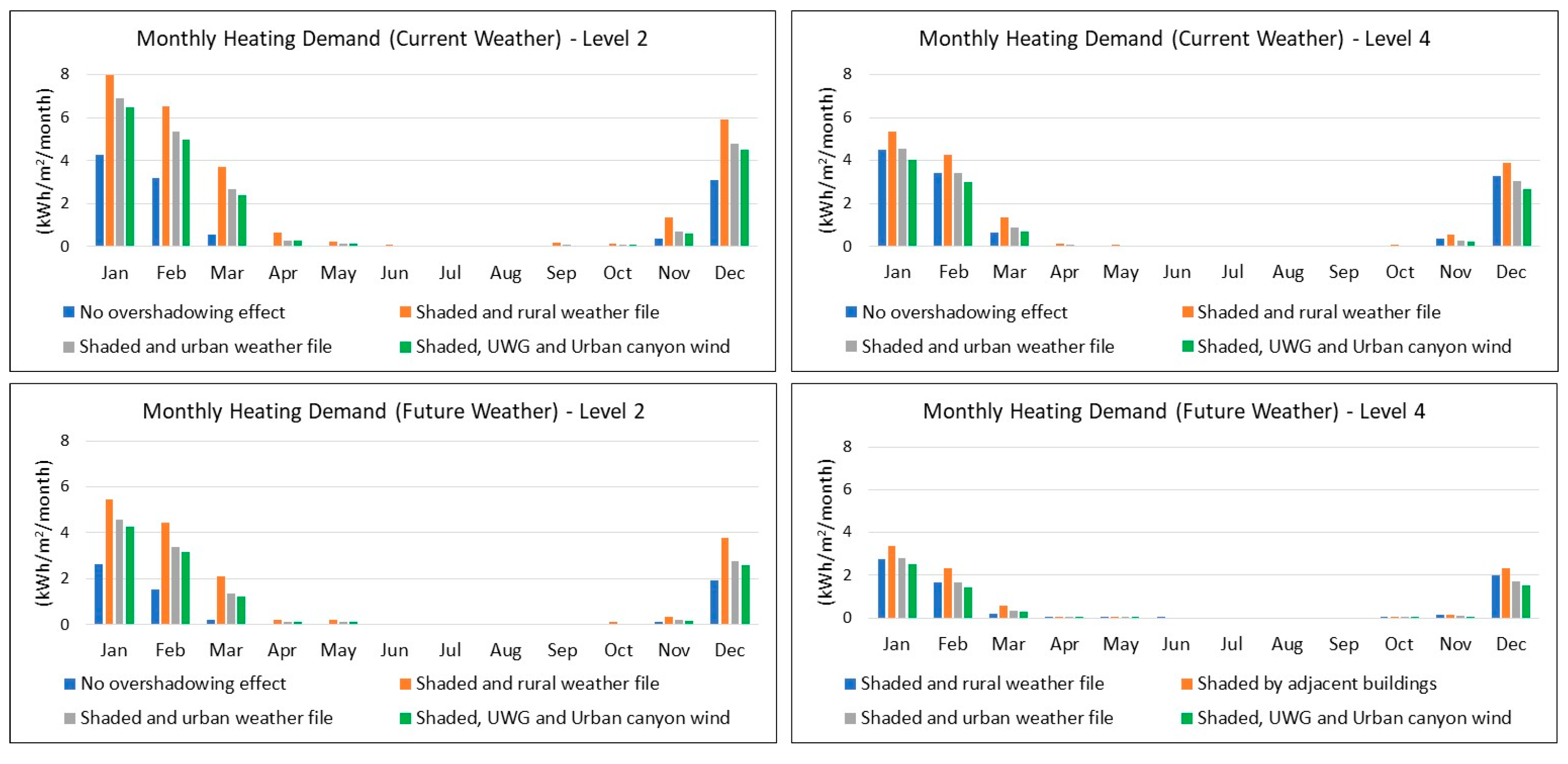
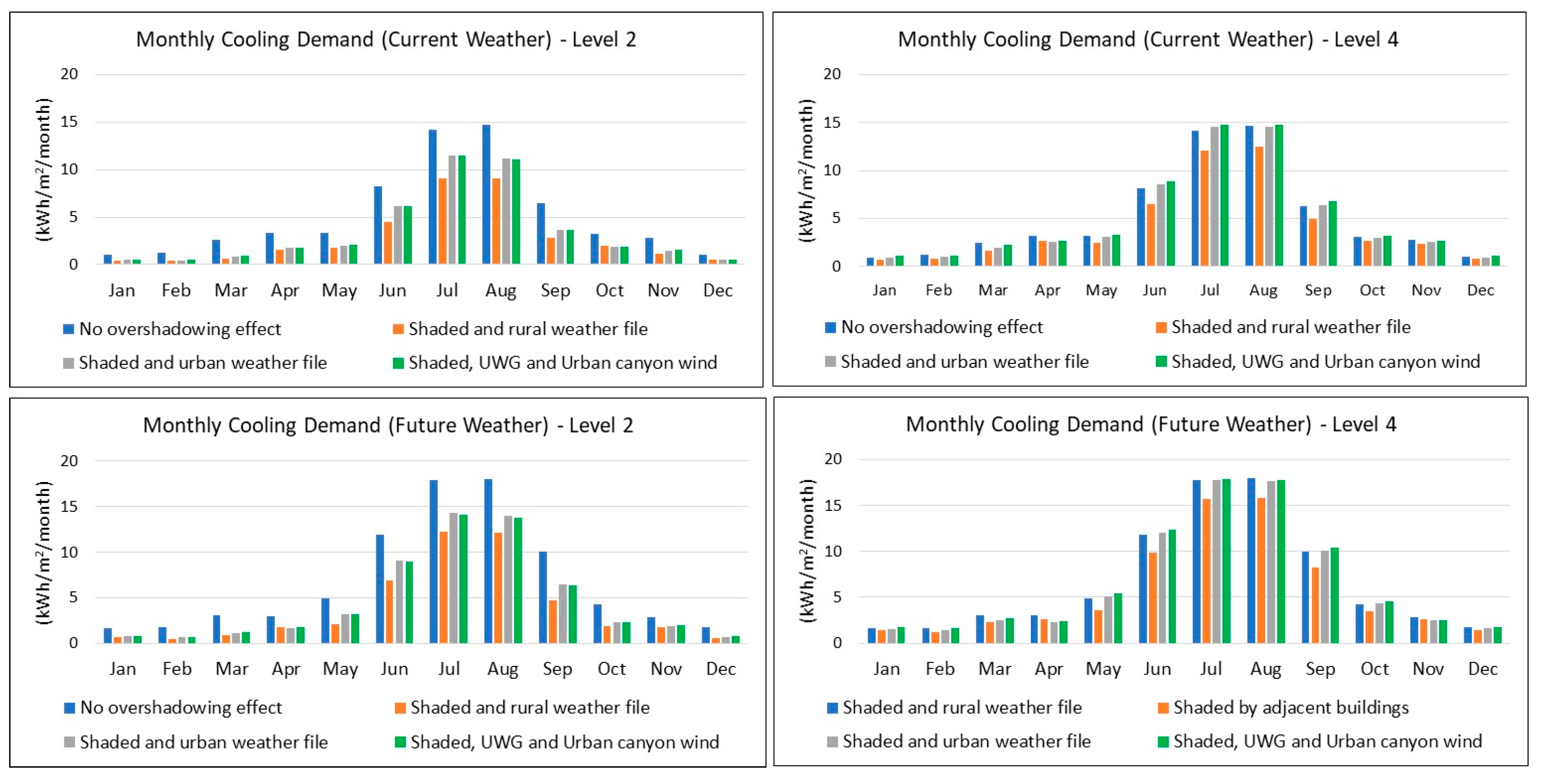
The impacts of weather and microclimatic conditions on monthly heating and cooling demand are presented in Figure 12 and Figure 13, where the difference between rural and urban weather files, overshadowing, and urban canyon wind effects are considered. Results using future weather files are also presented.
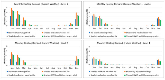
Figure 12.
The monthly heating demand of the Level 2 and Level 4 rooms.
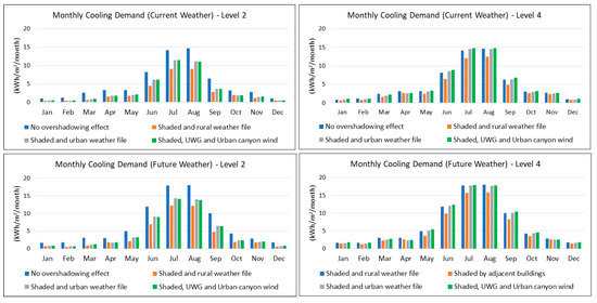
Figure 13.
The monthly cooling demand of the Level 2 and Level 4 rooms.
Figure 12 shows that heating demand was mainly from December to March due to the cold season in Athens. The heating demand of the building placed in the open terrain without adjacent buildings was less than the urban building because of the useful solar gains in a climate with relatively high solar radiation, even during the winter months. Therefore, simulating overshadowing is important as it would affect (increase) the heating demand significantly in all cases. As expected, using urban temperatures and future weather would reduce the heating demand because of the increase in outdoor air temperatures. Due to the effect of the urban canyon wind, the heating demand could be reduced because infiltration will be lower, reducing the impact of external cold air. At a building level, the heating demand of Level 2 is higher than Level 4 because of the overshadowing effect affecting lower floors more. Overshadowing seems to have a higher impact than infiltration on lower floors, which would have reduced heating demand because of lower wind speeds near the ground.
Figure 13 shows that cooling demand was mainly during the summer months of June to September. Contrary to the heating demand, the cooling demand of a building in the open terrain was higher than the urban building due to solar gains; therefore, simulating overshadowing was also important for a more accurate prediction of cooling demand. As expected, using urban temperatures and future weather would increase the cooling demand. Urban canyon wind had a very small impact on the cooling demand; one would have expected this because the infiltration is reduced because of lower wind speeds, and cooling demand would have reduced during the day and increased during the night. It seems that the overall effect saw a slight increase in cooling demand. At a building level, the cooling demand of Level 2 is less than Level 4 because of the overshadowing effect from the surrounding buildings, which reduces the solar heat gain. At the same time, because of the urban canyon wind, the cooling demand is slightly higher for Level 4; as in the case of heating demand, infiltration will be higher on higher floors, which will increase the cooling demand during the day and possibly reduce it during the night. However, the balance with the overshadowing impact results in a very slight increase in cooling demand at Level 4 because of urban wind.
3.4. Results of Climate Correlation Intervention Study
As discussed in Section 3.3, for the case study building in Athens, the heating demand was very low or zero for the months of March to November (Figure 12), and the cooling demand was low for the months of November to May (Figure 13). Therefore, there were months in the year (November and March/April/May) when the building could be operated in a free-floating mode (without the need for mechanical-assisted heating or cooling). During these periods, results by the climate correlation model would be very useful to inform occupants on how to operate their building more efficiently to maintain thermal comfort and indoor air quality without using energy.
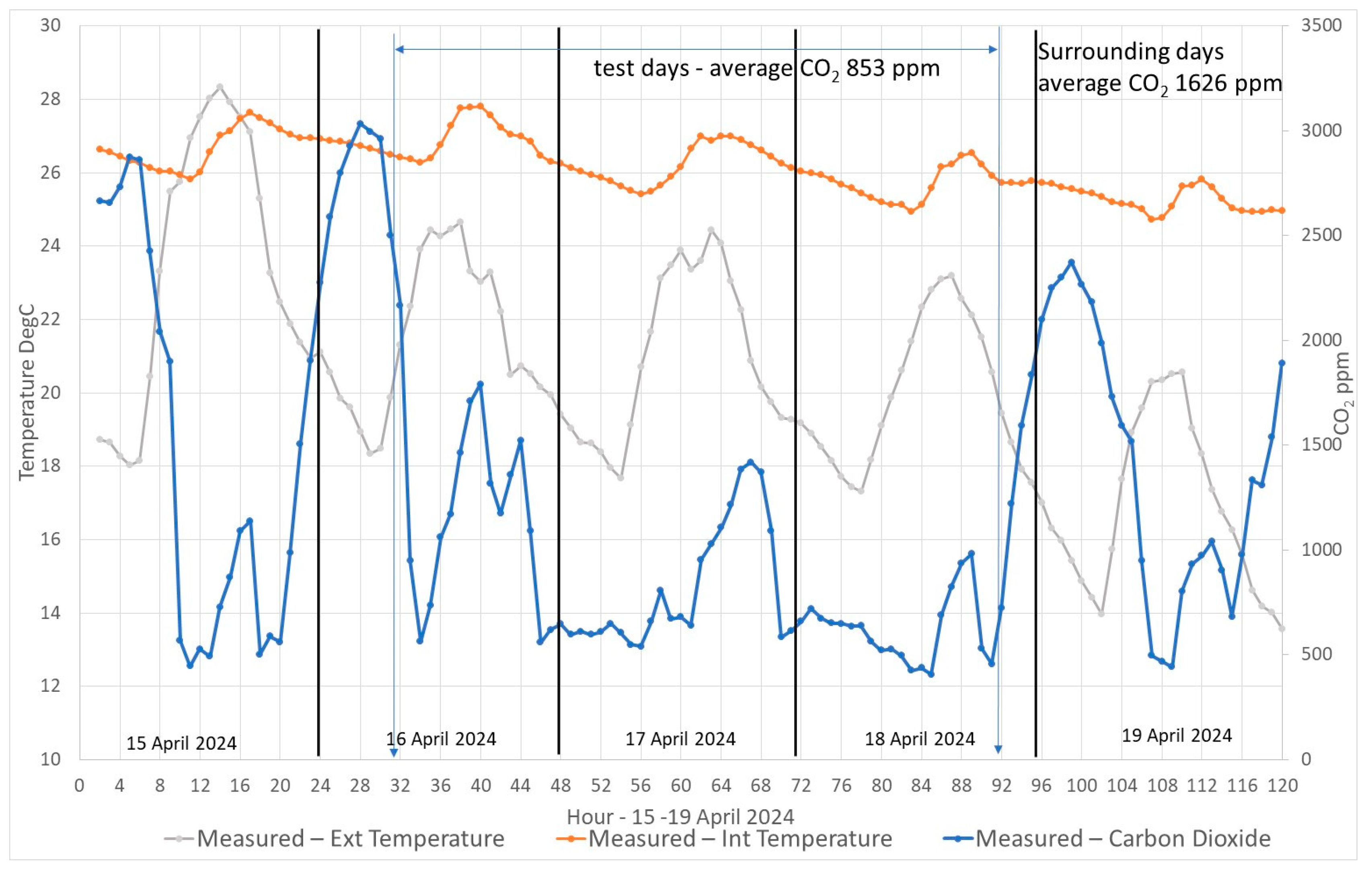
The predictions of the climate correlation model were compared with measured data in the building. A Hobo MX CO2 logger [49] was installed in one of the bedrooms for which the occupants were willing to take part in the study. The logger measured air temperature and CO2 in 30 min intervals. Figure 14 presents the measured data in the bedroom during the two days of the test and the surrounding days. It can be seen clearly that the CO2 level was much lower during the test days, indicating improved IAQ through ventilation. The average CO2 level was 853 ppm during the test days in comparison to 1626 ppm during the two surrounding days. The temperature trace also showed that internal thermal comfort was acceptable despite opening the window at night and the weather becoming a bit colder. The occupants seemed to stay in their room during the afternoon, and, in hindsight, opening the window in the afternoon for more than one hour should have been recommended. Nevertheless, the CO2 levels are acceptable, especially on the second afternoon when the window was opened for one hour as recommended (18 April).
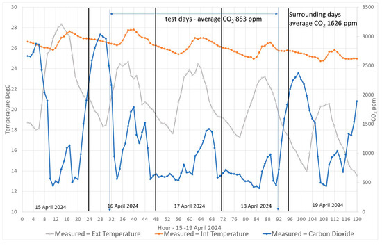
Figure 14.
Environmental conditions in the bedroom for the two days of the test and surrounding days.
The occupant’s behavior in opening windows has been identified in other recent studies [50], indicating that information about what to do during different weather conditions would affect the quality of internal comfort.
4. Conclusions
This paper has shown (using an operational residential case study building in Athens) that the urban environment has a significant impact on both the heating and cooling energy demand of a building. The impact depends on the urban density, urban textures, and exposure to the wind. Future climate change will also have an impact combined with the changes due to the urban microclimate. Six weather files were generated using UWG (changes in temperature) and urban canyon wind calculation. In addition, the overshadowing effects were simulated. The results of the simulation experiment showed the following:
- The heating demand could decrease in future, while the cooling demand could increase due to the increase in outdoor dry bulb temperature.
- Results vary with the height of the space, with higher floors demanding less energy for heating and higher energy for cooling, and this is mainly due to overshadowing, which changes solar gains.
- There are increased external temperatures due the UHI decrease heating energy demand and increased cooling energy demand when overshadowing is also considered.
- The urban canyon wind caused lower wind speed, which influences energy consumption (due to changes in infiltration rates). This is more pronounced for the heating demand.
- There are extensive periods in the year when both heating and cooling energy demand is very low; thus, the building could be used in a free floating (no cooling, heating, or mechanical ventilation) mode during these periods.
In order to ensure good internal environmental quality during the times that the building is operated in free-floating mode in low-technology buildings (which is the majority of older residential buildings), occupants need to know how to use windows and shade according to external prevailing conditions. A method is outlined on how this can be done and was applied in the case study building with encouraging measured results.
5. Limitations and Further Research
This paper focused on a specific case study building with certain thermal characteristics; other buildings with different patterns of use (affecting internal heat gains) and thermal characteristics (construction of external envelope) might respond differently, although we believe that the trend will be similar. This variation has not been addressed in this work, so applicability for other buildings is required for it to be investigated further.
Statistical tests to investigate quantitatively how much of the data variance can be explained with the proposed model have not been included in this paper. This needs to be addressed in future work of the model’s development together with its applicability for other building types and construction.
This work used typical weather files for the simulations. Variations of weather to include heatwaves have not been incorporated; this will primarily affect the internal conditions during free-floating use of the building and that, to a lesser extent, cooling loads depending on the frequency and length of heatwaves.
The occupant-facilitated operation, during periods when cooling or heating is not needed, was tested in the operational building for a period of two days. Further testing and feedback by the occupants will add to the validity and efficacy of the proposed actions. In addition, the impact of external conditions, such as the external noise and levels of external pollution, should be considered depending on the position of the space in the urban context.
Author Contributions
Conceptualization, M.K. and M.Z.; methodology, M.K., M.Z., P.G., T.P.T., I.C. and D.T.; software, M.Z. and T.P.T.; validation, M.Z., I.C. and D.T.; formal analysis, M.K.; P.G. and M.Z.; investigation, M.K., M.Z., P.G.; T.P.T., I.C. and D.T.; resources, M.K., M.Z., P.G., T.P.T., I.C. and D.T.; data curation, I.C. and D.T.; writing—original draft preparation, M.K. and P.G.; writing—review and editing, M.Z., P.G.; T.P.T., I.C. and D.T.; visualization, M.Z. and P.G.; supervision, M.K.; project administration, M.K.; funding acquisition, M.K., I.C. and D.T. All authors have read and agreed to the published version of the manuscript.
Funding
This research was funded by the European Union’s Horizon 2020 research and innovation program under Grant Agreement N° 958345 for the PRELUDE project (https://prelude-project.eu, accessed on 11 March 2025).
Data Availability Statement
The original contributions presented in this study are included in the article material. Further inquiries can be directed to the corresponding authors.
Acknowledgments
We gratefully acknowledge the collaboration of the occupants and managers of the case study building in Athens; this study would not have been possible without them. We are also grateful to the reviewers for pertinent comments which improved the paper.
Conflicts of Interest
Authors Ilia Christantoni and Dimitra Tsakanika were employed by DAEM SA, City of Athens IT Company. The remaining authors declare that the research was conducted in the absence of any commercial or financial relationships that could be construed as a potential conflict of interest.
References
- Heiselberg, P. (Ed.) EBC Annex 62 Ventilative Cooling: Project Summary Report; IEA EBC: Canberra, Australia, 2019; Available online: https://www.iea-ebc.org/Data/publications/EBC_SR_Annex62.pdf (accessed on 5 March 2025).
- Morales, R.D.; Audenaert, A.; Verbeke, S. Thermal comfort and indoor overheating risks of urban building stock—A review of modelling methods and future climate challenge. Build. Environ. 2024, 269, 112363. [Google Scholar] [CrossRef]
- Bueno, B.; Roth, M.; Norford, L.; Li, R. Computationally efficient prediction of canopy level urban air temperature at the neighbourhood scale. Urban. Clim. 2014, 9, 35–53. [Google Scholar] [CrossRef]
- Jusuf, S.K.; Wong, N.H. Development of Empirical Models For an Estate Level Air Temperature Prediction in Singapore, Berkeley, United States. In Proceedings of the 7th International Conference on Urban Climate, Yokohama, Japan, 29 June–3 July 2009. [Google Scholar]
- Kershaw, T.; Sanderson, M.; Coley, D.; Eames, M. Estimation of the urban heat island for UK climate change projections. Build. Serv. Eng. Res. Technol. 2010, 31, 251–263. [Google Scholar] [CrossRef]
- De Ridder, K.; Lauwaet, D.; Maiheu, B. UrbClim—A fast urban boundary layer climate model. Urban. Clim. 2015, 12, 21–48. [Google Scholar] [CrossRef]
- Mauree, D.; Coccolo, S.; Kaempf, J.; Scartezzini, J.-L. Multi-scale modelling to evaluate building energy consumption at the neighbourhood scale. PLoS ONE 2017, 12, e0183437. [Google Scholar] [CrossRef]
- Fahssis, K.; Dupont, G.; Leyronnas, P. UrbaWind, A Computational Fluid Dynamics Tool to Predict Wind Resource in Urban Area. 2010. Available online: https://www.scribd.com/document/151322723/UrbaWind-a-Computational-Fluid-Dynamics-tool-to-predict-wind-resource-in-urban-area (accessed on 5 March 2025).
- Bruse, M.; Fleer, H. Simulating surface–plant–air interactions inside urban environments with a three dimensional numerical model. Environ. Model. Softw. 1998, 13, 373–384. [Google Scholar] [CrossRef]
- Merlier, L.; Frayssinet, L.; Kuznik, F.; Rusaoue¨n, G.; Johannes, K.; Hubert, J.-L.; Milliez, M. Analysis of the (Urban) Microclimate Effects On the Building Energy Behaviour; IBPSA: Fairfax, VA, USA, 2017; pp. 1780–1787. [Google Scholar] [CrossRef]
- Jentsch, M.F.; James, P.A.B.; Bourikas, L.; Bahaj, A.S. Transforming existing weather data for worldwide locations to enable energy and building performance simulation under future climates. Renew. Energy 2013, 55, 514–524. [Google Scholar] [CrossRef]
- Moazami, A.; Carlucci, S.; Geving, S. Critical Analysis of Software Tools Aimed at Generating Future Weather Files with a view to their use in Building Performance Simulation. Energy Procedia 2017, 132, 640–645. [Google Scholar] [CrossRef]
- Jiang, A.; Liu, X.; Czarnecki, E.; Zhang, C. Hourly weather data projection due to climate change for impact assessment on building and infrastructure, Sustain. Cities Soc. 2019, 50, 101688. [Google Scholar] [CrossRef]
- Meteonorm Software. Available online: https://meteonorm.com/en/ (accessed on 5 March 2025).
- Lauwaet, D.; Hooyberghs, H.; Maiheu, B.; Lefebvre, W.; Driesen, G.; Van Looy, S.; De Ridder, K. Detailed Urban Heat Island Projections for Cities Worldwide: Dynamical Downscaling CMIP5 Global Climate Models. Climate 2015, 3, 391–415. [Google Scholar] [CrossRef]
- Machard, A.; Salvati, A.; Tootkaboni, M.P.; Gaur, A.; Zou, J.; Wang, L.L.; Baba, F.; Ge, H.; Bre, F.; Bozonnet, E.; et al. Typical and extreme weather datasets for studying the resilience of buildings to climate change and heatwaves. Sci. Data 2024, 11, 531. [Google Scholar] [CrossRef]
- Sulzer, M.; Christen, A.; Matzarakis, A. Predicting indoor air temperature and thermal comfort in occupational settings using weather forecasts, indoor sensors, and artificial neural networks. Build. Environ. 2023, 234, 110077. [Google Scholar] [CrossRef]
- Kalidindi, S.S.V.; Banaee, H.; Karlsson, H.; Loutfi, A. Indoor temperature prediction with context-aware models in residential buildings. Build. Environ. 2023, 244, 110772. [Google Scholar] [CrossRef]
- Schweizer, C.; Edwards, R.D.; Bayer-Oglesby, L.; Gauderman, W.J.; Ilacqua, V.; Jantunen, M.J.; Lai, H.K.; Nieuwenhuijsen, M.; Künzli, N. Indoor time–microenvironment–activity patterns in seven regions of Europe. J. Expo. Sci. Environ. Epidemiol. 2007, 17, 170–181. [Google Scholar] [CrossRef] [PubMed]
- Givoni, B. Passive and Low Energy Cooling of Buildings; Van Nostrand Reinhold: New York, NY, USA, 1994. [Google Scholar]
- Manzano-Agugliaro, F.; Montoya, F.G.; Sabio-Ortega, A.; García-Cruz, A. Review of bioclimatic architecture strategies for achieving thermal comfort. Renew. Sustain. Energy Rev. 2015, 49, 736–755. [Google Scholar] [CrossRef]
- Ozarisoy, B.; Altan, H. Systematic literature review of bioclimatic design elements: Theories, methodologies and cases in the South-eastern Mediterranean climate. Energy Build. 2021, 250, 111281. [Google Scholar] [CrossRef]
- Elaouzy, Y.; Fadar, A.E. Energy, economic and environmental benefits of integrating passive design strategies into buildings: A review. Renew. Sustain. Energy Rev. 2022, 167, 112828. [Google Scholar] [CrossRef]
- Kolokotroni, M.; May, Z.; Tun, T.P.; Christantoni, I.; Tsakanika, D. Urban context and climate change impact on the thermal performance and ventilation of residential buildings: A case-study in Athens. In Proceedings of the 43nd AIVC Conference: Ventilation, IEQ and Health in Sustainable Buildings, Copenhagen, Denmark, 4–5 October 2023. [Google Scholar]
- Kolokotroni, M.; May, Z.; Tun, T.P.; Christantoni, I.; Tsakanika, D.; Stawowczyk, D.; de Kerchove d’Exaerde, T. Intervention study of climate correlation model predictions for occupant control of indoor environment. In Proceedings of the 44nd AIVC Conference: Retrofitting the Building Stock: Challenges and Opportunities for Indoor Environmental Quality, Dublin, Ireland, 9–10 October 2024. [Google Scholar]
- BS EN 16798-1; Energy Performance of Buildings. Ventilation for Buildings. Indoor Environmental Input Parameters for Design and Assessment of Energy Performance of Buildings Addressing Indoor Air Quality, Thermal Environment, Lighting, and Acoustics. Module M1-6. BSI: London, UK, 2019.
- Bueno, B.; Norford, L.; Hidalgo, J.; Pigeon, G. The urban weather generator. J. Build. Perform. Simul. 2013, 6, 269–281. [Google Scholar] [CrossRef]
- Mao, J.; Yang, J.H.; Afshari, A.; Norford, L.K. Global sensitivity analysis of an urban microclimate system under uncertainty: Design and case study. Build. Environ. 2017, 124, 153–170. [Google Scholar] [CrossRef]
- Bueno, B.; Norford, L.; Pigeon, G.; Britter, R. Combining a detailed building energy model with a physically-based urban canopy model. Bound.-Lay. Meteorol. 2011, 140, 471–489. [Google Scholar] [CrossRef]
- Bueno, B.; Hidalgo, J.; Pigeon, G.; Norford, L.; Masson, V. Calculation of air temperatures above the urban canopy layer from measurements at a rural operational weather station. J. Appl. Meteorol. Climatol. 2013, 52, 472–483. [Google Scholar] [CrossRef]
- Mao, J. UWG V4 MATLAB Code. 2018. Available online: https://github.com/hansukyang/UWG_Matlab (accessed on 5 March 2025).
- IPCC. Synthesis Report. In Contribution of Working Groups I, II and III to the Fifth Assessment Report of the Intergovernmental Panel on Climate Change; IPCC: Geneva, Switzerland, 2014. [Google Scholar]
- Salvati, A.; Palme, M.; Chiesa, G.; Kolokotroni, M. Built form, urban climate and building energy modelling: Case-studies in rome and Antofagasta. J. Build. Perform. Simul. 2020, 13, 209–225. [Google Scholar] [CrossRef]
- Nakano, A. Urban Weather Generator User Interface Development: Towards a Usable Tool for Integrating Urban Heat Island Effect Within Design Process. 2015, pp. 1–141. Available online: https://dspace.mit.edu/handle/1721.1/99251 (accessed on 5 March 2025).
- Salvati, A.; Kolokotroni, M. Microclimate Data For Building Energy Modelling: Study On ENVI-Met Forcing Data. In Proceedings of the 16th IBPSA Conference, Rome, Italy, 2–4 September 2019; Corrado, V., Gasparella, A., Eds.; pp. 3361–3368. [Google Scholar]
- Salvati, A.; Coch, H.; Cecere, C. Urban Heat Island Prediction in the Mediterranean Context: An Evaluation of the Urban Weather Generator Model. ACE Archit. City Environ. Arquit. Ciudad. Entorno 2016, 11, 135–156. [Google Scholar] [CrossRef]
- Stewart, I.D.; Oke, T.R. Local Climate Zones for Urban Temperature Studies. Bull. Am. Meteorol. Soc. 2012, 93, 1879–1900. [Google Scholar] [CrossRef]
- Ghiaus, C.; Allard, F.; Santamouris, M.; Georgakis, C.; Roulet, C.A.; Germano, M.; Tillenkamp, F.; Heijmans, N.; Nicol, J.; Maldonado, E.; et al. Natural Ventilation of Urban Buildings-Summary of URBVENT Project. In Proceedings of the International Conference “Passive and Low Energy Cooling for the Built Environment”, Santorini, Greece, 19–21 May 2005; pp. 29–33. [Google Scholar]
- Salvati, A.; Kolokotroni, M. Urban microclimate and climate change impact on the thermal performance and ventilation of multi-family residential buildings. Energy Build. 2023, 1132, 29424. [Google Scholar] [CrossRef]
- Hostein, M.; Musy, M.; Moujalled, B.; El Mankibi, M. Generating meteorological files of future climates with heatwaves in urban context to evaluate building overheating: An energy-efficient dwelling case study. Build. Environ. 2024, 263, 111874. [Google Scholar] [CrossRef]
- Design Builder Software. Available online: https://designbuilder.co.uk/ (accessed on 5 March 2025).
- PRELUDE: Prescient Building Operation Utilizing Real-Time Data for Energy Dynamic Optimization. 2025. Available online: https://prelude-project.eu/ (accessed on 5 March 2025).
- Zune, M.; Kolokotroni, M. Climate correlation model to forecast thermal comfort and IAQ in naturally ventilated residential buildings. In Proceedings of the 42nd AIVC Conference: Ventilation Challenges in a Changing World, Rotterdam, The Netherlands, 5–6 October 2022. [Google Scholar]
- Zune, M.; Kolokotroni, M. D3.4: Indoor-Outdoor Correlation Module. PRELUDE Project WP3: Interoperable Dynamic Module Integration in Multisimulation Dataspace. 2022. Available online: https://prelude-project.eu/results/deliverables/ (accessed on 5 March 2025).
- Open Meteo, Free Weather API. Available online: https://open-meteo.com (accessed on 5 March 2025).
- Kim, S.W.; Brown, R.D. Urban heat island (UHI) intensity and magnitude estimations: A systematic literature review. Sci. Total Environ. 2021, 779, 146389. [Google Scholar] [CrossRef]
- Rajagopal, P.; Priya, R.S.; Senthil, R. A review of recent developments in the impact of environmental measures on urban heat island. Sustain. Cities Soc. 2023, 88, 104279. [Google Scholar] [CrossRef]
- Duan, Z.; de Wilde, P.; Attia, S.; Zuo, J. Challenges in predicting the impact of climate change on thermal building performance through simulation: A systematic review. Appl. Energy 2025, 382, 125331. [Google Scholar] [CrossRef]
- HOBO MX CO2 Logger. Available online: https://www.tempcon.co.uk/hobo-mx1102-bluetooth-co2-temp-rh-data-logger (accessed on 5 March 2025).
- Jara-Baeza, F.; Rajagopalan, P.; Andamon, M.M. The impact of occupants’ window opening behaviour during summertime overheating in high-rise social housing. Energy Build. 2025, 330, 115331. [Google Scholar] [CrossRef]


Disclaimer/Publisher’s Note: The statements, opinions and data contained in all publications are solely those of the individual author(s) and contributor(s) and not of MDPI and/or the editor(s). MDPI and/or the editor(s) disclaim responsibility for any injury to people or property resulting from any ideas, methods, instructions or products referred to in the content. |
© 2025 by the authors. Licensee MDPI, Basel, Switzerland. This article is an open access article distributed under the terms and conditions of the Creative Commons Attribution (CC BY) license (https://creativecommons.org/licenses/by/4.0/).