
Optimization of Rotary Friction Welding Parameters Through AI-Augmented Digital Twin Systems


Abstract
1. Introduction
2. Materials and Methods
2.1. DT Based on MES
2.2. DT Based on ANN
2.3. GA-Based Optimization
3. Results
3.1. FEM Results
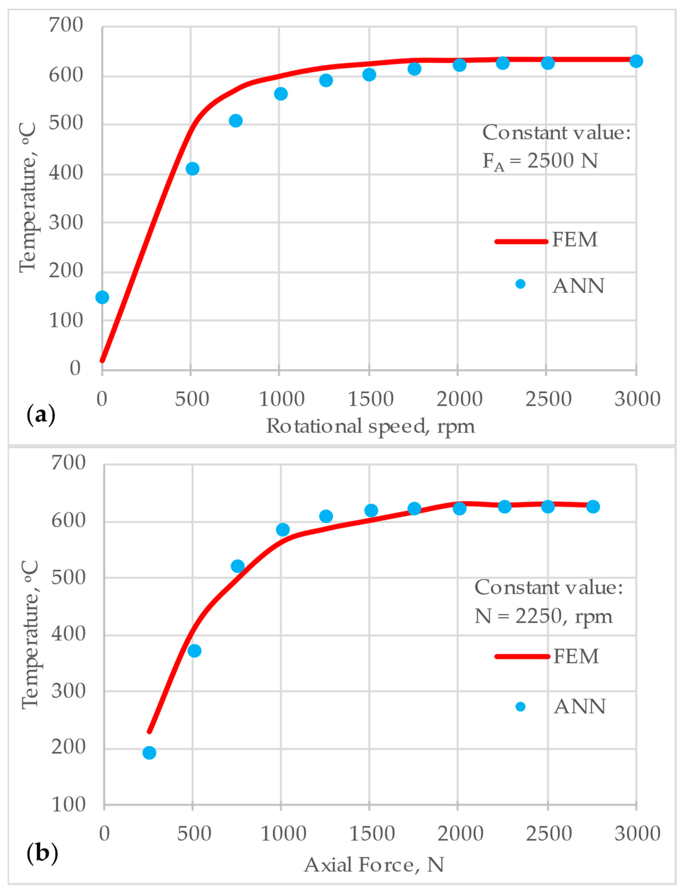
3.2. ANN Results
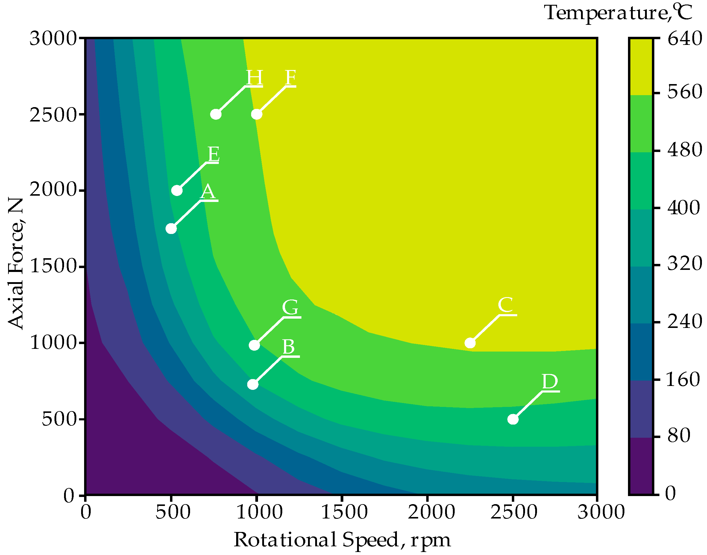
3.3. GA Result
4. Discussion
5. Conclusions
5.1. ANN Model Performance
5.2. Optimization via GAs
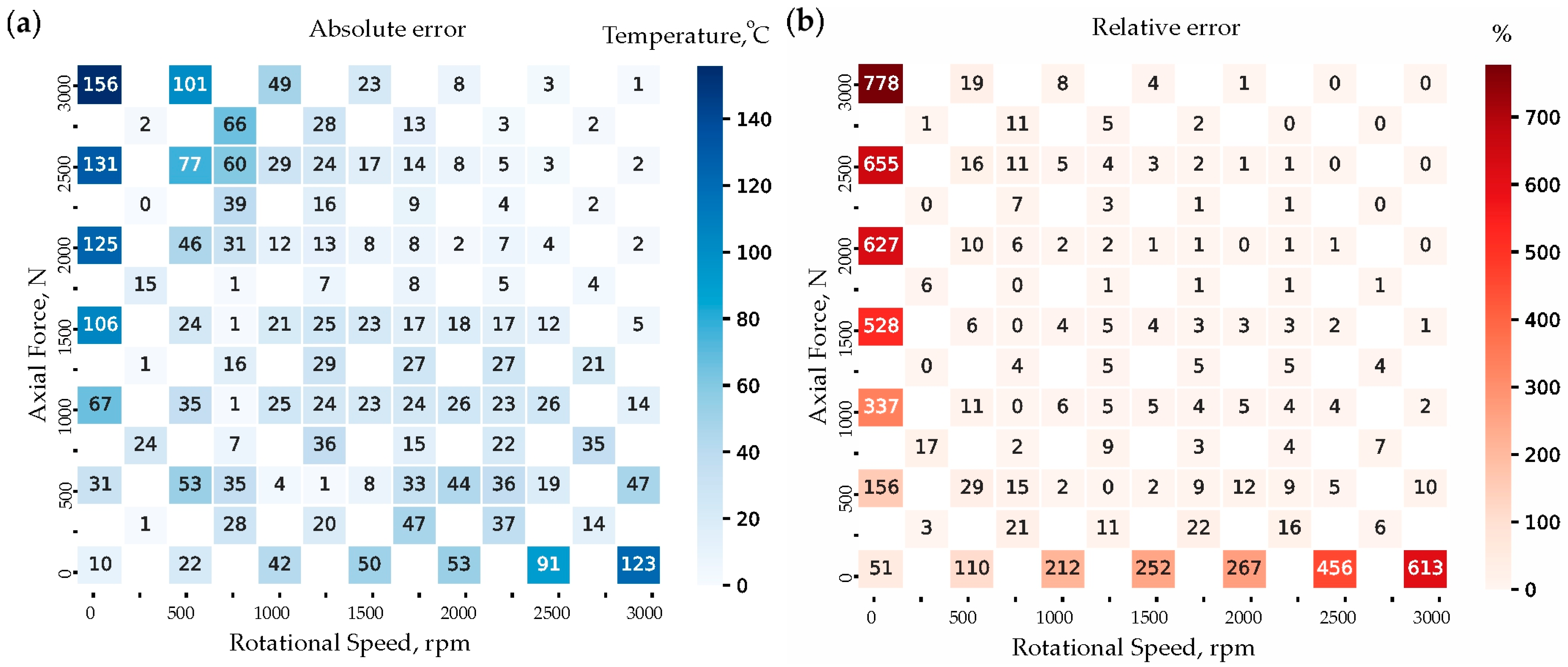
5.3. Error Analysis and Predictive Capabilities
Author Contributions
Funding
Institutional Review Board Statement
Informed Consent Statement
Data Availability Statement
Conflicts of Interest
Abbreviations
| AI | Artificial Intelligence |
| ANN | Artificial Neural Networks |
| COF | Combined Objective Function |
| CR | Crossover Rate |
| DT | Digital Twins |
| ER | Elitism Rate |
| ES | Encoding Scheme |
| F | Fitness Function |
| FEM | Finite Element Method |
| FF | Fitness Function |
| FS | Fitness Score |
| GA | Genetic Algorithm |
| HAZ | Heat-Affected Zone |
| ML | Machine Learning |
| MR | Mutation Rate |
| MSE | Mean Square Error |
| NG | Number of Generations |
| PS | Population Size |
| R2 | R-squared |
| RFW | Rotary Friction Welding |
| RSM | Response Surface Methodology |
| SM | Selection Method |
| TC | Termination Criteria |
| TS | Tournament Size |
| UTS | Ultimate Tensile Strength |
Appendix A

| Training Set (49%) | Validation Set (34%) | Test Set (19%) | |||||||||
|---|---|---|---|---|---|---|---|---|---|---|---|
| ID | X1 | X2 | Z1 | ID | X1 | X2 | Z1 | ID | X1 | X2 | Z1 |
| 1 2 3 4 5 6 7 8 9 10 11 12 13 14 15 16 17 18 19 20 21 22 23 24 25 26 27 28 29 30 31 32 33 34 35 36 37 38 39 40 41 42 43 44 45 46 47 48 49 | 3000 2500 2000 1500 1000 500 0 3000 2500 2000 1500 1000 500 0 3000 2500 2000 1500 1000 500 0 3000 2500 2000 1500 1000 500 0 3000 2500 2000 1500 1000 500 0 3000 2500 2000 1500 1000 500 0 3000 2500 2000 1500 1000 500 0 | 0 0 0 0 0 0 0 500 500 500 500 500 500 500 1000 1000 1000 1000 1000 1000 1000 1500 1500 1500 1500 1500 1500 1500 2000 2000 2000 2000 2000 2000 2000 2500 2500 2500 2500 2500 2500 2500 3000 3000 3000 3000 3000 3000 3000 | 20 20 20 20 20 20 20 468 430 385 329 270 182 20 590 575 545 514 447 310 20 622 612 594 567 522 398 20 632 632 622 610 572 455 20 632 632 630 623 592 488 20 632 632 632 632 612 520 20 | 50 51 52 53 54 55 56 57 58 59 60 61 62 63 64 65 66 67 68 69 70 71 72 73 74 75 76 77 78 79 80 81 82 83 84 85 | 2750 2250 1750 1250 750 250 2750 2250 1750 1250 750 250 2750 2250 1750 1250 750 250 2750 2250 1750 1250 750 250 2750 2250 1750 1250 750 250 2750 2250 1750 1250 750 250 | 250 250 250 250 250 250 750 750 750 750 750 750 1250 1250 1250 1250 1250 1250 1750 1750 1750 1750 1750 1750 2250 2250 2250 2250 2250 2250 2750 2750 2750 2750 2750 2750 | 240 230 210 180 135 50 520 500 460 400 300 140 600 584 560 525 435 200 624 618 600 575 500 240 632 630 623 605 550 270 632 630 630 620 575 280 | 86 87 88 89 90 91 92 93 94 95 96 97 98 99 100 101 102 103 104 105 | 2250 1750 1250 750 2250 1750 1250 750 2250 1750 1250 750 2250 1750 1250 750 2250 1750 1250 750 | 500 500 500 500 1000 1000 1000 1000 1500 1500 1500 1500 2000 2000 2000 2000 2500 2500 2500 2500 | 410 360 304 235 565 530 490 395 603 585 548 485 632 620 600 540 632 630 615 570 |
References
- Lacki, P.; Adamus, J.; Więckowski, W.; Motyka, M. A New Method of Predicting the Parameters of the Rotational Friction Welding Process Based on the Determination of the Frictional Heat Transfer in Ti Grade 2/AA 5005 Joints. Materials 2023, 16, 4787. [Google Scholar] [CrossRef]
- Lakache, H.E.; May, A.; Badji, R.; Benhammouda, S.E.; Ramtani, S. The Impact of the Rotary Friction Welding Pressure on the Mechanical and Microstructural Characteristics of Friction Welds Made of the Alloys TiAl6V4 and 2024 Aluminum. Exp. Tech. 2024, 48, 473–484. [Google Scholar] [CrossRef]
- Bauri, S.K.; Babu, N.K.; Ramakrishna, M.; Rehman, A.U.; Prasad, V.J.; Suryanarayana Reddy, M.R. Microstructural and Mechanical Properties of Dissimilar AA7075 and AA2024 Rotary Friction Weldments. Crystals 2024, 14, 1011. [Google Scholar] [CrossRef]
- Hu, M.; Zhi, S.; Chen, J.; Li, R.; Liu, B.; He, L.; Yang, H.; Wang, H. Restraint of intermetallic compound and improvement of mechanical performance of Ti/Al dissimilar alloy by rotary friction welding based on laser powder bed fusion. J. Manuf. Process. 2024, 131, 440–454. [Google Scholar] [CrossRef]
- Yaknesh, S.; Rajamurugu, N.; Babu, P.K.; Subramaniyan, S.; Khan, S.A.; Saleel, C.A.; Nur-E-Alam, M.; Soudagar, M.E.M. A technical perspective on integrating artificial intelligence to solid-state welding. Int. J. Adv. Manuf. Technol. 2024, 132, 4223–4248. [Google Scholar] [CrossRef]
- Mattie, A.A.; Ezdeen, S.Y.; Khidhir, G.I. Optimization of parameters in rotary friction welding process of dissimilar austenitic and ferritic stainless steel using finite element analysis. Adv. Mech. Eng. 2023, 15, 1–16. [Google Scholar] [CrossRef]
- Sharma, A.; Kosasih, E.; Zhang, J.; Brintrup, A.; Calinescu, A. Digital Twins: State of the art theory and practice, challenges, and open research questions. J. Ind. Inf. Integr. 2022, 30, 100383. [Google Scholar] [CrossRef]
- Negri, E.; Fumagalli, L.; Macchi, M. A Review of the Roles of Digital Twin in CPS-based Production Systems. Procedia Manuf. 2017, 11, 939–948. [Google Scholar] [CrossRef]
- Wagner, R.; Schleich, B.; Haefner, B.; Kuhnle, A.; Wartzack, S.; Lanza, G. Challenges and Potentials of Digital Twins and Industry 4.0 in Product Design and Production for High Performance Products. Procedia CIRP 2019, 84, 88–93. [Google Scholar] [CrossRef]
- Glaessgen, E.H.; Stargel, D.S. The Digital Twin Paradigm for Future NASA and U.S. Air Force Vehicles. In Proceedings of the 53rd AIAA/ASME/ASCE/AHS/ASC Structures, Structural Dynamics and Materials; Conference 20th AIAA/ASME/AHS Adaptive Structures Conference 14th AIAA, Honolulu, HI, USA, 23–26 April 2012. [Google Scholar]
- Boje, C.; Guerriero, A.; Kubicki, S.; Rezgui, Y. Towards a semantic Construction Digital Twin: Directions for future research. Autom. Constr. 2020, 114, 103179. [Google Scholar] [CrossRef]
- Attaran, M.; Celik, B.G. Digital Twin: Benefits, use cases, challenges, and opportunities. Decis. Anal. J. 2023, 6, 100165. [Google Scholar] [CrossRef]
- Więckowski, W.; Lacki, P.; Derlatka, A.; Wieczorek, P. Numerical Study of Rotary Friction Welding of Automotive Components. Adv. Sci. Technol. Res. J. 2024, 18, 336–346. [Google Scholar] [CrossRef] [PubMed]
- Nayif, A.M.; Younis, A.D.; Al Sarraf, Z.S. Investigation of the Process Parameters in Rotary Friction Welded Dissimilar AA7075/AA5083 Aluminum Alloy Joints on Fatigue Initiation using FEA and ANN. Wseas Trans. Appl. Theor. Mech. 2024, 19, 97–112. [Google Scholar] [CrossRef]
- Winiczenko, R.; Skibicki, A.; Skoczylas, P. Optimization of Friction Welding Parameters to Maximize the Tensile Strength of Magnesium Alloy with Aluminum Alloy Dissimilar Joints Using Genetic Algorithm. Processes 2021, 9, 1550. [Google Scholar] [CrossRef]
- Sreenivasan, K.S.; Satish Kumar, S.; Katiravan, J. Genetic algorithm based optimization of friction welding process parameters on AA7075-SiC composite. Eng. Sci. Technol. Int. J. 2019, 22, 1136–1148. [Google Scholar] [CrossRef]


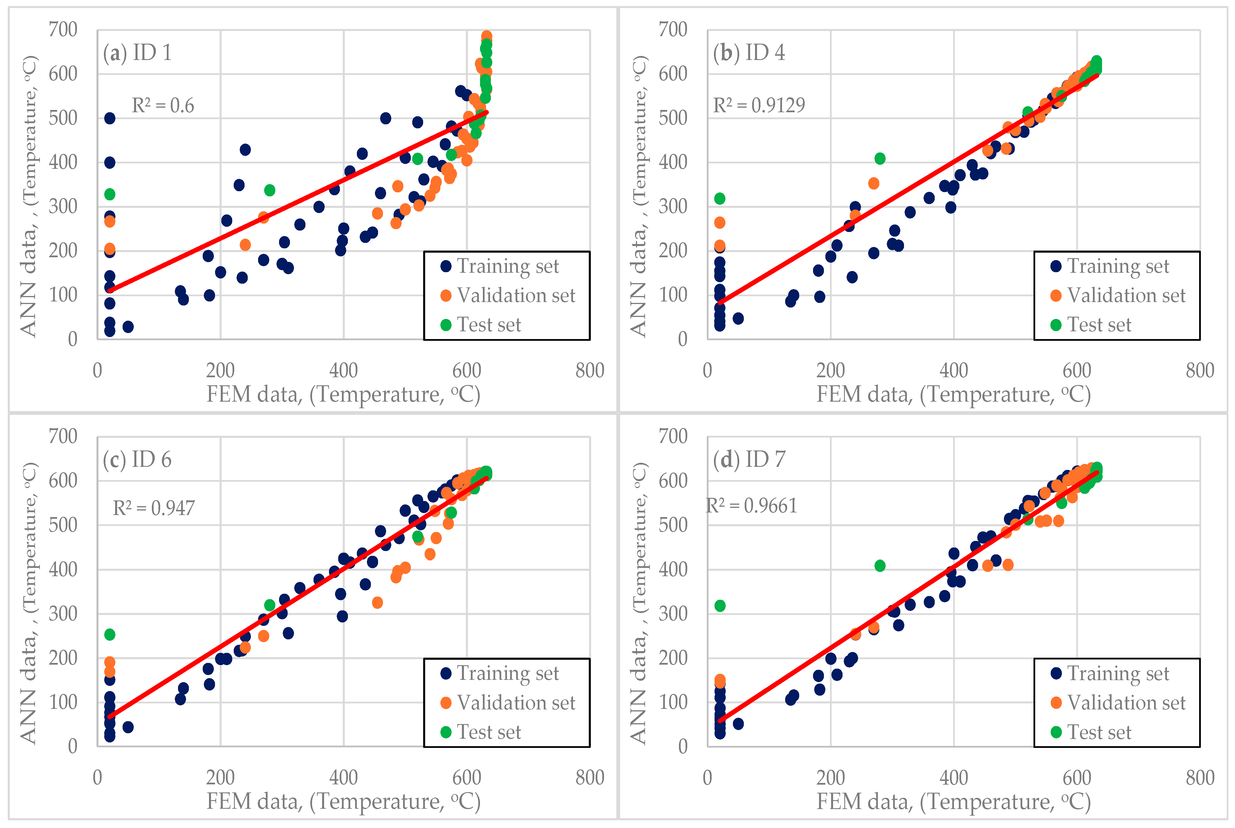


| ID | Topology | Activation Functions | Learning Rate | Epoch (All/Best) | MSE * | R2 | Training Time, s |
|---|---|---|---|---|---|---|---|
| 1 | 2-8-1 | Linear-Linear-Linear | 0.1 | 100/61 | 0.157/0.175/0.157 | 0.6 | 3.94 |
| 2 | 2-16-1 | Linear-Linear-Sigmoid | 0.01 | 100/57 | 0.135/0.147/0.136 | 0.6848 | 6.55 |
| 3 | 2-16-1 | Linear-Tanh-Sigmoid | 0.01 | 100/100 | 0.125/0.137/0.130 | 0.7329 | 6.61 |
| 4 | 2-16-1 | Linear-Tanh-Sigmoid | 0.01 | 500/485 | 0.071/0.057/0.086 | 0.9129 | 33.42 |
| 5 | 2-16-16-1 | Linear-Tanh-Tanh-Sigmoid | 0.01 | 500/210 | 0.055/0.065/0.063 | 0.9732 | 89.41 |
| 6 | 2-16-16-1 | Linear-Tanh-Tanh-Sigmoid | 0.001 | 1000/1000 | 0.054/0.056/0.055 | 0.947 | 178.87 |
| 7 | 2-16-16-1 | Linear-Tanh-Tanh-Sigmoid | 0.001 | 5000/2038 | 0.045/0.045/0.045 | 0.9661 | 946.12 |
| 8 | 2-16-16-1 | Linear-Tanh-Tanh-Sigmoid | 0.0001 | 10,000/10,000 | 0.041/0.055/0.079 | 0.9314 | 1827.32 |
| ID | F * | Constraints | Search Domain Common to All FFs | PS | NG | Hyperparameter Values Common to All FFs | ANN Record Selected by GA [n, FA, T] |
|---|---|---|---|---|---|---|---|
| A | f(n,T) = n + T | 380 < T < 600 | 60 | 10 | CR = 0.6 | [500.0, 1750.0, 398] | |
| B | f(n,T) = 1/n + T | 380 < T < 600 | 65 | 15 | MR = 0.2 | [1000.0, 750.0, 389] | |
| C | f(n,T) = 1/n + 1/T | 380 < T < 600 | 70 | 20 | SM = Tournament | [2250.0, 1000.0, 588] | |
| D | f(FA,T) = FA + T | 400 < T < 580 | 500 < n < 2500 | 80 | 25 | TS = 4 | [2500.0, 500.0, 411] |
| E | f(FA,T) = 1/FA + T | 400 < T < 580 | 500 < FA < 2500 | 85 | 30 | ER = 1% | [500.0, 2000.0, 409] |
| F | f(FA,T) = 1/FA + 1/T | 400 < T < 580 | 90 | 35 | TC = Max generations | [1000.0, 2500.0, 563] | |
| G | f(n,FA) = n + FA | 470 < T < 530 | 100 | 50 | ES = Real-valued | [1000.0, 1000.0, 472] | |
| H | f(n,FA) = 1/(n + FA) | 470 < T < 530 | 100 | [750.0, 2500.0, 510] |
Disclaimer/Publisher’s Note: The statements, opinions and data contained in all publications are solely those of the individual author(s) and contributor(s) and not of MDPI and/or the editor(s). MDPI and/or the editor(s) disclaim responsibility for any injury to people or property resulting from any ideas, methods, instructions or products referred to in the content. |
© 2025 by the authors. Licensee MDPI, Basel, Switzerland. This article is an open access article distributed under the terms and conditions of the Creative Commons Attribution (CC BY) license (https://creativecommons.org/licenses/by/4.0/).
Share and Cite
Lacki, P.; Adamus, J.; Lachs, K.; Lacki, W. Optimization of Rotary Friction Welding Parameters Through AI-Augmented Digital Twin Systems. Materials 2025, 18, 1923. https://doi.org/10.3390/ma18091923
Lacki P, Adamus J, Lachs K, Lacki W. Optimization of Rotary Friction Welding Parameters Through AI-Augmented Digital Twin Systems. Materials. 2025; 18(9):1923. https://doi.org/10.3390/ma18091923
Chicago/Turabian StyleLacki, Piotr, Janina Adamus, Kuba Lachs, and Wiktor Lacki. 2025. "Optimization of Rotary Friction Welding Parameters Through AI-Augmented Digital Twin Systems" Materials 18, no. 9: 1923. https://doi.org/10.3390/ma18091923
APA StyleLacki, P., Adamus, J., Lachs, K., & Lacki, W. (2025). Optimization of Rotary Friction Welding Parameters Through AI-Augmented Digital Twin Systems. Materials, 18(9), 1923. https://doi.org/10.3390/ma18091923