Abstract
Precisely estimating the position, diameter at breast height (DBH), and height of trees is essential in forest resource inventory. Augmented reality (AR)-based devices help overcome the issue of inconsistent global point cloud data under thick forest canopies with insufficient Global Navigation Satellite System (GNSS) coverage. Although monocular simultaneous localization and mapping (SLAM) is one of the current mainstream systems, there is still no monocular SLAM solution for forest resource inventories, particularly for the precise measurement of inclined trees. We developed a forest plot survey system based on monocular SLAM that utilizes array cameras and Inertial Measurement Unit (IMU) sensors provided by smartphones, combined with augmented reality technology, to achieve a real-time estimation of the position, DBH, and height of trees within forest plots. Our results from the tested plots showed that the tree position estimation is unbiased, with an RMSE of 0.12 m and 0.11 m in the x-axis and y-axis directions, respectively; the DBH estimation bias is −0.17 cm (−0.65%), with an RMSE of 0.83 cm (3.59%), while the height estimation bias is −0.1 m (−0.95%), with an RMSE of 0.99 m (5.38%). This study will be useful in designing an algorithm to estimate the DBH and position of inclined trees using point clouds constrained by sectional planes at the breast height of the trunk, developing an algorithm to estimate the height of inclined trees utilizing the relationship between rays and plane positions, and providing observers with visual measurement results using augmented reality technology, allowing them to judge the accuracy of the estimates intuitively. Clearly, this system has significant potential applications in forest resource management and ecological research.
1. Introduction
Forests are indispensable in the Earth’s ecosystem, providing habitats for various species, regulating the climate, storing carbon [1,2,3], and similarly offering a wealth of ecosystem services, such as timber, non-timber forest products, and recreational opportunities [1,2,3]. Additionally, forests are vital for human welfare, providing energy, building materials, and food [4]. A forest resource inventory enables the collection of forest resource data, laying the foundation for the planning and monitoring of sustainable forest management [5]. The forest plot survey is a crucial method for forest resource inventories [6], typically involving collecting tree data through individual tree measurements [7,8,9,10]. The primary data collection includes tree position, DBH, and height [11,12,13]; this information is widely used to predict other essential tree attributes such as age, volume, biomass, and carbon storage, which non-destructive methods cannot accurately measure [14]. In addition, real-time measurement can provide immediate data, allowing fields such as forest management, environmental monitoring, and urban planning to make more agile decisions and respond to changes promptly.
Traditional forest resource surveys involve manual measurements using mechanical or optical instruments such as calipers, compasses, and rangefinders [15,16]. However, these conventional techniques are time-consuming, expensive, and prone to measurement errors [17,18]. In recent years, Terrestrial Laser Scanning (TLS) systems have been successfully applied in forestry [7,19,20,21,22]. The main advantage of TLS is its ability to measure digitized forest detail accurately, quickly, and automatically, with millimeters of error level [23,24], and on the other hand, enabling precise estimation of the main attributes of trees [25]. However, due to the static nature of TLS [26], single-scan modes suffer from severe occlusion issues [27], multi-scan modes are time-consuming [28], and the high cost of TLS inhibits forest resource surveys [29]. Forest surveying through mobile laser scanning (MLS) overcomes the static nature of TLS and reduces occlusion effects [30], serving as an alternative to TLS [31]. MLS used a laser scanner with an Inertial Measurement Unit (IMU)GNSS, with the quality of its point clouds being influenced by the accuracy, precision, and synchronization of these three components [32]. However, dense tree canopies obstruct GNSS signals, preventing MLS from constructing globally consistent point clouds [33,34]. Simultaneous localization and mapping (SLAM) is a technology for autonomous positioning and mapping in unknown environments using sensor data [35,36]. The advent of SLAM algorithms reduces reliance on GNSS signals [37], offering a potential solution. Nowadays, SLAM technology is integrated into personal Light Detection and Ranging (LiDAR) systems [18,38], enabling scanners to achieve precise positioning in forest environments where GNSS signals are obstructed [39]. However, the point cloud accuracy of this system is relatively low, compounded by challenges in SLAM matching during field operations, resulting in the limited application of PLS in forest resource inventory.
With significant advancements in computing capabilities and sensor technologies, consumer-grade array cameras, ToF cameras, LiDAR, and IMUs have been integrated into mobile devices [40]. SLAM algorithms such as Tango, ARCore, and ARKit can run on mobile devices, supporting the implementation of augmented reality. Tango is a technology platform developed by Google; it combines advanced sensors, cameras, and computational power, enabling devices to perceive and understand their surroundings in real-time and collect 3D data [41,42]. This technology has been widely used by researchers in forestry [43], who have tested its accuracy for tree position and DBH in circular plots. On the other hand, the authors of [44,45] accurately tested the observation procedures and algorithms for tree position, DBH, and tree height, building an RGB-D SLAM portable tree-measuring system for single-tree and forest plot surveys. However, starting in 2018, Google announced discontinuing support for the Tango platform, shifting its focus to other augmented reality technologies like ARCore and ARKit, which are more general augmented reality solutions that do not require special hardware [40], have the demerit of weaker precision in acquiring 3D data, but offer advantages in device compatibility and popularity. Fan et al. were among the first to use this approach to design precise estimation algorithms for DBH and tree position, and they constructed a monocular SLAM augmented reality forest tree-measuring system, achieving the real-time monitoring of measurement results [40]. Due to its high estimation accuracy and robustness, this system is a potential solution for precise forest plot surveys [40]. But still, it is unsuitable for accurately estimating inclined trees’ DBH, position, and height. Furthermore, there is no established comprehensive forest plot survey system.
This paper aims to estimate forest attributes in real time in a forest inventory using a mobile phone with monocular SLAM technology. The main objectives of this research are (i) to develop a forest plot survey system for smartphones with a monocular SLAM system; (ii) to develop an algorithm for estimating the DBH and position of trees, utilizing point clouds constrained by sectional planes’ DBH, addressing the challenge of accurately estimating inclined trees; and (iii) to design an algorithm for estimating the height of inclined trees using the relationship between rays and plane positions.
2. Protocols and Mechanism
2.1. Monocular SLAM Theory
SLAM technology is a crucial research area in autonomous robots and automated systems, addressing the complex problem of self-localization and environmental mapping in unknown environments [35]. In SLAM systems, state estimation is fundamental and is typically achieved through Bayesian filters, such as the Extended Kalman Filter (EKF) or Particle Filter [44]. These filters combine motion models and observation models to estimate the state. The monocular SLAM system in this research uses an array camera as the observation model and an IMU as the motion model. The motion model describes how the device moves and is typically represented as:
Here, is the state at time t, is the control input (such as velocity and direction), and is the process noise. The observation model describes how to generate observation data from the current state, represented as:
where is the observation value and is the observation noise. The SLAM process integrates camera observation data with IMU data and performs a real-time estimation of the pose and observation data at each moment, represented as Equation (3):
The mathematical foundation of SLAM technology is based on probability theory and estimation theory [44]. Bayesian filters are at the core of SLAM, using an equation for state estimation; see Equation (4):
where represents the posterior probability of the state, given all observations and control inputs.
Monocular SLAM is one of the mainstream SLAM systems today [46], consisting of a camera and a low-cost IMU for measuring the smallest suite of sensors for six-degree-of-freedom state estimation. This configuration meets the requirements of most smartphones. ARCore, the augmented reality platform launched by Google, has been integrated into most current Android smartphones without the need for special hardware support, providing high scalability and portability [40]. Therefore, in this paper, we chose to use an Android smartphone that meets the above requirements to build a forest plot survey system.
As shown in Figure 1, the implementation of monocular SLAM typically consists of modules, i.e., data preprocessing, initialization, non-linear optimization based on a sliding window, loop closure detection, and pose graph optimization [46]. In the data preprocessing stage, images undergo Harris corner extraction and pyramid optical flow tracking. However, the outliers are removed using the RANSAC algorithm, and the tracked feature points are added to the image queue for backend processing. Concurrently, IMU data are processed through an integration providing pose information such as position, velocity, and rotation. The pre-integration increment, its Jacobian matrix, and covariance are calculated, providing the necessary data for subsequent optimization. During the initialization stage, the system performs a pure visual estimation using SFM (Structure from Motion) technology, estimating the pose of all frames within the sliding window and the inverse depth of 3D landmark points. The SFM is loosely coupled with IMU pre-integration, working to align and solve the initialization parameters. However, in the non-linear optimization stage based on the sliding window, the system integrates visual IMU and loop closure constraints into a significant objective function for non-linear optimization, solving for the pose and bias of all frames within the sliding window. Loop closure detection is conducted by using the DBow (Distributed Bag of Words) algorithm. Once a loop is successfully detected, the system relocalizes and optimizes the camera trajectory to enhance the accuracy of the trajectory estimation. Finally, pose graph optimization ensures the global optimization of historical poses based on the relocalization results, further strengthening the system’s stability and accuracy.

Figure 1.
The implementation process of monocular SLAM.
2.2. Monocular Densification Reconstruction
Although the system in this paper does not require special hardware support, only sparse point cloud information can be obtained during the environment-understanding process. This poses a great challenge for designing DBH and location estimation. In order to reduce the estimation difficulty and error due to insufficient point cloud information, the environment information needs to be densified.
The core of monocular densification is to enhance environmental understanding by estimating depth maps [40]. This process relies on the pose and sparse map information provided by SLAM. Based on the Lambertian surface assumption, which states that the intensity of light reflected by a surface only depends on the angle of incidence, and the photometric consistency assumption that maintains the intensity of light on the same surface and states that it should be consistent from different viewpoints combined with visibility constraints, a photometric consistency non-linear optimization model was constructed [47,48]. This model can be represented as:
Here, represents the sum of photometric residuals between the current frame and multiple surrounding frames; is the photometric value of the pixel in the recent Patch in the reference frame (the current frame); represents the photometric value of the pixel in the corresponding Patch of the k-th frame; and is the color scale of the k-th frame. This model focuses on the photometric differences of the pixels, comparing the photometric values of a small section (Patch) in the current frame with those of the corresponding section in previous frames. The photometric differences of these pixels are accumulated into a total residual value. By minimizing the sum of squares of these photometric residuals, the depth of the central pixel in the current Patch can be estimated and further expanded to generate the entire depth map and its confidence map using region-growing techniques. When applied to specific scenarios such as estimating the depth maps of tree trunks in forests, this method allows the conversion of the obtained depth maps into point clouds, further enabling the estimation of the position and DBH of the trees.
3. Materials and Methodology
3.1. System Workflow
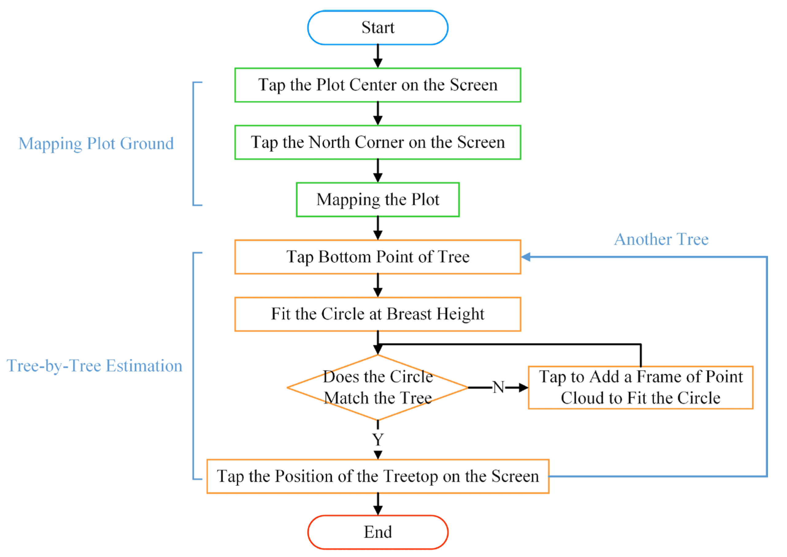
An Android application for forest plot surveys was developed to enable SLAM mobile phones to be used for forest inventory. The application uses augmented reality technology, combining an array camera as the observation sensor and an IMU as the motion sensor. In this, the array camera exhibits more minor errors in long-duration and long-distance pose estimation. At the same time, the IMU shows a higher accuracy in short-duration and short-distance pose estimation, maintaining reliability even in rapidly changing conditions [40]. The fusion of these two types of sensor data adequately compensates for their shortcomings and will be a mainstream method in SLAM systems. Based on this system, plotting a plot map and the individual tree estimation are achieved (Figure 2). The system initially needs to construct a plot map by establishing a coordinate system at the center of the plot, drawing plot boundaries, and adjusting and standardizing global coordinates. Subsequently, each tree’s position, DBH, and height are estimated and recorded according to the algorithm designed.
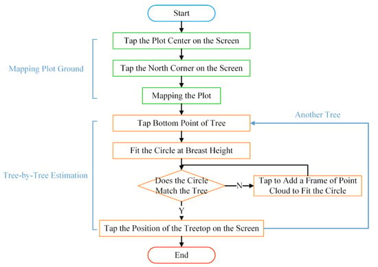
Figure 2.
The workflow of the forest plot survey system.
3.2. DBH and Tree Position Algorithm
An algorithm is established to estimate the DBH and position of individual trees by using point clouds collected at the breast height of trees as the primary data source. This method applies to both vertical and inclined trees. Initially, the model is constructed based on several key assumptions: (1) the tree is assumed to be a cylinder below breast height, which may be either vertical or inclined, and this assumption provides a basic geometric model for representing the tree; (2) the cutting plane can be formed from the camera’s center to one side of the cylinder, which is crucial for understanding and measuring tree data; (3) the cutting plane from the camera center to one side of the cylinder is considered a planar constraint for the tree, which will help to define and understand the spatial positioning of the tree; and lastly (4) the planar constraints at both ends help to form an overall constraint for the cylinder, aiding in a more accurate understanding and estimation of tree parameters.
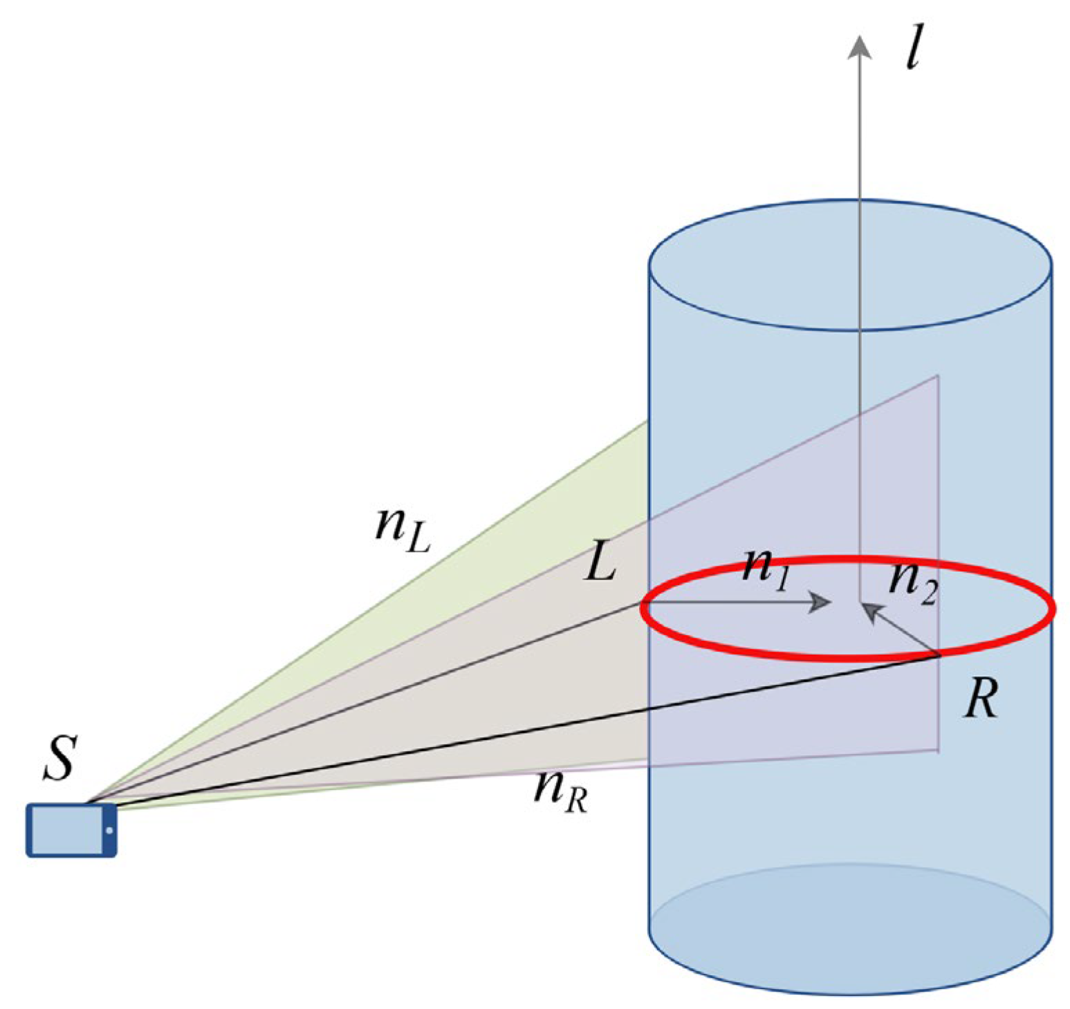
Figure 3 shows the vector relationships during tree diameter and position estimation, where the red circle represents the DBH to be measured, and represents the camera center and and are the left and right cutting points at breast height, while and are the cutting planes corresponding to these points, and are the normal vectors corresponding to the cutting planes, and is the normal vector of the tree, i.e., the unit vector of the tree’s growth direction.

Figure 3.
Vector relationship diagram in estimation of DBH and position.
Subsequently, the algorithm proceeds in several steps. First, the cutting plane and breast height data are obtained via the depth map; the breast height is acquired through user interaction, by capturing two points sequentially at the tree base point and the approximate breast height. After that, a line segment with the starting point at the tree base and a length of 1.3 m is rendered, based on the vector direction formed by these two points (the direction of the vector), with the end of the line segment indicating the breast height position, as shown in Figure 4a. Figure 4a illustrates the rendering status during the DBH measurement process. The blue line represents the 1.3 m line segment, with the end of the blue line indicating the breast height position.

Figure 4.
Rendering status during measurement of DBH. (a) single-frame fitted DBH; (b) multi-frame fitted DBH.
Next, the measurement of DBH includes both single and multiple measurements. Single measurements involve the estimating from data of a single frame point cloud, ideal for near-circular trees, as shown in Figure 4a, while multiple measurements involve collecting point cloud data from different orientations of the tree for a comprehensive estimation, which is suitable for non-circular trees, as in Figure 4b, where the direction of the angle intersecting with the circle represents an observation point, with three observations in total. For the estimation of and in single measurements, the following vector relationships apply:
Utilizing the characteristic of the IMU’s slight angle drift relative to position drift, the tree’s normal vector is estimated. In single measurements, using the vector formula is followed:
Here, represents the transformation matrix from the world coordinate system to the image polar coordinate system. In multiple measurements, each measurement from different orientations follows the following vector formula:
While estimating the DBH based on the results of single measurements, we first establish a temporary coordinate system with as the z-axis. In this coordinate system, the origin is the origin of the camera coordinate system, is the z-axis, the y-axis direction is the direction represented by , i.e., the direction from to in Figure 3, and the x-axis forms a right-hand system with the y- and z-axes. The world coordinate system is converted to the temporary coordinate system through the transformation coefficients shown in Equation (10):
After that, the point cloud data are transformed into this temporary coordinate system, using a filter (Equation (11)) to select the point cloud near the breast height position and setting the z-axis value of each transformed point to 0. Within the and planes, the diameter and position data are obtained using a circle fitting method. The resulting state received in the augmented reality scenario is shown in Figure 4.
For estimating the tree’s position, the following points must be considered: (1) there might be drifting in the position data, (2) the result of the previous step’s fitting might be a point on the axis, not the actual position, and (3) for inclined trees, the estimation of the tree position is based on the ground diameter position, i.e., the center of the point where the tree contacts the ground. To achieve this goal, we first transform the tree position estimated in the temporary coordinate system to the world coordinate system, and according to the direction of the normal vector and the ground point elevation , obtain the intersection points of different observation points with the ground. Finally, the mean of these intersection points is taken as the final position of the tree, as shown in Equation (12).
Here, is the number of measurements, and is the result of the i-th measurement.
3.3. Tree Height Algorithm
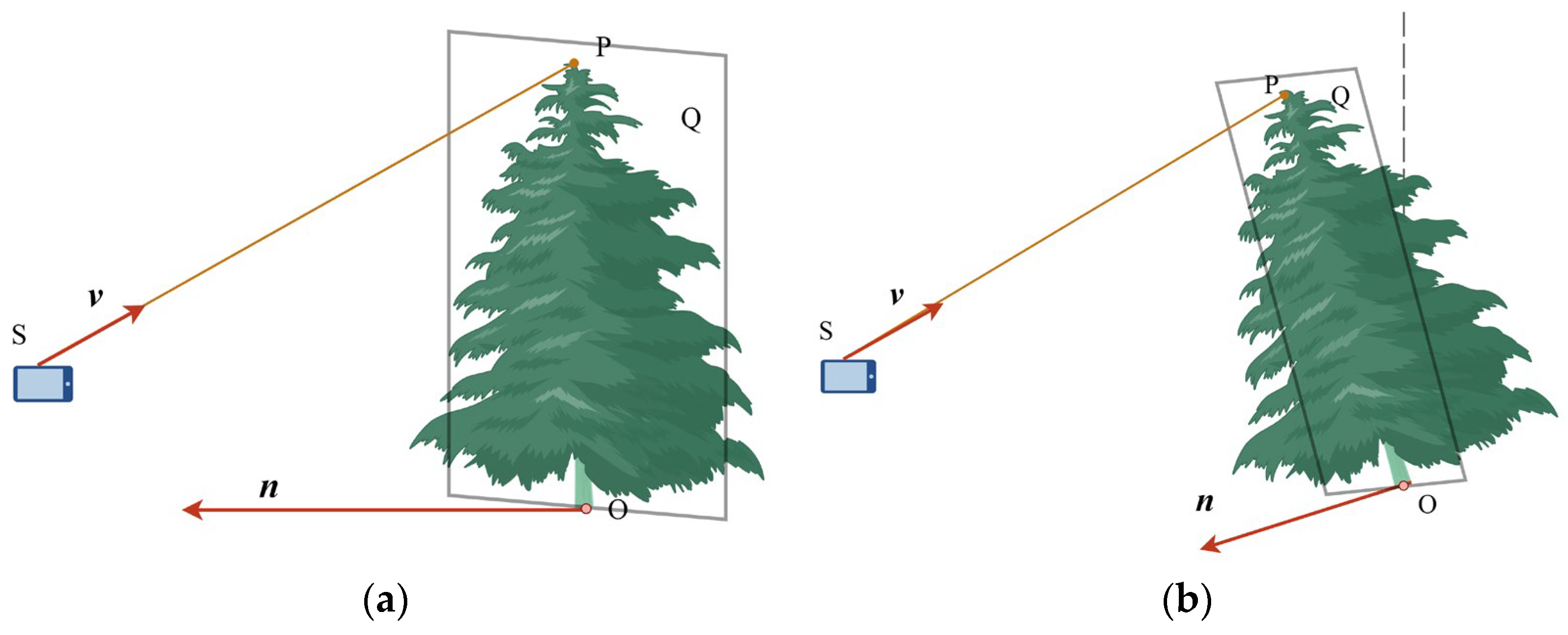
In the coordinate system of the SLAM system, the y-axis is always vertically upwards; this research sets the z-axis as vertically upwards, and therefore, by subtracting the z-coordinate of the treetop in augmented reality from the z-coordinate of the tree base, the resulting difference gives the height of the tree (the difference in z-coordinates of points and in Figure 5a). The conversion in inclined trees is necessary and is achieved by converting the coordinate system to a temporary coordinate system, with the tree trunk direction as the z-axis, as shown in Equation (10) in Section 2.2. For measuring an individual tree, the user obtains the base coordinates by tapping a point at the bottom of the tree. Therefore, the main task in determining tree height is to find the coordinates of the treetop point . The user needs to move to a position where they can observe the top of the tree, aim the camera at the treetop, and tap the treetop point on the screen. When tapping, the device emits a ray with a known starting point and direction. The starting point of the ray is the device’s position in the augmented reality coordinate system at that time, and the ray’s direction vector is denoted as so that point can be obtained as represented in Equation (13).
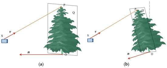
Figure 5.
Geometric relationships in tree height calculation, where is a point at the base of the tree; is the optical center of the camera; is the direction vector of ray ; is the plane facing point and parallel to the direction of the tree trunk; is the intersection of the ray and the plane; and is the normal vector on the plane passing through point . (a) Vertical tree; (b) inclined tree.
Here, is a parameter so that the ray will strike a plane parallel to the y-axis and face the device, with the normal vector of the plane passing through the tree base point as . Since plane faces the device, can be represented as in Equation (14):
Currently, the intersection of the ray and the plane is , and is a point on plane ; then, it satisfies the equation:
Combining Equations (13)–(15), the parameter and the coordinates of point can be obtained. Therefore, the tree height can be estimated as in Equation (16). After completing the tree height calculation, a line segment from the bottom of the tree to the top of the tree is rendered in the augmented reality scene, which is available for the user to monitor the accuracy of the results.
4. Test Cases
4.1. Research Area and Test Data
The study was conducted in Beijing Olympic Forest Park, situated in Beijing (116°23′2.98″ E, 40°01′3.00″ N). The park is characterized by a river alluvial plain geologic structure spanning over 680 hectares (ha), with green belts having an area of 478 hectares (ha) and with a total green cover of 95.61%. As a vital component of urban greening, the park’s vast area and lush greenery are ideal for citizens’ recreation, fitness, and nature observation. The park has diverse forest types, over 100 tree species, 80 shrub species, and over 100 herbaceous plants, forming a biodiversity-based natural forest system. Such an environment provides an ideal experimental site for the study.
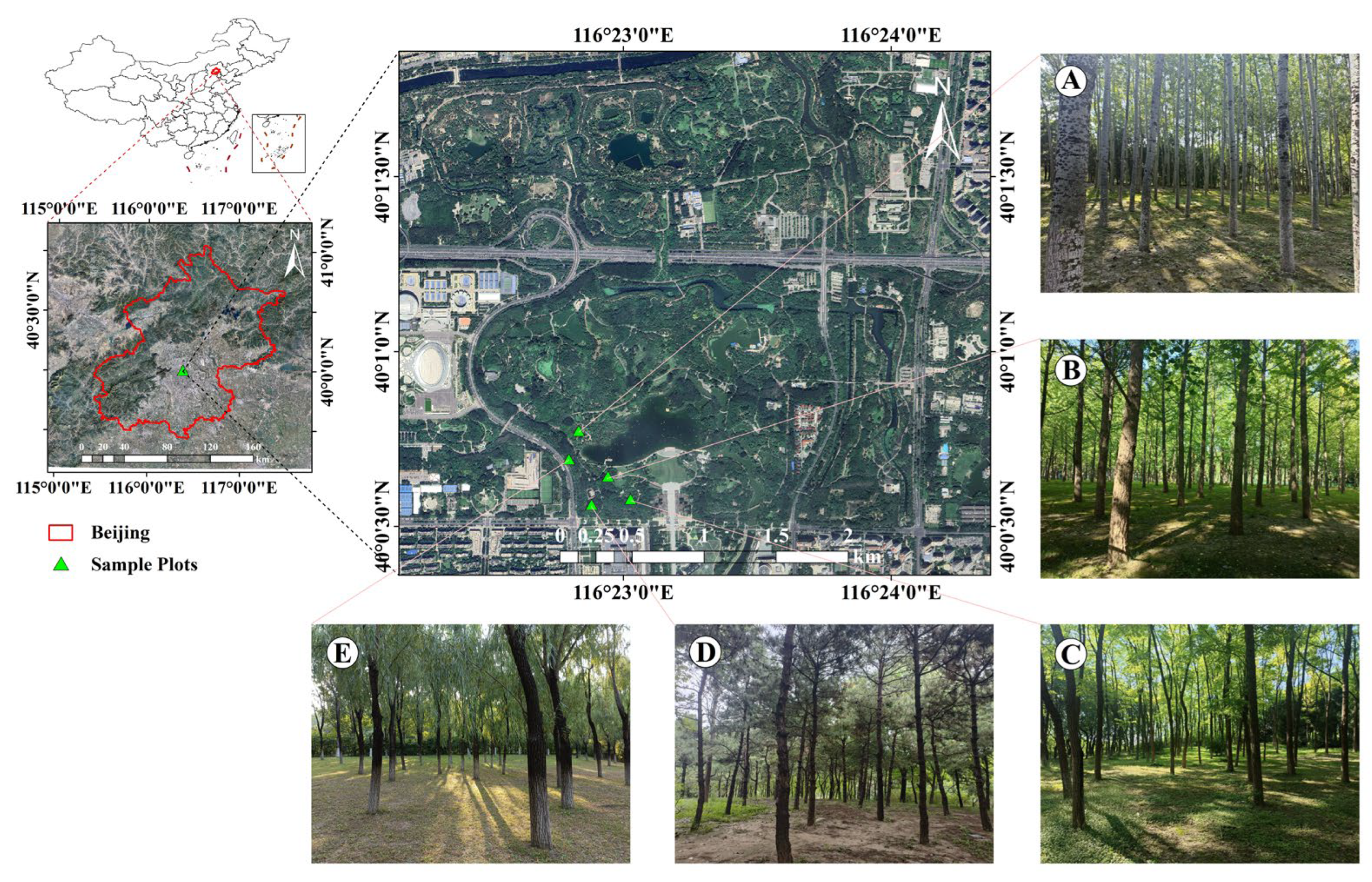
To ensure an adequate sample size and plot diversity, this research was conducted in 12 circular plots, each with a radius of 7.5 m (the area of each plot was 177 square meters), in the research area. The selection of these plots represents different forest types in terms of tree species composition, age, and stem density. We selected five tree species (Figure 6): Populus tomentosa, Ginkgo biloba, Styphnolobium japonicum, Pinus tabuliformis, and Salix matsudana. The selected plots had fewer shrubs and were accessible to locals. The position, DBH, and height of each tree in these plots were recorded, with the attributes of the plots, as shown in Table 1. The number of trees in each test plot varied from 11 to 19; the average DBH of each study plot ranged from 16.7 cm to 28.5 cm; and the average tree height ranged from 9.6 m to 25 m. Figure 7 is the probability density function of diameter at breast height and tree height in the 12 circular plots.
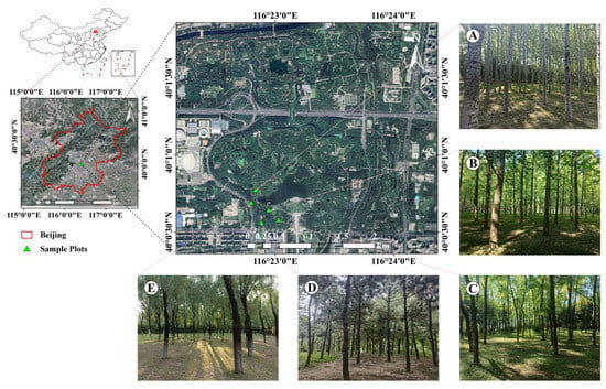
Figure 6.
Location of study area: (A) (Populus tomentosa plot), (B) (Ginkgo biloba plot), (C) (Styphnolobium japonicum plot), (D) (Pinus tabuliformis plot), (E) (Salix matsudana plot).

Table 1.
Summary statistics of plot attributes.

Figure 7.
Probability density functions for DBH and tree height for different plots. (a) DBH; (b) tree height.
4.2. Plot Inventory Procedure
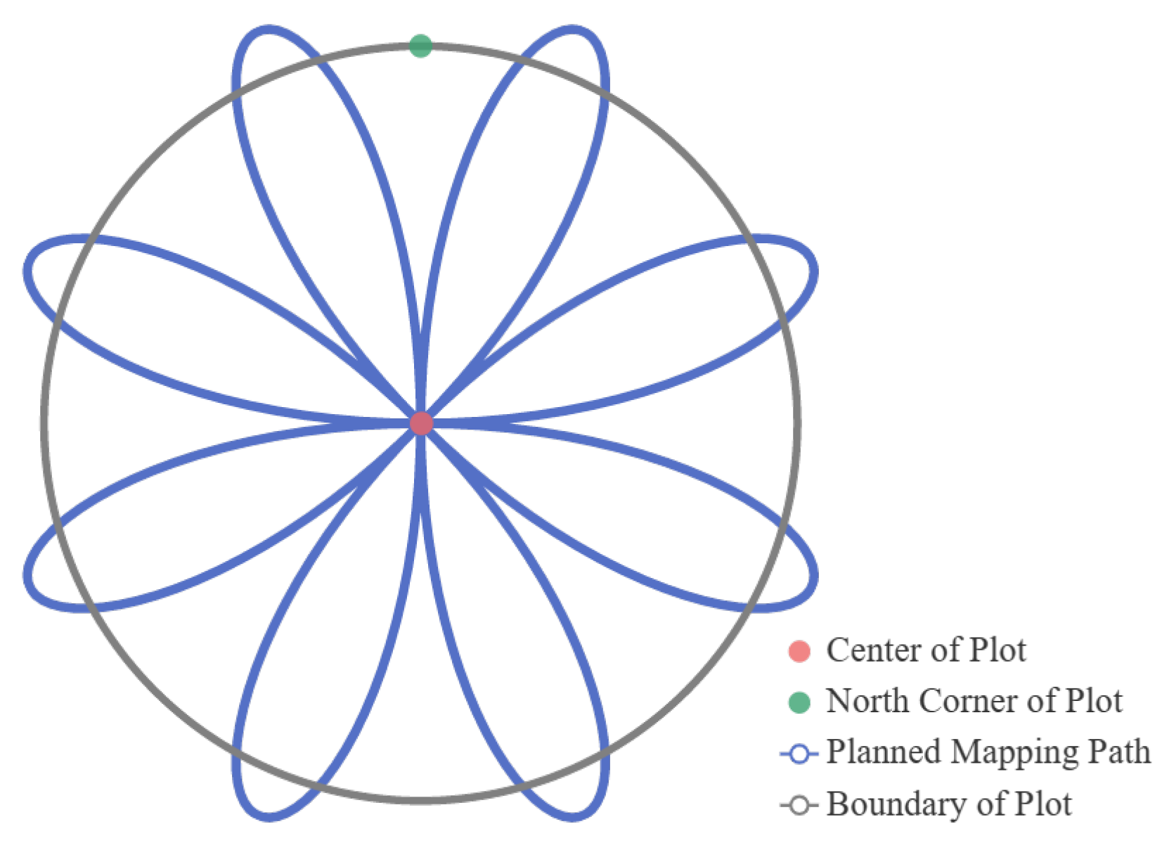
This study experimented with a circular plot with a diameter of 7.5 m (the area was 177 m2). The measurement route of the plot was the sunflower path (see Figure 8). This path starts from the center of the plot, heading towards the north, and then measures the trees in each petal area in a clockwise direction, returning to the plot’s center after measuring one petal area. To ensure the exact position of the plot center, a marker (an object used for marking) is typically placed at the plot center before starting the measurement task, with the marker pointing towards true north (Figure 9a). This research also uses an array camera as the observation sensor. However, global position optimization is performed by recognizing the marker each time the plot center is passed. Therefore, the sunflower path optimizes the position by passing through the plot center multiple times and obtaining a globally consistent plot map.
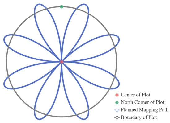
Figure 8.
Mapping path of survey plot.
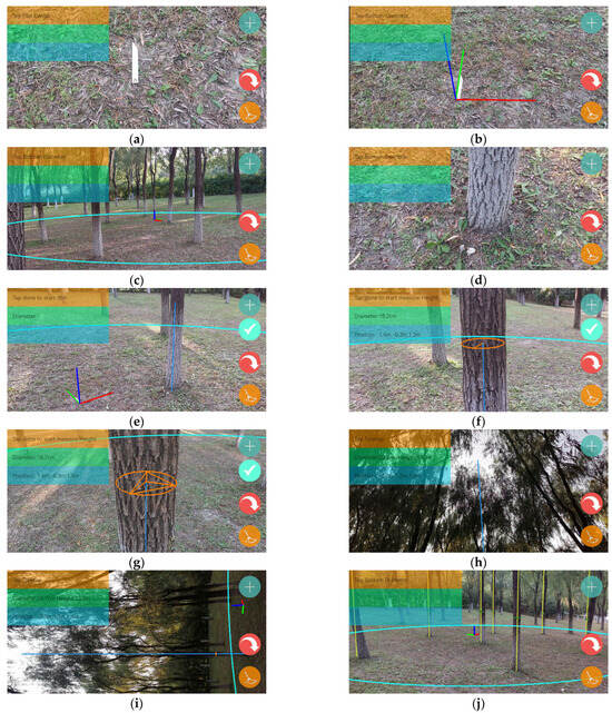
Figure 9.
System operation steps: (a) placement of markers; (b) placement of axes; (c) drawing of plot boundaries (draw with a cyan line); (d) tap bottom of tree; (e) drawing the chest-height line (draw with a blue line); (f) single-frame fitted DBH (draw with a orange line); (g) multi-frame fitted DBH; (h) tap top of tree to estimate tree height (draw with a blue line); (i) tree height panorama; (j) results of completed plot surveys (draw with a yellow line).
Figure 9 describes the measurement steps of the forest plot survey application described in this paper. Generally, SLAM systems use the first frame position of the device at application startup as the global coordinate origin. Still, this approach is unsuitable for managing plot tree positions. Therefore, before measuring each tree, we first establish a coordinate system at the plot center (Figure 9b) to move the coordinate zero point to the plot center, making it more convenient to record tree positions. After establishing the coordinate system, the system draws the plot boundaries according to the plot center (Figure 9c). Next, follow the measurement path for measuring each tree, tap the base of the tree on the screen (Figure 9d), determine the breast height position of the tree (Figure 9e), and then fit the DBH based on the single-frame point cloud at the breast-height position (Figure 9f). If the fitted circle does not match the tree trunk boundary, fit the circle by adding extra frames in different directions from the trunk (Figure 9g). Subsequently, move to a position where the treetop is visible and tap the treetop point on the screen to estimate the tree height (Figure 9h). Repeat steps d to h to complete the measurement task for all trees in the plot (Figure 9j).
4.3. Accuracy Assessment and Evaluation
This paper measures the DBH by using a diameter tape as a reference value, and the total station (Leica Flexline TS06plus, South Surveying & Mapping Technology Co., Ltd., Guangzhou, China) was used to measure trees’ precise position and height as reference values (the total station, with its laser ranging technology, can achieve precise measurements under various terrain conditions). The reference value for the DBH of inclined trees is measured with a diameter tape 1.3 m above the ground, on a plane perpendicular to the direction of the tree trunk, not in a direction parallel to the horizontal plane. When measuring the position of trees, the total station is set up at the center of the plot. The total station measures and records the angle between the center point of the tree at breast height and true north, as well as the horizontal distance from this center point to the center of the plot. For trees obstructed from view, we moved the total station a fixed distance towards true north and set a second measurement point. Then, the actual position of the tree is calculated based on the distance and angle, serving as a reference value; the reference value data were used to verify the accuracy and feasibility of the system. The bias (BIAS), root mean squared error (RMSE), relative bias (relBIAS), and relative root mean squared error (relRMSE) were used to assess the deviation and variability of each measurement value, with the following calculation formulas:
Here, is the measured value, is the corresponding reference value of the measured value , and is the total number of measured values.
4.4. Experimental Results
4.4.1. Tree Position
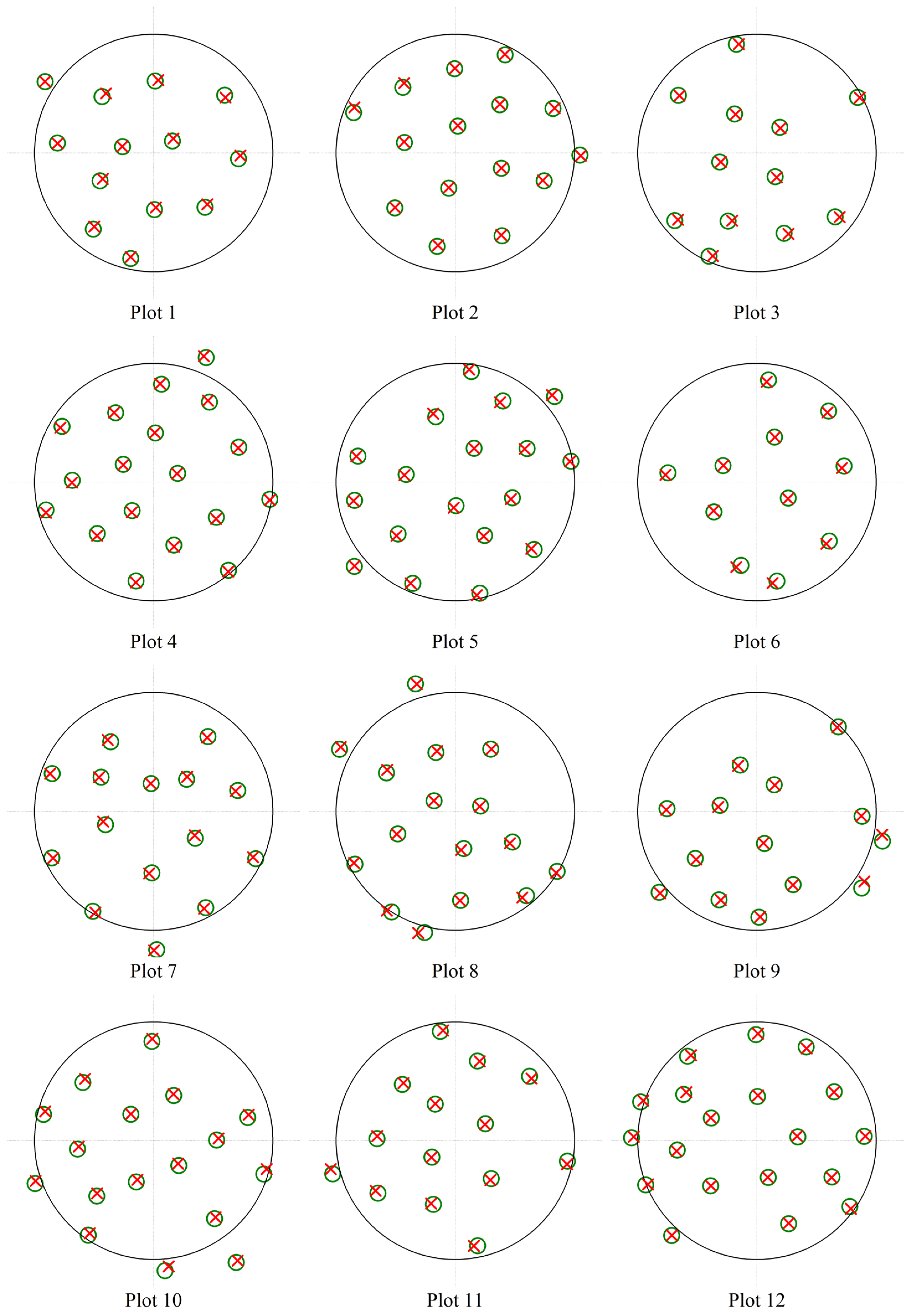
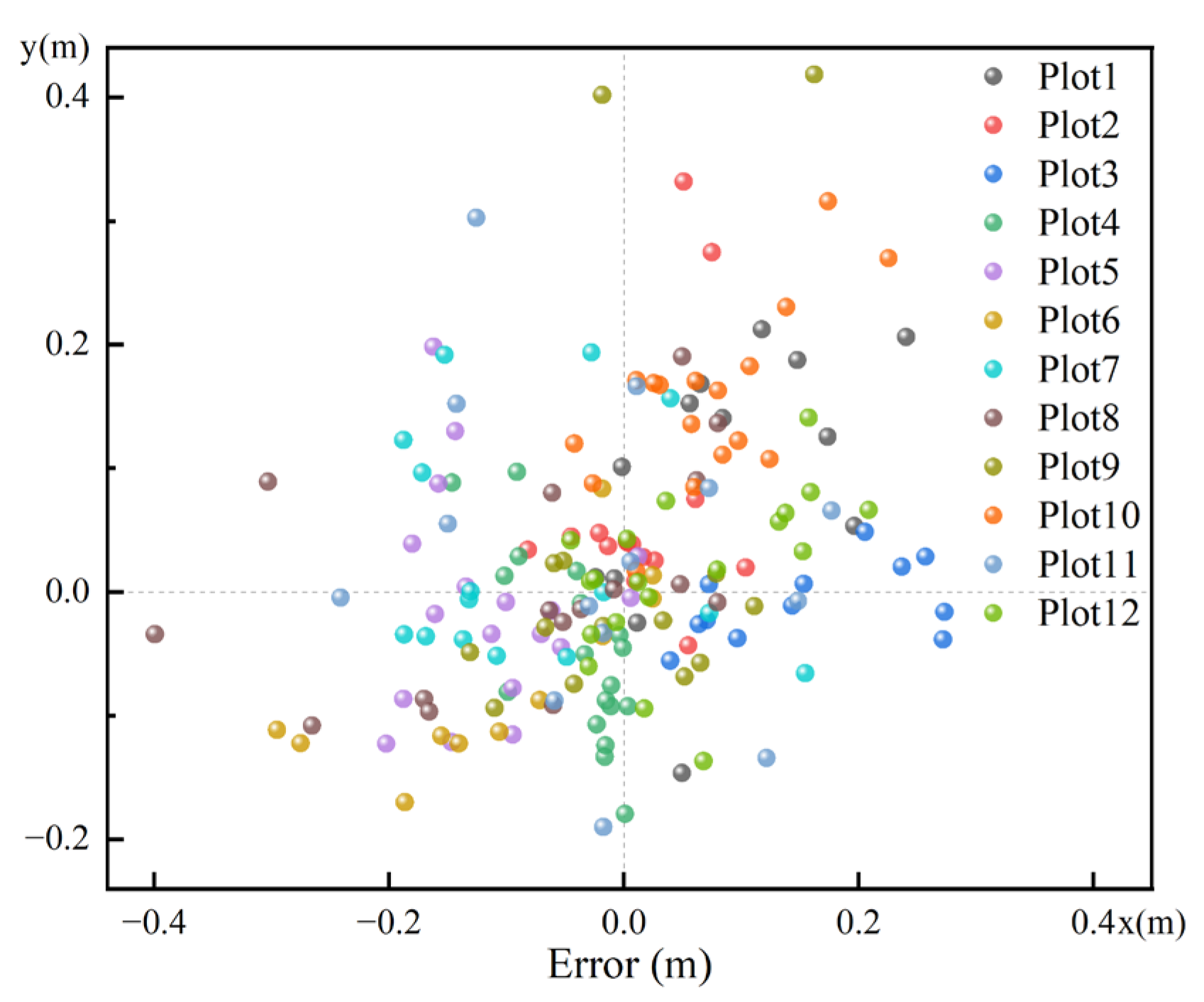
The results showed an average error range in the x and y directions of about −0.11 m to 0.16 m. Table 2 examines the average bias and root mean squared error in the x and y directions. The average X-BIAS for each plot ranged from −0.11 m to 0.16 m, with an overall average of −0.01 m, while the average Y-BIAS ranged from −0.07 to 0.15, with an overall average of 0.03 m. These results indicate some systematic biases in the estimated stem positions relative to their actual positions, but they are relatively small. The average values of X-BIAS and Y-BIAS are close to zero, which is a positive sign. The average X-RMSE is 0.12 m, while the average Y-RMSE is 0.11 m. The RMSE values are relatively consistent in the X and Y directions, suggesting a uniform error distribution. Figure 10 and Figure 11 show the position errors for all plots. Although systematic errors exist in the estimated tree positions for each plot, the overall errors are minor, and the systematic errors vary randomly across different plots.

Table 2.
Accuracy of stem position estimations.
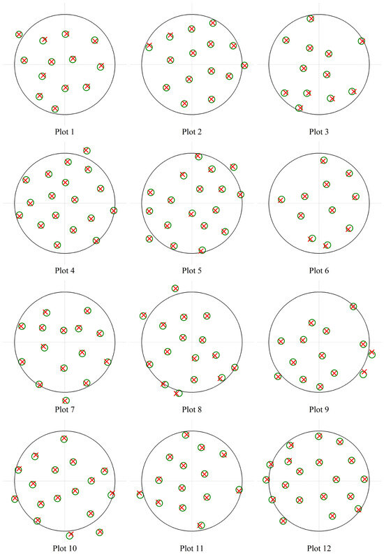
Figure 10.
The estimated and reference stem positions: the green circles indicate the stem references; the red crosses indicate the estimations.
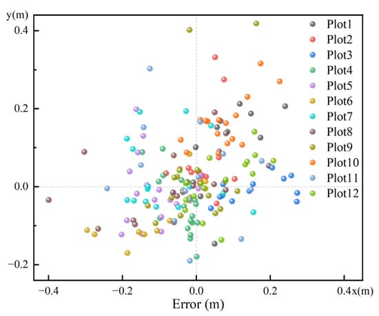
Figure 11.
The position errors of all trees in the plots.
4.4.2. Estimating DBH
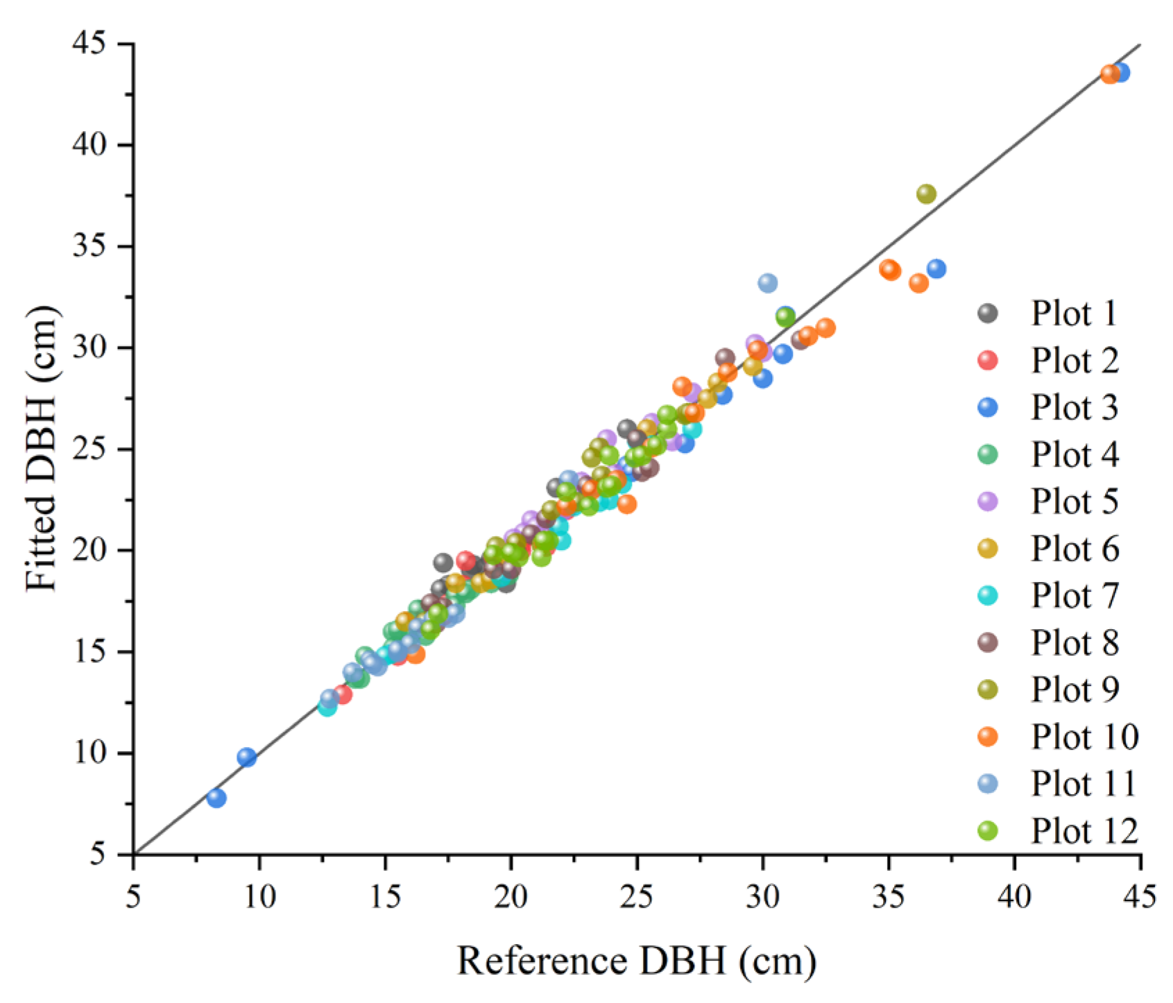
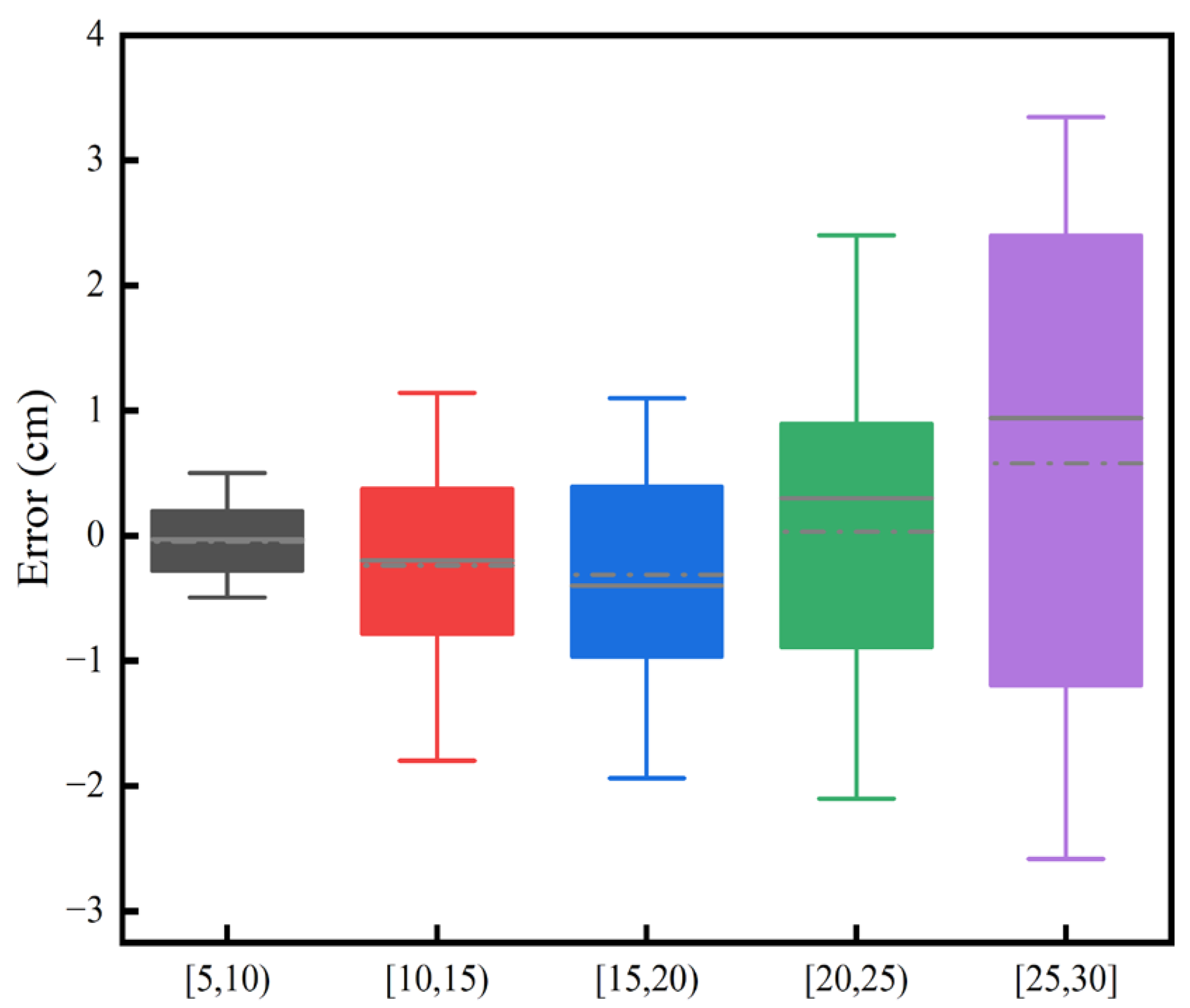
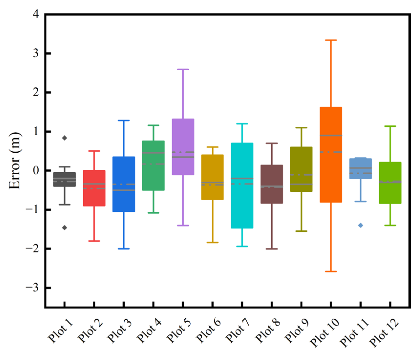
The DBH shows a BIAS that ranged from −0.78 cm to 0.61 cm, with the relative BIAS fluctuating between −2.98% and 3.22%, Table 3. The values of RMSE ranged from 0.46 cm to 1.24 cm, with the range of the relative RMSE being 2.33% to 5.3%. There is some deviation in the DBH estimation, but the percentage changes in relative bias and relative RMSE are within the limits. The RMSE also remains relatively low in different contexts, indicating a relatively high level of estimation accuracy. Figure 12 and Figure 13 indicate that the dispersion of measurement errors and observed values increases with the increase in DBH. Figure 14 shows that the error distribution between each plot’s measured and reference values is relatively uniform, and the distribution is random.

Table 3.
Accuracy of DBH estimations.
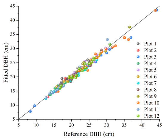
Figure 12.
Scatter plot of estimated DBH values.
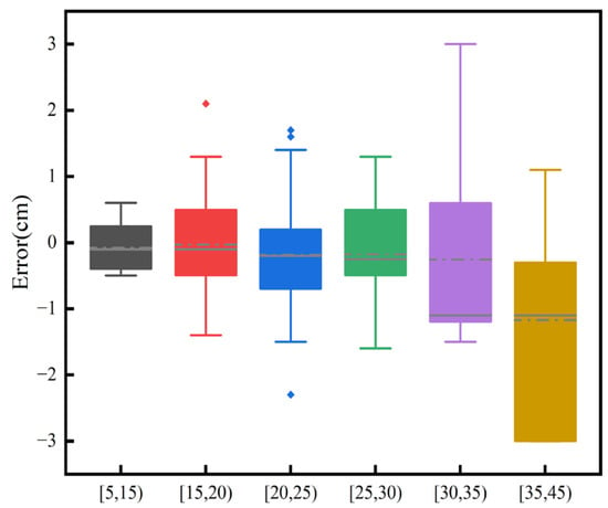
Figure 13.
The errors of DBH observations for different DBH values.
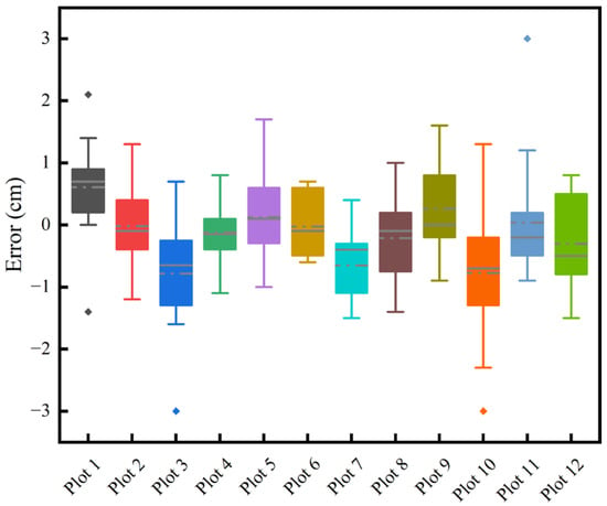
Figure 14.
The errors of DBH observations for different plots.
4.4.3. Estimating Tree Height
For tree height, BIAS ranged from −0.46 to 0.47 m, with relative bias varying between −3.97% and 1.87%, Table 4. The RMSE values fluctuated between 0.48 and 1.84 m, with the range of relative RMSE being 3.68% to 6.85%. As shown in Figure 15 and Figure 16, the dispersion of measurement errors and observed values gradually increases with the increase in tree height. Figure 17 shows that the error distribution between each plot’s measured and reference values is relatively uniform, and the distribution is random.

Table 4.
Accuracy of tree height estimations.
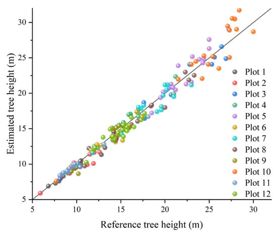
Figure 15.
Scatter plot of estimated tree heights.

Figure 16.
The errors in the tree height observations for different tree heights.

Figure 17.
The errors in the tree height observations for different plots.
5. Discussion
Monocular SLAM is one of the current mainstream systems, but no monocular SLAM solution exists for forest resource inventories. Therefore, this paper has developed a forest plot survey system that utilizes the array camera and IMU sensors provided by smartphones, as well as a data-processing platform based on a monocular SLAM system.
A portable RGB-D SLAM tree measurement system using SLAM technology has already been tested successfully [44], which is used to observe various parameters of individual trees in forests and to conduct forest plot surveys. Nowadays, the Google Tango platform that supports this system is no longer operational, and augmented reality technology projects like ARCore and ARKit have emerged as alternatives. Although these projects may have limitations in the precision of 3D data acquisition as a popular augmented reality technology, they do not require exceptional hardware support; they show significant advantages in device compatibility and popularity.
5.1. Tree Position Measurement
The tree position estimation was based on data obtained from device posture, which was also successfully tested by [44] with minimum error. Drift in device posture is a major factor affecting the accuracy of tree position. To overcome this problem, we performed loop closure detection and non-linear optimization of the pose graph, requiring the design of the measurement route to enable loop closure detection for repeated measurements [44].
The methodology depends on monocular SLAM in image recognition, automatically optimizing the position by recognizing set markers and passing them multiple times along the measurement path. Experimental results showed that the average error of this system in the x and y directions is about −0.11 to 0.16 m, with RMSEs of 0.05 to 0.18 m and 0.03 to 0.17 m, respectively. Similarly, [44] reports errors of about −0.12 to 0.13 m in the x- and y-axes, with RMSEs of 0.09 to 0.17 m and 0.07 to 0.17 m, respectively. In related research, the authors of [38] combined personal laser scanning (PLS) devices and SLAM technology to obtain the parameters of trees in forest plots, with the BIAS and RMSE of the position results being 0.24 m and 0.26 m, respectively, which is lower than the accuracy achieved in this research; furthermore, these studies were conducted in larger plots, so the system proposed in this study still needs to be tested in broader scenarios. In such scenarios, optimizing the position by passing markers multiple times could significantly extend the measurement time, leading to posture drift. For large plots, a more rational measurement path design and more marker settings may be required.
5.2. DBH Measurement
We attempted to attain the DBH values from point clouds. The method has been widely studied. Researchers also successfully extracted the DBH values of trees by finely fitting the columnar cloud and point cloud data obtained from TLS [49]. In single and multiple scans of TLS with the system BIAS, measurements ranged from −0.18 to 0.76 cm and 0.11 to 0.77 cm, respectively, while the RMSE fell between 0.74 to 2.41 cm and 0.9 to 1.9 cm. In another study [34], researchers used GNSS-IMU-assisted mobile laser scanning technology to estimate the DBH, reporting an average error of 0.63 cm, an RMSE of 3.06 cm, and a high determination coefficient (R2) of 0.97. Meanwhile, an innovative method of automatically estimating tree trunk diameters using a mobile ground laser scanner was performed by the authors of [31] and showed an average difference in DBH of 0.9 cm and a root mean squared error of 1.5 cm. In this study, the reported bias ranged from −0.78 to 0.61 cm, with RMSE values between 0.46 and 1.24 cm, similar to the results of laser radar measurements using high-precision point cloud data, possibly related to the application of AR technology. AR technology provides an intuitive means for observers to assess the accuracy of measurements.
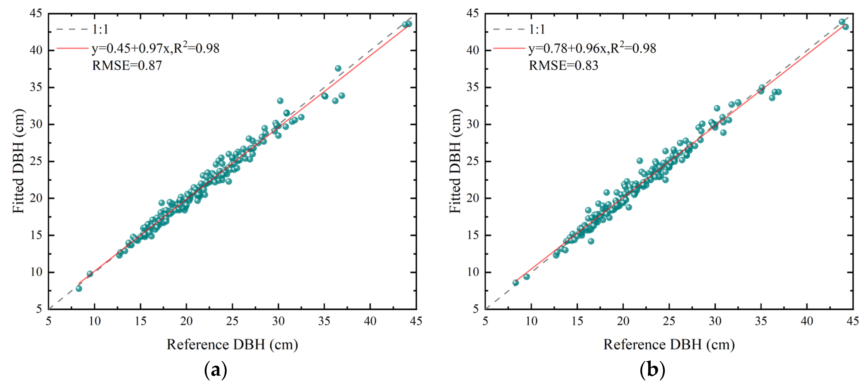
Furthermore, we also used an RGB-D SLAM tree measurement system with AR functionality [44] to measure the DBH of all the trees in 12 plots within the research area. We compared these results with the actual field measurements shown in Figure 18. Both systems had an R2 of 0.98, with RMSEs of 0.87 cm and 0.83 cm, respectively. This result indicates a high consistency in the measurement results of both methods and validates the hypothesis that AR technology can assist observers in intuitively assessing measurement accuracy.
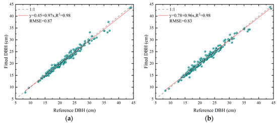
Figure 18.
Scatterplot of DBH measurements using a steel tape measure versus DBH measurements using other methods. (a) Scatterplot of DBH estimates from reference [44]; (b) scatterplot of DBH estimates in this paper.
As far as the technical application of the two systems is concerned, there are differences. The RGB-D SLAM tree measurement system can provide enough point clouds for circular fitting during scanning. In contrast, the system in this study relies on the tree surface having a sufficient texture to obtain the necessary point cloud density, requiring additional frame-filling measurements when the circular fitting is poor. Therefore, although the system in this study may not be as efficient as the RGB-D SLAM tree measurement system, the method of multi-angle frame filling for circular fitting can achieve better results when dealing with flat or irregularly shaped trees. The RGB-D SLAM system uses point clouds’ tangential and cutting point constraints in applying the DBH algorithm.
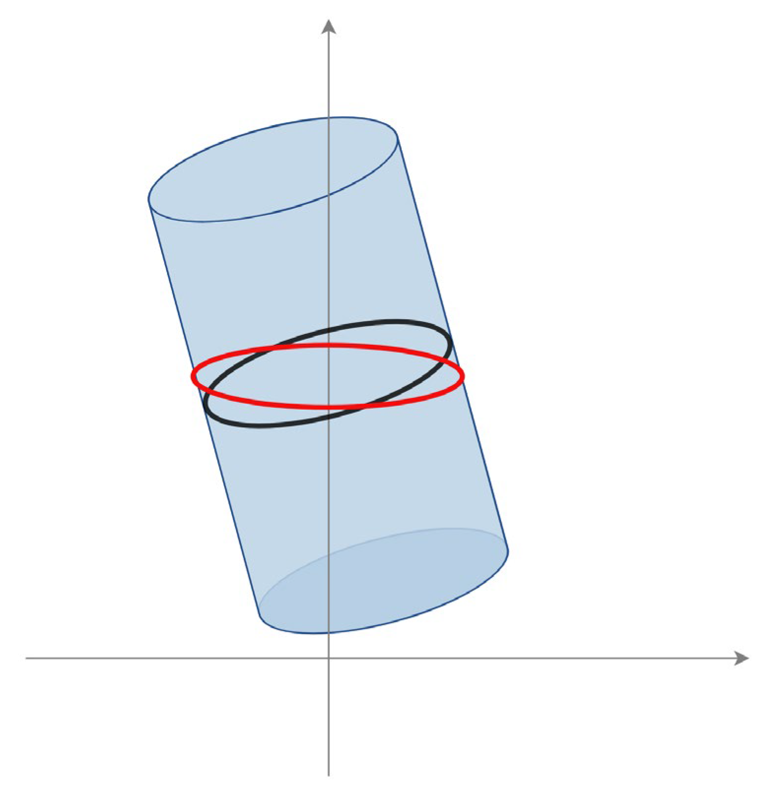
In contrast, this study uses cutting plane constraints to effectively solve the error caused by measuring inclined trees, as shown in Figure 19. RGB-D SLAM tree measurement systems and LiDAR point cloud DBH extraction usually use horizontal slices to extract point clouds for fitting, often fitting into the red circles shown in Figure 19, for measuring inclined trees, while cutting plane constraints can fit into the black circles. It is well known that an inclined cylinder’s slanted circumference is greater than its base’s circumference; therefore, algorithms without cutting plane constraints often lead to an overestimation of results. Figure 20 further shows the results of testing 30 inclined trees using the RGB-D SLAM tree measurement system (Figure 20A) and the system proposed in this paper (Figure 20B), showing that the RGB-D SLAM system generally leads to an overestimation when dealing with inclined trees. This problem is efficiently resolved in this paper.
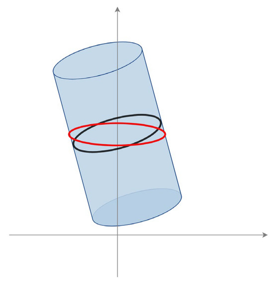
Figure 19.
Sources of error in measurement of DBH in inclined trees. The black circle is the correct-fit case. The red circle is the wrong-fit case.
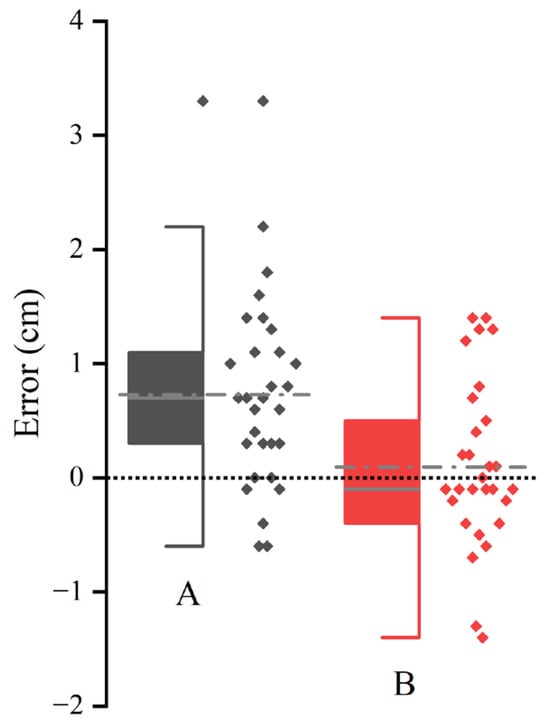
Figure 20.
Errors in observations of inclined trees by different methods. (A) is the method of reference [44]. (B) is the methodology of this paper.
5.3. Tree Height Measurement
This study has designed a novel method for measuring tree height by utilizing vector and plane relationships, and the use of augmented reality technology provides a visual interface for the real-time supervision of observations, thereby ensuring measurement accuracy. The experimental results show that the BIAS value of the measurements is approximately between −0.46 and 0.47 m, with an RMSE ranging from 0.48 to 1.84 m, with certain deviations in tree height estimation under different contexts. Still, overall, these errors are relatively small. As shown in Figure 16, the dispersion of measurement errors and observed values gradually increases with the increase in tree height. A clear trend is that, within the range of tree heights not exceeding 20 m, the measured values have more minor errors, but when the tree height exceeds 20 m, the measurement error significantly increases. Additionally, according to the data in Figure 17, it can be observed that in the Populus tomentosa plots 3, 5, and 10, the error is significantly increased compared to other plots, further emphasizing the increase in error when the tree height exceeds 20 m.
Research conducted by [14] and [17,18] evaluated the reliability and stability of tree height data obtained from airborne laser scanning (ALS), TLS, handheld personal laser scanning (PLShh), unmanned aerial vehicle laser scanning (ULS), and UAV photogrammetry (UAVimage) through field surveys. These devices reported average BIAS values for ALS, TLS, PLShh, ULS, and UAVimage of −0.12 m, −1.02 m, −0.45 m, −0.62 m, and −0.88 m, respectively; the average RMSE values were approximately 1.69 m, 2.11 m, 1.11 m, 1.38 m, and 1.58 m, respectively, unlike the above methods that measure tree height directly from point clouds. Still, smartphone cameras can only capture point cloud data within a limited distance range. The recommended threshold for reliable tree height measurement by TLS is below 25 m [8], which is higher than the optimal measurement range of the system in this paper.
In contrast, the methodology developed in this research shows more minor errors, which may be related to the supervisory effect provided by augmented reality. However, accurately displaying the top of the trees on a screen poses a challenge, particularly in forests with dense canopies. Users need to move to a position where they can observe the treetop [44], preferably at a horizontal distance from the tree similar to its height, to minimize the visual disparity effects induced by angles, which are more pronounced for taller trees. Meanwhile, with their aerial advantage, ALS, ULS, and UAVimage provide more reliable tree height data for taller trees, contrary to this study’s trend. On the other hand, PLShh shows a balanced performance across different tree height ranges, which this study has not achieved. Hence, future research must provide solutions for measuring taller trees and conduct extensive experimental validation. Other studies showed [44] that tree heights less than 20 m have a higher accuracy, with BIAS values approximately between −0.83 m and 2.08 m and RMSE values between 0.46 m and 2.44 m, consistent with the results of this study.
In SLAM algorithms, corners or blobs are typically chosen as visual feature points. Effective features should have a localized accuracy (both in position and scale), repeatability, and robustness, etc. However, identifying suitable corner points or blobs is challenging in forests with complex terrain and dense shrubs. Moreover, the presence of shrubs can obstruct the base marking of target trees, increasing the difficulty of localization. The plot data utilized in this study are sourced from human-accessible areas, where ground-level shrubs are relatively sparse. However, such terrain conditions are not representative of most forest environments, potentially posing greater challenges in practical applications.
The one limitation is that the current system can only measure trees one by one, which is less efficient, and there is still room for improvement in this system’s measurement methods. For example, marking at the base of the tree is currently required to assist in filtering point clouds for fitting the DBH. Still, this step is difficult to implement in dense shrubby vegetation. Also, when there is a bulge at the DBH position of the tree, it is impossible to deviate manually from the standard position for measurement, which not only reduces work efficiency but also affects the operational experience of forestry workers. Future system improvements must be able to fit diameters at any position, which will be more in line with humanized operation. Under the current technological environment, the lenses of most smartphones can only capture sparse point clouds through imaging, and the point cloud density is not rich. Devices with higher-performance lenses can provide dense point cloud data. Devices such as infrared-based RGB-D sensor devices [44] have a relatively low compatibility and popularity; with the continuous development of technology, it is believed that a balance can be found in these two aspects in the future. At the same time, research in forestry still needs to be deepened to promote technological progress and widespread application.
6. Conclusions
This paper provides a solution for the real-time estimation of inclined trees’ position, DBH, and height using monocular SLAM on a mobile phone when GNSS signals are unavailable. The paper utilizes cross-section constraint techniques and point cloud data for circular fitting to estimate the position and DBH of trees. The cross-section constraint method applies to situations where trees are inclined. Simultaneously, incorporating a multi-frame fitting approach effectively compensates for irregularities in tree trunks. The paper addresses the height measurement problem of inclined trees by utilizing real-time pose data provided by the SLAM system. The experimental results also showed that this method can accurately estimate the tree position, DBH, and height.
Using a monocular SLAM system and smartphones for forest plot surveys is feasible, and particularly suitable for forest areas with shorter trees. However, when dealing with taller trees, the system error significantly increases, so future research needs to improve further and optimize the system. At the same time, this equipment should be tested in more complex forest environments to enhance its robustness. Future research should also focus on extracting other forest attributes, such as stem curves, crown diameters, and tree trunk volume.
Author Contributions
Conceptualization, J.S.; methodology, J.S.; software, Y.F.; data processing, A.M.; formal analysis, Y.F.; data curation, J.S.; writing—original draft preparation, J.S.; writing—review and editing, L.L. and S.W.; supervision, Y.F.; project administration, Z.F.; funding acquisition, Z.F. All authors have read and agreed to the published version of the manuscript.
Funding
This study was supported by 5·5 Engineering Research & Innovation Team Project of Beijing Forestry University (BLRC2023A03) and the Natural Science Foundation of Beijing (8232038, 8234065), National Natural Science Foundation of China (42330507) and the Key Research and Development Projects of Ningxia Hui Autonomous Region (2023BEG02050).
Data Availability Statement
The data supporting the reported results are not publicly available due to privacy and ethical restrictions.
Acknowledgments
Special thanks to the editors and reviewers for their helpful comments and suggestions.
Conflicts of Interest
Author Lin Long was employed by the company China Construction Fifth Engineering Division Landscape Co., Ltd. The remaining authors declare that the research was conducted in the absence of any commercial or financial relationships that could be construed as potential conflicts of interest.
References
- Brodribb, T.J.; Powers, J.; Cochard, H.; Choat, B. Hanging by a Thread? Forests and Drought. Science 2020, 368, 261–266. [Google Scholar] [CrossRef]
- Gauthier, S.; Bernier, P.; Kuuluvainen, T.; Shvidenko, A.Z.; Schepaschenko, D.G. Boreal Forest Health and Global Change. Science 2015, 349, 819–822. [Google Scholar] [CrossRef]
- McDowell, N.G.; Allen, C.D.; Anderson-Teixeira, K.; Aukema, B.H.; Bond-Lamberty, B.; Chini, L.; Clark, J.S.; Dietze, M.; Grossiord, C.; Hanbury-Brown, A.; et al. Pervasive Shifts in Forest Dynamics in a Changing World. Science 2020, 368, eaaz9463. [Google Scholar] [CrossRef]
- Trumbore, S.; Brando, P.; Hartmann, H. Forest Health and Global Change. Science 2015, 349, 814–818. [Google Scholar] [CrossRef]
- Brolly, G.; Kiraly, G.; Lehtomaki, M.; Liang, X. Voxel-Based Automatic Tree Detection and Parameter Retrieval from Terrestrial Laser Scans for Plot-Wise Forest Inventory. Remote Sens. 2021, 13, 542. [Google Scholar] [CrossRef]
- Fan, Y.; Feng, Z.; Shen, C.; Khan, T.U.; Mannan, A.; Gao, X.; Chen, P.; Saeed, S. A Trunk-Based SLAM Backend for Smartphones with Online SLAM in Large-Scale Forest Inventories. ISPRS-J. Photogramm. Remote Sens. 2020, 162, 41–49. [Google Scholar] [CrossRef]
- Liang, X.; Hyyppa, J.; Kaartinen, H.; Lehtomaki, M.; Pyorala, J.; Pfeifer, N.; Holopainen, M.; Brolly, G.; Pirotti, F.; Hackenberg, J.; et al. International Benchmarking of Terrestrial Laser Scanning Approaches for Forest Inventories. ISPRS-J. Photogramm. Remote Sens. 2018, 144, 137–179. [Google Scholar] [CrossRef]
- Panagiotidis, D.; Abdollahnejad, A.; Slavík, M. 3D Point Cloud Fusion from UAV and TLS to Assess Temperate Managed Forest Structures. Int. J. Appl. Earth Obs. Geoinf. 2022, 112, 102917. [Google Scholar] [CrossRef]
- Surový, P.; Almeida Ribeiro, N.; Panagiotidis, D. Estimation of Positions and Heights from UAV-Sensed Imagery in Tree Plantations in Agrosilvopastoral Systems. Int. J. Remote Sens. 2018, 39, 4786–4800. [Google Scholar] [CrossRef]
- Balsi, M.; Esposito, S.; Fallavollita, P.; Nardinocchi, C. Single-Tree Detection in High-Density LiDAR Data from UAV-Based Survey. Eur. J. Remote Sens. 2018, 51, 679–692. [Google Scholar] [CrossRef]
- Cabo, C.; Ordonez, C.; Lopez-Sanchez, C.A.; Armesto, J. Automatic Dendrometry: Tree Detection, Tree Height and Diameter Estimation Using Terrestrial Laser Scanning. Int. J. Appl. Earth Obs. Geoinf. 2018, 69, 164–174. [Google Scholar] [CrossRef]
- Liang, X.; Kankare, V.; Yu, X.; Hyyppa, J.; Holopainen, M. Automated Stem Curve Measurement Using Terrestrial Laser Scanning. IEEE Trans. Geosci. Remote Sens. 2014, 52, 1739–1748. [Google Scholar] [CrossRef]
- Kuekenbrink, D.; Marty, M.; Boesch, R.; Ginzler, C. Benchmarking Laser Scanning and Terrestrial Photogrammetry to Extract Forest Inventory Parameters in a Complex Temperate Forest. Int. J. Appl. Earth Obs. Geoinf. 2022, 113, 102999. [Google Scholar] [CrossRef]
- Wang, Y.; Lehtomaki, M.; Liang, X.; Pyorala, J.; Kukko, A.; Jaakkola, A.; Liu, J.; Feng, Z.; Chen, R.; Hyyppa, J. Is Field-Measured Tree Height as Reliable as Believed A Comparison Study of Tree Height Estimates from Field Measurement, Airborne Laser Scanning and Terrestrial Laser Scanning in a Boreal Forest. ISPRS-J. Photogramm. Remote Sens. 2019, 147, 132–145. [Google Scholar] [CrossRef]
- Gollob, C.; Ritter, T.; Wassermann, C.; Nothdurft, A. Influence of Scanner Position and Plot Size on the Accuracy of Tree Detection and Diameter Estimation Using Terrestrial Laser Scanning on Forest Inventory Plots. Remote Sens. 2019, 11, 1602. [Google Scholar] [CrossRef]
- Liang, X.; Jaakkola, A.; Wang, Y.; Hyyppa, J.; Honkavaara, E.; Liu, J.; Kaartinen, H. The Use of a Hand-Held Camera for Individual Tree 3D Mapping in Forest Sample Plots. Remote Sens. 2014, 6, 6587–6603. [Google Scholar] [CrossRef]
- Jurjevic, L.; Liang, X.; Gasparovic, M.; Balenovic, I. Is Field-Measured Tree Height as Reliable as Believed—Part II, A Comparison Study of Tree Height Estimates from Conventional Field Measurement and Low-Cost Close-Range Remote Sensing in a Deciduous Forest. ISPRS-J. Photogramm. Remote Sens. 2020, 169, 227–241. [Google Scholar] [CrossRef]
- Gollob, C.; Ritter, T.; Nothdurft, A. Forest Inventory with Long Range and High-Speed Personal Laser Scanning (PLS) and Simultaneous Localization and Mapping (SLAM) Technology. Remote Sens. 2020, 12, 1509. [Google Scholar] [CrossRef]
- Liang, X.; Kankare, V.; Hyyppa, J.; Wang, Y.; Kukko, A.; Haggren, H.; Yu, X.; Kaartinen, H.; Jaakkola, A.; Guan, F.; et al. Terrestrial Laser Scanning in Forest Inventories. ISPRS-J. Photogramm. Remote Sens. 2016, 115, 63–77. [Google Scholar] [CrossRef]
- Wilkes, P.; Lau, A.; Disney, M.; Calders, K.; Burt, A.; de Tanago, J.G.; Bartholomeus, H.; Brede, B.; Herold, M. Data Acquisition Considerations for Terrestrial Laser Scanning of Forest Plots. Remote Sens. Environ. 2017, 196, 140–153. [Google Scholar] [CrossRef]
- Calders, K.; Adams, J.; Armston, J.; Bartholomeus, H.; Bauwens, S.; Bentley, L.P.; Chave, J.; Danson, F.M.; Demol, M.; Disney, M.; et al. Terrestrial Laser Scanning in Forest Ecology: Expanding the Horizon. Remote Sens. Environ. 2020, 251, 112102. [Google Scholar] [CrossRef]
- Chen, S.; Feng, Z.; Chen, P.; Khan, T.U.; Lian, Y. Nondestructive Estimation of the Above-Ground Biomass of Multiple Tree Species in Boreal Forests of China Using Terrestrial Laser Scanning. Forests 2019, 10, 936. [Google Scholar] [CrossRef]
- Raumonen, P.; Kaasalainen, M.; Akerblom, M.; Kaasalainen, S.; Kaartinen, H.; Vastaranta, M.; Holopainen, M.; Disney, M.; Lewis, P. Fast Automatic Precision Tree Models from Terrestrial Laser Scanner Data. Remote Sens. 2013, 5, 491–520. [Google Scholar] [CrossRef]
- Pitkanen, T.P.; Raumonen, P.; Kangas, A. Measuring Stem Diameters with TLS in Boreal Forests by Complementary Fitting Procedure. ISPRS-J. Photogramm. Remote Sens. 2019, 147, 294–306. [Google Scholar] [CrossRef]
- Balenovic, I.; Liang, X.; Jurjevic, L.; Hyyppa, J.; Seletkovic, A.; Kukko, A. Hand-Held Personal Laser Scanning—Current Status and Perspectives for Forest Inventory Application. Croat. J. For. Eng. 2021, 42, 165–183. [Google Scholar] [CrossRef]
- Cabo, C.; Del Pozo, S.; Rodriguez-Gonzalvez, P.; Ordonez, C.; Gonzalez-Aguilera, D. Comparing Terrestrial Laser Scanning (TLS) and Wearable Laser Scanning (WLS) for Individual Tree Modeling at Plot Level. Remote Sens. 2018, 10, 540. [Google Scholar] [CrossRef]
- Hyyppa, E.; Kukko, A.; Kaijaluoto, R.; White, J.C.; Wulder, M.A.; Pyorala, J.; Liang, X.; Yu, X.; Wang, Y.; Kaartinen, H.; et al. Accurate Derivation of Stem Curve and Volume Using Backpack Mobile Laser Scanning. ISPRS-J. Photogramm. Remote Sens. 2020, 161, 246–262. [Google Scholar] [CrossRef]
- Huncaga, M.; Chuda, J.; Tomastik, J.; Slamova, M.; Koren, M.; Chudy, F. The Comparison of Stem Curve Accuracy Determined from Point Clouds Acquired by Different Terrestrial Remote Sensing Methods. Remote Sens. 2020, 12, 2739. [Google Scholar] [CrossRef]
- Kuzelka, K.; Surovy, P. Mathematically Optimized Trajectory for Terrestrial Close-Range Photogrammetric 3D Reconstruction of Forest Stands. ISPRS-J. Photogramm. Remote Sens. 2021, 178, 259–281. [Google Scholar] [CrossRef]
- Mokros, M.; Mikita, T.; Singh, A.; Tomastik, J.; Chuda, J.; Wezyk, P.; Kuzelka, K.; Surovy, P.; Klimanek, M.; Zieba-Kulawik, K.; et al. Novel Low-Cost Mobile Mapping Systems for Forest Inventories as Terrestrial Laser Scanning Alternatives. Int. J. Appl. Earth Obs. Geoinf. 2021, 104, 102512. [Google Scholar] [CrossRef]
- Oveland, I.; Hauglin, M.; Gobakken, T.; Naesset, E.; Maalen-Johansen, I. Automatic Estimation of Tree Position and Stem Diameter Using a Moving Terrestrial Laser Scanner. Remote Sens. 2017, 9, 350. [Google Scholar] [CrossRef]
- Bauwens, S.; Bartholomeus, H.; Calders, K.; Lejeune, P. Forest Inventory with Terrestrial LiDAR: A Comparison of Static and Hand-Held Mobile Laser Scanning. Forests 2016, 7, 127. [Google Scholar] [CrossRef]
- Liang, X.; Kukko, A.; Hyyppa, J.; Lehtomaki, M.; Pyorala, J.; Yu, X.; Kaartinen, H.; Jaakkola, A.; Wang, Y. In-Situ Measurements from Mobile Platforms: An Emerging Approach to Address the Old Challenges Associated with Forest Inventories. ISPRS-J. Photogramm. Remote Sens. 2018, 143, 97–107. [Google Scholar] [CrossRef]
- Cernava, J.; Mokros, M.; Tucek, J.; Antal, M.; Slatkovska, Z. Processing Chain for Estimation of Tree Diameter from GNSS-IMU-Based Mobile Laser Scanning Data. Remote Sens. 2019, 11, 615. [Google Scholar] [CrossRef]
- Mur-Artal, R.; Montiel, J.M.M.; Tardos, J.D. ORB-SLAM: A Versatile and Accurate Monocular SLAM System. IEEE Trans. Robot. 2015, 31, 1147–1163. [Google Scholar] [CrossRef]
- Mur-Artal, R.; Tardos, J.D. ORB-SLAM2: An Open-Source SLAM System for Monocular, Stereo, and RGB-D Cameras. IEEE Trans. Robot. 2017, 33, 1255–1262. [Google Scholar] [CrossRef]
- Kukko, A.; Kaijaluoto, R.; Kaartinen, H.; Lehtola, V.V.; Jaakkola, A.; Hyyppa, J. Graph SLAM Correction for Single Scanner MLS Forest Data under Boreal Forest Canopy. ISPRS-J. Photogramm. Remote Sens. 2017, 132, 199–209. [Google Scholar] [CrossRef]
- Chen, S.; Liu, H.; Feng, Z.; Shen, C.; Chen, P. Applicability of Personal Laser Scanning in Forestry Inventory. PLoS ONE 2019, 14, e0211392. [Google Scholar] [CrossRef]
- Hyyppa, E.; Hyyppa, J.; Hakala, T.; Kukko, A.; Wulder, M.A.; White, J.C.; Pyorala, J.; Yu, X.; Wang, Y.; Virtanen, J.-P.; et al. Under-Canopy UAV Laser Scanning for Accurate Forest Field Measurements. ISPRS-J. Photogramm. Remote Sens. 2020, 164, 41–60. [Google Scholar] [CrossRef]
- Fan, Y.; Feng, Z.; Yan, F.; Shen, C.; Guan, T.; Su, J. Design and Experiment of Monocular SLAM Augmented Reality Tree Measurement System. Trans. Chin. Soc. Agric. Mach. 2023, 54, 259–266. [Google Scholar]
- Hyyppa, J.; Virtanen, J.-P.; Jaakkola, A.; Yu, X.; Hyyppa, H.; Liang, X. Feasibility of Google Tango and Kinect for Crowdsourcing Forestry Information. Forests 2018, 9, 6. [Google Scholar] [CrossRef]
- Gollob, C.; Ritter, T.; Krassnitzer, R.; Tockner, A.; Nothdurft, A. Measurement of Forest Inventory Parameters with Apple iPad Pro and Integrated LiDAR Technology. Remote Sens. 2021, 13, 3129. [Google Scholar] [CrossRef]
- Tomastik, J.; Salon, S.; Tunak, D.; Chudy, F.; Kardos, M. Tango in Forests—An Initial Experience of the Use of the New Google Technology in Connection with Forest Inventory Tasks. Comput. Electron. Agric. 2017, 141, 109–117. [Google Scholar] [CrossRef]
- Fan, Y.; Feng, Z.; Mannan, A.; Khan, T.U.; Shen, C.; Saeed, S. Estimating Tree Position, Diameter at Breast Height, and Tree Height in Real-Time Using a Mobile Phone with RGB-D SLAM. Remote Sens. 2018, 10, 1845. [Google Scholar] [CrossRef]
- Fan, Y. Research on Key Technologies of Portable RGB-D SLAM Tree Measurement System. Ph.D. Thesis, Beijing Forestry University, Beijing, China, 2021. [Google Scholar]
- Qin, T.; Li, P.; Shen, S. VINS-Mono: A Robust and Versatile Monocular Visual-Inertial State Estimator. IEEE Trans. Robot. 2018, 34, 1004–1020. [Google Scholar] [CrossRef]
- Goesele, M.; Snavely, N.; Curless, B.; Hoppe, H.; Seitz, S.M. Multi-View Stereo for Community Photo Collections. In Proceedings of the IEEE 11th International Conference on Computer Vision, Rio de Janeiro, Brazil, 14–21 October 2007; IEEE: New York, NY, USA, 2007; pp. 1–8. [Google Scholar]
- Merrell, P.; Akbarzadeh, A.; Wang, L.; Mordohai, P.; Frahm, J.-M.; Yang, R.; Nister, D.; Pollefeys, M. Real-Time Visibility-Based Fusion of Depth Maps. In Proceedings of the IEEE 11th International Conference on Computer Vision, Rio de Janeiro, Brazil, 14–21 October 2007; IEEE: New York, NY, USA; pp. 1–8. [Google Scholar]
- Liang, X.; Hyyppa, J. Automatic Stem Mapping by Merging Several Terrestrial Laser Scans at the Feature and Decision Levels. Sensors 2013, 13, 1614–1634. [Google Scholar] [CrossRef] [PubMed]
Disclaimer/Publisher’s Note: The statements, opinions and data contained in all publications are solely those of the individual author(s) and contributor(s) and not of MDPI and/or the editor(s). MDPI and/or the editor(s) disclaim responsibility for any injury to people or property resulting from any ideas, methods, instructions or products referred to in the content. |
© 2024 by the authors. Licensee MDPI, Basel, Switzerland. This article is an open access article distributed under the terms and conditions of the Creative Commons Attribution (CC BY) license (https://creativecommons.org/licenses/by/4.0/).


