Abstract
Forest canopy image is a necessary technical means to obtain canopy parameters, whereas image segmentation is an essential factor that affects the accurate extraction of canopy parameters. To address the limitations of forest canopy image mis-segmentation due to its complex structure, this study proposes a forest canopy image segmentation method based on the parameter evolutionary barnacle optimization algorithm (PEBMO). The PEBMO algorithm utilizes an extensive range of nonlinear incremental penis coefficients better to balance the exploration and exploitation process of the algorithm, dynamically decreasing reproduction coefficients instead of the Hardy-Weinberg law coefficients to improve the exploitation ability; the parent generation of barnacle particles ( = 0.5) is subjected to the Chebyshev chaotic perturbation to avoid the algorithm from falling into premature maturity. Four types of canopy images were used as segmentation objects. Kapur entropy is the fitness function, and the PEBMO algorithm selects the optimal value threshold. The segmentation performance of each algorithm is comprehensively evaluated by the fitness value, standard deviation, structural similarity index value, peak signal-to-noise ratio value, and feature similarity index value. The PEBMO algorithm outperforms the comparison algorithm by , and for each evaluation metric, respectively. The experimental results show that the PEBMO algorithm can effectively improve the segmentation accuracy and quality of forest canopy images.
1. Introduction
Image segmentation is the process of dividing the pixel points of the original image into different categories of sub-regions according to attributes such as color, texture, and intensity value, and then completing the process of extracting the target in the image [1]. Standard segmentation methods include the thresholding method [2,3,4,5], region technique [6], watershed algorithm [7], and deep learning [8,9,10]. The region-based segmentation method has a severe segmentation deficiency for aggregated particle adhesion [11]. The watershed algorithm has the disadvantage of over-segmentation and reflected light interfering with the image [12]. Deep learning is widely used in forest canopy image segmentation owing to its high segmentation accuracy, robustness, adaptability, and ability to handle large-scale data. U-Net, Mask R-CNN and Transformers are classical segmentation modules in deep learning. However, segmentation methods based on deep learning also suffer from high training cost. They are long and time-consuming, have limitations in being sensitive to noise, and are not suitable for segmenting small-sample images with little feature information and high randomness. Compared to the deep learning method, the threshold segmentation method utilizes the information in the image histogram to find the threshold value of the image. It distinguishes different target and background regions by setting multiple threshold values [13]. Since it relies on simple mathematical operations, it outperforms complex deep learning models in terms of processing speed. The key to threshold segmentation is selecting an appropriate segmentation method to determine the segmentation threshold. Threshold selection methods based on information entropy have attracted considerable attention owing to their clear mathematical concepts. Otsu entropy [14], Renyi entropy [15], and Kapur entropy [16] are typical information entropy methods. The Otsu method selects segmentation thresholds to maximize the variance between the target and background classes. It is suitable for the case where the area occupied by the target and the background in the image are close, and the Otsu segmentation method will be invalid when the area occupied by the two is disparate [17]. The essence of Renyi entropy is to use the subordination function to convert the image histogram information into a fuzzy domain and then obtain the optimal threshold value to segment the image based on the principle of maximum entropy [18]. The adjustable parameter is an essential parameter in Renyi entropy, and the value of determines the form of Renyi entropy. Although different segmentation effects can be obtained by adjusting , it is a challenge to select the optimal parameter reasonably. Improper selection may lead to over-segmentation or under-segmentation phenomenon. The segmentation principle of Kapur entropy is that the total entropy value of the target class and the background class is the maximum. Because Kapur entropy is based on the grey level intra-class probability when calculating the entropy value, it is not sensitive to the size of the divided target and background, can better retain small targets in the image [19], and is widely used in color image segmentation.
Forest canopy images have various complex backgrounds, and the gray levels vary widely, requiring multiple thresholds for accurate segmentation. Traditional image segmentation methods use enumeration, and when performing threshold segmentation, each combination must be individually tested to select the optimal threshold. The computational complexity increases exponentially with an increase in the number of thresholds. To overcome these limitations, scholars view finding the optimal thresholds in multithreshold segmentation as an optimization problem with constraints. Heuristic optimization algorithms search for optimal thresholds to reduce the computational complexity. Intelligent optimization algorithms, such as the Golden Jackal Optimization Algorithm [20], Elephant Herding Optimization Algorithm [21], Sand Cat Optimization Algorithm [22], and Dung Beetle Optimization Algorithm [23] have been successfully applied to image segmentation. Studies have shown that the performance of intelligent algorithms significantly affects the segmentation accuracy and efficiency of the images. Therefore, improving intelligent algorithms to enhance their performance and image segmentation accuracy and efficiency has become the focus of research. Sukanta Nama proposes a quasi-reflected slime mold (QRSMA) method combined with a quasi-reflective learning mechanism. The results of the CEC2020 benchmark function tests showed that QRSMA outperformed the statistical, convergence, and diversity measures of the slime mold algorithm. It also outperformed other existing methods for segmenting COVID-19 X-ray images [24]. Jiquan Wang et al. proposed a Whale Optimization Algorithm combining mutation and de-similarity to address the limitations of the whale optimization Algorithm easily falling into local optimal solutions. Multilevel threshold segmentation was performed on ten grayscale images using Kapur and Otsu as the objective function. The experimental results showed that CRWOA outperformed the five compared algorithms in terms of convergence and segmentation quality [25]. Essam H. Houssein et al. proposed a chimpanzee optimization algorithm (IChOA) based on the strategy of contrastive learning and Levy Flight improvement. IChOA was tested on a dataset from the database of infrared images using Otsu and Kapur methods. The experimental results show that the IChOA is robust for segmenting various positive and negative cases [26]. Laith Abualigah et al. proposed a novel hybrid algorithm (MPASSA) to determine the optimal thresholds in multi-threshold segmentation by borrowing the properties of the Marine Predator and Salp Swarm Algorithm. Multiple benchmark images were used to verify the performance of the MPASSA. The experimental results show that MPASSA avoids the problem of falling into the local optima. It also has a strong solution capability for image-segmentation problems [27].
To address the problems of poor segmentation accuracy of forest canopy images due to complex structure and uneven illumination, Wu et al. proposed a segmentation method based on differential evolutionary whale optimization algorithm [28]; Tong et al. proposed a segmentation method based on improved northern goshawk algorithm by using multi-strategy fusion [29]; Wang et al. proposed a segmentation method based on improved tuna swarm optimization [30]. The experimental results show that compared with the original algorithm, the improved algorithm obtains higher segmentation accuracy in segmenting forest canopy images. It proves the effectiveness and necessity of the improved intelligent algorithm in multi-threshold segmentation of forest canopy images. In recent years, scholars have been enthusiastic about innovative algorithms, and many intelligent algorithms with excellent performance have appeared, bringing new vitality to the research on image multi-threshold segmentation. The BMO is a novel bionic evolutionary optimization algorithm proposed by Sulaiman et al. (2018) that simulates the mating behavior of barnacles in nature to solve the optimization problem [31]. Since its proposal, it has received extensive attention from scholars. In [32], quasi-inverse dyadic learning and logistic chaotic mapping were used to solve the problem of the premature convergence of the BMO algorithm. Literature [33] used random wandering was used to replace the random logarithm in the remote insemination iteration formula. The parameter p was replaced with a logistic chaotic mapping operator to improve the problem of premature convergence of the BMO algorithm. Literature [34] improved the penis coefficient and the remote insemination iterative formula using a logistic model to achieve adaptive transformation of parameters as well as to avoid falling into local optima. In [35], cubic chaos initialization was used to improve the diversity of the initial population, the parameter p was replaced with a hyperbolic sinusoidal modulation factor to improve the convergence speed of the algorithm, and Gaussian and Cosey variants were introduced to solve the shortcomings of the BMO, which is prone to fall into local optimother. The literature [36] integrates barnacle larvae settlement and adhesion behavior to increase population diversity and improve the global exploration performance of the algorithm. It also uses positive and negative decline casting strategies to improve the local mining ability.
The BMO algorithm exhibited an excellent performance and fewer control parameters. However, these parameters have a more significant impact on the performance of the BMO algorithm. Many improvements have also focused on the importance of the parameters of the BMO algorithm, and the direction of its improvement is almost always centered around the parameters. This is explicitly embodied in the following aspects: (1) The fixed penis coefficient makes the exploration and exploitation process unbalanced, although the literature [34] realized the adaptive conversion of , the range of variation of was small, and there was not much difference with the fixed penis coefficient. (2) The Hardy-Weinberg law coefficient p plays a decisive role in the exploitation ability of the BMO algorithm, and fixed coefficients cannot maintain the diversity of the populations, which weakens the exploitation ability of the BMO algorithm. Literature [33] utilized Logistic Chaos coefficients instead of the parameter p. Although Logistic Chaos coefficients have strong ergodicity, their iteration sequences are unevenly distributed, which is not conducive to increasing population diversity. Reference [35] designed a nonlinearly decreasing parameter p in the interval , which aims to accelerate the convergence speed of the algorithm, but p tends to 0 in the late iteration, which also results in the loss of population diversity. In addition, to improve the ability of the BMO algorithm to jump out of the local optimal solution, ref. [35] added a double perturbation, which effectively enhances the ability of the algorithm to jump out of the local optimal solution but also slows down the convergence speed of the algorithm.
This paper proposes a PEBMO algorithm and applies it to the multi-threshold segmentation of forest canopy images. Specifically, the main contributions of this study are (a) to address the limitations of the BMO algorithm, a wide range of nonlinear increasing penis coefficients, dynamically decreasing reproduction coefficients, and Chebyshev chaotic perturbation strategies are employed to improve the balance between exploration and exploitation, the exploitation ability, and the resistance to premature maturation of the BMO algorithm; (b) the PEBMO algorithm is combined with Kapur entropy to determine the optimal segmentation threshold to improve the segmentation efficiency and accuracy of forest canopy images; and (c) to investigate the performance of PEBMO and PEBMO-based segmentation methods on the 2017 test function and forest canopy image problems, respectively. (d) We compared PEBMO with five BMO variant algorithms. PEBMO performed better than the other BMO-variant algorithms. The forest canopy image segmentation results show that PEBMO-based segmentation methods outperform the artificial bee colony optimization algorithm (ABC) [37], chimp optimization algorithm (ChOA) [38], cuckoo algorithm (CS) [39], flower pollination algorithm (FPA) [40], mayfly algorithm (MA) [41], improved mayfly algorithm (IMA) [42], and BMO.
2. Materials and Methods
2.1. Materials
The canopy images used in the experiment were obtained from the Liangshui Experimental Forestry Farm of Northeast Forestry University. They were acquired randomly by a Panasonic DMC-LX5 camera (Panasonic Company, Kadoma City, Osaka, Japan) fisheye lens Samyang AE 8/3.5 Aspherical IF MC Fisheye (Samyang Optics, Changwon, Gyeongsangnam-do, Republic of Korea). The Liangshui Experimental Forest Farm is located in the southern section of the Xiaoxinganling Mountain Range (eastern slope of the Dali Belt Range branch) in the eastern mountains of northeast China. The geographic coordinates are 128°–128° E, 47°–47° N. This location is on the eastern edge of the Eurasia continent, which is deeply influenced by the oceanic climate and has prominent temperate continental monsoon climate characteristics. In winter, under the control of the metamorphic continental air masses, the climate is cold, dry, and windy. In summer, under the influence of subtropical metamorphic oceanic air masses, precipitation is concentrated (of which June–August accounts for more than 60% of annual precipitation), and temperature is high. The climate in spring and fall is variable and spring is windy, with little precipitation, and prone to drought. In the fall, the temperature drops sharply, and early frosts occur more often. The soils in the region are divided into four soil classes (drenching soil class, Semi-hydro pedogenic class, pedogenic class, and organic soil class), four soil classes (dark brown loam, meadow soil, swamp soil, and peat soil), and 14 subclasses. Because the altitude of this area is not high, there is no apparent high mountain, and the vertical distribution of soil is not apparent, only a territorial distribution pattern. Red pine, spruce forests and birch forests dominate in the forest field, accounting for 63.7%, 11.4% and 6.4% of the forested area respectively. The forest cover rate is 98%.
2.2. Basic BMO
Initialization: In the BMO algorithm, barnacles are candidate solutions and the following matrix represents their population vectors:
N is the number of control variables (problem dimensions) and n is the population size or the number of barnacles. The upper-and lower-bound constraints for each control variable are as follows:
where and denote the upper and lower bounds of the ith variable, respectively. First, the initial population X is evaluated, then the fitness value of each barnacle is ranked, and the barnacle with the best current fitness value is ranked at the top of X.
Selection: Randomly selecting the father and mother to be mated from the barnacle population, the formulae for selection are shown in (4) and (5):
where denotes the father to be mated and denotes the mother to be mated.
Reproduction: The value is essential to determine the exploration and exploitation processes. The value in the basic BMO algorithm is set to 7. If , the barnacle algorithm reproduces the offspring according to the Hardy-Weinberg theorem, which is the exploitation phase of the BMO algorithm. The barnacle mating iteration formula is given by (6).
where p and q are the percentages of characteristics of the father and mother in the next generation, respectively. Where p is a random number uniformly distributed in and , and are the variables of father and mother selected by Equations (4) and (5), respectively.
If , the offspring are produced by remote insemination, and this process can be considered as an exploration phase with the iterative formula shown in (7):
where is a random number within , which can be seen from Equation (7) that the mother determines the generation of offspring during remote insemination.
2.3. PEBMO
2.3.1. Large Range of Non-Linear Increasing Penis Coefficients
The penis coefficient directly determines the transition between the exploration and exploitation of BMO algorithms. In the basic BMO algorithm, is fixed value 7. A fixed penis coefficient defeats the original purpose of the metaheuristic algorithm of dynamic balance between exploration and exploitation. Therefore, it is necessary to design a dynamic adaptive penis coefficient to improve the flexibility between exploration and exploitation. The improved parameter is given by Equation (8).
where t is the current number of iterations, and T is the maximum number of iterations.
As can be seen from Equation (8), consists of three parts: is the range adjustment part that determines the overall range of . was initially designed to utilize the nonlinearity of to enhance the balance between algorithm exploration and exploitation, and the nonlinearity of the exponential function meets this requirement. The designed increases nonlinearly in the interval [7, 26.95], which makes the value smaller at the beginning of the iteration and gradually increases at the end of the iteration. determines the overall trend of and is the core part of . However, gradually reached its maximum value at the end of the iteration and remained there until the end. The that no more changes increases the probability of the algorithm falling into a locally optimal solution. Therefore, it is necessary to make change slightly at the end to enhance the diversity of the population. However, a significant increase is detrimental to the fast convergence of the algorithm. Therefore, a nonlinearly increasing in the interval [0, 1.5506] compensates for these shortcomings.
A parameter ranging in the interval [7, 28] and increasing nonlinearly with the number of iterations was designed. At the beginning of the iteration, the value was small, and most of the barnacle particles were outside the range of the value to fully explore the solution space. As the number of iterations increased, the value increased nonlinearly, and the algorithm gradually transitioned from the exploration phase to the exploitation phase. At the end of the iteration, the value reached approximately 28, at which time most particles were in the exploitation stage. However, a small number of barnacle particles still perform global exploration to find possible global optimal solutions. This design not only makes the exploration and exploitation process of the BMO algorithm well balanced and speeds up the algorithm’s convergence but also increases the adaptivity of the algorithm. The proposed optimization mechanism is illustrated in Figure 1.

Figure 1.
optimization mechanism.
2.3.2. Dynamically Decreasing Reproduction Factor
In the exploitation phase, the parameter p significantly affects the exploitation capability of the BMO algorithm. In the basic BMO algorithm, p is a fixed value of 0.6 for each iteration, and the fixed parameter decreases the diversity of offspring propagated by Equation (6), resulting in a weak local exploitation capability of the algorithm and a slow convergence rate.
The dynamic decreasing coefficients in the white-crowned chicken optimization algorithm [43] provide a faster convergence rate and stronger exploitation capability. Inspired by the white-crowned chicken optimization algorithm, this study uses the dynamic parameter instead of p in the exploitation phase of the white-crowned chicken optimization algorithm. The iterative formula is as follows:
where t is the number of current iterations; T is the maximum number of iterations; is a random number in [−1, 1]; and R is a random number in the interval (0, 1). It can be seen from Figure 2a that fluctuates uniformly in the interval (−1, 1). The introduction of increases the variability of . From Figure 2b, the value of decreases gradually from the (−2, 2) interval to the (−1, 1) interval. Even at the end of the iteration, fluctuates in the (−1, 1) interval, which fully retains the diversity of the population and improves the exploitation ability of the algorithm. decreases linearly with the number of iterations in the (1, 2) interval, and it can be seen from the comparison of Figure 2a,b that the addition of not only improves the range of fluctuation of but also accelerates the convergence speed of the algorithm. The improved iteration formula is as follows:
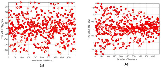
Figure 2.
Change curve of and , (a) is the change curve of , (b) is the change curve of .
2.3.3. Optimal Neighbourhood Chebyshev Chaotic Perturbations
When the algorithm is stalled, there are two cases: (1) the algorithm finds the global optimal solution, and the search for the optimal solution is complete; (2) the algorithm is stuck in the local optimal solution. It is not sufficiently comprehensive to perturb the algorithm solely because it stagnates. Some scholars add perturbation at the optimal solution, which increases the population diversity near the optimal solution and prevents the algorithm from maturing prematurely at the optimal solution; however, it also affects the convergence speed. Therefore, in this study, we added Chebyshev chaotic perturbation to the mother generation of barnacle particles at . The iterative formula of Chebyshev chaotic mapping is shown below:
where k is the order.
When , the perturbation equation is as follows:
Figure 3 shows ten common chaotic mappings. The figure shows that the Chebyshev chaotic perturbation has good randomness with a perturbation range of [−1, 1], which is more significant than other chaotic perturbations and produces a wider global distribution of particles with more comprehensive information. Adding the perturbation at = 0.5 can maximize the retention of possible optimal solutions in the late iteration and increase the algorithm’s ability to jump out of the local optimal solution.
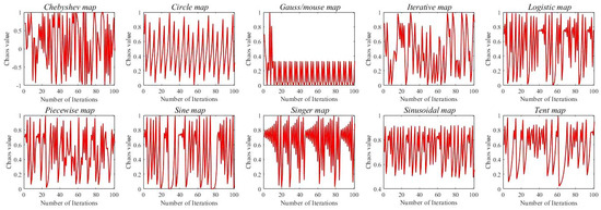
Figure 3.
Common 10 chaotic mappings.
2.3.4. Convergence Rate Analysis
The PEBMO algorithm is designed to achieve improved performance by improving the algorithm parameters. The large range of nonlinear increasing penis coefficients, dynamic decreasing reproduction coefficients, and optimal neighborhood Chebyshev chaotic perturbations all have some effect on the convergence speed. It is analyzed explicitly as follows:
In intelligent algorithm optimization, the balance between exploration and exploitation has a significant impact on the convergence speed of the algorithm. If the algorithm is too biased towards exploration (global search), it may waste a lot of time in irrelevant regions, resulting in slow convergence. If the algorithm is too biased toward exploitation (local search), it may fall into the local optimal solution prematurely and fail to find the global optimum. The is a parameter that regulates the balance between the exploration and exploitation of the BMO algorithm, and it is a fixed value 7. A fixed search range may result in the algorithm not being able to cover the global space at the initial stage or not being able to optimize it at a later stage. Therefore, in this study, a large range of non-linear increasing penis coefficients is designed to better balance the BMO algorithm exploration and exploitation process. At the beginning of the iteration, the value is large, and the vast majority of barnacle particles are in the exploration stage to explore the solution space. As the number of iterations increases, the value decreases, and most of the particles are in the exploration stage, finely exploiting the searched region. The large range of non-linear increasing penis coefficients enables the algorithm to find the best trade-off between global search and local optimization, thus finding the optimal solution more efficiently and significantly accelerating the convergence speed.
The parameter p of the BMO algorithm in the exploitation phase directly determines the behavior of the algorithm in the local search and optimization process. If the exploitation intensity is too great, it may lead to a decrease in population diversity, and the algorithm falls into a local optimum; if the exploitation intensity is too low, it cannot fully utilize the regional information, and the convergence speed is slow. In the BMO algorithm, p is a random number between (0, 1). Although the random number can increase the population diversity in the exploitation phase, over-reliance on random exploration will lead to unclear search direction and slow convergence. The dynamic decreasing reproduction coefficient varies in a large range in the early period of iteration, giving the algorithm a strong ability to fully exploit the explored region in search of a possible optimal solution. As the number of iterations increases, the range of p decreases, avoiding over-exploitation and speeding up convergence. The design of the dynamically decreasing reproduction coefficient better balances the exploitation intensity and thus accelerates the convergence rate.
In order to improve the ability of the algorithm to jump out of the local optimal solution, adding perturbations to the optimal solution to increase the diversity of the population is an effective strategy for improvement. However, it also brings the defect of slow convergence speed of the algorithm. Therefore, in this study, the ability of the algorithm to jump out of the local optimal solution is increased by adding the Chebyshev chaotic perturbation at = 0.5. The limitation of excessive perturbation at the optimal solution, which leads to non-convergence of the algorithm, is avoided.
2.4. PEBMO Algorithm Design
In this study, the exploration and exploitation process of the BMO algorithm is made more homogeneous by the design of a large range of penis coefficients; the introduction of the dynamic decreasing reproduction coefficients increases the diversity of the populations and improves the exploitation capability of the algorithm; and the Chebyshev chaotic perturbation at = 0.5 increases the ability of the algorithm to jump out of the local optimal solution. The flowchart of PEBMO is shown in Figure 4.

Figure 4.
Flowchart of PEBMO algorithm.
The basic steps of the PEBMO algorithm are as follows:
1. Randomly generate an initial population with a population size of N. Initialize the position of each barnacle particle using Equation (1) and set the parameters required for the execution of the algorithm: N, n, T, .
2. Calculate the fitness value of each barnacle particle and rank them, The optimal solution at the top ( = the current optimal solution).
3. Calculate value according to Equation (8); Calculate value according to Equation (12); Calculate value according to Equation (14).
4. Select dad according to Equation (4) and Mum according to Equation (5).
5. If the penis length of the chosen father is less than , the offspring are generated according to Equation (13); otherwise, the offspring are generated according to Equation (7).
6. If the penis length of the selected parent is 0.5, offspring are generated according to Equation (15).
7. The fitness value of each barnacle particle is calculated.
8. Sorting and update .
9. Determine whether the iteration termination condition is met; if so, exit the loop; otherwise, proceed to Step 2.
2.5. Forest Canopy Image Segmentation Based on the PEBMO Algorithm
2.5.1. Multi-Level Threshold Image Segmentation
Threshold segmentation can be classified into second-and multilevel thresholds according to the number of thresholds [44]. Second-level segmentation divides an image into two parts, target and background, by a single threshold and is suitable for segmenting simple images. Multilevel threshold segmentation divides an image into regions with different gray levels using various thresholds, which is ideal for segmenting complex multi-target images. Canopy images contain more information and single-threshold segmentation is insufficient to complete the segmentation task. For multilevel threshold segmentation, suppose n thresholds are , and the grey level mapping is
where is gray level of the segmented image; . Equation (16) shows that the key step of threshold segmentation is to select the optimal threshold related to the segmentation quality. Kapur entropy was used as the objective function in this study.
2.5.2. Kapur Entropy
Kapur entropy is a more commonly used information-entropy-based threshold selection method that is widely used in the multi-threshold segmentation of complex images. The principle of multi-threshold image segmentation based on Kapur entropy is as follows:
Assuming that the image gray level is L and the gray range is , the probability of a pixel in this gray level can be expressed as
where represents the sum of the number of pixels with gray level i and N represents the total number of pixels in the image. The Kapur entropy objective function for multi-thresholding is defined as:
Among them,
is the entropy of different categories after segmentation, is the probability of pixel points occurrence in each category, and is the probability of pixel points with grey value j.
A judgment is made according to Equation (23) to select the optimal combination of thresholds.
The maximized combination is the optimal threshold sought to solve the problem of the best combination of thresholds. Therefore, using an intelligent optimization algorithm to select the optimal threshold can effectively solve the problems of low efficiency and accuracy of traditional methods. In this study, PEBMO was used to select an optimal threshold.
2.5.3. Implementation of the PEBMO-Based Segmentation Algorithm
In order to improve the segmentation performance of the canopy image, Kapur entropy is the fitness function, and the PEBMO algorithm searches for the optimal threshold to segment the canopy image accurately. Figrue Figure 5 shows the flowchart of the proposed multi-threshold segmentation of the canopy image based on the PEBMO algorithm. The framework of the proposed algorithm is as follows:
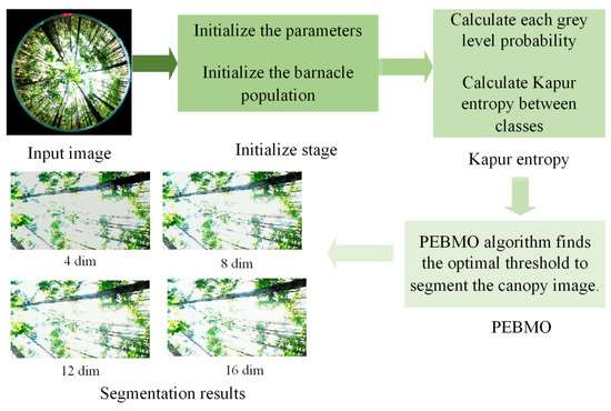
Figure 5.
Multi-level threshold segmentation framework based on PEBMO algorithm.
1. Input the image to be segmented.
2. Generate the population and parameters of PEBMO.
3. Calculate each grey level’s probability (22).
4. Calculate the fitness value of each search agent by using (19) for Kapur entropy.
5. PEBMO algorithm finds the optimal threshold to segment the canopy image.
6. Output the segmentation result.
3. Results
This section consists of two parts: the testing and validation of the PEBMO algorithm’s performance and the testing and validation of the PEBMO-based segmentation algorithm.
3.1. Performance Testing and Analysis of the PEBMO Algorithm
3.1.1. CEC2017 Test Functions
CEC2017 is a collection of test functions used in the 2017 IEEE Congress on Evolutionary Computation (CEC) competition, and the essential information is shown in Table 1. Among them, are single-peak functions containing only one global optimal solution, which are used to test the convergence speed and local search ability of the algorithm. shows unstable behavior, especially for higher dimensions, and significant performance variations for the same algorithm implemented. For high-dimensional test functions, is usually excluded. Since this study is not a high-dimensional testing study, however, is also tested. are multi-peak functions containing multiple local optimal solutions, which are used to test the exploration ability of the algorithms and the ability to jump out of the local optimal solutions. Such functions are adapted to test the performance of algorithms in solving complex multipeak optimization problems. are hybrid functions that contain multiple functions combined to create variety and complexity. are composite functions, which are combinations of various simple functions, each of which is univariate but combined to form a high-dimensional composite function. Hybrid and composite functions were used to solve large-scale optimization problems and test the potential of the algorithms to solve complex problems in the real world.

Table 1.
Basic information about CEC2017 test functions. * shows unstable behavior, especially for higher dimensions, and significant performance variations for the same algorithm implemented. For high-dimensional test functions, is usually excluded. Since this study is not a high-dimensional testing study, however, is also tested.
3.1.2. Experimental Setup
The experiment was conducted on a Dell Computer USA. The model number is the Alienware G15 5530 1526. It is configured for an Intel CPU @2.50 GHz, 16 GB of RAM, and a Windows 11 operating system. This equipment was purchased from Suihua, China. The PEBMO algorithm was compared with five BMO variants to verify its performance. The algorithm parameters are listed in Table 2. The population size of the experiment was set to 30, and the maximum number of iterations was 500. Each benchmark function was independently run 30 times to avoid chance errors in the optimization search. The fitness value, standard deviation, and convergence curve were used as evaluation indexes. The best results are shown in bold font.
Table 2.
Parameter setting for each algorithm.
3.1.3. Sensitivity Analysis
In order to objectively analyze the influence of the changes of parameters N and T on the accuracy and stability of the PEBMO algorithm’s optimization search, a sensitivity analysis is carried out. Table 1 is used as the test function, and the average adaptability and standard deviation values are the evaluation indices. The average fitness values reflect the optimization accuracy of the algorithm. The standard deviation reflects the stability of an algorithm. The optimization accuracy and stability of the PEBMO algorithm are verified at different N and T values, respectively. Figure 6a shows the number of the optimal average fitness values and standard deviation values obtained by the PEBMO algorithm at different values of N. The figure shows that the PEBMO algorithm obtains 13, 10, 6, and 4 optimal average fitness values and 11, 10, 3, and 6 optimal standard deviation values when N is 30, 40, 50, and 60, respectively. No optimal fitness values and standard deviation values were obtained for N of 5, 10 and 20. This is due to the fact that the algorithm cannot fully explore the solution space when N is small, and the computational complexity increases when N is large. Therefore, neither too large nor too small N is conducive to the algorithm’s optimization search. It is worth noting that there are three sets of juxtaposed optimal values in obtaining the average fitness value, thus leading to more than 30 total optimal averages. Figure 6b shows the number of the optimal average fitness values and standard deviation values obtained by the PEBMO algorithm at different values of T. From the figure, it can be seen that the effect on the average fitness values is more significant at different T values compared to the standard deviation values. Thirteen optimal average fitness values and eight optimal standard deviation values were obtained at T = 500, which are better than the other T values.
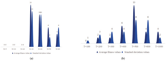
Figure 6.
Histogram of the distribution of optimal values in the parameter sensitivity test. (a) Histogram of the distribution of the optimal average fitness values and standard deviation values for different values of N; (b) is a histogram of the distribution of optimal average fitness values and standard deviation values for different values of T.
To summarize, the parameters N and T affect the evaluation of the algorithm’s performance. Too large and too small N and T are not conducive to the algorithm performance test. The experimental results show that the PEBMO algorithm obtains the most optimal fitness values and standard deviation values when N = 30, which is 43.33% and 36.67% better than other particle numbers, respectively. As for the number of iterations, the PEBMO algorithm obtained 43.33% of the optimal average fitness value and 26.67% of the optimal standard deviation value when T = 500, which is better than other T values. Therefore, in the algorithm performance testing experiments, the number of population particles is N = 30, and the number of iterations is chosen as T = 500.
3.1.4. Analysis of Optimization Accuracy and Stability Score
Figure 7 and Figure 8 show the histograms of the distribution of the optimal mean fitness and number of standard deviation values for each BMO variant algorithm on the CEC2017 test function, respectively. The average fitness value reflects the optimization accuracy of the algorithm and the standard deviation value reflects its stability.
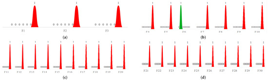
Figure 7.
Histogram of the distribution of the optimal average fitness values obtained by each BMO variant algorithm on the cec2017 test function. Where yellow is literature [32], green is literature [33], light blue is literature [34], blue is literature [35], purple is literature [36], black is BMO, and red is PEBMO. (a) is a histogram of the single-peak function; (b) is a histogram of the multi-peak function; (c) is a histogram of the hybrid function; (d) is a histogram of the composite function.
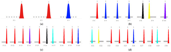
Figure 8.
Histogram of the distribution of the optimal standard deviation values obtained by each BMO variant algorithm on the cec2017 test function. Where yellow is literature [32], green is literature [33], light blue is literature [34], blue is literature [35], purple is literature [36], black is BMO, and red is PEBMO. (a) is a histogram of the single-peak function; (b) is a histogram of the multi-peak function; (c) is a histogram of the hybrid function; (d) is a histogram of the composite function.
Figure 7 and Figure 8 show that, in comparison with the BMO variant algorithm, the PEBMO algorithm performs well in terms of seeking accuracy, better than the BMO variant algorithm, and better than the base BMO algorithm. This shows that the PEBMO algorithm has a high optimization accuracy and that the improvement of the PEBMO algorithm by each strategy is effective. PEBMO algorithm outperformed the comparison algorithm by in optimization accuracy on the single-peak function and stability. This is owing to the introduction of the dynamically decreasing reproduction coefficient p, which effectively improves the exploitation capability of the BMO algorithm. IBMO [33] and IBMO [35] also improved parameter p to improve its exploitation capability. As can be seen from the test results in Table 3, the improvement effect is average and not as good as that of the other BMO variants of the algorithm.
Table 3.
Parameter setting for deep learning.
The PEBMO algorithm has a more substantial optimization accuracy on the multipeak function, better than the comparison algorithm, indicating that the PEBMO algorithm has a strong global optimization ability and the ability to jump out of the local optimal solution. The BMO algorithm also performs well on the multipeak function, indicating that the BMO algorithm itself has good global optimization ability. To improve the global optimality-seeking ability of the BMO algorithm, IBMO [34] replaced ( ) with the chaos vector obtained from the logistic chaos mapping, and IBMO [36] added coefficients to ( ). The test results in Table 3 show that for the optimization of the multi-peak function, the optimization accuracy of IBMO [34] and IBMO [36] is not as good as that of the BMO algorithm, which is why this study does not improve the exploration phase of the BMO algorithm. The PEBMO algorithm outperforms the BMO algorithm because the extensive range of incremental penis coefficients, , provides a better balance between the exploration and exploitation of the BMO algorithm.
Chebyshev chaos perturbation at allows the algorithm to jump out of the local optimal. Chebyshev chaotic perturbation, although it provides the PEBMO algorithm with a higher accuracy in finding the optimal on the multi-peak function, it also leads to less stability than IBMO [35]. IBMO [35] obtained optimal standard deviation values for , and , but their average fitness values were poor. This shows that the algorithm fails to effectively jump out of the local optimal solution for these three functions and falls into a precocious situation. In addition, IMBO [35] has a large stability gap for different functions and achieves optimal standard deviation values for , and . At the same time, it is almost the worst value for other functions, especially , and , which is inferior to other algorithms. This phenomenon also proves that the instability effect caused by the double disturbance was significant. However, whether the perturbation of IMBO [35] is strong or weak, its optimization search accuracy is not as good as that of the other algorithm variants.
The PEBMO algorithm has a significant advantage in hybrid and composite functions and is better than the comparison algorithms in terms of optimization accuracy. It is better than the comparison algorithm in terms of stability, and better than the BMO algorithm. This shows that the PEBMO algorithm is more comprehensive and has a high optimization accuracy and stability in optimizing large-scale and realistic problems, with obvious advantages.
3.1.5. Statistical Analysis
The Wilcoxon rank–sum test is a nonparametric statistical method for comparing differences between two independent groups of samples. Compared to the t-distribution test, Fisher’s exact test, and Kruskal–Wallis H test, it has the advantage of not requiring the assumption that the data obeys a specific probability distribution, is stable and unaffected by outliers, and is simple, convenient, intuitive, and easy to understand. Therefore, it is widely used to evaluate the differences between the performance of each algorithm. Where 0.05 is the significance level, a p-value greater than 0.05 indicates that the difference between the two groups is not significant, and a p-value less than 0.05 indicates that the difference between the two groups is significant. The Wilcoxon–rand rank sum test values for each algorithm are shown in Figure 9. Where the black horizontal line is the significance level value of 0.05, from the figure, it can be seen that the p-values obtained by the PEBMO algorithm in the determination of the differences with the other algorithms are less than 0.05, which indicates that the PEBMO algorithm has been significantly improved. In addition, there is no distribution of values on some functions (e.g., –), which is because the p-value obtained on this function is too small, much less than 0.05; therefore, it is not significantly represented in the graph.
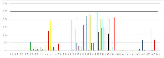
Figure 9.
The Wilcoxon–rand rank sum test values for each algorithm. Among them, PEBMO vs. IBMO [32] is yellow, PEBMO vs. IBMO [33] is green, PEBMO vs. IBMO [34] is blue, PEBMO vs. IBMO [35] is purple, PEBMO vs. IBMO [36] is black, and PEBMO vs. BMO is red.
3.1.6. Convergence Analysis
The convergence curve of the function can intuitively reflect the convergence speed, accuracy, and ability of each algorithm to jump out of the local optimal solution. Figure 10 shows the convergence curve of some functions, in which the horizontal axis indicates the number of iterations and the vertical axis indicates the value of the optimal fitness.
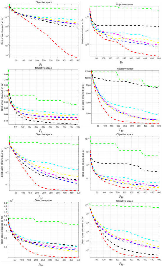
Figure 10.
Convergence curves of the BMO algorithm and the BMO variant algorithm (dark blue for ABMO [29]; black for IBMO [30]; yellow for IBMO [31]; green for IBMO [32]; light blue for IBMO [33]; violet for BMO; and red for PEBMO. the designation value of is 100; the designation value of is 200; The designation value of is 600; the designation value of is 1000; the designation value of is 1200; the designation value of is 1800; the designation value of is 2600; the designation value of is 3000).
On the convergence curve of the single-peak function, it can be seen that the red PEBMO curve has apparent fluctuations in the middle and late iteration, indicating that even in the late iteration, the diversity of the population is not lost and still has a strong exploitation ability. On the convergence curve of the multi-peak function , the fitness value of the PEBMO algorithm is not as good as that of IBMO [30], which is consistent with the data in Table 3. For , the convergence curve of the PEBMO algorithm is at the bottom of all curves, indicating that its fitness value is better than that of the comparison algorithm. The PEBMO curve was located at the bottom of the hybrid and composite function convergence curves. It converges slowly in the late iteration, indicating that the PEBMO algorithm has high optimization accuracy and good stability.
3.2. Experimental Results and Analysis of Canopy Segmentation
3.2.1. Data Analyses
The forest canopy is intricate and complex, and the canopy images obtained by the fisheye lens often have quality problems, such as uneven illumination and loss of details. They also often have the limitation of low segmentation accuracy when segmenting the canopy images. Therefore, before segmenting the canopy image, this paper uses the literature [45] method to enhance different canopy images. The enhanced canopy images are shown in Figure 11, Figure 12, Figure 13 and Figure 14. Figure 11 shows two different types of nonuniform canopy images. Among them, the overall brightness of the LS1–LS3 images was low, and only a small part was in the exposure state. By contrast, the brightness of the LB1–LB3 images was not as high as that of LS1–LS3. However, the bright area is large; therefore, accurately segmenting the boundaries of the bright regions is an excellent test for the segmentation algorithm. Figure 12 shows the canopy images acquired under low-illumination conditions. The tone is dark, especially at low tree trunks, and it is easily misclassified as background. Figure 13 shows a canopy image acquired under strong sunlight, where intense sunlight blurs the treetops bordering the sky because of the sun’s reflection, and it is very easy to misclassify faint foliage as the sky. Figure 14 shows a canopy image acquired under normal lighting conditions. However, because of the acquisition method (elevation shot) and the forest gap, there was low brightness and unclear details at the low tree trunks, even under ideal lighting conditions.
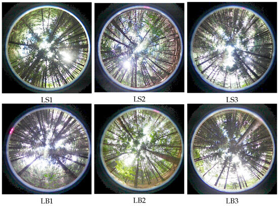
Figure 11.
Non-uniform canopy images processed by reference [45]. (LS1, LS2 and LS3 are small-area exposure images; LB1, LB2, and LB3 are large-area exposure images).

Figure 12.
Low-light canopy images processed by reference [45]. (L1 and L4 are local high-light canopy images; L2 is a canopy image with uneven canopy distribution; L3 is a canopy image with uniform canopy distribution).
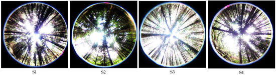
Figure 13.
Strong illuminated canopy image processed by literature [45]. (S1 has slight colour distortion; S2 image has low contrast; S3 has colour degradation; S4 image has low saturation).

Figure 14.
Normal illumination canopy images processed by literature [45]. (N1–N4 are images obtained at different periods. Where, N1: 08:00, N2: 10:00, N3: 12:00 and N4: 14:00).
3.2.2. Experimental Setup
In this section, segmentation experiments are conducted on Figure 11, Figure 12, Figure 13 and Figure 14 to evaluate the effectiveness of the proposed PEBMO algorithm on the multi-threshold segmentation of forest canopy images. The population size (N) was set to 30, maximum number of iterations was 500, and number of thresholds (dim) was set to , and 16. To verify the effectiveness of PEBMO in the multithreshold segmentation of forest canopy images. The segmentation results of the PEBMO algorithm were compared with those of ABC, ChOA, CS, FPA, MA, IMA, and BMO. structural similarity index (SSIM), peak signal-to-noise ratio (PSNR), feature similarity index (FSIM), and subjective evaluation metrics were used to assess the quality of the segmentation results.
3.2.3. Image Evaluation Metrics
SSIM considers the characteristics of the human visual system by measuring the similarity between the original and segmented images in terms of brightness, contrast, and structural similarity [46]. The SSIM value is located in the interval [0, 1], and the larger its value, the more similar is the segmented image to the original image. The formula for calculating SSIM is as follows:
where and denote the mean and variance of the original image, respectively; and denote the mean and variance of the segmented image; and is the covariance between the original image and the segmented image; and and are constants. , .
PSNR is the ratio of an image’s maximum possible pixel value to the minimum pixel difference caused by noise in the image [47]. Its magnitude directly depends on the intensity of the image. The larger the PSNR value, the more significant the noise-removal effect and the lower the image distortion [48]. The PSNR value was calculated as follows:
and are the original and segmented images, respectively, and H and W are the image dimensions.
FSIM is another method for assessing the feature similarity after SSIM [49]. Unlike SSIM, it measures image quality by evaluating the feature similarity between the original and segmented images. The better the image quality, the closer the value is to 1. The formula for the FSIM is shown in Equation (30).
where is the pixel value of the entire image, denotes the similarity value, and represents the phase consistency measure.
and denote the phase coherence of the reference and segmented images, respectively.
where denotes the feature similarity of the image; denotes the gradient similarity of the image; and represent the gradient magnitude of the reference image and the segmented image, respectively; and are constants.
3.2.4. Image Segmentation Accuracy Analysis
The line graph of the fitness value obtained by each algorithm is shown in Figure 15. The fitness value effectively reflects the segmentation accuracy of the image. The larger its value, the higher the segmentation accuracy. From the figure, it can be seen that the fitness value fold is approximated as a triangular wave, indicating that the segmentation accuracy of each algorithm increases with the increase in the number of thresholds. When the number of thresholds is 4, the adaptation value of each algorithm is low, and the difference is not significant, indicating that none of the algorithms can segment the image accurately. As the number of thresholds increases, the gap between the algorithms is gradually apparent. The PEBMO algorithm has a clear advantage and is located at the top, indicating that its segmentation accuracy is better than the comparison algorithms. As shown in Table A8 in Appendix A, the improved algorithms IMA and PEBMO obtain 22 and 29 optimal adaptation values, respectively, accounting for , while MA obtains the other two optimal values. In addition, compared with the essential MA and BMO algorithms, IMA and PEBMO improved and in segmentation accuracy, respectively. It shows that the improvement of algorithm performance can effectively improve the segmentation accuracy of canopy images. In the comparison between IMA and PEBMO, the PEBMO algorithm is better than IMA, indicating that the segmentation accuracy of the PEBMO algorithm is better than the IMA algorithm.
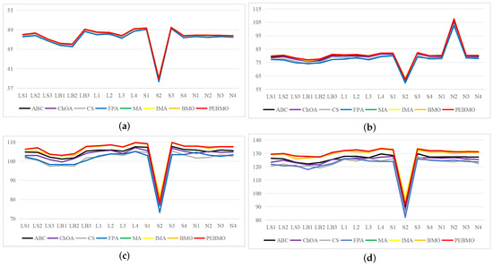
Figure 15.
Line graph of optimal fitness values obtained by each algorithm (where (a) is the line graph of fitness values for a threshold number of 4, (b) is the line graph of fitness values for a threshold number of 8, (c) is the line graph of fitness values for a threshold number of 12, and (d) is the line graph of fitness values for a threshold number of 16).
3.2.5. Image Segmentation Stability Analysis
The line graph of the standard deviation values obtained by each algorithm is shown in Figure 16. The standard deviation values reflect the stability of the algorithms. The lower its value, the higher the stability. As can be seen from the graph, the PEBMO algorithm has apparent advantages, except for the noticeable fluctuation in the S4 image with eight thresholds. It is located at the lowest end on all other images, which indicates that it has strong stability in segmenting the canopy image. As can be seen from Table A9, PEBMO obtains 55.56% of the optimal standard deviation value. This is due to the effective improvement in the performance of the PEBMO algorithm, which enables the PEBMO algorithm to segment all types of canopy images accurately. IMA, which is also an improved algorithm, however, only obtained 23.61% of the optimal values but outperformed MA by 79.17%, indicating the effectiveness of the improvement of the IMA algorithm as well. The ABC, ChOA, CS, FPA, MA and BMO algorithms, on the other hand, performed mediocrely, with optimal values of 1, 1, 2, 3, and 3, respectively.
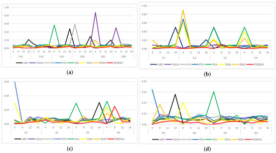
Figure 16.
Line graph of standard deviation values obtained by each algorithm (where (a) is the line graph of standard deviation values for non-uniform canopy images, (b) line graph of standard deviation values for low illumination canopy images, (c): line graph of standard deviation values for strongly illuminated canopy images, and (d): line graph of standard deviation values for normally illuminated canopy images).
3.2.6. Structural Similarity Analysis
The line graph of SSIM values obtained by each algorithm is shown in Figure 17. The SSIM value reflects the structural similarity between the segmented image and the original image. The larger its value, the better the quality of the segmented image. As the number of thresholds increases, the SSIM value increases, but the stability of the algorithms is poor on the N2 image. The FPA, MA, IMA, BMO and PEBMO algorithms all show higher SSIM values for low thresholds than for high thresholds, and this is due to the fact that the branches and leaves in the N2 image are intricate and more difficult to segment, which is more challenging for the algorithms. Therefore, an unstable fluctuation phenomenon occurs during segmentation. ABC, ChOA, and CS algorithms do not show any fluctuation. Still, their SSIM values are lower, which indicates that ABC, ChOA and CS fall into local optimal solutions in segmentation and fail to segment the image accurately. Overall, IMA and PEBMO algorithms have apparent advantages. As shown in Table A10, the IMA and PEBMO algorithms obtain 63.89% of the optimal SSIM values. The advantages of IMA are concentrated on S1–S4 and N1–N4. The PEBMO algorithm outperforms the comparison algorithm on LS1–LS3, LB1–LB3, and L1–L4 images, whereas it is significantly inferior to IMA on S1–S4 and N1–N4 images. This indicates that the PEMBO algorithm is not as good as the IMA algorithm in segmenting strong and normal light canopy images.
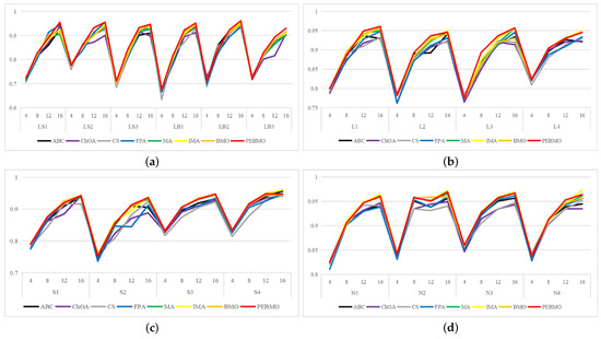
Figure 17.
Line graph of SSIM values obtained by each algorithm (where (a) is the line graph of standard deviation values for non-uniform canopy images, (b) line graph of standard deviation values for low illumination canopy images, (c): line graph of standard deviation values for strongly illuminated canopy images, and (d): line graph of standard deviation values for normally illuminated canopy images).
3.2.7. Analysis of Image Distortion Level
The line graph of PSNR values obtained by each algorithm is shown in Figure 18. The PSNR values reflect the degree of distortion of the segmented image. From the graph, it can be seen that the IMA and PEBMO algorithms have a clear advantage and are located at the top of the image, indicating that their segmented canopy images are less distorted and of better quality. The excellent performance of the IMA and PEBMO algorithms is due to the effective improvement of the MA and BMO algorithms. On the L1–L4 images, the segmentation stability of the algorithms is high, and there is no apparent fluctuation. In addition, as shown in Table A11, the IMA and PEBMO algorithms improved 72.22% and 76.39% in segmentation quality relative to the original algorithms, respectively. IMA only obtained three optimal values, although 75% better than the MA algorithm, which indicates that IMA is not good at segmenting non-uniform canopy images.
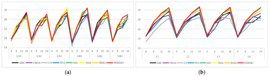
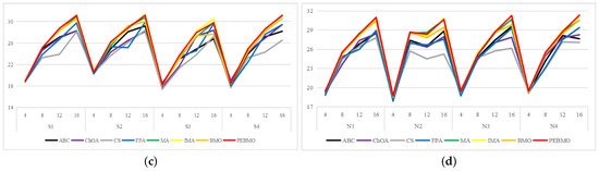
Figure 18.
Line graph of PSNR values obtained by each algorithm (where (a) is the line graph of standard deviation values for non-uniform canopy images, (b) line graph of standard deviation values for low illumination canopy images, (c): line graph of standard deviation values for strongly illuminated canopy images, and (d): line graph of standard deviation values for normally illuminated canopy images).
3.2.8. Feature Similarity Analysis
The line graph of FSIM values obtained by each algorithm is shown in Figure 19. From the figure, it is clear that the algorithms have obtained high FSIM values on all the images. Among them, it is higher than 0.83 on LS1–LB3 images, 0.94 on L1–L4 images, 0.93 on S1–S4 images, and 0.95 on L1–L4 images. This stems from the fact that the original image prior to segmentation has a better quality, and hence, enhancement before segmentation is necessary. As the number of thresholds increases, the FSIM value also increases. The advantage of the PEBMO algorithm is obvious: almost all of them are located in the topmost part of the image, which indicates that its segmented image is more similar to the original image in terms of structure and better quality. In addition, as shown in Table A12, the optimal FSIM values are mainly distributed in MA, BMO, IMA and PEBMO algorithms, accounting for 81.94%. Among them, MA, BMO, IMA and PEBMO obtained 9.72%, 15.28%, 30.56% and 33.33% of the optimal values, while ABC, ChOA, CS and FPA obtained 6.94%, 2.78%, 2.78% and 5.56% of the optimal values, respectively.
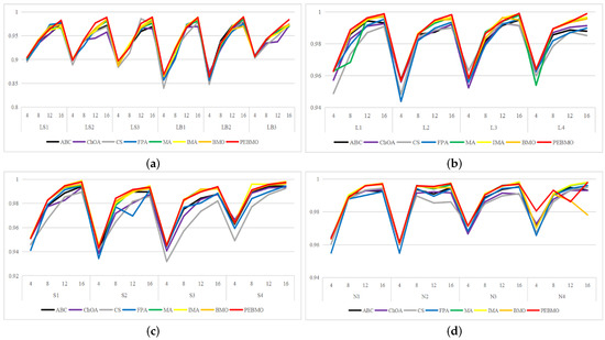
Figure 19.
Line graph of FSIM values obtained by each algorithm (where (a) is the line graph of standard deviation values for non-uniform canopy images, (b) line graph of standard deviation values for low illumination canopy images, (c): line graph of standard deviation values for strongly illuminated canopy images, and (d): line graph of standard deviation values for normally illuminated canopy images).
3.2.9. Segmentation Efficiency Analysis
The computation time for each algorithm for various types of canopy images is shown in Figure 20, Figure 21, Figure 22 and Figure 23. Computation time reflects the segmentation efficiency of each algorithm. Overall, the magnitude of the computation time for each algorithm is . The computation time of the PEBMO algorithm is located at a medium level and inferior to that of BMO, which stems from the fact that to increase the probability of the BMO algorithm jumping out of the locally optimal solution, the parent generation of barnacle particles of = 0.5 is subjected to the Chaos Perturbation of Chebyshev. The introduction of this link undoubtedly increased the running time of the PEBMO algorithm. However, the difference between the computational method times of the PEBMO and BMO algorithms was not significant. In addition, the time required by all the algorithms to increase from four dimensions to 16 dimensions is not more than 5 s, which also proves that the introduction of intelligent algorithms can effectively improve the limitations of the inefficiency of the multithreshold segmentation method.
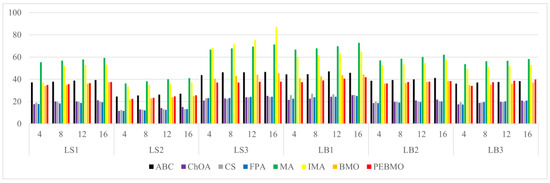
Figure 20.
Histogram of segmentation time for each algorithm on non-uniformly illuminated canopy images.
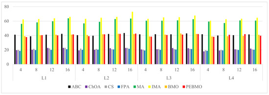
Figure 21.
Histogram of segmentation time for each algorithm on low illumination canopy image.
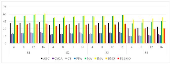
Figure 22.
Histogram of segmentation time for each algorithm on strongly illuminated canopy images.
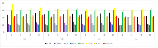
Figure 23.
Histogram of segmentation time for each algorithm on normal illumination canopy image.
3.3. Comparison of PEBMO and Deep Learning
3.3.1. Hyperparametric Analysis
In order to evaluate the PEBMO algorithm objectively and comprehensively, the segmentation results of the PEBMO algorithm are comprehensively compared with the deep learning segmentation method in terms of fitness values, standard deviation values, SSIM, PSNR, FSIM, and computation time. A Transformer segmentation module was used for deep learning. To analyze the effect of different hyperparameters (num_layers and ) on the model performance. Hyperparameter analysis experiments were designed. Figure 24 shows the distribution of adaptation values, PSNR, SSIM, FSIM, computation time and standard deviation values for different and num_layers conditions. The analysis and summary of Figure 24 is shown below:
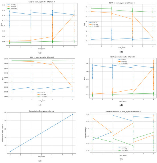
Figure 24.
The distribution of each evaluation metric for different and num_layers. (where (a): the distribution of Loss values for different and num_layers, (b): the distribution of PSNR values for different and num_layers, (c): the distribution of SSIM values for different and num_layers, (d): the distribution of FSIM values for different and num_layers, (e): the distribution of average computation time for different and num_layers, (f): the distribution of standard deviation values for different and num_layers).
(1) Effect of num_layers and learning rate () on the Loss function
With the increase of num_layers, the Loss value shows an overall increasing trend. When num_layers = 2, the Loss is lower; while num_layers = 8, the Loss is higher. Increasing the number of layers may lead to overfitting of the model, especially when the amount of data is limited. A smaller learning rate ( = 0.0001) usually leads to lower Loss values.
(2) Effect of num_layers and on PSNR
The value of PSNR is higher when num_layers = 2; it decreases as the number of layers increases. When num_layers = 2, the average PSNR value is greater than 62 for = 0.0001; it decreases for num_layers = 8. Smaller learning rates ( = 0.0001) usually result in higher PSNR values. It is clearly seen that the FSNR values for = 0.0001 are generally higher than the FSNR values for = 0.01 and 0.001.
(3) Effect of num_layers and on SSIM
Similar to PSNR, SSIM is higher for num_layers = 2; it gradually decreases as the number of layers increases, and the value of SSIM is generally higher when the learning rate = 0.0001.
(4) Effect of num_layers and on FSIM
In contrast to PSNR and SSIM, FSIM is lower for num_layers = 2; it gradually increases as the number of layers increases, and the value of SSIM is generally higher when the learning rate = 0.01.
(5) Effect of num_layers and lr on computation time
The learning rate has a negligible impact on the computation time, and the average computation time is mainly affected by num_layers; the more num_layer layers there are, the longer the computation time will be.
(6) Standard deviation analysis
The standard deviation of Loss: A smaller (e.g., = 0.0001) usually results in a lower standard deviation, indicating more stable model training.
When num_layers is increased, the model may be overfitted, leading to an increase in Loss and a decrease in PSNR and SSIM. A smaller learning rate (e.g., = 0.0001) usually leads to better performance and more stable training. Therefore, to ensure better time and model performance, this study uses the parameter combination num_layers = 4, = 0.0001.
3.3.2. Analysis of Comparative Results
The relevant settings are listed in Table 3. The obtained segmentation results are shown in Figure 25, Figure 26, Figure 27, Figure 28 and Figure 29, respectively. It is worth noting that the gap between the deep learning method and the PEBMO algorithm is large in all the evaluation metrics; therefore, Figure 25, Figure 26, Figure 27, Figure 28 and Figure 29 are all double vertical axis bar charts. The left side is the vertical axis of the PEBMO algorithm and the right side is the vertical axis of deep learning.
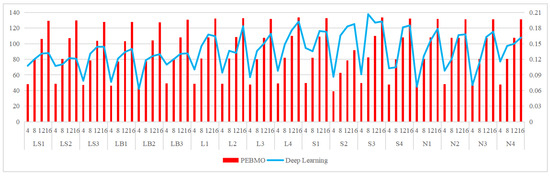
Figure 25.
Schematic comparison between the PEBMO algorithm and deep learning algorithm in terms of fitness value.
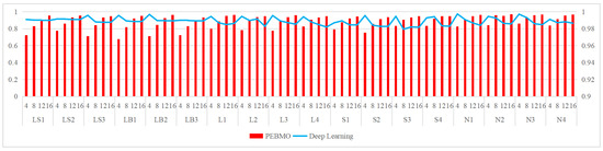
Figure 26.
Schematic comparison between the PEBMO algorithm and deep learning algorithm in terms of SSIM value.
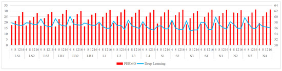
Figure 27.
Schematic comparison between the PEBMO algorithm and deep learning algorithm in terms of PSNR value.
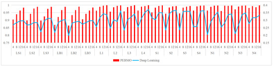
Figure 28.
Schematic comparison between the PEBMO algorithm and deep learning algorithm in terms of FSIM value.
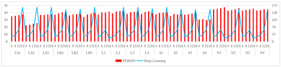
Figure 29.
Schematic comparison of the PEBMO algorithm and deep learning algorithm in terms of computation time.
As can be seen from the data in the table, there are significant differences between the deep learning segmentation algorithm and the PEBMO segmentation algorithm in several performance metrics. The advantages and disadvantages of deep learning and PEBMO algorithms are as follows:
1. Advantages of Deep Learning
(a) Deep learning segmentation methods generally have higher SSIM and PSNR values than the PEBMO algorithm at all thresholds. This indicates that deep learning algorithms are better able to capture the structural and feature information of an image, thereby providing higher-quality segmentation results.
(b) Deep learning is highly adaptable, can handle complex scene data, and has strong generalization ability. This makes it more advantageous for complex image segmentation tasks.
2. The shortcomings of Deep learning:
(a) It is less stable and susceptible to parameters that prevent it from maintaining consistent performance with different inputs.
(b) Although it outperforms the PEBMO algorithm in terms of computation time for individual images, it takes longer to compute at high thresholds and requires high-performance hardware support. This may limit their use in real-time applications.
(c) The data dependency is strong and requires a large amount of labelled data for training, which requires high data quality. If the data is insufficient or inaccurately labelled, the segmentation accuracy may be affected.
3. Advantages of the PEBMO algorithm:
(a) High segmentation accuracy: the optimal fitness value and FSIM value of the PEBMO algorithm under all thresholds are higher than that of the deep learning method, indicating that its segmented image has high segmentation accuracy and is more similar to the original image in terms of characterization.
(b) High stability: the PEMBO algorithm outperforms deep learning in terms of standard deviation values for all numbers of thresholds, indicating strong segmentation stability.
(c) Computationally efficient: shorter computation time, suitable for real-time applications.
(d) Simple and easy to implement: It does not require a large amount of training data suitable for simple scenarios.
4. Shortcomings of the PEBMO algorithm:
(a) Poor adaptability: significant performance degradation in low-dimensional or complex scenarios.
(b) The high degree of distortion: under all dimensions, the SSIM and PSNR values are generally lower than those of the deep learning algorithms, indicating that their segmentation results are not as good as those of the deep learning methods in terms of the degree of distortion.
3.3.3. Subjective Evaluation Analysis
Subjective evaluation can provide value that cannot be replaced by machines and can fully reflect how people feel about pictures in the real world. The segmentation results of each algorithm at threshold numbers 4, 8, 12 and 16 are shown in Figure 30, Figure 31, Figure 32 and Figure 33, respectively. The canopy image is intricate and complex, and it is inconvenient to observe how good or bad the segmentation is in the details. Therefore, the regions where the segmentation difficulties and error-prone points are located are intercepted on the segmentation result graphs for detailed analysis. In addition, due to the limitation of space, typical images from four different types of canopy images are selected for presentation.
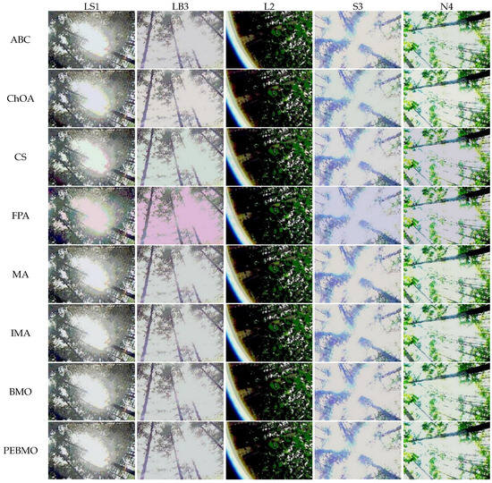
Figure 30.
Results of the segmentation of each algorithm for a threshold number of 4.
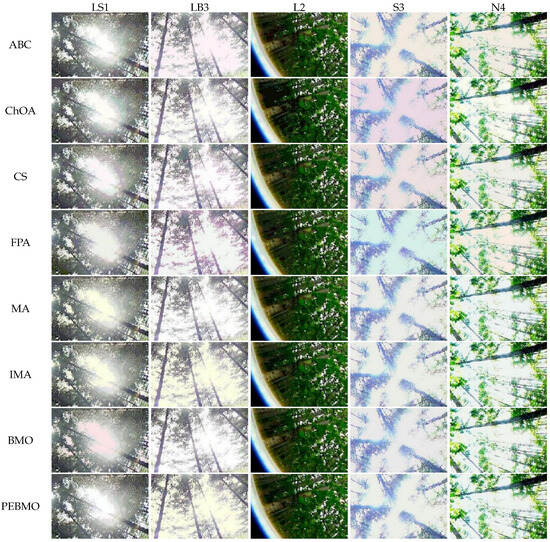
Figure 31.
Results of the segmentation of each algorithm for a threshold number of 8.

Figure 32.
Results of the segmentation of each algorithm for a threshold number of 12.
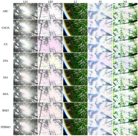
Figure 33.
Results of the segmentation of each algorithm for a threshold number of 16.
From Figure 30, it can be seen that the segmentation quality of each algorithm is poor when the number of thresholds is 4. For the non-uniform canopy images LS1 and LB3, the difficulty of segmentation is in the light and dark junction; how to make the junction area accurately segmented is an excellent test for the algorithms. All the algorithms showed mis-segmentation, and some tiny branches and leaves were wrongly divided into the sky. The same is-segmentation also occurs in the N4 image; even though N4 is a normal illumination canopy image but limited by the shooting method (elevation), there are some uneven illumination phenomena in the ideal sample with uniform illumination, to a greater or lesser extent. On the low illumination canopy image L2, the algorithms misclassify the trees and branches at low places into the background. The strong illumination image S3 has the worst segmentation quality, which appears clear and blurred with low contrast. The FPA algorithm has the worst segmentation quality and shows severe colour distortion on both LB3 and S3.
The segmentation quality in Figure 31 is visually significantly better than in Figure 30. Some minute details have not yet been successfully segmented. The FPA algorithm shows a significant improvement in segmentation quality on LB3. While colour distortion still occurs on S3. The strong light image S3 is challenging for the segmentation algorithms. The ChOA, CS and FPA algorithms show colour distortion at a threshold number of 8. The segmentation results for threshold 12 and threshold 16 have little difference in subjective visualization, and the difference is hardly noticeable, which is also consistent with the objective evaluation index. As the number of thresholds increases, the computational complexity increases exponentially. It is more challenging for intelligent algorithms. The less-performing CS and FPA algorithms still cannot segment LB3 and S3 images accurately at high thresholds. While the other algorithms improve the segmentation quality significantly, the details hidden in the glare and darkness are accurately segmented. For example, on the L2 image, the trees at the lowest brightness can be accurately segmented, and the details of tree trunks, leaves, and ground are clearly visible.
The PEMBO algorithm demonstrates better segmentation quality and stability when segmenting different types of canopy images. Especially at low thresholds, better segmentation results can be obtained even when the comparison algorithms all show more serious segmentation errors. The PEBMO algorithm shows good stability and no colour distortion at any threshold.
4. Discussion
The results of the subjective and objective evaluations of each algorithm on the four types of forest canopy images show that the proposed PEBMO algorithm has obvious advantages over other intelligent algorithms and improved intelligent algorithms. The effectiveness of the improved PEBMO algorithm is demonstrated. However, there is no perfect algorithm to solve these problems. A canopy image has a significant gap in the complexity of the target, light intensity, and image clarity, which is a significant challenge to the accuracy and stability of image segmentation.
Image segmentation accuracy: 17 equal sets of optimal fitness values emerged in acquiring fitness values, of which 94.12% were distributed when the number of thresholds was 4. This stems from the fact that none of the algorithms can accurately segment the canopy image when the number of thresholds is not big enough, and the difference between the adaptative values obtained is insignificant. As the number of thresholds increases, the differences between the algorithms are gradually noticeable. The PEBMO and IMA algorithms have apparent advantages, 40.28% and 30.56% better than the other algorithms, respectively; 90.9% and 81.36% better than BMO and MA algorithms. It shows that it is necessary to improve the intelligent algorithms to improve the segmentation accuracy of canopy images. Although the PEBMO algorithm 56.36% outperforms IMA. However, the IMA algorithm outperforms PEBMO by 69.23% and 66.67% in segmenting strong and normal light canopy images. This indicates that the PEBMO algorithm has higher segmentation accuracy in segmenting non-uniform and low-illuminated canopy images. At the same time, IMA excels in the segmentation of strong and normal light canopy images. The other algorithms perform poorly in segmentation accuracy, and only MA obtains two optimal adaptation values.
Image segmentation stability: the PEBMO algorithm has better stability in segmenting the forest canopy image, obtaining 55.56% of the optimal standard deviation value. The IMA algorithm is 79.17% better than the MA algorithm, although it only obtains 23.61% of the optimal standard deviation value. It shows that the IMA algorithm’s improvement strategy effectively improves the MA algorithm’s segmentation stability algorithm. ABC, ChOA, CS, FPA, MA, and BMO algorithms perform in general and fluctuate more in segmenting non-uniform and strongly illuminated canopy images. This is due to the difficulty of segmenting non-uniform and strongly illuminated canopy images. Uneven illumination and details hidden under strong light can easily cause poorly performing algorithms to fall into local optima and fail in segmenting such images. Hence, there is less stability in segmenting such images.
Feature similarity analysis: The optimal SSIM values obtained by ABC, ChOA, CS, FPA, MA, IMA, BMO, and PEBMO are 5, 3, 4, 3, 4, 19, 7, and 27, respectively. Of which are 1, 1, 2, 2, 1, 1, 1, 3, and 13 on the non-uniform canopy images; on low-illumination canopy images are 1, 0, 1, 1, 1, 1, 3, 1, 8; on strong light canopy images are 2, 0, 1, 0, 1, 6, 2, 4; and on normal illumination canopy images are 1, 2, 0, 0, 1, 1, 9, 1, 2. Regarding the optimal SSIM values distribution, the overall IMA and PEBMO algorithms have a clear advantage, obtaining 63.89% of the optimal SSIM values. IMA’s strengths are centered on strong and normally illuminated canopy images, while the PEBMO algorithm outperforms the comparison algorithm on non-uniform and low-illumination canopy images. The performance of the other algorithms is rather mediocre.
Degree of image distortion: the ABC, ChOA, CS, PFA, MA, IMA, BMO, and PEBMO algorithms obtained 4, 2, 4, 3, 5, 19, 6, and 29 optimal PSNR values, respectively. The IMA and PEBMO algorithms outperformed the others, indicating that their segmented canopy images were less distorted and of better quality. The performance of the algorithms on non-uniform canopy images is more balanced. The PEBMO algorithm obtains 10 out of 24 optimal values on non-uniform canopy images, which is slightly better than the comparison algorithms. The PEBMO algorithm has a clear advantage in low-illumination canopy images, obtaining 62.5% of the optimal PSNR values. In contrast, the MA and CS algorithms are slightly inferior, obtaining two optimal values, respectively. In the strong and normal illumination images, the IMA algorithm obtained 14 optimal values, while the PEBMO algorithm obtained 8, indicating that the IMA algorithm segmented images with better quality.
Feature similarity analysis: 6.94%, 2.78%, 2.78%, 5.56%, 9.72%, 15.28%, 30.56%, and 33.33% of the optimal FSIM values were obtained for ABC, ChOA, CS, FPA, MA, BMO, IMA and PEBMO, respectively. MA and BMO algorithms outperform ABC, ChOA, CS, and FPA, which indicates that they also have good optimization-seeking performance. IMA and PEBMO improve the FSIM values of both MA and BMO by 73.61%. Therefore, it is essential to increase the feature similarity between the segmentated canopy image and the original one by improving the performance of the intelligent algorithms.
Image segmentation efficiency: by analyzing the computation time data of each algorithm, it can be concluded that all algorithms take no more than 5s when the number of thresholds increases from 4 to 16. The limitation that the computational complexity increases exponentially with increasing the number of thresholds in multi-threshold segmentation is overcome. The FPA, CS, and ChOA algorithms have apparent advantages. The MA and IMA algorithms have the lowest segmentation efficiency, which is inferior to the others. The gap between the BMO and PEBMO algorithms is not large, which suggests that improving the PEBMO algorithm does not increase the segmentation efficiency of the BMO algorithm. The segmentation efficiency of ABC is between that of PEBMO and MA.
Comparison with deep learning segmentation methods: in comparison with deep learning methods, the PEBMO algorithm outperforms deep learning methods in terms of fitness value, standard deviation value, FSIM, and computation time, while deep learning outperforms the PEBMO algorithm in terms of SSIM and PSNR. Both algorithms have advantages and disadvantages. Deep learning has a clear advantage in segmentation quality. However, it also has the limitations of poor stability and high data dependency. The PEBMO algorithm, on the contrary, is stable, computationally efficient, and easy to implement. Still, it also suffers from significant performance degradation in low-dimensional or complex cases and high distortion.
In further research, overall, the PBEMO algorithm is better than the IMA algorithm, but its advantage is mainly concentrated in non-uniform and low-illumination canopy images. The IMA algorithm is 53.126% better than the PEBMO algorithm in segmenting normal illumination and strong illumination images. Therefore, further improvement of the BMO algorithm is necessary to improve its segmentation accuracy on high-brightness canopy images. In addition, this study provides a comprehensive comparison with the deep learning segmentation method, in which both algorithms have strengths and weaknesses. Deep learning has apparent advantages in segmentation quality. However, it also has the limitations of poor stability and excessive dependence on data, while the PEBMO algorithm is the opposite, with good stability, high computational efficiency, and ease of implementation. Therefore, different segmentation methods can be used based on these requirements.
5. Conclusions
This paper proposes a method to segment forest canopy images using Kapur entropy combined with the PEBMO algorithm. Compared with the segmentation results of ABC, ChOA, CS, FPA, MA, IMA, and BMO, the segmentation efficiency of the PEBMO algorithm is not as good as that of ChOA, CS, and FPA. Still, it has apparent advantages in segmentation accuracy and stability. The PEBOM and BMO algorithms are not significantly different in segmentation efficiency, which indicates that the improvement of the PEBMO algorithm does not increase the complexity of the BMO algorithm. In addition, the PEBMO algorithm was comprehensively compared with the deep learning segmentation method. The PEBMO algorithm is superior to the deep learning method in terms of the segmentation accuracy, stability, feature similarity, and efficiency. In contrast, the deep learning method was superior to the PEBMO algorithm in terms of structural similarity and image distortion. The two segmentation methods are short. Because this study only focused on small samples of canopy images, it lacked practical validation using large-scale datasets. In contrast, deep learning-based segmentation methods have the advantage of handling large-scale datasets.
Author Contributions
X.Z. and L.Z. contributed to the idea of this paper; X.Z. performed the experiments; W.X. and A.M.E.M. analyzed data; X.Z. wrote the manuscript; X.Z. and L.Z. contributed to the revision of this study. All authors have read and agreed to the published version of the manuscript.
Funding
This research was funded by Basic Research Expenses of Heilongjiang Provincial Universities (Grant No. YWF10236240135) and the Fundamental National Key R&D Program of China under Grant 2021YFC2202502.
Informed Consent Statement
This article does not contain studies with human participants or animals. Statement of informed consent is not applicable since the manuscript does not contain any patient data.
Data Availability Statement
The data used to support the findings of this study are available from https://pan.baidu.com/s/1pxT8oE5Rb5m3inopu0O7Gw?pwd=pn9b (accessed on 23 January 2025), password: c395.
Acknowledgments
The authors thank the anonymous reviewers for their useful comments that improved the quality of the paper.
Conflicts of Interest
The authors declare no conflicts of interest.
Appendix A
Table A1.
Mean fitness values for different N values.
Table A1.
Mean fitness values for different N values.
| Function | PEBMO | PEBMO | PEBMO | PEBMO | PEBMO | PEBMO | PEBMO |
|---|---|---|---|---|---|---|---|
| 8.54E + 02 | |||||||
| 3.02E + 03 | |||||||
Table A2.
Standard deviation values for different N values.
Table A2.
Standard deviation values for different N values.
| Function | PEBMO | PEBMO | PEBMO | PEBMO | PEBMO | PEBMO | PEBMO |
|---|---|---|---|---|---|---|---|
Table A3.
Mean fitness values for different T-values.
Table A3.
Mean fitness values for different T-values.
| Function | PEBMO | PEBMO | PEBMO | PEBMO | PEBMO | PEBMO | PEBMO |
|---|---|---|---|---|---|---|---|
| (T = 1000) | |||||||
Table A4.
Standard deviation values for different T-values.
Table A4.
Standard deviation values for different T-values.
| Function | PEBMO | PEBMO | PEBMO | PEBMO | PEBMO | PEBMO | PEBMO |
|---|---|---|---|---|---|---|---|
| (T = 1000) | |||||||
Table A5.
Mean fitness value of each algorithm.
Table A5.
Mean fitness value of each algorithm.
| Function | IBMO [32] | IBMO [33] | IBMO [34] | IBMO [35] | IBMO [36] | BMO | PEBMO |
|---|---|---|---|---|---|---|---|
Table A6.
Standard deviation values of each algorithm.
Table A6.
Standard deviation values of each algorithm.
| Function | IBMO [32] | IBMO [33] | IBMO [34] | IBMO [35] | IBMO [36] | BMO | PEBMO |
|---|---|---|---|---|---|---|---|
Table A7.
p-values of the Wilcoxon rank-sum test over 30 runs.
Table A7.
p-values of the Wilcoxon rank-sum test over 30 runs.
| Function | [32] | [33] | [34] | [35] | [36] | |
|---|---|---|---|---|---|---|
| 0.010763 | ||||||
| 0.025101 | ||||||
| 0.037782 | ||||||
| 4.7445E-06 | ||||||
| 0.039167 | ||||||
| 0.027086 | 0.040595 | |||||
| 0.043584 | 0.032651 | |||||
| 0.043584 | 0.046756 | |||||
| 0.045146 | ||||||
| 0.048413 | 0.023243 | |||||
| 0.040595 | 0.029205 | 0.039167 | 0.030317 | |||
| 0.026077 | 0.032651 | 0.021506 | 0.040595 | |||
| 0.042067 | ||||||
| 8.4848E-09 | ||||||
| 0.013272 | ||||||
| 0.013832 | ||||||
Table A8.
Optimal fitness values obtained by each algorithm.
Table A8.
Optimal fitness values obtained by each algorithm.
| Image | Dim | ABC | ChOA | CS | FPA | MA | IMA | BMO | PEBMO |
|---|---|---|---|---|---|---|---|---|---|
| LS1 | 4 | 48.0086 | 47.9661 | 47.7049 | 47.5568 | 48.0145 | 48.0159 | 48.0159 | 48.0159 |
| 8 | 79.2815 | 78.4253 | 77.2884 | 77.1758 | 79.8274 | 79.82757 | 79.8011 | 79.8336 | |
| 12 | 104.7496 | 102.9617 | 101.5882 | 102.2865 | 106.2248 | 106.2445 | 105.2567 | 106.2499 | |
| 16 | 126.2755 | 123.3417 | 120.5088 | 121.867 | 129.0688 | 129.1405 | 129.0721 | 129.3424 | |
| LS2 | 4 | 48.318 | 48.264 | 48.1137 | 47.7903 | 48.3211 | 48.3252 | 48.3204 | 48.3238 |
| 8 | 79.8587 | 79.299 | 77.8174 | 76.8721 | 80.4522 | 80.4494 | 80.4415 | 80.4532 | |
| 12 | 104.5855 | 102.9147 | 100.4812 | 100.7449 | 106.867 | 107.0246 | 105.1117 | 107.0272 | |
| 16 | 125.9141 | 124.7758 | 121.9272 | 120.6541 | 129.3555 | 129.8391 | 129.5242 | 129.9012 | |
| LS3 | 4 | 47.089 | 47.0635 | 46.8658 | 46.7165 | 47.0974 | 47.0974 | 47.0143 | 47.0974 |
| 8 | 77.7139 | 77.3476 | 75.947 | 74.7763 | 78.3275 | 78.2703 | 78.3124 | 78.339 | |
| 12 | 102.1062 | 100.8328 | 97.3349 | 98.2392 | 103.7293 | 103.72 | 103.4798 | 103.6359 | |
| 16 | 123.2746 | 122.903 | 120.0128 | 120.8741 | 128.0451 | 127.6188 | 125.9931 | 127.9746 | |
| LB1 | 4 | 46.2099 | 46.1422 | 45.9228 | 45.7896 | 46.2168 | 46.2172 | 46.2168 | 46.2172 |
| 8 | 76.2824 | 75.6662 | 73.7629 | 74.2691 | 76.9955 | 77.0169 | 76.13 | 77.0028 | |
| 12 | 101.1045 | 99.5656 | 97.6718 | 98.2685 | 102.7173 | 102.9983 | 102.8093 | 103.0667 | |
| 16 | 122.0963 | 121.4659 | 120.6648 | 117.8679 | 127.4983 | 128.2044 | 126.5449 | 127.6949 | |
| LB2 | 4 | 46.0391 | 45.9648 | 45.6301 | 45.5101 | 46.0496 | 46.0496 | 46.0483 | 46.0496 |
| 8 | 76.9162 | 76.2294 | 75.0841 | 74.6257 | 77.5274 | 77.5943 | 77.491 | 77.596 | |
| 12 | 101.6975 | 101.3461 | 97.4157 | 98.2788 | 103.5888 | 103.7153 | 103.006 | 103.9161 | |
| 16 | 123.1056 | 121.6342 | 119.1038 | 120.5048 | 127.4749 | 127.1375 | 127.182 | 127.2849 | |
| LB3 | 4 | 49.081 | 49.0397 | 48.9094 | 48.631 | 49.0918 | 49.0918 | 49.0915 | 49.0918 |
| 8 | 80.4904 | 79.8217 | 79.0943 | 77.1859 | 81.0314 | 81.0337 | 81.016 | 81.047 | |
| 12 | 105.2572 | 104.1442 | 101.7131 | 100.3685 | 107.6818 | 107.5712 | 107.3766 | 107.7648 | |
| 16 | 125.4144 | 125.4449 | 121.534 | 122.3018 | 130.4694 | 130.7899 | 129.6344 | 130.7112 | |
| L1 | 4 | 48.5012 | 48.4373 | 48.3292 | 47.9622 | 48.51 | 48.51 | 48.51 | 48.51 |
| 8 | 80.0675 | 79.7374 | 78.6066 | 77.4614 | 80.6704 | 80.6945 | 80.6597 | 80.6946 | |
| 12 | 105.7694 | 105.1358 | 102.1743 | 102.7151 | 108.0408 | 107.7356 | 107.7697 | 108.0403 | |
| 16 | 127.7735 | 125.6091 | 125.4105 | 126.1313 | 131.6222 | 131.5283 | 131.8409 | 132.1093 | |
| L2 | 4 | 48.4221 | 48.3408 | 47.9585 | 48.1355 | 48.4322 | 48.4322 | 48.4322 | 48.4322 |
| 8 | 80.4402 | 79.6785 | 78.0003 | 78.6101 | 80.9598 | 80.9672 | 80.9255 | 80.9789 | |
| 12 | 105.8806 | 105.632 | 103.7626 | 103.8049 | 108.3114 | 108.3499 | 108.3412 | 108.5285 | |
| 16 | 127.7982 | 126.5144 | 124.2342 | 125.7799 | 132.4709 | 132.5962 | 131.1821 | 132.6609 | |
| L3 | 4 | 47.7785 | 47.7218 | 47.531 | 47.2409 | 47.7874 | 47.7874 | 47.7874 | 47.7874 |
| 8 | 79.5244 | 79.1182 | 77.575 | 77.0088 | 79.9421 | 79.9612 | 79.9567 | 79.9768 | |
| 12 | 105.1771 | 103.9931 | 103.0118 | 103.7187 | 107.4628 | 107.4741 | 107.2843 | 107.4685 | |
| 16 | 126.706 | 126.0217 | 126.1506 | 124.2492 | 131.3893 | 131.5671 | 130.75 | 131.5785 | |
| L4 | 4 | 49.1875 | 49.1585 | 49.0315 | 48.6721 | 49.1927 | 49.1927 | 49.1927 | 49.1927 |
| 8 | 81.4676 | 81.2848 | 79.8282 | 79.317 | 81.9774 | 81.979 | 81.9695 | 81.9818 | |
| 12 | 107.5178 | 107.0374 | 105.0405 | 105.057 | 109.6753 | 109.6923 | 109.3656 | 109.7259 | |
| 16 | 129.5379 | 127.1497 | 124.2868 | 123.9073 | 133.6504 | 133.6855 | 133.2264 | 133.6386 | |
| S1 | 4 | 49.338 | 49.3001 | 48.9188 | 49.0775 | 49.3421 | 49.3421 | 49.3421 | 49.3421 |
| 8 | 81.4013 | 80.9903 | 79.8724 | 79.9943 | 81.8839 | 81.8842 | 81.8731 | 81.8842 | |
| 12 | 107.2292 | 105.4543 | 104.5251 | 102.8939 | 108.842 | 109.1382 | 108.8739 | 109.1467 | |
| 16 | 128.408 | 127.7292 | 125.9984 | 123.7531 | 132.8784 | 133 | 132.465 | 132.8416 | |
| S2 | 4 | 39.1209 | 38.9972 | 38.5964 | 38.3374 | 39.1818 | 39.1782 | 39.1488 | 38.9676 |
| 8 | 62.0115 | 61.3552 | 59.5001 | 59.9369 | 62.9102 | 63.0693 | 62.5815 | 62.3881 | |
| 12 | 78.7681 | 76.7631 | 73.3395 | 73.244 | 81.3689 | 81.5577 | 80.2543 | 78.3173 | |
| 16 | 89.8799 | 86.9816 | 84.7803 | 82.0442 | 96.2297 | 96.2723 | 91.8726 | 91.7885 | |
| S3 | 4 | 49.468 | 49.4192 | 49.1355 | 49.2403 | 49.4779 | 49.4779 | 49.4763 | 49.4779 |
| 8 | 81.5856 | 81.4717 | 80.2728 | 79.1026 | 82.3089 | 82.3113 | 82.2931 | 82.3125 | |
| 12 | 107.6504 | 106.7669 | 105.3293 | 103.3981 | 109.5594 | 109.8243 | 109.6236 | 109.7859 | |
| 16 | 129.7214 | 126.7394 | 127.524 | 125.7382 | 133.478 | 133.679 | 132.2654 | 133.3721 | |
| S4 | 4 | 47.7766 | 47.7406 | 47.5347 | 47.3725 | 47.7835 | 47.7836 | 47.7835 | 47.7836 |
| 8 | 79.5835 | 79.4014 | 77.3646 | 78.057 | 80.0262 | 80.0219 | 80.0264 | 80.0651 | |
| 12 | 106.0834 | 105.1352 | 103.3057 | 103.4634 | 107.7611 | 107.8908 | 107.7554 | 107.8515 | |
| 16 | 127.2673 | 126.7021 | 124.6762 | 125.0253 | 131.3905 | 132.014 | 130.9904 | 132.0132 | |
| N1 | 4 | 47.8655 | 47.8356 | 47.6618 | 47.5819 | 47.8747 | 47.8747 | 47.8743 | 47.8747 |
| 8 | 79.799 | 79.4778 | 77.5963 | 78.3729 | 80.2989 | 80.3078 | 80.287 | 80.2688 | |
| 12 | 105.7812 | 104.1394 | 101.5682 | 104.6089 | 107.8763 | 107.8225 | 107.8454 | 107.9298 | |
| 16 | 127.3402 | 126.3404 | 124.1978 | 124.4306 | 131.7924 | 132.0332 | 131.1746 | 131.8597 | |
| N2 | 4 | 47.8495 | 47.8201 | 47.526 | 47.4187 | 47.856 | 47.856 | 47.8529 | 47.856 |
| 8 | 105.8145 | 104.6116 | 103.3116 | 102.5263 | 107.5417 | 107.5732 | 107.5117 | 107.5868 | |
| 12 | 104.872 | 105.0269 | 101.9968 | 103.167 | 106.9648 | 107.307 | 106.6086 | 107.301 | |
| 16 | 127.37 | 126.7299 | 123.601 | 124.8646 | 131.0551 | 131.3882 | 129.7893 | 131.2023 | |
| N3 | 4 | 47.8233 | 47.7513 | 47.5664 | 47.5903 | 47.8288 | 47.8288 | 47.8286 | 47.8288 |
| 8 | 79.817 | 79.4437 | 78.367 | 78.437 | 80.2674 | 80.2788 | 80.2493 | 80.276 | |
| 12 | 105.8145 | 104.6116 | 103.3116 | 102.5263 | 107.5417 | 107.5732 | 107.5117 | 107.5868 | |
| 16 | 127.2122 | 125.8929 | 125.1016 | 123.9052 | 131.2522 | 131.4418 | 130.6177 | 131.3901 | |
| N4 | 4 | 47.7639 | 47.7441 | 47.6013 | 47.4509 | 47.7752 | 47.7752 | 47.775 | 47.774 |
| 8 | 79.8112 | 79.2091 | 78.241 | 77.9421 | 80.2766 | 80.2818 | 80.2677 | 80.2831 | |
| 12 | 105.4597 | 104.7805 | 102.5258 | 103.3431 | 107.6039 | 107.622 | 107.2717 | 107.6099 | |
| 16 | 127.0776 | 125.3874 | 122.243 | 123.5945 | 131.158 | 131.3819 | 130.6546 | 131.1936 |
Table A9.
Standard deviation values obtained by each algorithm.
Table A9.
Standard deviation values obtained by each algorithm.
| Image | Dim | ABC | ChOA | CS | FPA | MA | IMA | BMO | PEBMO |
|---|---|---|---|---|---|---|---|---|---|
| LS1 | 4 | 9.5913E-04 | 8.1216E-02 | 6.6639E-02 | 4.3741E-02 | 3.3326E-02 | 2.2291E-02 | 1.2497E-03 | 1.0414E-02 |
| 8 | 6.0017E-02 | 2.0291E-02 | 6.2622E-02 | 3.6112E-02 | 5.8858E-02 | 4.3839E-02 | 3.1330E-02 | 2.5475E-02 | |
| 12 | 3.1345E-02 | 6.7002E-02 | 8.1548E-02 | 4.3356E-02 | 9.4256E-02 | 5.3314E-02 | 3.5781E-02 | 3.4839E-03 | |
| 16 | 2.1172E-01 | 4.3651E-02 | 7.8594E-02 | 8.5891E-02 | 6.5116E-02 | 6.0465E-02 | 5.5038E-02 | 4.6511E-03 | |
| LS2 | 4 | 9.9558E-02 | 4.1407E-03 | 4.0976E-02 | 5.6743E-03 | 6.6753E-03 | 2.0703E-03 | 2.9489E-03 | 1.0351E-03 |
| 8 | 4.7812E-02 | 5.6159E-02 | 5.7359E-02 | 7.7959E-02 | 3.9974E-02 | 1.0355E-02 | 3.0926E-02 | 1.7269E-02 | |
| 12 | 4.0536E-02 | 5.7343E-02 | 5.6543E-02 | 7.7624E-02 | 8.8753E-02 | 5.5329E-02 | 5.0172E-02 | 2.7418E-02 | |
| 16 | 4.5392E-02 | 5.6343E-02 | 5.8725E-02 | 673624E-02 | 8.3723E-02 | 8.0915E-02 | 7.5231E-02 | 2.6332E-02 | |
| LS3 | 4 | 7.5542E-03 | 6.7764E-03 | 6.7653E-02 | 6.5531E-02 | 5.6642E-01 | 3.8864E-02 | 2.7784E-02 | 2.3354E-03 |
| 8 | 4.7753E-02 | 7.6534E-02 | 8.8253E-02 | 6.8843E-02 | 6.8263E-02 | 3.8862E-04 | 2.0032E-02 | 1.6603E-02 | |
| 12 | 3.7735E-02 | 5.7363E-02 | 6.8826E-02 | 7.9272E-02 | 6.6253E-02 | 6.8262E-02 | 3.7724E-02 | 2.8028E-02 | |
| 16 | 4.7363E-01 | 6.9273E-02 | 6.5615E-02 | 7.8223E-02 | 8.6635E-02 | 4.7363E-02 | 5.3836E-02 | 3.9038E-02 | |
| LB1 | 4 | 1.2346E-02 | 6.0606E-02 | 5.8373E-01 | 4.7364E-03 | 4.8834E-03 | 6.7736E-04 | 6.6363E-03 | 6.4921E-03 |
| 8 | 5.7754E-02 | 6.7734E-02 | 73635E-02 | 8.6637E-02 | 5.7733E-02 | 4.8836E-02 | 3.6625E-02 | 1.8181E-02 | |
| 12 | 2.9734E-02 | 4.8836E-02 | 1.0050E-02 | 5.8836E-02 | 7.8853E-02 | 5.7733E-02 | 4.9835E-02 | 1.7339E-02 | |
| 16 | 2.8875E-01 | 4.9986E-02 | 6.9958E-02 | 6.8874E-02 | 5.7765E-02 | 5.9987E-02 | 4.9973E-02 | 4.4096E-02 | |
| LB2 | 4 | 1.7464E-02 | 8.7464E-01 | 8.7363E-03 | 1.3032E-03 | 2.8836E-02 | 2.9983E-02 | 1.9383E-01 | 1.8336E-03 |
| 8 | 5.7736E-02 | 4.7764E-02 | 5.9974E-02 | 7.9986E-02 | 5.9982E-02 | 3.6684E-02 | 3.8862E-02 | 1.6774E-02 | |
| 12 | 7.6648E-02 | 5.7753E-02 | 4.9972E-02 | 6.8874E-02 | 5.8845E-02 | 4.9935E-02 | 3.0093E-02 | 2.5025E-02 | |
| 16 | 1.9927E-01 | 5.9942E-02 | 6.8845E-02 | 7.9974E-02 | 4.0083E-02 | 5.9973E-02 | 4.9984E-02 | 3.9933E-02 | |
| LB3 | 4 | 1.1266E-02 | 5.0096E-01 | 4.8971E-03 | 3.8875E-02 | 3.9985E-02 | 4.0097E-02 | 5.8876E-02 | 1.2222E-02 |
| 8 | 7.8874E-02 | 7.9945E-02 | 9.8875E-02 | 5.9984E-02 | 6.7789E-02 | 8.9975E-02 | 3.9984E-02 | 1.7262E-02 | |
| 12 | 6.9986E-02 | 6.9975E-02 | 9.9983E-02 | 5.9985E-02 | 6.0096E-02 | 2.8865E-02 | 4.0086E-02 | 3.3675E-02 | |
| 16 | 5.8875E-02 | 7.8874E-02 | 8.0096E-02 | 7.0065E-02 | 5.9985E-02 | 4.9975E-02 | 3.7008E-02 | 2.5764E-02 | |
| L1 | 4 | 1.0515E-02 | 8.6635E-02 | 7.8836E-03 | 5.8863E-03 | 4.8836E-03 | 3.8836E-02 | 2.0036E-01 | 1.0309E-03 |
| 8 | 7.8837E-02 | 6.9973E-02 | 6.0083E-02 | 1.2394E-02 | 5.7639E-02 | 4.0082E-02 | 3.9927E-02 | 1.7553E-02 | |
| 12 | 4.8837E-02 | 5.8837E-02 | 8.0083E-02 | 4.9937E-02 | 5.9937E-02 | 1.9973E-02 | 3.6645E-02 | 2.3773E-02 | |
| 16 | 4.9947E-01 | 6.0937E-02 | 5.0093E-02 | 6.8836E-02 | 9.8736E-02 | 7.9937E-02 | 4.9937E-02 | 2.1343E-02 | |
| L2 | 4 | 1.2636E-02 | 1.0526E-02 | 8.8837E-01 | 6.8837E-01 | 5.9937E-01 | 6.0038E-01 | 8.9936E-01 | 2.8888E-03 |
| 8 | 5.9954E-02 | 7.7732E-02 | 4.9974E-02 | 5.0085E-02 | 6.0085E-02 | 4.0999E-05 | 2.9776E-02 | 1.4833E-02 | |
| 12 | 4.0096E-02 | 6.9985E-02 | 6.9999E-02 | 5.7732E-02 | 2.5806E-02 | 3.9975E-02 | 3.1432E-02 | 2.9094E-02 | |
| 16 | 2.0997E-01 | 4.8875E-02 | 4.9874E-02 | 6.9958E-02 | 6.8864E-02 | 3.8874E-02 | 5.8874E-02 | 3.1204E-02 | |
| L3 | 4 | 1.5297E-02 | 8.9951E-02 | 7.8875E-02 | 4.9986E-01 | 4.8753E-01 | 2.2986E-01 | 2.0097E-01 | 1.8831E-03 |
| 8 | 4.7764E-02 | 9.9975E-02 | 7.0085E-02 | 8.0084E-02 | 5.7753E-02 | 4.8853E-02 | 1.3764E-02 | 9.8874E-02 | |
| 12 | 3.8846E-02 | 5.8474E-02 | 6.8846E-02 | 5.8456E-02 | 8.0048E-02 | 6.0048E-02 | 4.0484E-02 | 2.3032E-02 | |
| 16 | 3.9634E-02 | 5.8846E-02 | 6.9937E-02 | 6.8836E-02 | 8.9937E-02 | 4.0938E-02 | 3.3037E-02 | 2.9874E-02 | |
| L4 | 4 | 9.5567E-03 | 6.8474E-02 | 7.9938E-02 | 5.0847E-02 | 4.9937E-01 | 3.9374E-01 | 2.4746E-01 | 1.0162E-03 |
| 8 | 4.9975E-02 | 5.9974E-02 | 8.8874E-02 | 7.8863E-02 | 6.9975E-02 | 7.2312E-03 | 8.9984E-03 | 7.7937E-03 | |
| 12 | 4.9977E-02 | 6.9937E-02 | 8.9937E-02 | 6.0083E-02 | 4.0037E-02 | 8.0037E-02 | 4.9373E-02 | 2.2557E-02 | |
| 16 | 4.0085E-02 | 8.8852E-02 | 4.0964E-02 | 7.8853E-02 | 6.9964E-02 | 4.8863E-02 | 3.0874E-02 | 2.4199E-02 | |
| S1 | 4 | 9.3306E-03 | 8.8751E-03 | 6.0085E-02 | 5.9974E-01 | 4.9986E-02 | 2.9987E-01 | 3.0096E-02 | 1.0131E-03 |
| 8 | 6.0096E-03 | 5.0086E-03 | 8.9985E-03 | 7.0096E-03 | 4.0096E-03 | 3.7799E-03 | 4.0986E-03 | 3.9973E-03 | |
| 12 | 5.8863E-02 | 9.8866E-02 | 7.8864E-02 | 4.9974E-02 | 6.9984E-02 | 7.0085E-02 | 3.0654E-02 | 2.4505E-02 | |
| 16 | 4.9975E-02 | 5.0974E-02 | 7.9974E-02 | 9.8864E-02 | 5.8874E-02 | 6.9985E-03 | 5.0094E-02 | 3.3372E-02 | |
| S2 | 4 | 6.9986E-02 | 7.9974E-02 | 5.8864E-02 | 6.9962E-02 | 1.2251E-02 | 8.9984E-02 | 7.6543E-02 | 5.3598E-02 |
| 8 | 4.6547E-02 | 7.9734E-02 | 5.0936E-02 | 4.9464E-02 | 8.8464E-02 | 5.0494E-02 | 4.0383E-02 | 2.0789E-02 | |
| 12 | 4.0986E-02 | 5.0986E-02 | 6.8754E-02 | 5.3096E-02 | 6.0974E-02 | 5.0964E-03 | 4.2132E-02 | 3.0986E-02 | |
| 16 | 5.0843E-02 | 7.0886E-02 | 7.3124E-02 | 6.0864E-02 | 5.9753E-02 | 4.0986E-02 | 3.2643E-02 | 2.7643E-02 | |
| S3 | 4 | 8.6991E-03 | 7.7647E-03 | 7.0837E-03 | 4.7474E-03 | 2.9384E-01 | 2.9336E-02 | 2.2393E-02 | 1.6162E-03 |
| 8 | 5.8764E-02 | 7.9642E-02 | 6.2345E-02 | 5.2364E-02 | 4.3425E-02 | 3.6742E-02 | 1.0974E-01 | 1.0935E-02 | |
| 12 | 4.0875E-02 | 5.9865E-02 | 4.8657E-02 | 6.8464E-02 | 6.0383E-02 | 4.0293E-02 | 2.7397E-02 | 3.0854E-02 | |
| 16 | 3.0384E-01 | 5.0484E-02 | 6.0383E-02 | 4.9373E-02 | 7.4041E-02 | 6.0827E-02 | 3.0283E-02 | 2.4372E-02 | |
| S4 | 4 | 9.2204E-03 | 8.3636E-03 | 6.2467E-03 | 6.3029E-02 | 3.2038E-01 | 2.4038E-01 | 1.4735E-01 | 1.4647E-03 |
| 8 | 4.8753E-02 | 7.9764E-02 | 7.8975E-02 | 5.0975E-02 | 4.9543E-02 | 1.7478E-02 | 9.0985E-02 | 2.4906E-01 | |
| 12 | 7.6753E-02 | 6.9854E-02 | 8.5753E-02 | 9.6425E-02 | 6.9876E-02 | 5.0861E-03 | 4.6874E-02 | 2.8757E-02 | |
| 16 | 3.9865E-02 | 5.1352E-02 | 6.3548E-02 | 6.1253E-02 | 8.0913E-02 | 7.2414E-02 | 6.0164E-02 | 2.7668E-02 | |
| N1 | 4 | 8.1573E-03 | 7.2837E-03 | 7.3928E-03 | 3.2283E-01 | 3.0393E-02 | 2.9303E-02 | 2.5039E-02 | 1.6701E-03 |
| 8 | 4.8765E-02 | 8.9753E-02 | 6.8754E-02 | 6.7542E-02 | 5.8654E-02 | 1.6864E-02 | 1.8444E-01 | 1.8973E-02 | |
| 12 | 5.0764E-02 | 7.8753E-02 | 8.9753E-02 | 7.0864E-02 | 5.1531E-02 | 5.3642E-02 | 4.2742E-02 | 2.9642E-02 | |
| 16 | 2.7839E-01 | 5.2093E-02 | 5.5837E-02 | 7.3836E-02 | 7.1037E-02 | 1.8363E-02 | 4.3974E-02 | 3.3247E-02 | |
| N2 | 4 | 1.3807E-02 | 1.0438E-02 | 7.8364E-03 | 5.2028E-02 | 4.9374E-02 | 2.0383E-01 | 2.5052E-03 | 2.4937E-02 |
| 8 | 4.0384E-02 | 5.0384E-02 | 6.4863E-02 | 4.8645E-02 | 4.2018E-02 | 4.3927E-02 | 4.5937E-02 | 1.3767E-02 | |
| 12 | 4.2028E-02 | 7.0283E-02 | 7.3746E-02 | 8.8363E-02 | 7.5927E-02 | 5.8374E-02 | 3.2027E-02 | 1.9626E-02 | |
| 16 | 5.0373E-02 | 6.4303E-02 | 6.5927E-02 | 8.0274E-02 | 8.3484E-02 | 6.9273E-03 | 5.0273E-02 | 3.4351-02 | |
| N3 | 4 | 1.0879E-02 | 7.7373E-03 | 6.4746E-02 | 3.3648E-02 | 3.0393E-01 | 2.7393E-02 | 2.4938E-02 | 1.0453E-03 |
| 8 | 5.3038E-02 | 7.3746E-02 | 8.2937E-02 | 6.0375E-02 | 4.6937E-02 | 5.9474E-02 | 3.8354E-02 | 1.2453E-02 | |
| 12 | 4.8645E-02 | 5.2937E-02 | 6.4373E-02 | 7.4528E-02 | 4.0384E-02 | 1.9745E-02 | 3.3046E-02 | 2.6977E-02 | |
| 16 | 4.0384E-02 | 5.8464E-02 | 5.2947E-02 | 6.0484E-02 | 8.3746E-02 | 4.0173E-02 | 3.6037E-02 | 2.6190E-02 | |
| N4 | 4 | 1.2159E-02 | 6.0682E-02 | 5.8262E-03 | 4.8373E-02 | 1.8832E-03 | 3.5838E-02 | 3.9453E-02 | 2.3846E-02 |
| 8 | 6.9374E-02 | 7.1835E-02 | 7.7253E-02 | 6.9363E-02 | 5.6383E-02 | 4.9337E-02 | 3.6937E-02 | 1.2635E-02 | |
| 12 | 3.8363E-02 | 5.6383E-02 | 7.3725E-02 | 8.0373E-02 | 7.9373E-02 | 6.8332E-03 | 3.2984E-02 | 2.8832E-02 | |
| 16 | 4.7545E-02 | 5.9334E-02 | 6.3835E-02 | 7.3854E-02 | 4.7663E-02 | 4.0936E-02 | 3.6303E-02 | 2.3904E-02 |
Table A10.
SSIM values obtained by each algorithm.
Table A10.
SSIM values obtained by each algorithm.
| LS1 | 4 | 0.7209 | 0.72041 | 0.70679 | 0.71316 | 0.7192 | 0.72365 | 0.72451 | 0.72366 |
| 8 | 0.81394 | 0.81254 | 0.8159 | 0.8032 | 0.82009 | 0.82608 | 0.81812 | 0.82698 | |
| 12 | 0.86021 | 0.87064 | 0.89263 | 0.91309 | 0.89585 | 0.88353 | 0.90316 | 0.89082 | |
| 16 | 0.92534 | 0.93719 | 0.9052 | 0.94332 | 0.90512 | 0.92546 | 0.91668 | 0.95507 | |
| LS2 | 4 | 0.77999 | 0.77693 | 0.75927 | 0.78285 | 0.77617 | 0.77833 | 0.78099 | 0.7759 |
| 8 | 0.85729 | 0.86113 | 0.86577 | 0.8381 | 0.85615 | 0.85905 | 0.85471 | 0.85818 | |
| 12 | 0.90617 | 0.87217 | 0.90774 | 0.91228 | 0.90354 | 0.89829 | 0.90026 | 0.93189 | |
| 16 | 0.92607 | 0.90026 | 0.92724 | 0.95448 | 0.93401 | 0.94814 | 0.94043 | 0.95487 | |
| LS3 | 4 | 0.70844 | 0.70338 | 0.68467 | 0.7068 | 0.70876 | 0.70875 | 0.70096 | 0.71061 |
| 8 | 0.81385 | 0.81051 | 0.80819 | 0.80746 | 0.81686 | 0.8272 | 0.81795 | 0.84149 | |
| 12 | 0.90099 | 0.9152 | 0.91567 | 0.90829 | 0.91489 | 0.92039 | 0.92065 | 0.93225 | |
| 16 | 0.90983 | 0.89826 | 0.92373 | 0.9445 | 0.92906 | 0.94626 | 0.94148 | 0.94616 | |
| LB1 | 4 | 0.67413 | 0.67647 | 0.63471 | 0.66604 | 0.6755 | 0.67636 | 0.67655 | 0.67646 |
| 8 | 0.80718 | 0.78172 | 0.81787 | 0.78877 | 0.80161 | 0.80412 | 0.82123 | 0.81574 | |
| 12 | 0.90259 | 0.89423 | 0.87223 | 0.91554 | 0.92326 | 0.91254 | 0.90375 | 0.92138 | |
| 16 | 0.93583 | 0.91194 | 0.92891 | 0.93286 | 0.94553 | 0.94941 | 0.94295 | 0.9513 | |
| LB2 | 4 | 0.71374 | 0.72897 | 0.68797 | 0.69843 | 0.71162 | 0.71147 | 0.7125 | 0.71154 |
| 8 | 0.86059 | 0.82713 | 0.85647 | 0.83107 | 0.84257 | 0.84424 | 0.84883 | 0.84406 | |
| 12 | 0.92004 | 0.9099 | 0.89476 | 0.89494 | 0.91749 | 0.92029 | 0.91291 | 0.92354 | |
| 16 | 0.94308 | 0.9498 | 0.9415 | 0.93511 | 0.95108 | 0.95476 | 0.94685 | 0.961 | |
| LB3 | 4 | 0.7237 | 0.71715 | 0.73343 | 0.72454 | 0.72074 | 0.72069 | 0.72131 | 0.72078 |
| 8 | 0.81763 | 0.80184 | 0.81218 | 0.82187 | 0.82209 | 0.82212 | 0.82128 | 0.82868 | |
| 12 | 0.87506 | 0.816 | 0.86323 | 0.87579 | 0.86494 | 0.88007 | 0.88103 | 0.89334 | |
| 16 | 0.91178 | 0.90782 | 0.91396 | 0.90424 | 0.90056 | 0.90849 | 0.91602 | 0.92955 | |
| L1 | 4 | 0.79944 | 0.78747 | 0.79309 | 0.80102 | 0.79911 | 0.79916 | 0.79915 | 0.7993 |
| 8 | 0.88484 | 0.87513 | 0.88975 | 0.8719 | 0.88712 | 0.89344 | 0.89539 | 0.88715 | |
| 12 | 0.93672 | 0.91776 | 0.91026 | 0.92789 | 0.94223 | 0.93488 | 0.94229 | 0.94893 | |
| 16 | 0.92965 | 0.93076 | 0.93272 | 0.94774 | 0.95019 | 0.96024 | 0.95576 | 0.96085 | |
| L2 | 4 | 0.78368 | 0.78069 | 0.76358 | 0.76148 | 0.78193 | 0.78171 | 0.78171 | 0.78185 |
| 8 | 0.89037 | 0.87212 | 0.87899 | 0.87134 | 0.88128 | 0.883 | 0.88387 | 0.89283 | |
| 12 | 0.89247 | 0.90719 | 0.91242 | 0.91067 | 0.92242 | 0.9302 | 0.92607 | 0.93647 | |
| 16 | 0.94157 | 0.92202 | 0.92002 | 0.93117 | 0.94762 | 0.95013 | 0.941 79 | 0.94609 | |
| L3 | 4 | 0.77518 | 0.76438 | 0.78455 | 0.77297 | 0.77418 | 0.77412 | 0.7742 | 0.77438 |
| 8 | 0.85874 | 0.84941 | 0.85805 | 0.86547 | 0.86907 | 0.87367 | 0.86328 | 0.89335 | |
| 12 | 0.91441 | 0.92022 | 0.92322 | 0.91332 | 0.91776 | 0.93102 | 0.91909 | 0.93653 | |
| 16 | 0.93372 | 0.91368 | 0.92028 | 0.94585 | 0.9562 | 0.9555 | 0.93065 | 0.95704 | |
| L4 | 4 | 0.82196 | 0.81989 | 0.80929 | 0.82211 | 0.82327 | 0.82307 | 0.82312 | 0.8233 |
| 8 | 0.89617 | 0.8993 | 0.88036 | 0.88761 | 0.90449 | 0.9038 | 0.90383 | 0.90422 | |
| 12 | 0.92658 | 0.92037 | 0.91277 | 0.90874 | 0.92958 | 0.93158 | 0.92902 | 0.93037 | |
| 16 | 0.92118 | 0.92259 | 0.92976 | 0.93377 | 0.94642 | 0.94943 | 0.94629 | 0.94519 | |
| S1 | 4 | 0.79044 | 0.78916 | 0.78278 | 0.77501 | 0.79026 | 0.79007 | 0.79019 | 0.7902 |
| 8 | 0.86464 | 0.86199 | 0.84322 | 0.86664 | 0.87537 | 0.87562 | 0.87544 | 0.87566 | |
| 12 | 0.90922 | 0.8849 | 0.91588 | 0.92138 | 0.92267 | 0.92023 | 0.92559 | 0.91965 | |
| 16 | 0.93986 | 0.94155 | 0.9165 | 0.94261 | 0.93625 | 0.94349 | 0.94236 | 0.94215 | |
| S2 | 4 | 0.74587 | 0.74563 | 0.76359 | 0.73645 | 0.7555 | 0.75683 | 0.75723 | 0.75167 |
| 8 | 0.85443 | 0.82264 | 0.80746 | 0.84623 | 0.84835 | 0.86039 | 0.85681 | 0.85417 | |
| 12 | 0.9096 | 0.87075 | 0.88171 | 0.8445 | 0.91162 | 0.89509 | 0.9075 | 0.91285 | |
| 16 | 0.90528 | 0.88803 | 0.92328 | 0.91175 | 0.9302 | 0.93878 | 0.93332 | 0.93576 | |
| S3 | 4 | 0.83177 | 0.82701 | 0.81709 | 0.83111 | 0.83133 | 0.83119 | 0.83129 | 0.83128 |
| 8 | 0.89552 | 0.89054 | 0.87439 | 0.90022 | 0.90632 | 0.90661 | 0.90491 | 0.90588 | |
| 12 | 0.91878 | 0.91021 | 0.90511 | 0.91017 | 0.93189 | 0.93398 | 0.93484 | 0.93149 | |
| 16 | 0.93203 | 0.92656 | 0.92255 | 0.93413 | 0.9432 | 0.94329 | 0.94434 | 0.94727 | |
| S4 | 4 | 0.8326 | 0.83271 | 0.81437 | 0.82581 | 0.83299 | 0.83305 | 0.83293 | 0.83328 |
| 8 | 0.91445 | 0.91145 | 0.87831 | 0.90492 | 0.91652 | 0.91658 | 0.91428 | 0.91647 | |
| 12 | 0.93988 | 0.93424 | 0.92756 | 0.92549 | 0.94712 | 0.94898 | 0.94369 | 0.94795 | |
| 16 | 0.95606 | 0.94156 | 0.94257 | 0.94812 | 0.96009 | 0.95985 | 0.94511 | 0.94685 | |
| N1 | 4 | 0.82476 | 0.82638 | 0.82013 | 0.81048 | 0.82404 | 0.82372 | 0.82368 | 0.82384 |
| 8 | 0.90785 | 0.90836 | 0.90864 | 0.90145 | 0.90909 | 0.90966 | 0.90221 | 0.90609 | |
| 12 | 0.93165 | 0.93162 | 0.94224 | 0.92944 | 0.94764 | 0.94846 | 0.94766 | 0.94679 | |
| 16 | 0.94201 | 0.9468 | 0.9411 | 0.93828 | 0.96164 | 0.96478 | 0.95875 | 0.96024 | |
| N2 | 4 | 0.84303 | 0.8388 | 0.84121 | 0.83065 | 0.84145 | 0.84262 | 0.84196 | 0.84162 |
| 8 | 0.95053 | 0.93447 | 0.93441 | 0.95303 | 0.95881 | 0.95519 | 0.9574 | 0.95759 | |
| 12 | 0.93823 | 0.9443 | 0.93118 | 0.9382 | 0.95049 | 0.95317 | 0.95881 | 0.9509 | |
| 16 | 0.95628 | 0.94914 | 0.94013 | 0.9595 | 0.96596 | 0.97214 | 0.9584 | 0.96962 | |
| N3 | 4 | 0.85748 | 0.84639 | 0.8571 | 0.8506 | 0.8572 | 0.85702 | 0.85691 | 0.8598 |
| 8 | 0.92271 | 0.91404 | 0.90503 | 0.92103 | 0.92691 | 0.92832 | 0.92819 | 0.92725 | |
| 12 | 0.95053 | 0.93447 | 0.93441 | 0.95303 | 0.95519 | 0.95881 | 0.9574 | 0.95759 | |
| 16 | 0.95666 | 0.94329 | 0.94722 | 0.96194 | 0.96935 | 0.96942 | 0.96693 | 0.96697 | |
| N4 | 4 | 0.84067 | 0.84131 | 0.82968 | 0.82762 | 0.8367 | 0.83668 | 0.83753 | 0.83606 |
| 8 | 0.91293 | 0.90312 | 0.90426 | 0.91402 | 0.91399 | 0.91516 | 0.91106 | 0.9127 | |
| 12 | 0.93876 | 0.93478 | 0.93471 | 0.94267 | 0.94439 | 0.94629 | 0.94618 | 0.95286 | |
| 16 | 0.94471 | 0.93488 | 0.95145 | 0.95583 | 0.96163 | 0.97338 | 0.9565 | 0.96398 |
Table A11.
PSNR values obtained by each algorithm.
Table A11.
PSNR values obtained by each algorithm.
| Image | Dim | ABC | ChOA | CS | FPA | MA | IMA | BMO | PEBMO |
|---|---|---|---|---|---|---|---|---|---|
| LS 1 | 4 | 17.6233 | 17.5314 | 16.7462 | 17.6533 | 17.6233 | 17.6546 | 17.6227 | 17.6314 |
| 8 | 22.6606 | 22.2666 | 21.3939 | 20.7137 | 22.1226 | 22.3241 | 23.275 | 21.2806 | |
| 12 | 24.7934 | 25.3982 | 25.1572 | 24.721 | 24.8754 | 24.3582 | 25.4977 | 25.5312 | |
| 16 | 28.4347 | 27.2658 | 26.3327 | 28.0931 | 26.5375 | 27.1182 | 26.5893 | 28.9935 | |
| LS2 | 4 | 17.3107 | 17.5656 | 15.5857 | 17.6138 | 17.4985 | 17.1321 | 16.7503 | 17.138 |
| 8 | 23.5077 | 23.4514 | 20.7865 | 21.328 | 21.5137 | 21.5287 | 21.5068 | 21.5758 | |
| 12 | 26.3244 | 23.2305 | 25.5912 | 24.9803 | 24.544 | 24.5541 | 26.4788 | 24.7528 | |
| 16 | 27.0119 | 26.2853 | 25.867 | 26.5227 | 26.0105 | 26.7947 | 26.3838 | 28.2071 | |
| LS3 | 4 | 16.899 | 16.5886 | 16.8356 | 16.9682 | 16.9008 | 16.9066 | 16.4037 | 16.936 |
| 8 | 22.638 | 22.7319 | 21.7719 | 21.7665 | 23.1613 | 22.7127 | 23.2133 | 23.6906 | |
| 12 | 23.9628 | 26.7086 | 25.8549 | 24.0146 | 26.9739 | 25.3499 | 27.5647 | 27.1342 | |
| 16 | 27.8686 | 27.6627 | 27.0907 | 27.975 | 28.6953 | 30.9185 | 30.0886 | 28.9575 | |
| LB1 | 4 | 16.347 | 16.3106 | 14.5494 | 15.8343 | 16.338 | 16.3679 | 16.3628 | 16.3735 |
| 8 | 22.3389 | 20.7777 | 23.0246 | 20.396 | 22.0868 | 22.2374 | 22.9416 | 22.8365 | |
| 12 | 27.0492 | 25.7607 | 24.4119 | 25.4867 | 28.7167 | 27.8912 | 28.058 | 27.5096 | |
| 16 | 27.961 | 27.6693 | 27.2149 | 28.3347 | 30.3771 | 30.7835 | 30.373 | 30.7994 | |
| LB2 | 4 | 17.0365 | 17.646 | 16.0829 | 16.3367 | 17.0308 | 17.0229 | 17.0404 | 17.0288 |
| 8 | 24.3443 | 22.2848 | 23.4562 | 21.9288 | 22.8195 | 22.8411 | 22.9015 | 22.8438 | |
| 12 | 27.1613 | 26.1043 | 24.029 | 25.6698 | 26.2325 | 26.2385 | 26.7604 | 27.1785 | |
| 16 | 27.8746 | 28.593 | 27.2179 | 26.7854 | 28.1259 | 28.3738 | 29.3956 | 29.9283 | |
| LB3 | 4 | 16.521 | 17.0229 | 16.3612 | 16.5709 | 16.5641 | 17.1904 | 16.5184 | 16.5772 |
| 8 | 22.7803 | 22.5045 | 21.5908 | 21.4871 | 23.5517 | 22.5135 | 23.53 | 22.5442 | |
| 12 | 24.3849 | 23.2298 | 22.2403 | 22.7708 | 24.0018 | 24.2922 | 25.9828 | 26.7508 | |
| 16 | 26.97 | 27.5437 | 26.7835 | 26.2494 | 26.5026 | 26.6673 | 25.9095 | 27.9759 | |
| L1 | 4 | 19.0818 | 18.8724 | 16.6503 | 19.2056 | 19.0971 | 19.1177 | 19.1174 | 19.1248 |
| 8 | 23.9845 | 23.7547 | 20.7953 | 22.7214 | 25.1535 | 24.9971 | 25.1872 | 24.934 | |
| 12 | 26.7557 | 26.8244 | 24.0943 | 26.3993 | 28.474 | 28.7492 | 27.897 | 28.4827 | |
| 16 | 29.344 | 27.8012 | 26.5161 | 29.6275 | 30.2466 | 30.6045 | 30.2709 | 30.9262 | |
| L2 | 4 | 19.214 | 18.934 | 18.4822 | 18.2934 | 19.28 | 19.2661 | 19.2314 | 19.2611 |
| 8 | 24.6821 | 23.9745 | 24.3752 | 23.2947 | 25.1417 | 25.1001 | 25.1898 | 25.2418 | |
| 12 | 26.9997 | 26.8935 | 25.6933 | 26.6686 | 28.648 | 28.6753 | 28.3863 | 28.7201 | |
| 16 | 28.4252 | 29.0059 | 26.8518 | 28.3103 | 30.9197 | 31.2622 | 29.8385 | 31.3071 | |
| L3 | 4 | 19.0855 | 18.6216 | 19.863 | 18.5664 | 19.1691 | 19.1448 | 19.1571 | 19.1681 |
| 8 | 24.4603 | 24.3383 | 22.1891 | 22.079 | 24.6038 | 24.894 | 24.7713 | 24.9318 | |
| 12 | 27.6851 | 25.8301 | 26.9509 | 27.8983 | 28.4691 | 28.6442 | 28.4195 | 28.4659 | |
| 16 | 29.1044 | 28.6716 | 26.3205 | 28.7242 | 30.5994 | 30.9194 | 30.052 | 31.1223 | |
| L4 | 4 | 18.8011 | 18.8275 | 19.1015 | 18.4389 | 18.8672 | 18.84 | 18.8983 | 18.8256 |
| 8 | 24.4402 | 24.5406 | 21.7447 | 23.6505 | 25.047 | 25.0946 | 24.9973 | 25.1384 | |
| 12 | 24.8287 | 26.9375 | 25.683 | 27.1285 | 28.5027 | 28.5998 | 27.7892 | 28.6067 | |
| 16 | 27.3812 | 28.5217 | 25.7337 | 26.4747 | 30.7057 | 30.8145 | 29.6389 | 30.9529 | |
| S1 | 4 | 18.8215 | 18.8977 | 18.7729 | 18.7698 | 18.9078 | 18.8915 | 18.8955 | 18.9285 |
| 8 | 24.9591 | 24.6393 | 23.2686 | 23.8365 | 25.1517 | 25.1536 | 25.1225 | 25.0951 | |
| 12 | 27.0805 | 26.9384 | 23.8944 | 26.6772 | 28.2633 | 28.5538 | 28.2944 | 28.7182 | |
| 16 | 28.2425 | 28.255 | 28.0888 | 29.7205 | 30.9566 | 31.1797 | 30.5167 | 31.1172 | |
| S2 | 4 | 20.5159 | 20.2824 | 20.4582 | 20.2603 | 20.7525 | 20.8226 | 20.6059 | 20.5969 |
| 8 | 24.9453 | 24.3096 | 23.6766 | 25.3071 | 25.4971 | 25.9313 | 26.019 | 26.2151 | |
| 12 | 28.0797 | 26.4541 | 26.1149 | 25.1395 | 29.0762 | 28.6297 | 29.1504 | 28.7945 | |
| 16 | 29.1548 | 28.1465 | 28.3377 | 29.8636 | 30.6961 | 31.3226 | 29.9611 | 31.1449 | |
| S3 | 4 | 18.5082 | 17.8457 | 17.403 | 18.3808 | 18.2577 | 18.1328 | 18.1228 | 18.241 |
| 8 | 23.0315 | 21.7351 | 21.3589 | 23.4432 | 23.2565 | 23.5103 | 22.9768 | 23.7055 | |
| 12 | 24.8746 | 27.2904 | 23.8472 | 24.57 | 27.146 | 28.2448 | 27.3182 | 27.9499 | |
| 16 | 26.7708 | 28.3615 | 27.2307 | 29.5579 | 29.7832 | 30.4554 | 27.6182 | 29.7469 | |
| S4 | 4 | 18.2151 | 19.0337 | 17.7096 | 18.0413 | 18.3834 | 18.4671 | 18.3932 | 18.4992 |
| 8 | 23.9811 | 24.4487 | 23.28 | 22.4472 | 25.036 | 25.0792 | 24.2885 | 24.8859 | |
| 12 | 27.1415 | 26.9 | 24.3046 | 27.6016 | 28.466 | 28.3352 | 28.135 | 28.5991 | |
| 16 | 28.1777 | 29.4093 | 26.5124 | 29.4189 | 31.0545 | 31.1967 | 30.5662 | 31.1365 | |
| N1 | 4 | 19.5422 | 19.2234 | 18.9259 | 18.8318 | 19.4357 | 19.3821 | 19.3507 | 19.3989 |
| 8 | 24.4604 | 23.6524 | 24.4041 | 24.8512 | 25.3394 | 25.3609 | 25.2308 | 25.5503 | |
| 12 | 26.8013 | 27.3504 | 26.4697 | 25.9722 | 28.4772 | 28.0926 | 28.3457 | 28.4018 | |
| 16 | 28.5226 | 28.4434 | 27.7891 | 28.9198 | 30.3835 | 30.6952 | 30.4121 | 30.9756 | |
| N2 | 4 | 18.6177 | 18.4094 | 18.453 | 17.8951 | 18.6733 | 18.6819 | 18.5012 | 18.7055 |
| 8 | 27.3798 | 27.0411 | 25.7212 | 26.9315 | 28.5073 | 28.6977 | 28.6039 | 28.6595 | |
| 12 | 26.5124 | 26.3507 | 24.4956 | 26.6851 | 28.6239 | 28.0661 | 27.7979 | 28.3443 | |
| 16 | 28.8253 | 27.9491 | 25.2474 | 27.5651 | 30.6305 | 30.8572 | 29.4339 | 30.6594 | |
| N3 | 4 | 19.4139 | 19.3445 | 19.6787 | 18.7282 | 19.4707 | 19.4034 | 19.4296 | 19.4436 |
| 8 | 24.7077 | 24.4412 | 24.6671 | 24.5945 | 25.1031 | 25.3984 | 25.2439 | 25.139 | |
| 12 | 27.3798 | 27.0411 | 25.7212 | 26.9315 | 28.5073 | 28.6977 | 28.6039 | 28.6595 | |
| 16 | 29.555 | 27.8668 | 26.1534 | 29.2765 | 30.6679 | 31.2805 | 29.7968 | 31.2565 | |
| N4 | 4 | 19.1838 | 19.5107 | 19.4319 | 19.2365 | 19.3237 | 19.293 | 19.3566 | 19.4714 |
| 8 | 24.197 | 24.9887 | 23.0143 | 23.1427 | 25.4654 | 25.4856 | 25.2843 | 25.503 | |
| 12 | 28.145 | 27.7777 | 27.1333 | 27.4841 | 28.7963 | 28.8931 | 28.418 | 28.7206 | |
| 16 | 27.6399 | 28.2612 | 27.0658 | 29.3758 | 30.5235 | 31.0846 | 30.5232 | 31.3229 |
Table A12.
FSIM values obtained by each algorithm.
Table A12.
FSIM values obtained by each algorithm.
| Image | Dim | ABC | ChOA | CS | FPA | MA | IMA | BMO | PEBMO |
|---|---|---|---|---|---|---|---|---|---|
| LS1 | 4 | 0.90224 | 0.90174 | 0.89546 | 0.89926 | 0.90196 | 0.90405 | 0.90409 | 0.9041 |
| 8 | 0.93672 | 0.9336 | 0.93502 | 0.93176 | 0.93954 | 0.94219 | 0.94172 | 0.93919 | |
| 12 | 0.95426 | 0.95414 | 0.96394 | 0.97328 | 0.96679 | 0.96167 | 0.96977 | 0.96414 | |
| 16 | 0.97532 | 0.9796 | 0.9674 | 0.97651 | 0.96604 | 0.96866 | 0.97276 | 0.98245 | |
| LS2 | 4 | 0.90112 | 0.8985 | 0.88896 | 0.9012 | 0.89962 | 0.90013 | 0.90121 | 0.89825 |
| 8 | 0.93886 | 0.9412 | 0.94092 | 0.92924 | 0.94088 | 0.94245 | 0.94006 | 0.94209 | |
| 12 | 0.96072 | 0.94495 | 0.95862 | 0.96385 | 0.96412 | 0.96055 | 0.96592 | 0.97683 | |
| 16 | 0.97139 | 0.95764 | 0.96885 | 0.98238 | 0.98078 | 0.98455 | 0.9844 | 0.98856 | |
| LS3 | 4 | 0.89401 | 0.88967 | 0.884 | 0.89446 | 0.89387 | 0.89408 | 0.88661 | 0.89708 |
| 8 | 0.92676 | 0.92637 | 0.91353 | 0.93126 | 0.92803 | 0.93321 | 0.92822 | 0.9248 | |
| 12 | 0.95919 | 0.96649 | 0.98563 | 0.96223 | 0.96669 | 0.96924 | 0.96665 | 0.97563 | |
| 16 | 0.96898 | 0.96459 | 0.97436 | 0.98505 | 0.9761 | 0.98591 | 0.98052 | 0.98892 | |
| LB1 | 4 | 0.86394 | 0.86353 | 0.8401 | 0.85688 | 0.8643 | 0.86482 | 0.86473 | 0.86883 |
| 8 | 0.91275 | 0.90385 | 0.92181 | 0.90043 | 0.90985 | 0.91104 | 0.92472 | 0.92137 | |
| 12 | 0.96626 | 0.96792 | 0.95296 | 0.97334 | 0.97212 | 0.97117 | 0.97108 | 0.96716 | |
| 16 | 0.98503 | 0.96931 | 0.97839 | 0.98462 | 0.98055 | 0.98858 | 0.9854 | 0.98844 | |
| LB2 | 4 | 0.8642 | 0.87295 | 0.84787 | 0.85671 | 0.8638 | 0.8638 | 0.8644 | 0.86379 |
| 8 | 0.93962 | 0.92145 | 0.9361 | 0.92563 | 0.92847 | 0.93176 | 0.93309 | 0.93379 | |
| 12 | 0.97083 | 0.96287 | 0.95803 | 0.9588 | 0.96813 | 0.9695 | 0.96312 | 0.9669 | |
| 16 | 0.97817 | 0.9854 | 0.981 | 0.975 | 0.98444 | 0.98895 | 0.96975 | 0.98943 | |
| LB3 | 4 | 0.90716 | 0.90697 | 0.90315 | 0.90858 | 0.90619 | 0.90624 | 0.90647 | 0.90634 |
| 8 | 0.94051 | 0.93447 | 0.93027 | 0.9423 | 0.94244 | 0.94231 | 0.94219 | 0.94239 | |
| 12 | 0.9583 | 0.9375 | 0.94954 | 0.95793 | 0.96112 | 0.95537 | 0.96346 | 0.96355 | |
| 16 | 0.9724 | 0.97079 | 0.97489 | 0.96988 | 0.96931 | 0.97198 | 0.97328 | 0.98367 | |
| L1 | 4 | 0.9627 | 0.95719 | 0.94878 | 0.96288 | 0.9628 | 0.96279 | 0.96282 | 0.96282 |
| 8 | 0.98594 | 0.98302 | 0.97351 | 0.97948 | 0.96836 | 0.98678 | 0.98681 | 0.98875 | |
| 12 | 0.99431 | 0.99101 | 0.98694 | 0.99151 | 0.99621 | 0.99494 | 0.99569 | 0.99622 | |
| 16 | 0.99306 | 0.99256 | 0.99076 | 0.99536 | 0.99681 | 0.99751 | 0.9972 | 0.99871 | |
| L2 | 4 | 0.95749 | 0.95596 | 0.94837 | 0.94385 | 0.95669 | 0.95659 | 0.95664 | 0.95664 |
| 8 | 0.98584 | 0.98281 | 0.98433 | 0.98187 | 0.98604 | 0.98648 | 0.98545 | 0.98578 | |
| 12 | 0.98725 | 0.98802 | 0.98849 | 0.98972 | 0.99287 | 0.99396 | 0.99472 | 0.99477 | |
| 16 | 0.99215 | 0.99198 | 0.98992 | 0.99345 | 0.99655 | 0.99667 | 0.99523 | 0.99819 | |
| L3 | 4 | 0.95823 | 0.95237 | 0.96312 | 0.95604 | 0.95826 | 0.9582 | 0.95823 | 0.95832 |
| 8 | 0.98185 | 0.98015 | 0.98377 | 0.97917 | 0.98741 | 0.98643 | 0.98329 | 0.98641 | |
| 12 | 0.99142 | 0.99283 | 0.99303 | 0.99212 | 0.99404 | 0.99599 | 0.99634 | 0.9942 | |
| 16 | 0.99484 | 0.99129 | 0.99137 | 0.99547 | 0.99776 | 0.99874 | 0.99494 | 0.99897 | |
| L4 | 4 | 0.96317 | 0.96246 | 0.95986 | 0.96272 | 0.95402 | 0.96394 | 0.96407 | 0.96389 |
| 8 | 0.98556 | 0.987 | 0.97843 | 0.98189 | 0.98929 | 0.98907 | 0.98917 | 0.98941 | |
| 12 | 0.98861 | 0.99026 | 0.98734 | 0.98688 | 0.99391 | 0.99454 | 0.99326 | 0.99366 | |
| 16 | 0.98787 | 0.99131 | 0.98513 | 0.98974 | 0.99599 | 0.99656 | 0.99554 | 0.99879 | |
| S1 | 4 | 0.95115 | 0.95088 | 0.94589 | 0.94119 | 0.95111 | 0.95212 | 0.95115 | 0.95106 |
| 8 | 0.97816 | 0.97731 | 0.96718 | 0.97904 | 0.98265 | 0.98268 | 0.98257 | 0.98274 | |
| 12 | 0.98858 | 0.98262 | 0.98526 | 0.99114 | 0.993 | 0.99472 | 0.99341 | 0.99458 | |
| 16 | 0.99409 | 0.99314 | 0.98936 | 0.99481 | 0.99494 | 0.99884 | 0.99581 | 0.9978 | |
| S2 | 4 | 0.9395 | 0.9385 | 0.94141 | 0.93436 | 0.94467 | 0.94555 | 0.94427 | 0.94312 |
| 8 | 0.98067 | 0.97174 | 0.96468 | 0.97705 | 0.97842 | 0.98027 | 0.98199 | 0.98426 | |
| 12 | 0.98958 | 0.98034 | 0.98161 | 0.96961 | 0.99083 | 0.98919 | 0.99022 | 0.9914 | |
| 16 | 0.98941 | 0.98725 | 0.98577 | 0.99098 | 0.994 | 0.9946 | 0.99215 | 0.99348 | |
| S3 | 4 | 0.94515 | 0.94072 | 0.93178 | 0.94404 | 0.94491 | 0.94493 | 0.94587 | 0.945 |
| 8 | 0.97519 | 0.96943 | 0.95708 | 0.97672 | 0.98296 | 0.98332 | 0.98193 | 0.98288 | |
| 12 | 0.98426 | 0.98324 | 0.97335 | 0.98033 | 0.99152 | 0.99032 | 0.99177 | 0.98958 | |
| 16 | 0.98759 | 0.98746 | 0.98205 | 0.98842 | 0.99229 | 0.99237 | 0.99212 | 0.99383 | |
| S4 | 4 | 0.96278 | 0.96639 | 0.94911 | 0.95928 | 0.96379 | 0.96408 | 0.96373 | 0.96412 |
| 8 | 0.98909 | 0.98857 | 0.97722 | 0.98396 | 0.99094 | 0.99596 | 0.99053 | 0.99111 | |
| 12 | 0.99429 | 0.99289 | 0.98742 | 0.98954 | 0.99549 | 0.99581 | 0.9952 | 0.99578 | |
| 16 | 0.99454 | 0.9934 | 0.99244 | 0.9944 | 0.99689 | 0.99819 | 0.99623 | 0.9974 | |
| N1 | 4 | 0.96412 | 0.9646 | 0.96037 | 0.95501 | 0.96372 | 0.96366 | 0.96345 | 0.96371 |
| 8 | 0.98929 | 0.98811 | 0.98797 | 0.98782 | 0.98994 | 0.99015 | 0.98797 | 0.98866 | |
| 12 | 0.99294 | 0.99282 | 0.99327 | 0.99005 | 0.99607 | 0.99615 | 0.99614 | 0.99579 | |
| 16 | 0.99236 | 0.99338 | 0.99436 | 0.9923 | 0.99708 | 0.99736 | 0.99658 | 0.99707 | |
| N2 | 4 | 0.96161 | 0.95999 | 0.961 | 0.95489 | 0.96125 | 0.96113 | 0.96052 | 0.96124 |
| 8 | 0.9936 | 0.9914 | 0.9897 | 0.99418 | 0.99605 | 0.99547 | 0.99584 | 0.99589 | |
| 12 | 0.99091 | 0.99216 | 0.98544 | 0.98951 | 0.99393 | 0.99488 | 0.99447 | 0.99547 | |
| 16 | 0.99468 | 0.9916 | 0.98601 | 0.99395 | 0.99647 | 0.99755 | 0.99477 | 0.99723 | |
| N3 | 4 | 0.97152 | 0.96657 | 0.97137 | 0.96818 | 0.97144 | 0.9713 | 0.97126 | 0.97139 |
| 8 | 0.98881 | 0.98612 | 0.98494 | 0.98813 | 0.9907 | 0.99122 | 0.99046 | 0.99037 | |
| 12 | 0.9936 | 0.9914 | 0.9897 | 0.99418 | 0.99605 | 0.99547 | 0.99584 | 0.99589 | |
| 16 | 0.99528 | 0.99081 | 0.99105 | 0.99501 | 0.99725 | 0.99829 | 0.99678 | 0.99691 | |
| N4 | 4 | 0.97145 | 0.97279 | 0.96758 | 0.96568 | 0.97026 | 0.97031 | 0.97068 | 0.98052 |
| 8 | 0.99051 | 0.98764 | 0.98609 | 0.9901 | 0.99042 | 0.99115 | 0.99069 | 0.99311 | |
| 12 | 0.99486 | 0.99302 | 0.99323 | 0.99418 | 0.99602 | 0.99624 | 0.98681 | 0.98617 | |
| 16 | 0.99316 | 0.99321 | 0.99496 | 0.99602 | 0.99766 | 0.998 | 0.97816 | 0.99788 |
Table A13.
Segmentation time of each algorithm.
Table A13.
Segmentation time of each algorithm.
| Image | Dim | ABC | ChOA | CS | FPA | MA | IMA | BMO | PEBMO |
|---|---|---|---|---|---|---|---|---|---|
| LS1 | 4 | 37.22928 | 17.695249 | 19.13846 | 17.740747 | 55.376535 | 37.166682 | 34.237015 | 34.936568 |
| 8 | 37.896377 | 20.091828 | 19.800877 | 18.330005 | 56.802970 | 52.277045 | 35.090928 | 35.700193 | |
| 12 | 38.771357 | 20.081655 | 19.767274 | 18.783700 | 57.793687 | 53.020603 | 36.086696 | 36.662281 | |
| 16 | 39.287938 | 21.167638 | 20.024618 | 19.365886 | 59.278632 | 53.220836 | 37.403720 | 37.588600 | |
| LS2 | 4 | 24.472916 | 11.568041 | 12.351668 | 11.664440 | 36.313718 | 33.275220 | 21.855616 | 22.503947 |
| 8 | 25.434418 | 12.831296 | 12.704705 | 12.114079 | 38.183649 | 34.817854 | 22.960178 | 23.464068 | |
| 12 | 26.215167 | 14.072158 | 12.962511 | 12.605819 | 40.183427 | 35.801986 | 23.902696 | 24.607119 | |
| 16 | 26.993187 | 15.12972 | 13.228076 | 13.169610 | 41.004110 | 37.275398 | 24.750286 | 25.635050 | |
| LS3 | 4 | 43.732545 | 20.761193 | 22.899068 | 23.091635 | 66.734566 | 68.184735 | 40.639670 | 37.083445 |
| 8 | 46.36112 | 22.782857 | 22.3491 | 23.207058 | 67.865978 | 71.922150 | 43.102734 | 37.073659 | |
| 12 | 46.34296 | 23.856602 | 23.69978 | 24.240265 | 69.502483 | 75.503281 | 44.030943 | 37.744468 | |
| 16 | 46.731358 | 25.166717 | 23.95882 | 24.376147 | 71.307433 | 87.025817 | 45.534060 | 37.811615 | |
| LB1 | 4 | 44.434293 | 21.447038 | 25.796542 | 22.616864 | 66.804753 | 60.203722 | 40.838085 | 37.412987 |
| 8 | 44.604497 | 22.566733 | 27.125672 | 23.795538 | 67.811368 | 61.627583 | 42.639474 | 38.952232 | |
| 12 | 47.062296 | 24.282379 | 26.521476 | 24.387127 | 69.780675 | 62.863945 | 43.849856 | 40.571279 | |
| 16 | 45.916378 | 25.717482 | 25.963951 | 24.924855 | 72.836444 | 64.855724 | 44.290286 | 41.891504 | |
| LB2 | 4 | 38.674422 | 18.612669 | 19.857395 | 18.615673 | 57.030461 | 52.895087 | 36.150716 | 36.255754 |
| 8 | 39.26661 | 19.720364 | 19.795959 | 19.047104 | 58.619785 | 53.409597 | 36.610783 | 37.624395 | |
| 12 | 40.002934 | 20.964177 | 20.117676 | 19.557334 | 60.179192 | 54.747048 | 37.518394 | 37.946456 | |
| 16 | 41.207668 | 21.843003 | 20.295459 | 20.086542 | 62.123606 | 57.443062 | 38.549201 | 38.342609 | |
| LB3 | 4 | 36.154416 | 17.437841 | 19.212014 | 17.377589 | 53.623489 | 49.442407 | 34.733022 | 34.122744 |
| 8 | 37.035675 | 18.787321 | 19.220966 | 19.617221 | 56.146807 | 50.991854 | 35.224510 | 37.488786 | |
| 12 | 37.55301 | 19.71797 | 19.517402 | 20.149972 | 56.629029 | 51.961767 | 36.180740 | 38.641067 | |
| 16 | 38.424474 | 20.772787 | 19.750810 | 20.794519 | 58.214680 | 53.064280 | 37.122870 | 39.799497 | |
| L1 | 4 | 41.051625 | 19.601239 | 19.887026 | 18.599911 | 56.098041 | 62.258926 | 38.973851 | 37.723193 |
| 8 | 38.860798 | 20.197736 | 21.372919 | 19.733481 | 58.145387 | 62.896369 | 40.354323 | 40.440959 | |
| 12 | 41.091415 | 22.714245 | 22.092051 | 19.949292 | 59.762912 | 63.875078 | 41.091602 | 40.153868 | |
| 16 | 42.300903 | 22.745791 | 22.799909 | 20.924924 | 63.857581 | 65.781827 | 41.163393 | 41.477621 | |
| L2 | 4 | 40.400465 | 19.267078 | 21.779027 | 20.131819 | 56.728961 | 63.029445 | 40.701435 | 39.047658 |
| 8 | 39.620052 | 20.229916 | 21.263268 | 20.387864 | 58.995829 | 64.587187 | 41.696364 | 41.619870 | |
| 12 | 42.136511 | 22.243030 | 21.039173 | 20.587864 | 62.835466 | 65.737986 | 42.376936 | 42.198586 | |
| 16 | 43.453199 | 22.712033 | 22.651821 | 21.456482 | 63.487736 | 73.036815 | 41.938681 | 42.578852 | |
| L3 | 4 | 41.651373 | 20.562473 | 20.245571 | 19.179261 | 60.488762 | 63.119181 | 38.641669 | 38.350863 |
| 8 | 41.775009 | 20.871508 | 21.185607 | 19.963350 | 60.548046 | 65.177358 | 41.196163 | 40.692544 | |
| 12 | 41.635897 | 22.493221 | 20.949466 | 20.470828 | 61.024848 | 65.465063 | 42.772323 | 41.217254 | |
| 16 | 42.891119 | 22.303059 | 21.368231 | 21.077807 | 62.604924 | 67.671144 | 42.076427 | 41.969717 | |
| L4 | 4 | 41.664035 | 17.977323 | 19.448814 | 18.689504 | 59.348059 | 60.483557 | 38.595866 | 38.164451 |
| 8 | 39.898770 | 19.251582 | 19.910049 | 19.297812 | 57.298910 | 62.569755 | 38.979198 | 40.953199 | |
| 12 | 40.411957 | 20.744578 | 20.538862 | 19.810363 | 60.965267 | 63.282028 | 39.367845 | 41.859678 | |
| 16 | 41.427593 | 21.830335 | 20.555764 | 20.290848 | 60.626087 | 64.625314 | 40.890484 | 39.671965 | |
| S1 | 4 | 41.376391 | 19.666468 | 20.820117 | 19.493075 | 55.030536 | 56.176679 | 38.254125 | 37.845036 |
| 8 | 41.776974 | 21.231476 | 21.533468 | 20.509745 | 56.221224 | 56.889929 | 38.552515 | 39.669227 | |
| 12 | 42.397796 | 22.348482 | 21.918919 | 20.869063 | 58.462701 | 60.232910 | 39.517207 | 39.984327 | |
| 16 | 44.261575 | 23.809297 | 22.061764 | 21.475511 | 58.862877 | 61.261118 | 40.841301 | 40.398811 | |
| S2 | 4 | 38.135751 | 18.188345 | 19.466423 | 18.671546 | 51.982031 | 53.564314 | 35.189187 | 35.627038 |
| 8 | 39.813595 | 19.574101 | 19.907445 | 18.927240 | 53.080718 | 55.304997 | 36.160551 | 38.292573 | |
| 12 | 40.060868 | 20.768279 | 20.047219 | 20.304747 | 54.680720 | 55.802372 | 36.845098 | 37.520523 | |
| 16 | 41.235165 | 22.526153 | 21.423369 | 19.943233 | 55.968605 | 56.724195 | 37.780194 | 38.476276 | |
| S3 | 4 | 40.569390 | 19.875454 | 20.600692 | 19.228148 | 55.622982 | 54.830691 | 36.852124 | 37.245393 |
| 8 | 41.978758 | 20.711915 | 21.572265 | 20.446739 | 56.010121 | 56.028520 | 37.983871 | 37.818678 | |
| 12 | 41.668422 | 22.042469 | 22.092151 | 20.645074 | 56.589893 | 56.678563 | 38.866153 | 38.710808 | |
| 16 | 43.176003 | 23.294215 | 22.118312 | 21.105215 | 58.334851 | 58.189914 | 39.941698 | 40.404805 | |
| S4 | 4 | 30.811501 | 14.913649 | 15.527552 | 14.510955 | 40.971292 | 49.012948 | 29.143943 | 30.413819 |
| 8 | 31.986144 | 16.060690 | 16.765421 | 15.293708 | 42.558512 | 49.985548 | 30.132220 | 30.983137 | |
| 12 | 34.073560 | 17.459489 | 16.355632 | 16.099273 | 43.987887 | 51.377949 | 29.350372 | 29.838231 | |
| 16 | 34.215684 | 18.654223 | 17.344093 | 16.620193 | 45.723299 | 53.430512 | 30.826774 | 30.601450 | |
| N1 | 4 | 48.080689 | 22.922331 | 20.640436 | 19.486808 | 60.063580 | 77.262505 | 40.261474 | 44.658027 |
| 8 | 50.057162 | 23.685717 | 20.825789 | 19.967930 | 60.138692 | 65.406769 | 41.577599 | 45.393651 | |
| 12 | 50.878197 | 25.558345 | 21.547738 | 20.513401 | 60.751766 | 65.998404 | 41.083507 | 46.317470 | |
| 16 | 52.329762 | 26.993951 | 21.767024 | 20.920336 | 57.901145 | 67.896402 | 43.236833 | 47.695611 | |
| N2 | 4 | 49.299985 | 21.336161 | 19.975253 | 18.770847 | 57.881112 | 62.017222 | 39.519407 | 42.890841 |
| 8 | 49.631489 | 24.305667 | 20.504612 | 19.314143 | 62.928686 | 63.500447 | 40.614695 | 43.604405 | |
| 12 | 49.419689 | 26.082441 | 20.609293 | 20.038289 | 62.330939 | 64.722787 | 41.166166 | 44.732965 | |
| 16 | 51.129177 | 28.068365 | 21.138693 | 20.772468 | 62.399751 | 66.099338 | 41.682694 | 46.304206 | |
| N3 | 4 | 49.159793 | 23.008118 | 20.181396 | 18.699672 | 57.426584 | 62.677785 | 37.622883 | 42.788288 |
| 8 | 48.905687 | 24.722272 | 20.614596 | 19.651256 | 58.584165 | 64.199307 | 40.480156 | 43.730899 | |
| 12 | 51.452641 | 24.925428 | 21.324635 | 19.911117 | 61.130516 | 64.897459 | 41.625435 | 44.652749 | |
| 16 | 53.609564 | 27.240178 | 21.535619 | 20.898271 | 60.452223 | 66.196937 | 41.559147 | 45.723206 | |
| N4 | 4 | 38.724639 | 18.779342 | 19.875514 | 19.188456 | 56.632000 | 62.164292 | 39.805522 | 43.034793 |
| 8 | 42.414032 | 20.078173 | 20.159491 | 19.498807 | 59.720099 | 63.055118 | 40.661501 | 43.496024 | |
| 12 | 41.785961 | 21.713797 | 20.854678 | 20.370970 | 60.218897 | 64.536068 | 41.862139 | 44.750324 | |
| 16 | 44.309302 | 22.733385 | 21.248481 | 20.533584 | 61.055662 | 65.620812 | 41.174764 | 45.087065 |
Table A14.
Comparison between PEBMO algorithm and deep learning.
Table A14.
Comparison between PEBMO algorithm and deep learning.
| Image | Dim | Fitness Value | Standard Deviation | SSIM | PSNR | FSIM | Computation Time | ||||||
|---|---|---|---|---|---|---|---|---|---|---|---|---|---|
| PEBMO | Deep | PEBMO | Deep | PEBMO | Deep | PEBMO | Deep | PEBMO | Deep | PEBMO | Deep | ||
| LS1 | 4 | 48.0159 | 0.1075 | 1.0414E-02 | 0.0325 | 0.72366 | 0.9908 | 17.6314 | 57.8183 | 0.9041 | 0.2688 | 34.936568 | 22.5598 |
| 8 | 79.8336 | 0.1204 | 2.5475E-02 | 0.0485 | 0.82698 | 0.9901 | 21.2806 | 57.3232 | 0.93919 | 0.2838 | 35.700193 | 32.9795 | |
| 12 | 106.2499 | 0.1309 | 3.4839E-03 | 0.0436 | 0.89082 | 0.9898 | 25.5312 | 56.9608 | 0.96414 | 0.2945 | 36.662281 | 57.7556 | |
| 16 | 129.3424 | 0.1319 | 4.6511E-03 | 0.0578 | 0.95507 | 0.9897 | 28.9935 | 56.9286 | 0.98245 | 0.2966 | 37.588600 | 165.7821 | |
| LS2 | 4 | 48.3238 | 0.1071 | 1.0351E-03 | 0.0185 | 0.7759 | 0.9914 | 17.138 | 57.8346 | 0.89825 | 0.2678 | 22.503947 | 22.3029 |
| 8 | 80.4532 | 0.1101 | 1.7269E-02 | 0.0654 | 0.85818 | 0.9913 | 21.5758 | 57.7131 | 0.94209 | 0.2708 | 23.464068 | 32.9847 | |
| 12 | 107.0272 | 0.1223 | 2.7418E-02 | 0.0435 | 0.93189 | 0.9908 | 24.7528 | 57.2555 | 0.97683 | 0.2845 | 24.607119 | 56.5832 | |
| 16 | 129.9012 | 0.1209 | 2.6332E-02 | 0.0356 | 0.95487 | 0.9908 | 28.2071 | 57.3072 | 0.98856 | 0.2835 | 25.635050 | 165.9812 | |
| LS3 | 4 | 47.0974 | 0.0787 | 2.3354E-03 | 0.0389 | 0.71061 | 0.9956 | 16.936 | 59.1708 | 0.89708 | 0.2218 | 37.083445 | 23.3651 |
| 8 | 78.339 | 0.1306 | 1.6603E-02 | 0.0256 | 0.84149 | 0.9879 | 23.6906 | 56.9723 | 0.9248 | 0.2969 | 37.073659 | 32.9382 | |
| 12 | 103.6359 | 0.1440 | 2.8028E-02 | 0.0364 | 0.93225 | 0.9875 | 27.1342 | 56.5467 | 0.97563 | 0.3114 | 37.744468 | 58.5183 | |
| 16 | 127.9746 | 0.1438 | 3.9038E-02 | 0.0478 | 0.94616 | 0.9875 | 28.9575 | 56.5546 | 0.98892 | 0.3106 | 37.811615 | 165.8707 | |
| LB1 | 4 | 46.2172 | 0.0765 | 6.4921E-03 | 0.0561 | 0.67646 | 0.9955 | 16.3735 | 59.2962 | 0.86883 | 0.2181 | 37.412987 | 23.2946 |
| 8 | 77.0028 | 0.1213 | 1.8181E-02 | 0.0289 | 0.81574 | 0.9891 | 22.8365 | 57.2937 | 0.92137 | 0.2842 | 38.952232 | 33.1972 | |
| 12 | 103.0667 | 0.1338 | 1.7339E-02 | 0.0328 | 0.92138 | 0.9884 | 27.5096 | 56.8673 | 0.96716 | 0.2980 | 40.571279 | 57.4462 | |
| 16 | 127.6949 | 0.1399 | 4.4096E-02 | 0.0298 | 0.9513 | 0.9883 | 30.7994 | 56.6735 | 0.98844 | 0.3047 | 41.891504 | 156.0487 | |
| LB2 | 4 | 46.0496 | 0.0630 | 1.8336E-03 | 0.0473 | 0.71154 | 0.9967 | 17.0288 | 60.1343 | 0.86379 | 0.1983 | 36.255754 | 22.2942 |
| 8 | 77.596 | 0.1182 | 1.6774E-02 | 0.0534 | 0.84406 | 0.9895 | 22.8438 | 57.4054 | 0.93379 | 0.2801 | 37.624395 | 33.1487 | |
| 12 | 103.9161 | 0.1262 | 2.5025E-02 | 0.0598 | 0.92354 | 0.9893 | 27.1785 | 57.1212 | 0.9669 | 0.2888 | 37.946456 | 56.5224 | |
| 16 | 127.2849 | 0.1297 | 3.9933E-02 | 0.0326 | 0.961 | 0.9892 | 29.9283 | 57.0029 | 0.98943 | 0.2925 | 38.342609 | 156.5286 | |
| LB3 | 4 | 49.0918 | 0.1097 | 1.2222E-02 | 0.0498 | 0.72078 | 0.9899 | 16.5772 | 57.7282 | 0.90634 | 0.2731 | 34.122744 | 23.3701 |
| 8 | 81.047 | 0.1199 | 1.7262E-02 | 0.0564 | 0.82868 | 0.9896 | 22.5442 | 57.3440 | 0.94239 | 0.2843 | 37.488786 | 33.067 | |
| 12 | 107.7648 | 0.1305 | 3.3675E-02 | 0.0425 | 0.89334 | 0.9892 | 26.7508 | 56.9757 | 0.96355 | 0.2956 | 38.641067 | 55.7509 | |
| 16 | 130.7112 | 0.1314 | 2.5764E-02 | 0.0365 | 0.92955 | 0.9892 | 27.9759 | 56.9455 | 0.98367 | 0.2970 | 39.799497 | 166.0908 | |
| L1 | 4 | 48.51 | 0.1004 | 1.0309E-03 | 0.0417 | 0.7993 | 0.9943 | 19.1248 | 58.1148 | 0.96282 | 0.2571 | 37.723193 | 22.3921 |
| 8 | 80.6946 | 0.1452 | 1.7553E-02 | 0.0513 | 0.88715 | 0.9869 | 24.934 | 56.5110 | 0.98875 | 0.3172 | 40.440959 | 33.1111 | |
| 12 | 108.0403 | 0.1675 | 2.3773E-02 | 0.056 | 0.94893 | 0.9848 | 28.4827 | 55.8894 | 0.99622 | 0.3426 | 40.153868 | 57.3989 | |
| 16 | 132.1093 | 0.1642 | 2.1343E-02 | 0.0435 | 0.96085 | 0.9861 | 30.9262 | 55.9773 | 0.99871 | 0.3359 | 41.477621 | 15.2046 | |
| L2 | 4 | 48.4322 | 0.0943 | 2.8888E-03 | 0.0429 | 0.78185 | 0.9944 | 19.2611 | 58.3835 | 0.95664 | 0.2461 | 39.047658 | 23.3232 |
| 8 | 80.9789 | 0.1362 | 1.4833E-02 | 0.0476 | 0.89283 | 0.9896 | 25.2418 | 56.7900 | 0.98578 | 0.3030 | 41.619870 | 33.2126 | |
| 12 | 108.5285 | 0.1322 | 2.9094E-02 | 0.0436 | 0.93647 | 0.9914 | 28.7201 | 56.9186 | 0.99477 | 0.2913 | 42.198586 | 58.4160 | |
| 16 | 132.6609 | 0.1835 | 3.1204E-02 | 0.0452 | 0.94609 | 0.9827 | 31.3071 | 55.4937 | 0.99819 | 0.3615 | 42.578852 | 165.8598 | |
| L3 | 4 | 47.7874 | 0.0856 | 1.8831E-03 | 0.0471 | 0.77438 | 0.9954 | 19.1681 | 58.8059 | 0.95832 | 0.2339 | 38.350863 | 23.2801 |
| 8 | 79.9768 | 0.1359 | 9.8874E-02 | 0.0386 | 0.89335 | 0.9891 | 24.9318 | 56.7980 | 0.98641 | 0.3033 | 40.692544 | 33.1594 | |
| 12 | 107.4685 | 0.1502 | 2.3032E-02 | 0.0521 | 0.93653 | 0.9870 | 28.4659 | 56.3632 | 0.9942 | 0.3204 | 41.217254 | 57.3497 | |
| 16 | 131.5785 | 0.1690 | 2.9874E-02 | 0.0298 | 0.95704 | 0.9852 | 31.1223 | 55.8527 | 0.99897 | 0.3416 | 41.969717 | 166.1911 | |
| L4 | 4 | 49.1927 | 0.0980 | 1.0162E-03 | 0.0364 | 0.8233 | 0.9940 | 18.8256 | 58.2194 | 0.96389 | 0.2547 | 38.164451 | 23.2850 |
| 8 | 81.9818 | 0.1486 | 7.7937E-03 | 0.0612 | 0.90422 | 0.9879 | 25.1384 | 56.4115 | 0.98941 | 0.3122 | 40.953199 | 33.2179 | |
| 12 | 109.7259 | 0.1758 | 2.2557E-02 | 0.0402 | 0.93037 | 0.9847 | 28.6067 | 55.6816 | 0.99366 | 0.3512 | 41.859678 | 56.3911 | |
| 16 | 133.6386 | 0.1925 | 2.4199E-02 | 0.0528 | 0.94519 | 0.9819 | 30.9529 | 55.2854 | 0.99879 | 0.3709 | 39.671965 | 159.9169 | |
| S1 | 4 | 49.3421 | 0.1416 | 1.0131E-03 | 0.0419 | 0.7902 | 0.9869 | 18.9285 | 56.6188 | 0.95106 | 0.3158 | 37.845036 | 22.2733 |
| 8 | 81.8842 | 0.1354 | 3.9973E-03 | 0.0362 | 0.87566 | 0.9892 | 25.0951 | 56.8146 | 0.98274 | 0.3022 | 39.669227 | 33.0524 | |
| 12 | 109.1467 | 0.1742 | 2.4505E-02 | 0.0408 | 0.91965 | 0.9844 | 28.7182 | 55.7213 | 0.99458 | 0.3494 | 39.984327 | 55.3965 | |
| 16 | 132.8416 | 0.1727 | 3.3372E-02 | 0.0507 | 0.94215 | 0.9845 | 31.1172 | 55.7571 | 0.9978 | 0.3486 | 40.398811 | 166.1598 | |
| S2 | 4 | 38.9676 | 0.0864 | 5.3598E-02 | 0.0317 | 0.75167 | 0.9954 | 20.5969 | 58.7680 | 0.94312 | 0.2344 | 35.627038 | 23.2570 |
| 8 | 62.3881 | 0.1655 | 2.0789E-02 | 0.0433 | 0.85417 | 0.9840 | 26.2151 | 55.9429 | 0.98426 | 0.3424 | 38.292573 | 32.9243 | |
| 12 | 78.3173 | 0.1830 | 3.0986E-02 | 0.0366 | 0.91285 | 0.9826 | 28.7945 | 55.5054 | 0.9914 | 0.3612 | 37.520523 | 58.4439 | |
| 16 | 91.7885 | 0.1876 | 2.7643E-02 | 0.0271 | 0.93576 | 0.9825 | 31.1449 | 55.3995 | 0.99348 | 0.3648 | 38.476276 | 156.9967 | |
| S3 | 4 | 49.4779 | 0.0911 | 1.6162E-03 | 0.0365 | 0.83128 | 0.9945 | 18.241 | 58.5364 | 0.945 | 0.2348 | 37.245393 | 22.2431 |
| 8 | 82.3125 | 0.2065 | 1.0935E-02 | 0.0451 | 0.90588 | 0.9793 | 23.7055 | 54.9811 | 0.98288 | 0.3579 | 37.818678 | 31.0139 | |
| 12 | 109.7859 | 0.1904 | 3.0854E-02 | 0.0432 | 0.93149 | 0.9820 | 27.9499 | 55.3351 | 0.98958 | 0.3594 | 38.710808 | 57.7750 | |
| 16 | 133.3721 | 0.1926 | 2.4372E-02 | 0.0513 | 0.94727 | 0.9816 | 29.7469 | 55.2837 | 0.99383 | 0.3581 | 40.404805 | 155.7512 | |
| S4 | 4 | 47.7836 | 0.1026 | 1.4647E-03 | 0.0614 | 0.83328 | 0.9927 | 18.4992 | 58.0212 | 0.96412 | 0.2559 | 30.413819 | 23.3486 |
| 8 | 80.0651 | 0.1047 | 1.4906E-01 | 0.0321 | 0.91647 | 0.9941 | 24.8859 | 57.9308 | 0.99111 | 0.2583 | 30.983137 | 32.983 | |
| 12 | 107.8515 | 0.1814 | 2.8757E-02 | 0.0452 | 0.94795 | 0.9832 | 28.5991 | 55.5451 | 0.99578 | 0.3598 | 29.838231 | 58.7869 | |
| 16 | 132.0132 | 0.1850 | 2.7668E-02 | 0.0355 | 0.94685 | 0.9828 | 31.1365 | 55.4587 | 0.9974 | 0.3629 | 30.601450 | 155.8123 | |
| N1 | 4 | 47.8747 | 0.0671 | 1.6701E-03 | 0.0472 | 0.82384 | 0.9973 | 19.3989 | 59.8643 | 0.96371 | 0.2043 | 44.658027 | 22.3048 |
| 8 | 80.2688 | 0.1259 | 1.8973E-02 | 0.0533 | 0.90609 | 0.9906 | 25.5503 | 57.1294 | 0.98866 | 0.2894 | 45.393651 | 32.9232 | |
| 12 | 107.9298 | 0.1567 | 2.9642E-02 | 0.0466 | 0.94679 | 0.9867 | 28.4018 | 56.1803 | 0.99579 | 0.3271 | 46.317470 | 58.4291 | |
| 16 | 131.8597 | 0.1786 | 3.3247E-02 | 0.0425 | 0.96024 | 0.9839 | 30.9756 | 55.6124 | 0.99707 | 0.3539 | 47.695611 | 16.1105 | |
| N2 | 4 | 47.856 | 0.0981 | 2.4937E-02 | 0.0512 | 0.84162 | 0.9944 | 18.7055 | 58.2133 | 0.96124 | 0.2538 | 42.890841 | 22.3614 |
| 8 | 107.5868 | 0.1200 | 1.3767E-02 | 0.0436 | 0.95759 | 0.9925 | 28.6595 | 57.3398 | 0.99589 | 0.2807 | 43.604405 | 32.9322 | |
| 12 | 107.301 | 0.1664 | 1.9626E-02 | 0.0377 | 0.9509 | 0.9862 | 28.3443 | 55.9197 | 0.99547 | 0.3369 | 44.732965 | 57.4437 | |
| 16 | 131.2023 | 0.1679 | 3.4351-02 | 0.0286 | 0.96962 | 0.9856 | 30.6594 | 55.8793 | 0.99723 | 0.3414 | 46.304206 | 155.9574 | |
| N3 | 4 | 47.8288 | 0.0702 | 1.0453E-03 | 0.0388 | 0.8598 | 0.9970 | 19.4436 | 59.6649 | 0.97139 | 0.2110 | 42.788288 | 23.3718 |
| 8 | 80.276 | 0.1129 | 1.2453E-02 | 0.0453 | 0.92725 | 0.9930 | 25.139 | 57.6030 | 0.99037 | 0.2688 | 43.730899 | 33.0735 | |
| 12 | 107.5868 | 0.1629 | 2.6977E-02 | 0.0198 | 0.95759 | 0.9858 | 28.6595 | 56.0120 | 0.99589 | 0.3366 | 44.652749 | 56.5866 | |
| 16 | 131.3901 | 0.1729 | 2.6190E-02 | 0.0421 | 0.96697 | 0.9846 | 31.2565 | 55.7538 | 0.99691 | 0.3483 | 45.723206 | 16.0879 | |
| N4 | 4 | 47.774 | 0.1158 | 2.3846E-02 | 0.0533 | 0.83606 | 0.9909 | 19.4714 | 57.4923 | 0.98052 | 0.2769 | 43.034793 | 22.3124 |
| 8 | 80.2831 | 0.1456 | 1.2635E-02 | 0.0437 | 0.9127 | 0.9870 | 25.503 | 56.4989 | 0.99311 | 0.3164 | 43.496024 | 33.0007 | |
| 12 | 107.6099 | 0.1497 | 2.8832E-02 | 0.0453 | 0.95286 | 0.9881 | 28.7206 | 56.3778 | 0.98617 | 0.3163 | 44.750324 | 57.4719 | |
| 16 | 131.1936 | 0.1618 | 2.3904E-02 | 0.0476 | 0.96398 | 0.9864 | 31.3229 | 56.0401 | 0.99788 | 0.3328 | 45.087065 | 156.0582 | |
References
- Wang, W.; Ye, C.; Pan, Z.; Tian, J. Multilevel threshold segmentation of rice plant images utilizing tuna swarm optimization algorithm incorporating quadratic interpolation and elite swarm genetic operators. Expert Syst. Appl. 2025, 263, 125673. [Google Scholar] [CrossRef]
- Abualigah, L.; Al-Okbi, N.K.; Awwad, E.M.; Sharaf, M.; Sh, M. Correction: Boosted Aquila Arithmetic Optimization Algorithm for multi-level thresholding image segmentation. Evol. Syst. 2024, 15, 1427. [Google Scholar] [CrossRef]
- Abdel-Basset, M.; Mohamed, R.; Hezam, I.M.; Sallam, K. M; Hameed, I.A. An enhanced spider wasp optimization algorithm for multilevel thresholding-based medical image segmentation. Evol. Syst. 2024, 15, 2249–2271. [Google Scholar] [CrossRef]
- Sowmiya, R.; Sathya, P.D. Hybrid leader corona virus herd optimizer with multilevel thresholding techniques for foreground and background image segmentation. Comput. Electr. Eng. 2024, 120, 109569. [Google Scholar] [CrossRef]
- Houssein, E.H.; Emam, M.M.; Singh, N.; Nagwan, M.; Samee, A.; Alabdulhafith, M.; Çelik, E. An improved honey badger algorithm for global optimization and multilevel thresholding segmentation: Real case with brain tumor images. Clust. Comput. 2024, 27, 14315–14364. [Google Scholar] [CrossRef]
- Lee, H.S.; Cho, S.I. Spatial color histogram-based image segmentation using texture-aware region merging. Multim. Tools Appl. 2022, 81, 24573–24600. [Google Scholar] [CrossRef]
- Kavitha, K.J.; Shan, P.B. Medical image watermarking based on novel encoding for EHR and fusion based morphological watershed segmentation algorithm for medical images. Multimed. Tools Appl. 2024, 83, 25163–25190. [Google Scholar] [CrossRef]
- Kwenda, C.; Gwetu, M.V.; Dombeu, J.V.F. Hybridizing Deep Neural Networks and Machine Learning Models for Aerial Satellite Forest Image Segmentation. J. Imaging 2024, 10, 132. [Google Scholar] [CrossRef]
- Capua, F.R.; Schandin, J.; Cristóforis, P.D. Training Point-Based Deep Learning Networks for Forest Segmentation with Synthetic Data. In Proceedings of the International Conference on Pattern Recognition, Kolkata, India, 1–5 December 2024; Springer Nature: Cham, Switzerland, 2024; Volume 4, pp. 64–80. [Google Scholar] [CrossRef]
- Shi, L.; Wang, G.; Mo, L.; Yi, X.; Wu, X.; Wu, P. Automatic Segmentation of Standing Trees from Forest Images Based on Deep Learning. Sensors 2022, 22, 6663. [Google Scholar] [CrossRef] [PubMed]
- Wang, M.; Wang, W.; Feng, S.; Li, L. Adaptive Multi-class Segmentation Model of Aggregate Image Based on Improved Sparrow Search Algorithm. KSII Trans. Internet Inf. Syst. 2023, 17, 391–411. [Google Scholar] [CrossRef]
- Wu, Y.; Li, Q. The Algorithm of Watershed Color Image Segmentation Based on Morphological Gradient. Sensors 2022, 22, 8202. [Google Scholar] [CrossRef] [PubMed]
- Bhandari, A.K. A novel beta differential evolution algorithm-based fast multilevel thresholding for color image segmentation. Neural Comput. Appl. 2020, 32, 4583–4613. [Google Scholar] [CrossRef]
- Jia, H.; Su, Y.; Rao, H.; Liang, M.; Abualigah, L.; Liu, C.; Chen, X. Improved artificial rabbits algorithm for global optimization and multi-level thresholding color image segmentation. Artif. Intell. Rev. 2025, 58, 55. [Google Scholar] [CrossRef]
- Olmez, Y.; Koca, G.O.; Tanyildizi, E.; Sengür, A. Multilevel image thresholding based on Renyi’s entropy and golden sinus algorithm II. Neural Comput. Appl. 2023, 35, 17837–17850. [Google Scholar] [CrossRef]
- Wu, B.; Zhu, L.; Li, X. Giza pyramids construction algorithm with gradient contour approach for multilevel thresholding color image segmentation. Appl. Intell. 2023, 53, 21248–21267. [Google Scholar] [CrossRef]
- Wu, B.; Zhu, L.; Cao, J.; Wang, J. A Hybrid Preaching Optimization Algorithm Based on Kapur Entropy for Multilevel Thresholding Color Image Segmentation. Entropy 2021, 23, 1599. [Google Scholar] [CrossRef]
- Zhao, S.; Wang, P.; Heidari, A.A.; Chen, H.; Turabieh, H.; Mafarja, M.M.; Li, C. Multilevel threshold image segmentation with diffusion association slime mould algorithm and Renyi’s entropy for chronic obstructive pulmonary disease. Comput. Biol. Med. 2021, 134, 104427. [Google Scholar] [CrossRef] [PubMed]
- Zhao, D.; Liu, L.; Yu, F.; Heidari, A.A.; Wang, M.; Oliva, D.; Muhammad, K.; Chen, H. Ant colony optimization with horizontal and vertical crossover search: Fundamental visions for multilevel thresholding image segmentation. Expert Syst. Appl. 2021, 167, 114122. [Google Scholar] [CrossRef]
- Zhang, J.; Zhang, T.; Wang, D.; Zhang, G.; Kong, M.; Li, Z.; Chen, R.; Xu, Y. A complex-valued encoding golden jackal optimization for multilevel thresholding image segmentation. Appl. Soft Comput. 2024, 165, 112108. [Google Scholar] [CrossRef]
- Chakraborty, F.; Roy, P.K. An efficient multilevel thresholding image segmentation through improved elephant herding optimization. Evol. Intell. 2025, 18, 17. [Google Scholar] [CrossRef]
- Hu, K.; Mo, Y. An efficient multi-threshold image segmentation method for COVID-19 images using reinforcement learning-based enhanced sand cat algorithm. J. Supercomput. 2025, 81, 113. [Google Scholar] [CrossRef]
- Xia, H.; Ke, Y.; Liao, R.; Sun, Y. Fractional order calculus enhanced dung beetle optimizer for function global optimization and multilevel threshold medical image segmentation. J. Supercomput. 2025, 81, 90. [Google Scholar] [CrossRef]
- Nama, S. A novel improved SMA with quasi reflection operator: Performance analysis, application to the image segmentation problem of COVID-19 chest X-ray images. Appl. Soft Comput. 2022, 118, 108483. [Google Scholar] [CrossRef]
- Wang, J.; Bei, J.; Song, H.; Zhang, H.; Zhang, P. A whale optimization algorithm with combined mutation and removing similarity for global optimization and multilevel thresholding image segmentation. Appl. Soft Comput. 2023, 137, 110130. [Google Scholar] [CrossRef]
- Houssein, E.H.; Marwa, M.; Emam, M.M.; Ali, A.A. An efficient multilevel thresholding segmentation method for thermography breast cancer imaging based on improved chimp optimization algorithm. Expert Syst. Appl. 2021, 185, 115651. [Google Scholar] [CrossRef]
- Abualigah, L.; Al-Okbi, N.K.; Elaziz, M.A.; Houssein, E.H. Boosting Marine Predators Algorithm by Salp Swarm Algorithm for Multilevel Thresholding Image Segmentation. Multim. Tools Appl. 2021, 81, 16707–16742. [Google Scholar] [CrossRef] [PubMed]
- Wu, B.; Zhu, L.; Wang, J. Forest Canopy Image Segmentation Basedon Differential Evolution Whale Optimization Algorithm. J. Northwest For. Univ. 2022, 37, 67–73. [Google Scholar] [CrossRef]
- Tong, K.; Zhu, L.; Wang, J.; Fu, X. Forest Canopy Image Segmentation Based on Improved Northern Goshawk Algorithm by Using Multi-Strategy Fusion. For. Eng. 2024, 40, 124–133. [Google Scholar] [CrossRef]
- Wang, J.; Zhu, L.; Wu, B.; Ryspayev, A. Forestry Canopy Image Segmentation Based on Improved Tuna Swarm Optimization. Forests 2022, 13, 1746. [Google Scholar] [CrossRef]
- Sulaiman, M.H.; Mustaffa, Z.; Saari, M.M.; Daniyal, H.; Daud, M.R.; Razali, S.; Mohamed, A.I. Barnacles Mating Optimizer: A Bio-Inspired Algorithm for Solving Optimization Problems. SNPD 2018, 265–270. [Google Scholar] [CrossRef]
- Mohammadnejad, Z.; Al-Khafaji, H.M.R.; Mohammed, A.S.; Alatba, S.R. Energy optimization for optimal location in 5G networks using improved Barnacles Mating Optimizer. Phys. Commun. 2023, 59, 102068. [Google Scholar] [CrossRef]
- Yang, Z.; Liu, Q.; Zhang, L.; Dai, J.; Razmjooy, N. Model parameter estimation of the PEMFCs using improved Barnacles Mating Optimization algorithm. Energy 2020, 212, 118738. [Google Scholar] [CrossRef]
- Li, H.; Zheng, G.; Sun, K.; Jiang, Z.; Li, Y.; Jia, H. A Logistic Chaotic Barnacles Mating Optimizer with Masi Entropy for Color Image Multilevel Thresholding Segmentation. IEEE Access 2020, 8, 213130–213153. [Google Scholar] [CrossRef]
- Liu, B.; Wang, H.; Tseng, M.L.; Li, Z. State of charge estimation for lithium-ion batteries based on improved barnacle mating optimizer and support vector machine. J. Energy Storage 2022, 55, 105830. [Google Scholar] [CrossRef]
- Zhao, J.; Zhang, T.; Ma, S.; Wang, M. Improved barnacles mating optimizer to solve high-dimensional continuous optimization problems. CAAI Trans. Intell. Syst. 2023, 18, 823–832. [Google Scholar] [CrossRef]
- Karaboga, D.; Basturk, B. A powerful and efficient algorithm for numerical function optimization: Artificial bee colony (ABC) algorithm. J. Glob. Optim. 2007, 39, 459–471. [Google Scholar] [CrossRef]
- Khishe, M.; Mosavi, M.R. Chimp optimization algorithm. Expert Syst. Appl. 2020, 149, 113338. [Google Scholar] [CrossRef]
- Yang, X.S.; Deb, S. Cuckoo search via levy flights. In Proceedings of the 2009 World Congress on Nature & Biologically Inspired Computing (NaBIC), Coimbatore, India, 9–11 December 2009; pp. 210–214. [Google Scholar] [CrossRef]
- Yang, X.S. Flower pollination algorithm for global optimization. In Proceedings of the International Conference on Unconventional Computing and Natural Computation (UCNC), Berlin/Heidelberg, Germany, 3–7 September 2012; Volume 7445, pp. 240–249. [Google Scholar] [CrossRef]
- Zervoudakis, K.; Tsafarakis, S. A mayfly optimization algorithm. Comput. Ind. Eng. 2020, 145, 106559. [Google Scholar] [CrossRef]
- Zhao, X.; Zhu, L.; Wu, B. An improved mayfly algorithm based on Kapur entropy for multilevel thresholding color image segmentation. J. Intell. Fuzzy Syst. 2023, 44, 365–380. [Google Scholar] [CrossRef]
- Naruei, I.; Keynia, F. A new optimization method based on COOT bird natural life model. Expert Syst. Appl. 2021, 183, 115352. [Google Scholar] [CrossRef]
- He, L.; Huang, S. An efficient krill herd algorithm for color image multilevel thresholding segmentation problem. Appl. Soft Comput. 2020, 89, 106063. [Google Scholar] [CrossRef]
- Zhao, X.; Zhu, L.; Wang, J.; Mohamed, A.M.E. Enhancement Method Based on Multi-Strategy Improved Pelican Optimization Algorithm and Application to Low-Illumination Forest Canopy Images. Forests 2024, 15, 1783. [Google Scholar] [CrossRef]
- Abualigah, L.; Almotairi, K.H.; Elaziz, M.A. Multilevel thresholding image segmentation using meta-heuristic optimization algorithms: Comparative analysis, open challenges and new trends. Appl. Intell. 2023, 53, 11654–11704. [Google Scholar] [CrossRef]
- Qiao, L.; Liu, K.; Xue, Y.; Tang, W.; Salehnia, T. A multi-level thresholding image segmentation method using hybrid Arithmetic Optimization and Harris Hawks Optimizer algorithms. Expert Syst. Appl. 2024, 241, 122316. [Google Scholar] [CrossRef]
- Yan, Z.; Zhang, J.; Yang, Z.; Tang, J. Kapur’s Entropy for Underwater Multilevel Thresholding Image Segmentation Based on Whale Optimization Algorithm. IEEE Access 2021, 9, 41294–41319. [Google Scholar] [CrossRef]
- Das, G.; Panda, R.; Samantaray, L.; Agrawal, S. A Novel Segmentation Error Minimization-Based Method for Multilevel Optimal Threshold Selection Using Opposition Equilibrium Optimizer. Int. J. Image Graph. 2023, 23, 2350021:1–2350021:22. [Google Scholar] [CrossRef]
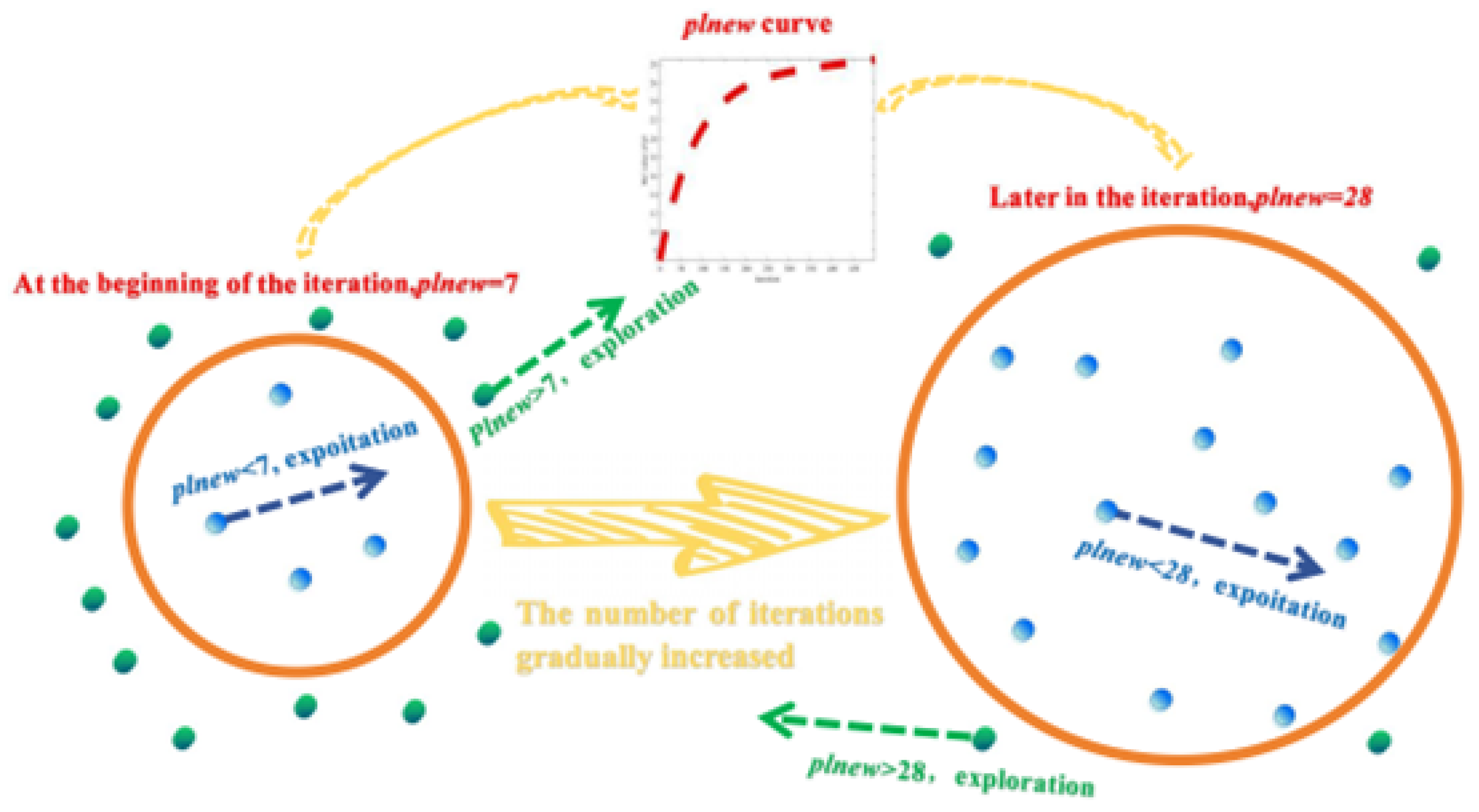
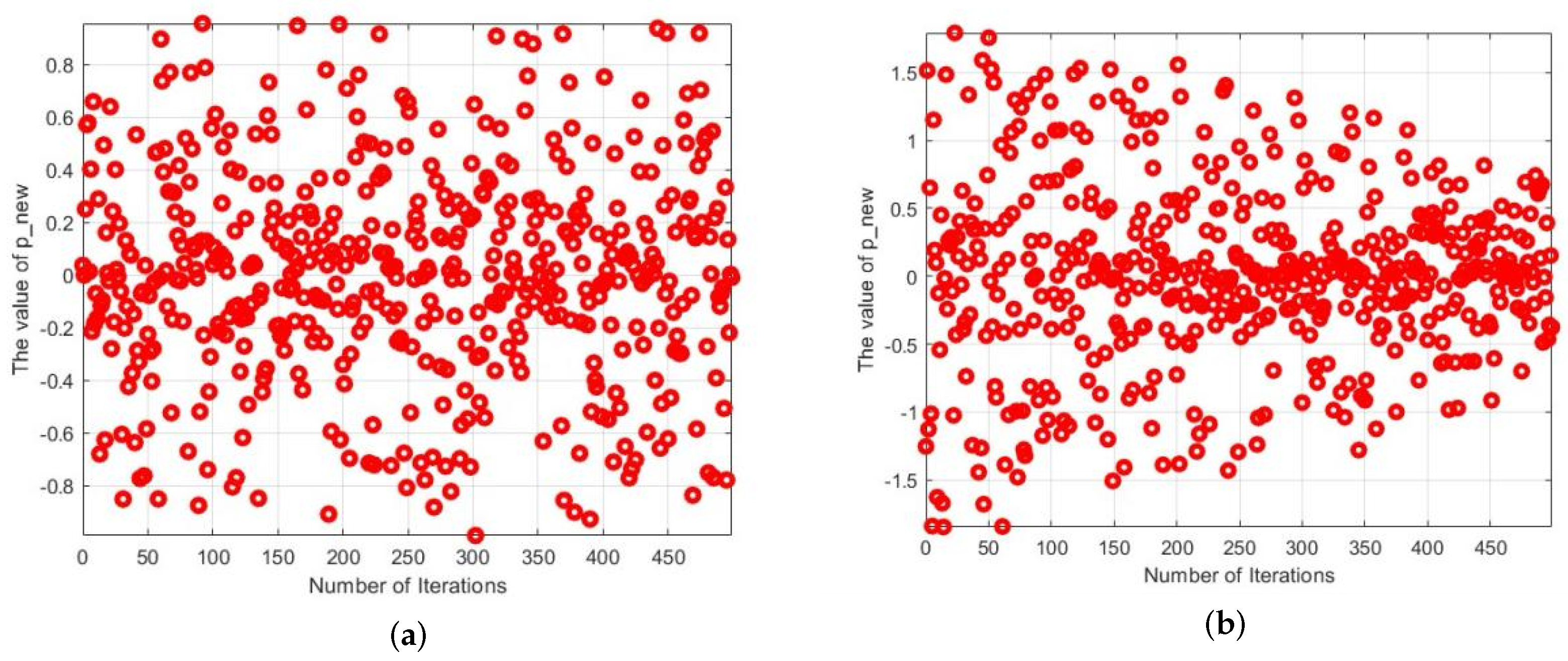

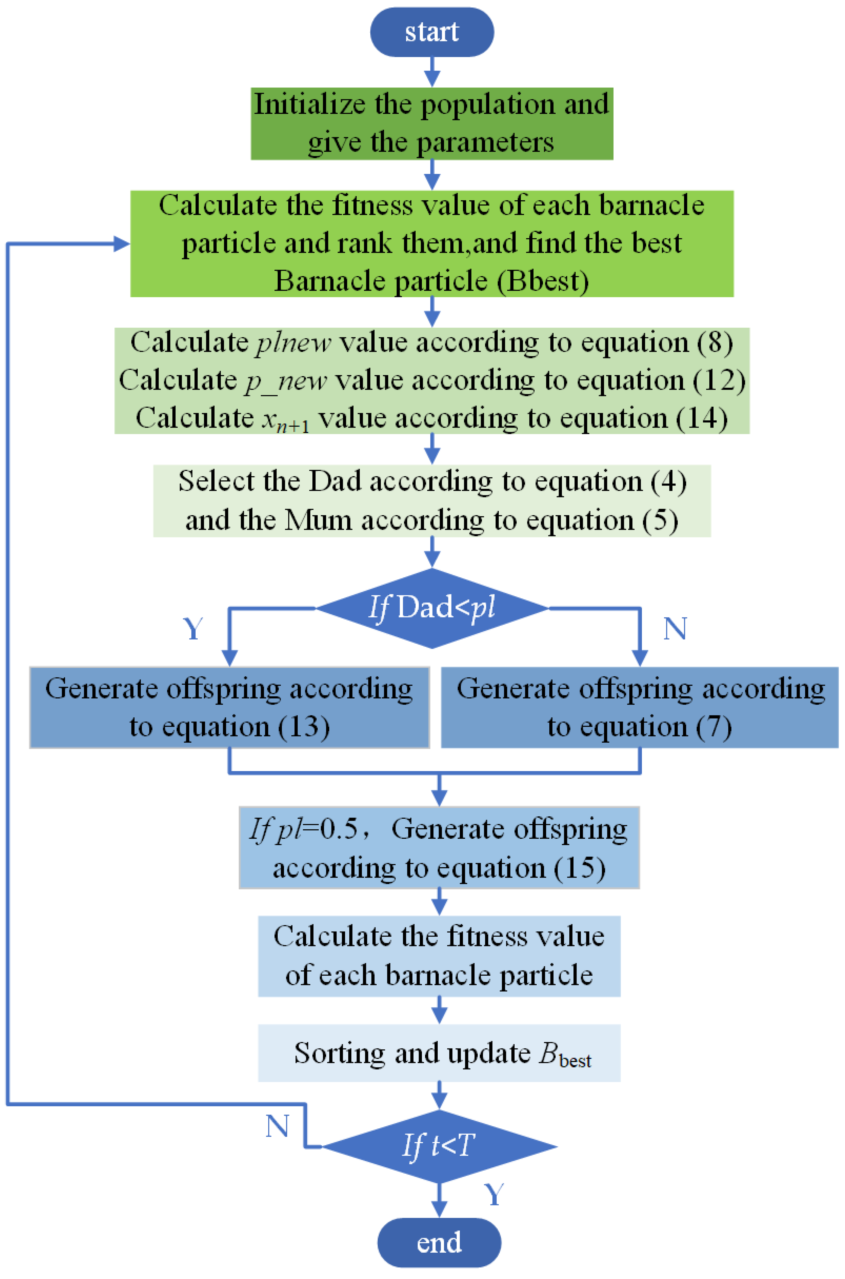
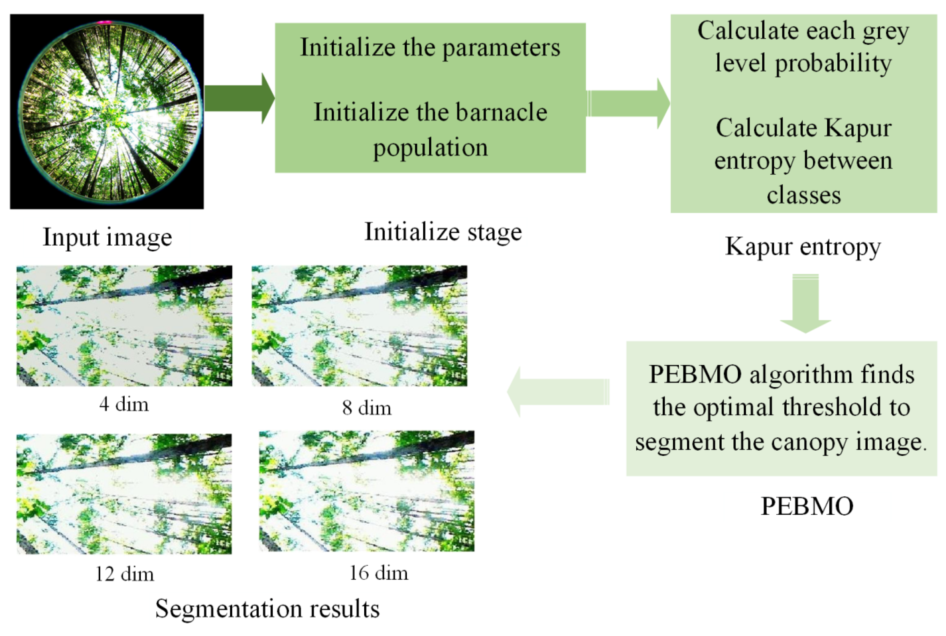

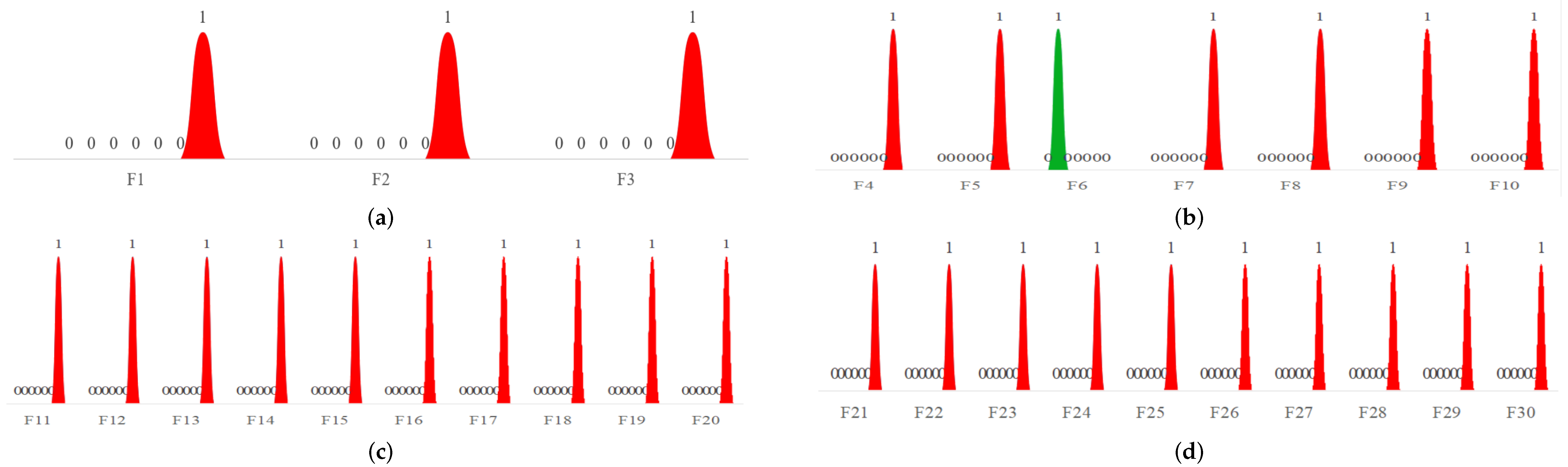
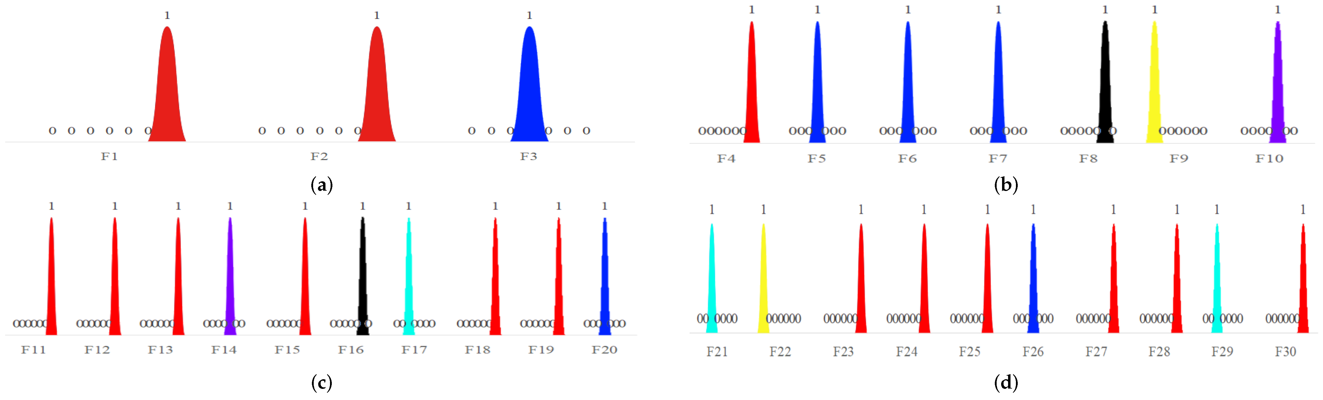
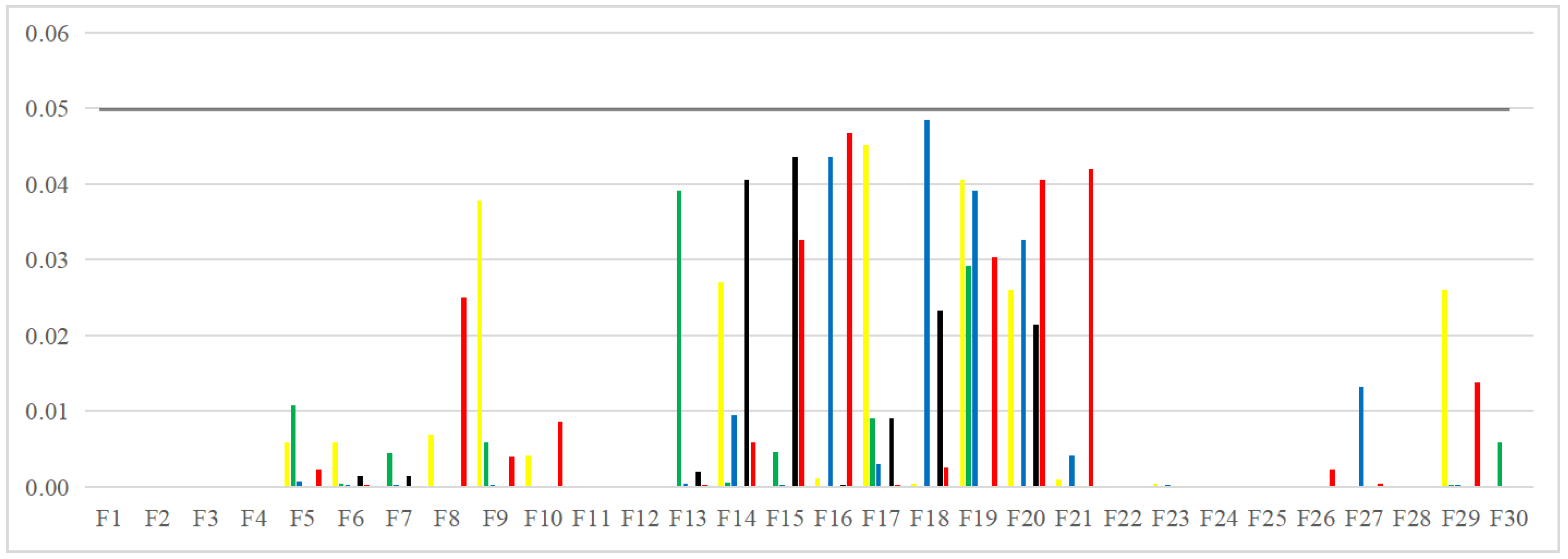
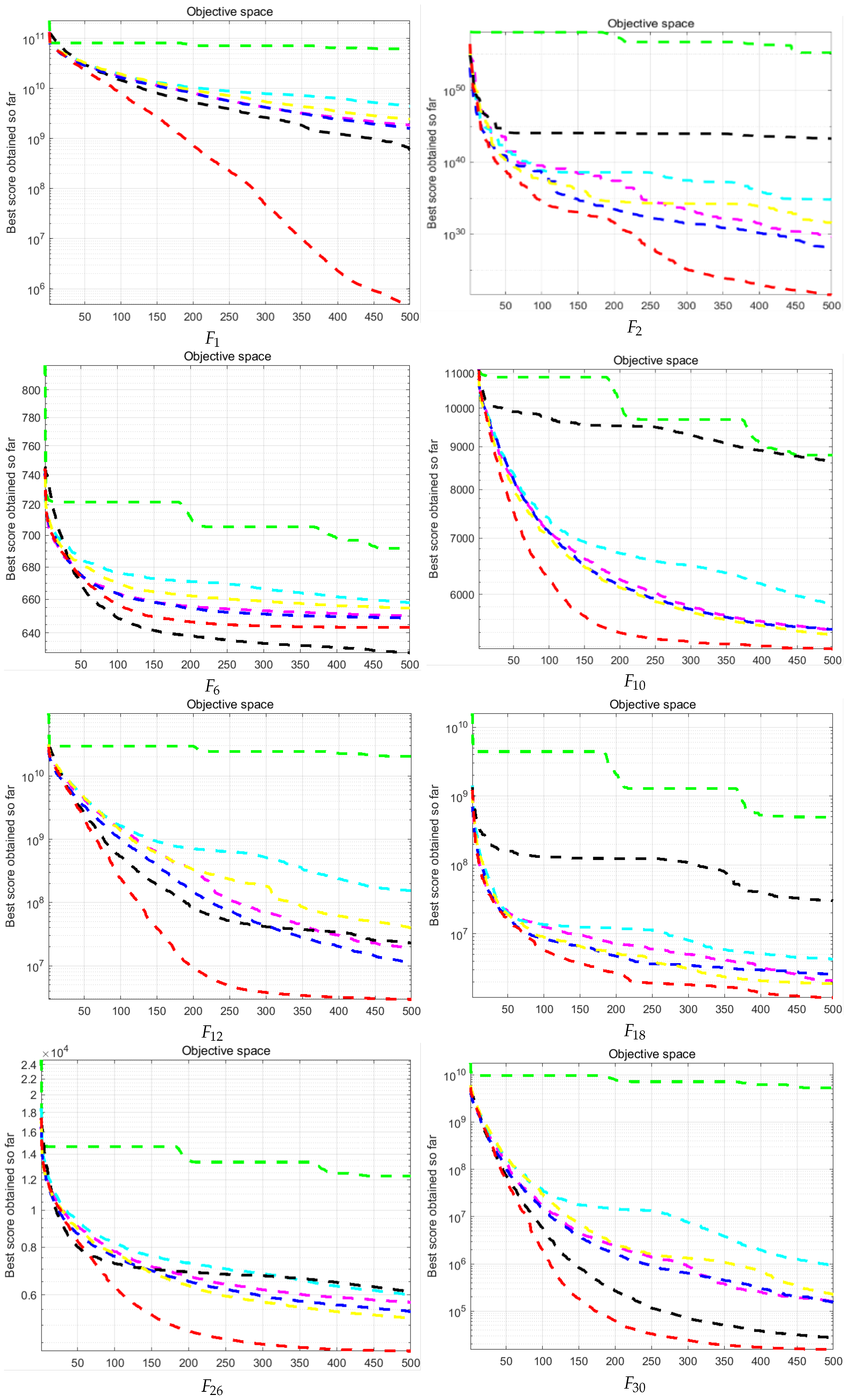
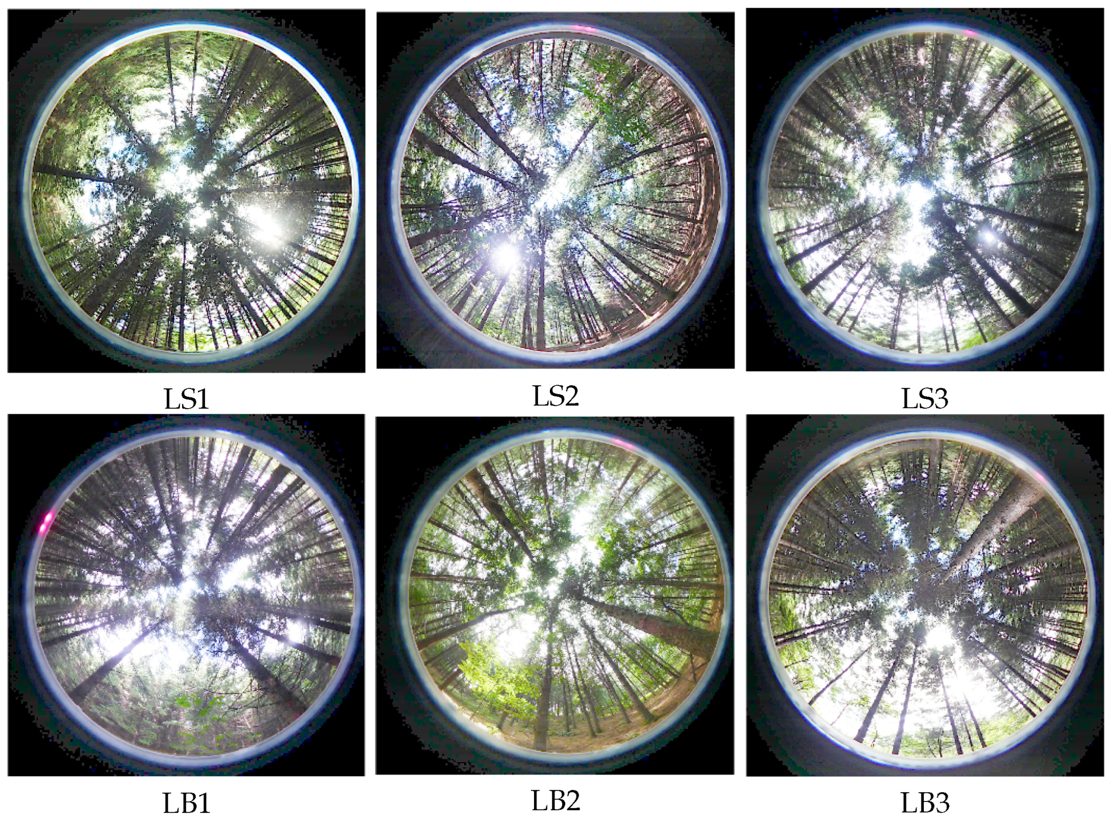
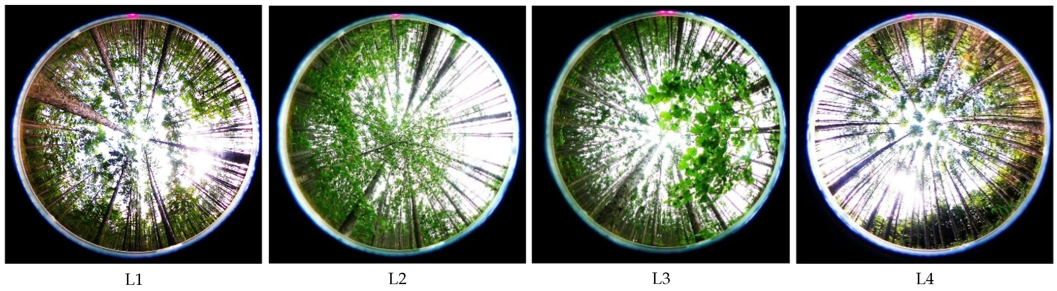
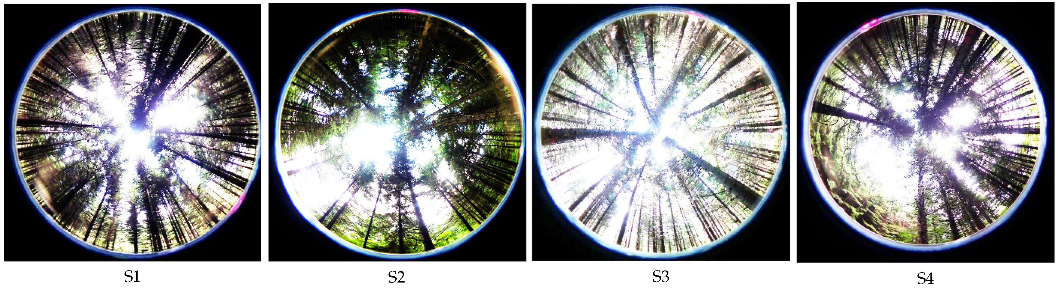
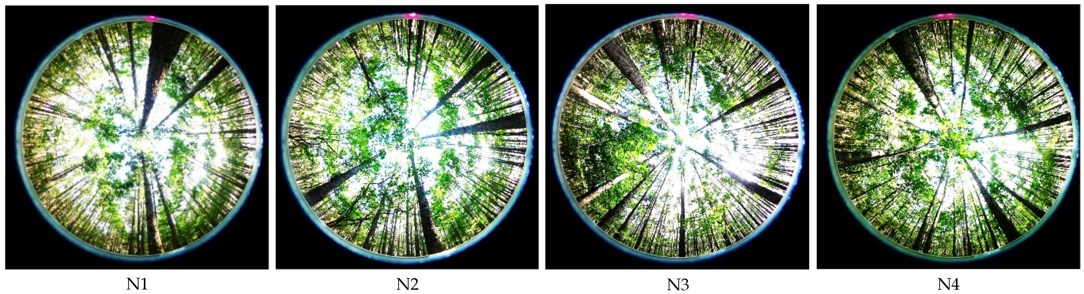
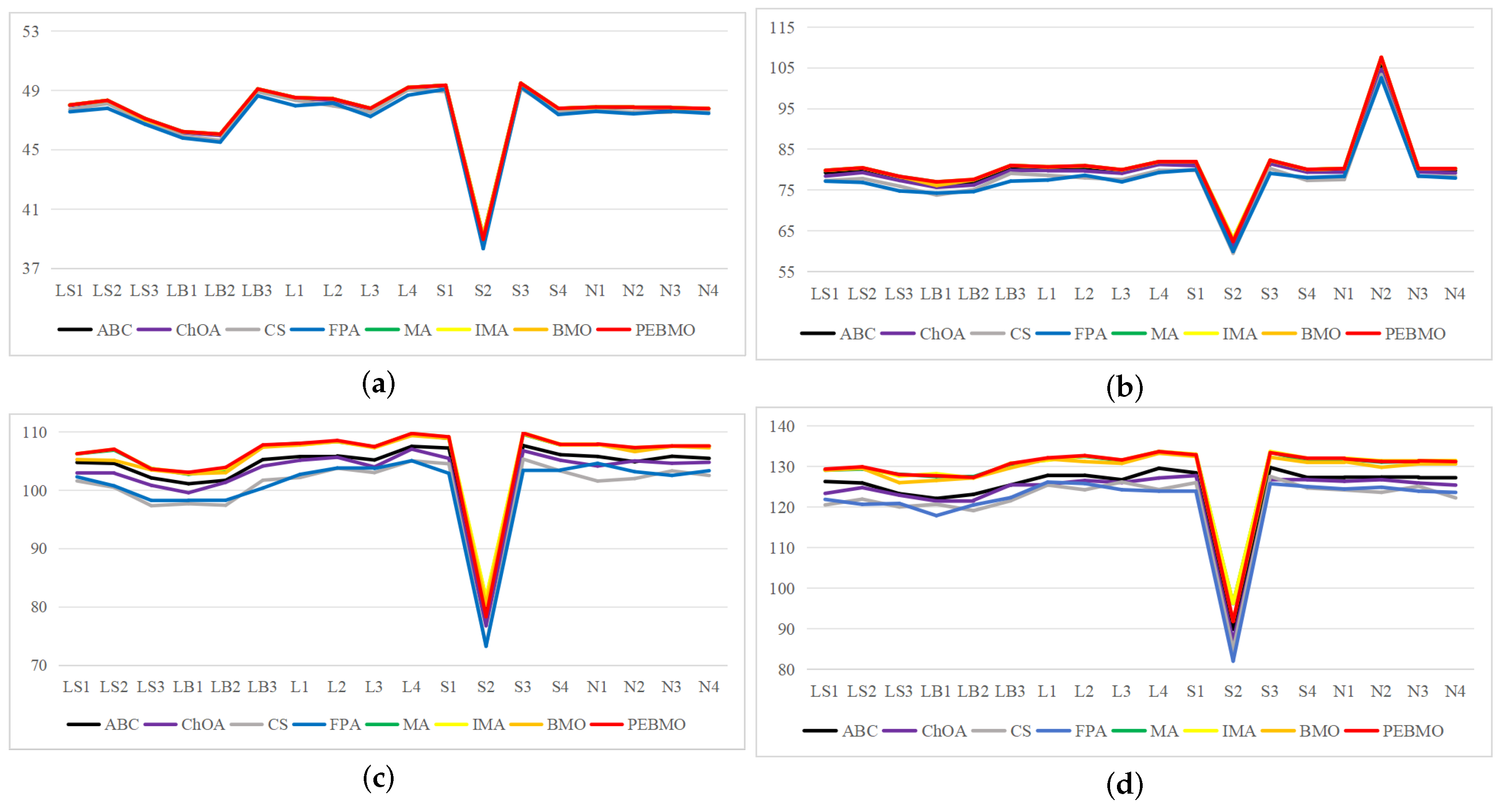
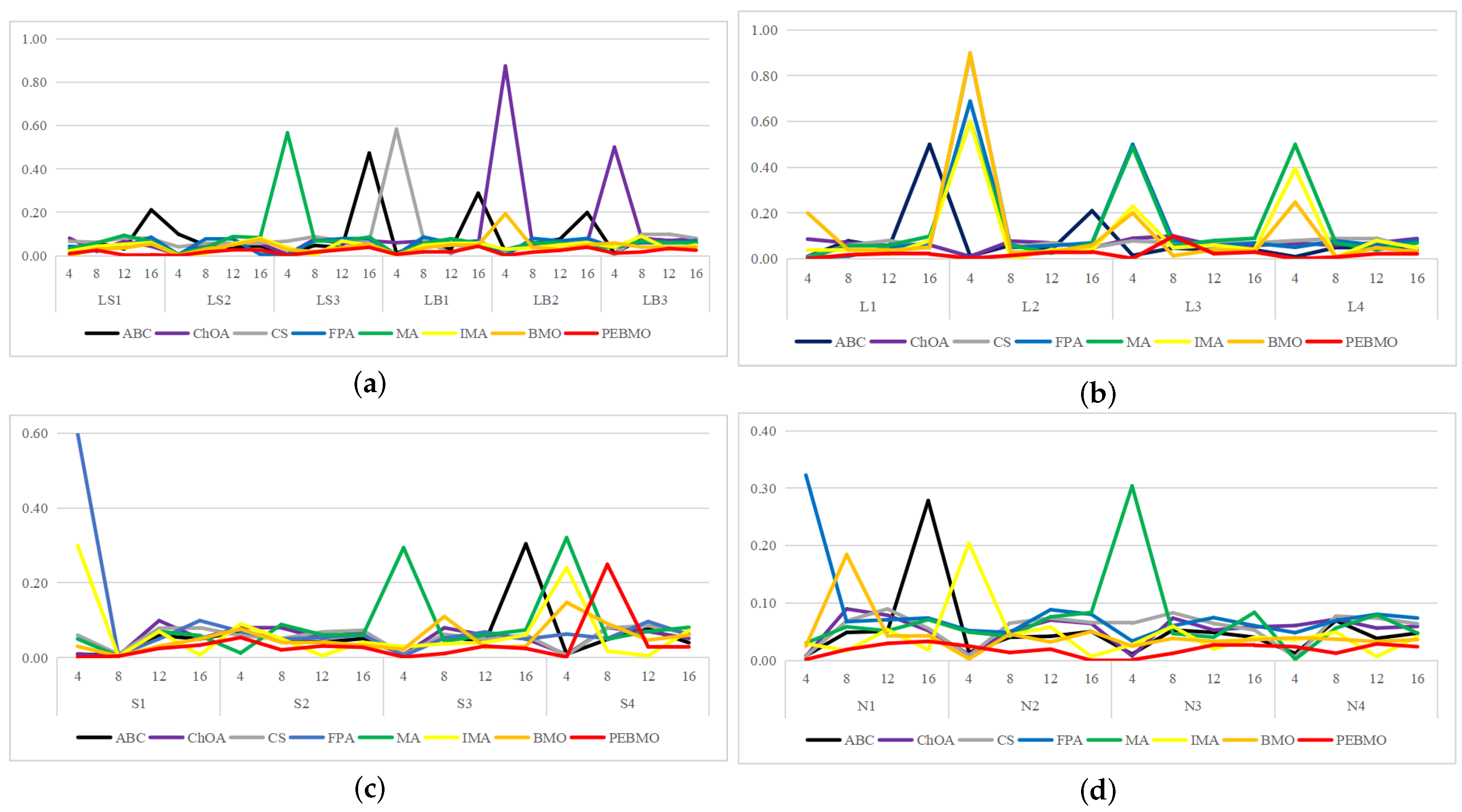

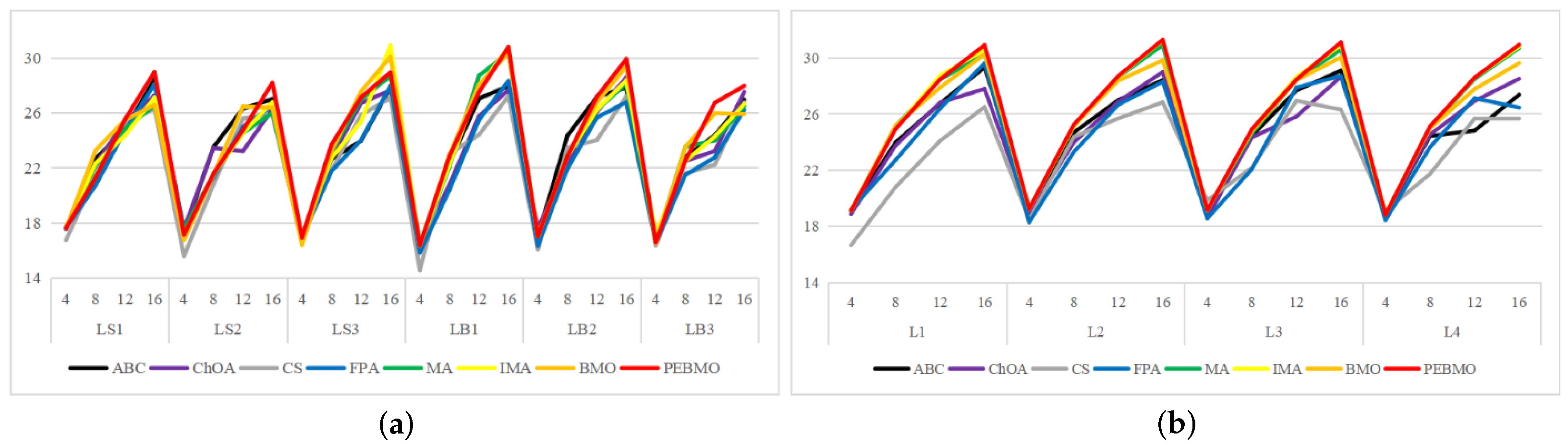
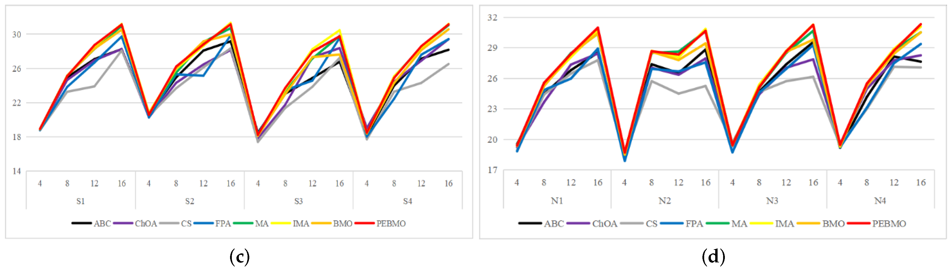
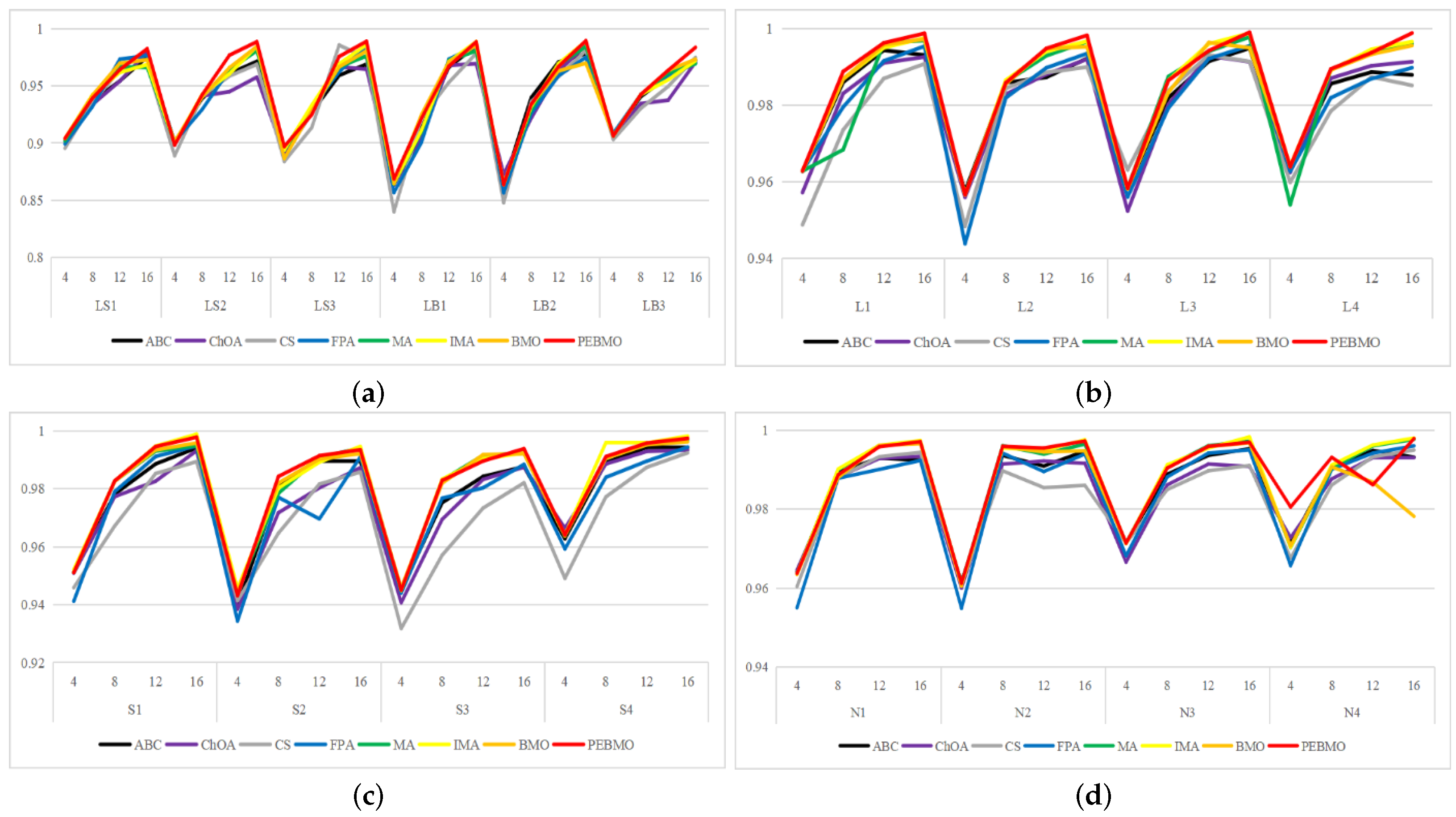
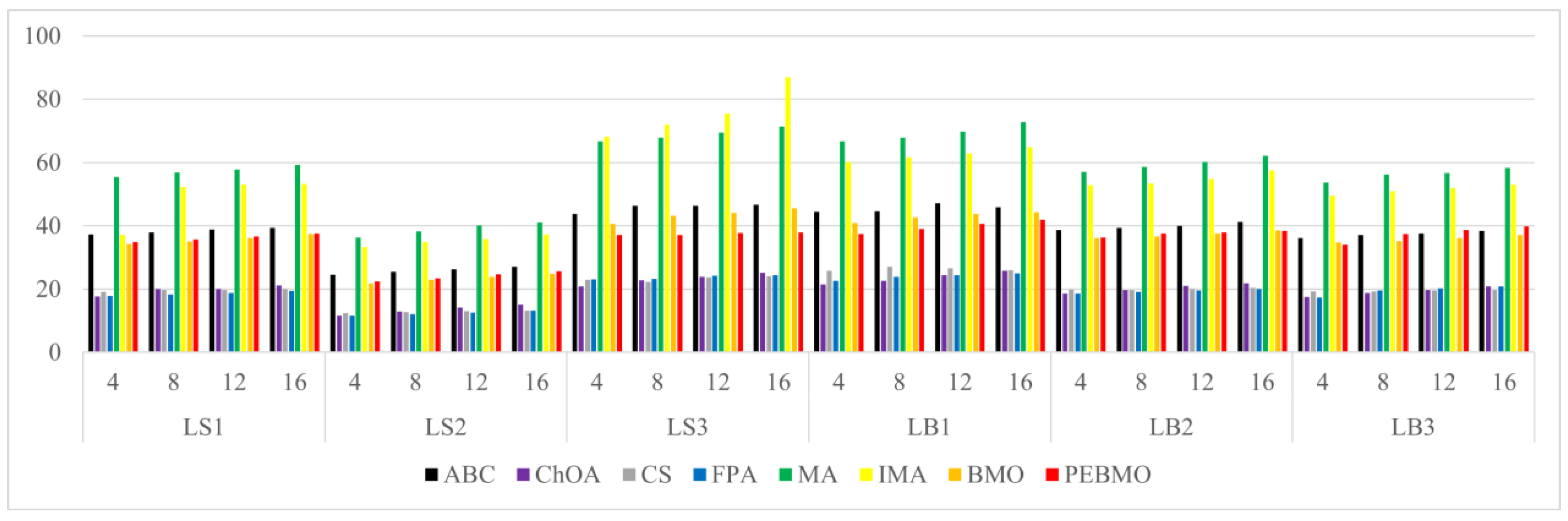
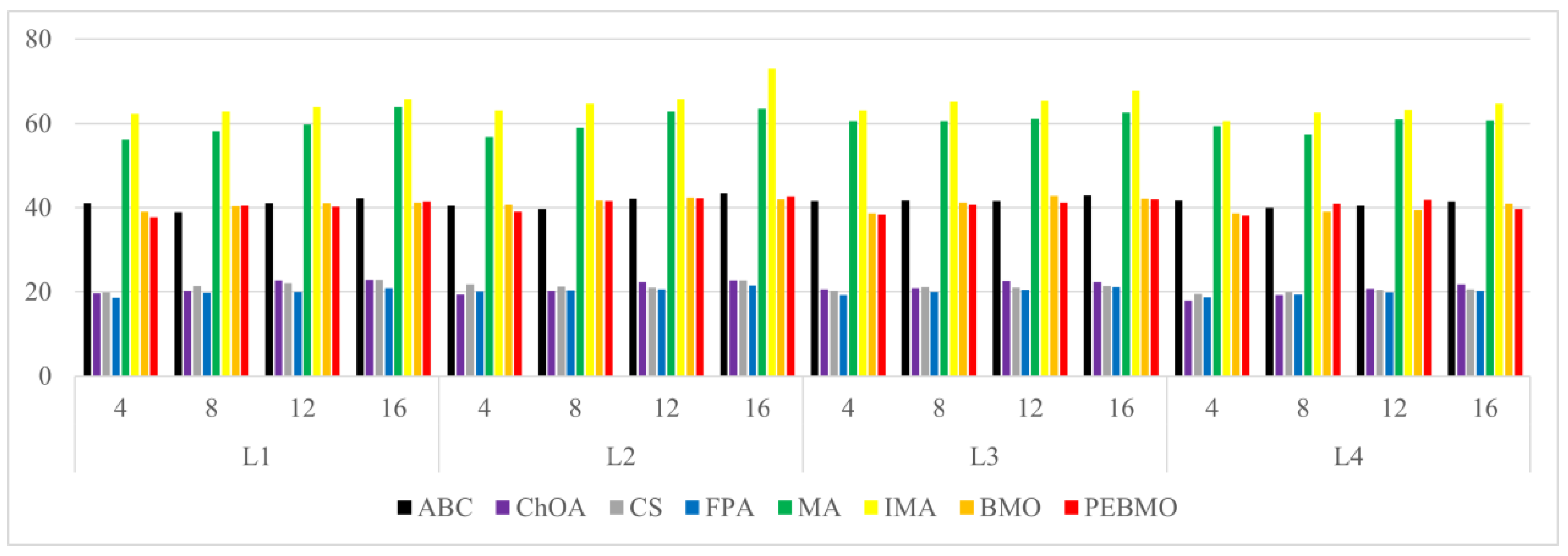
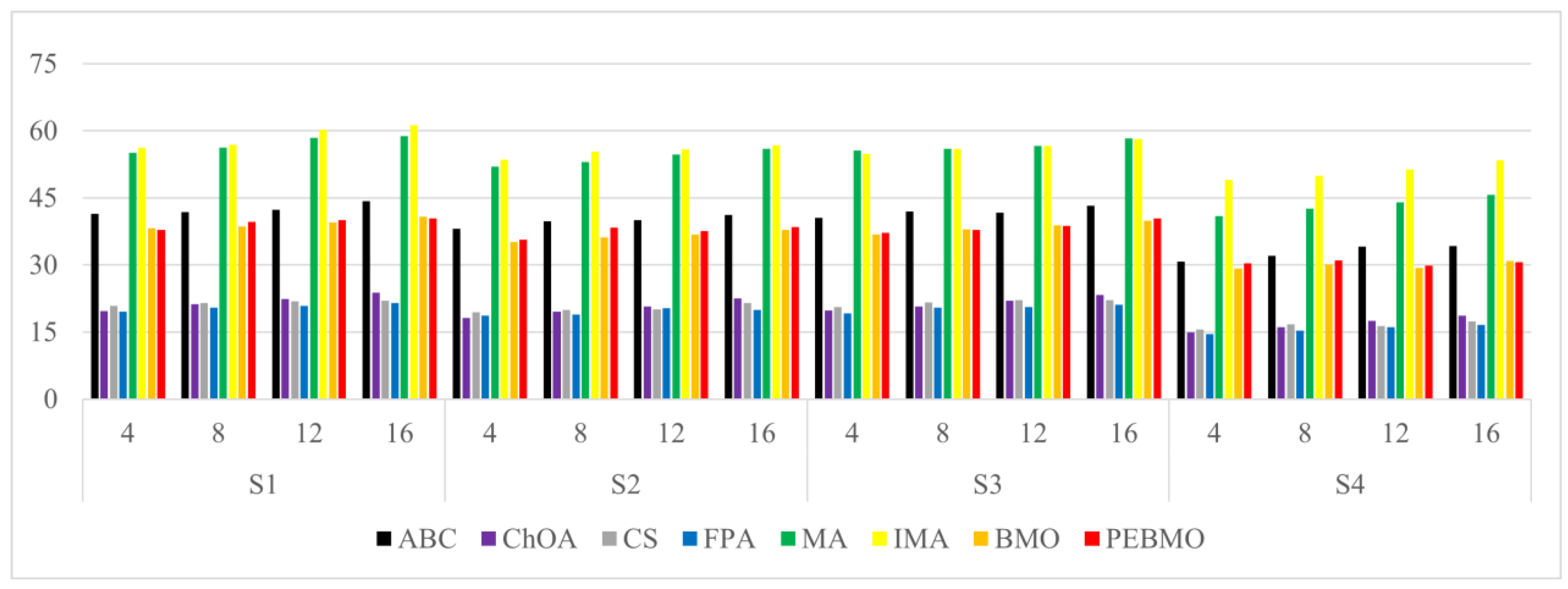
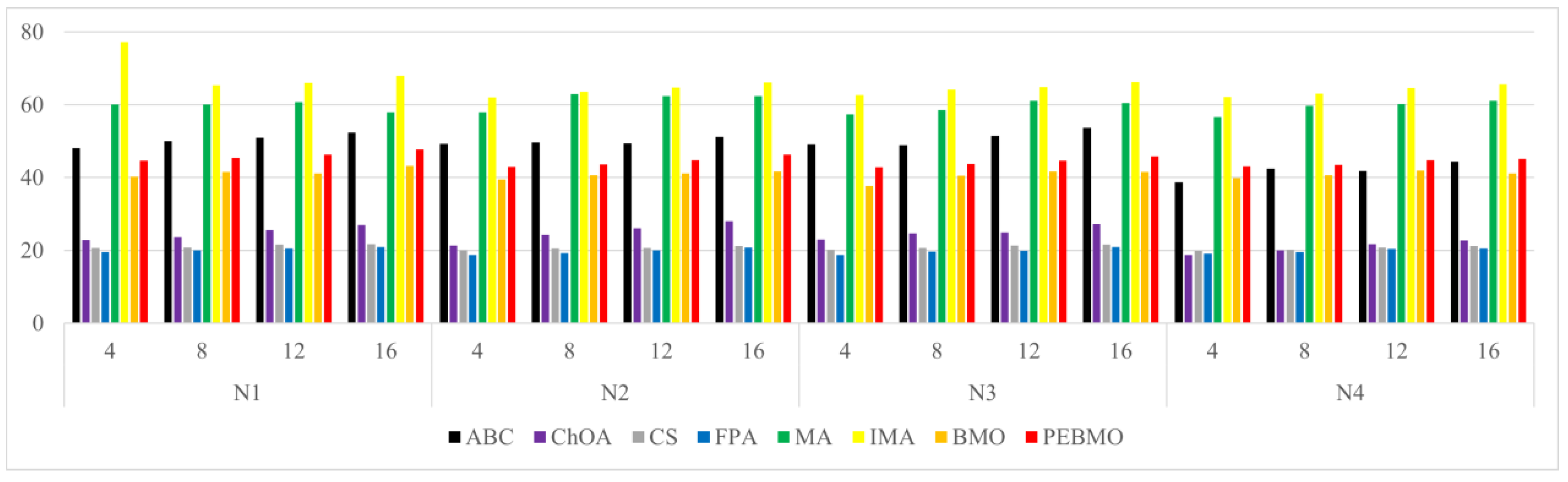
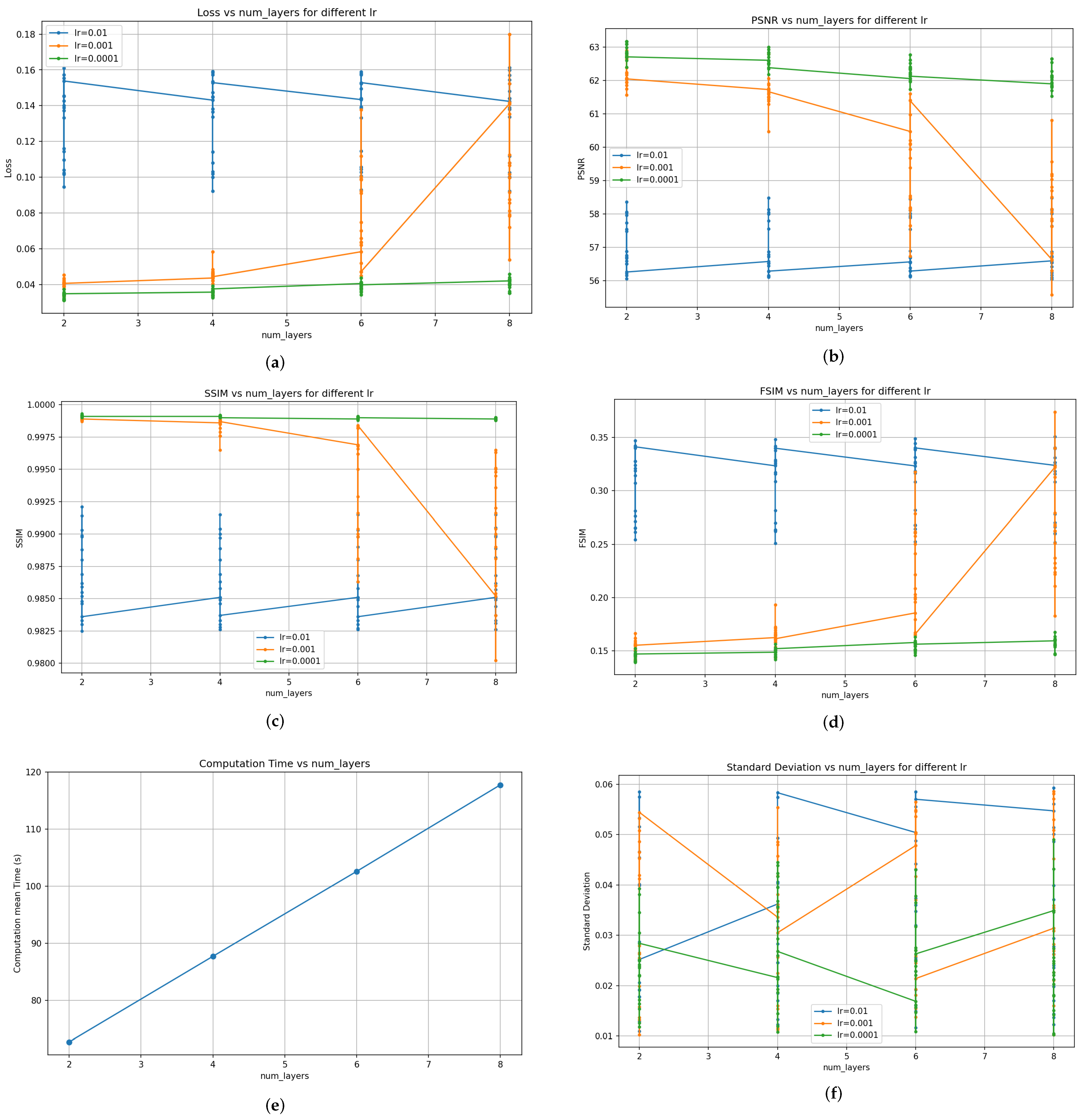
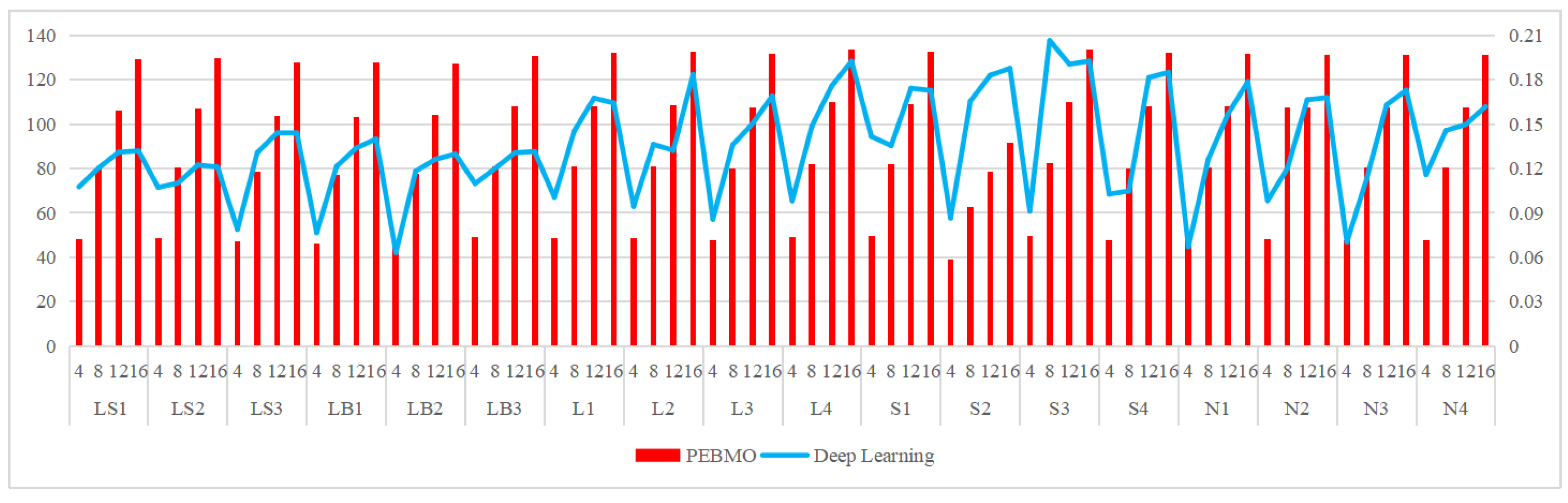
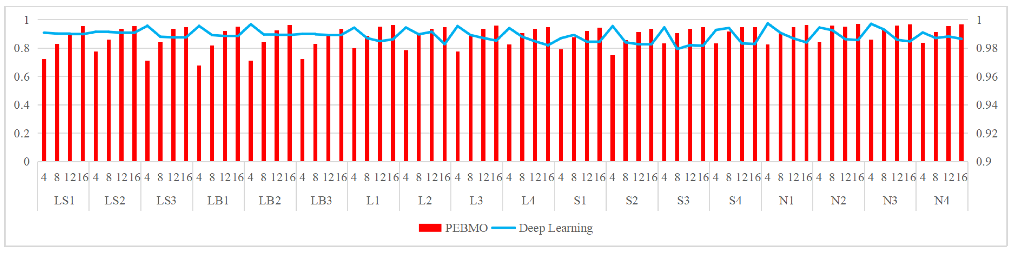
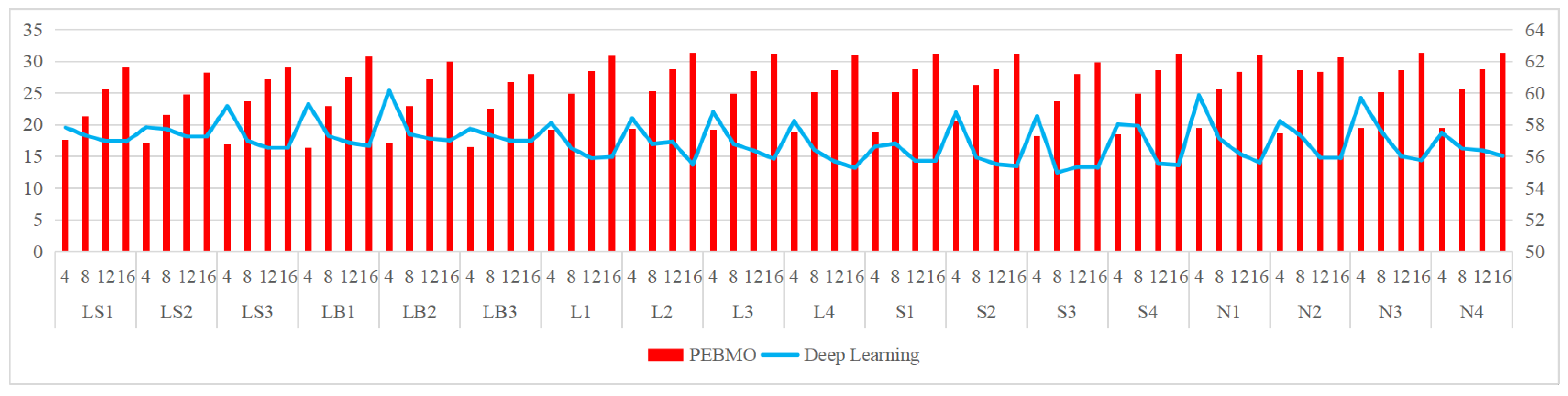
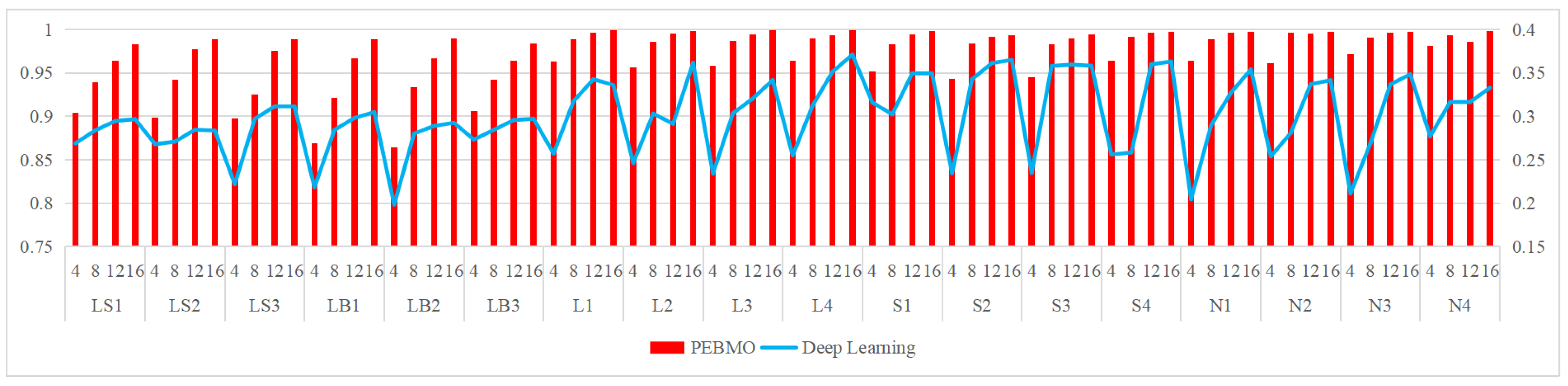
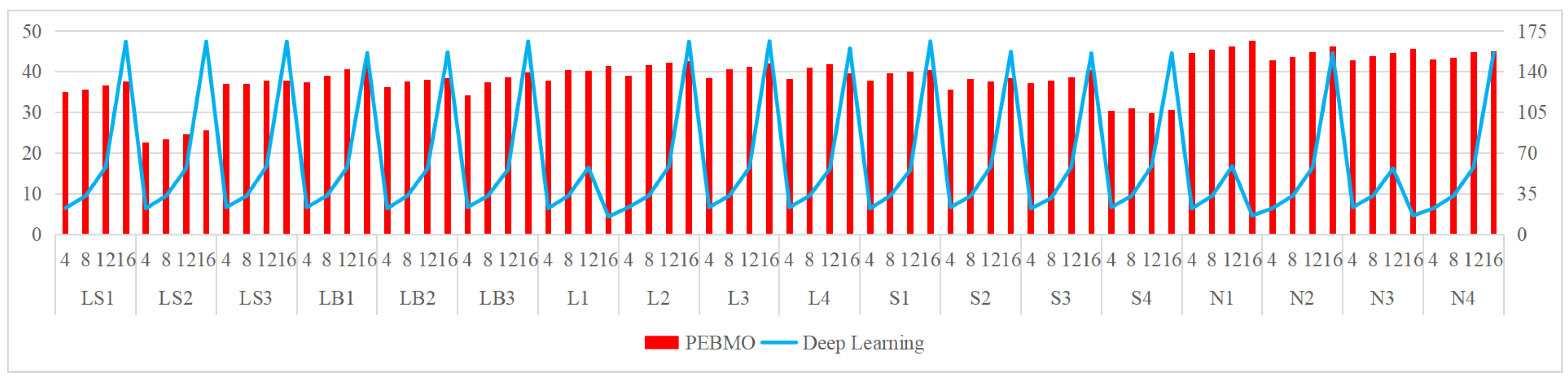
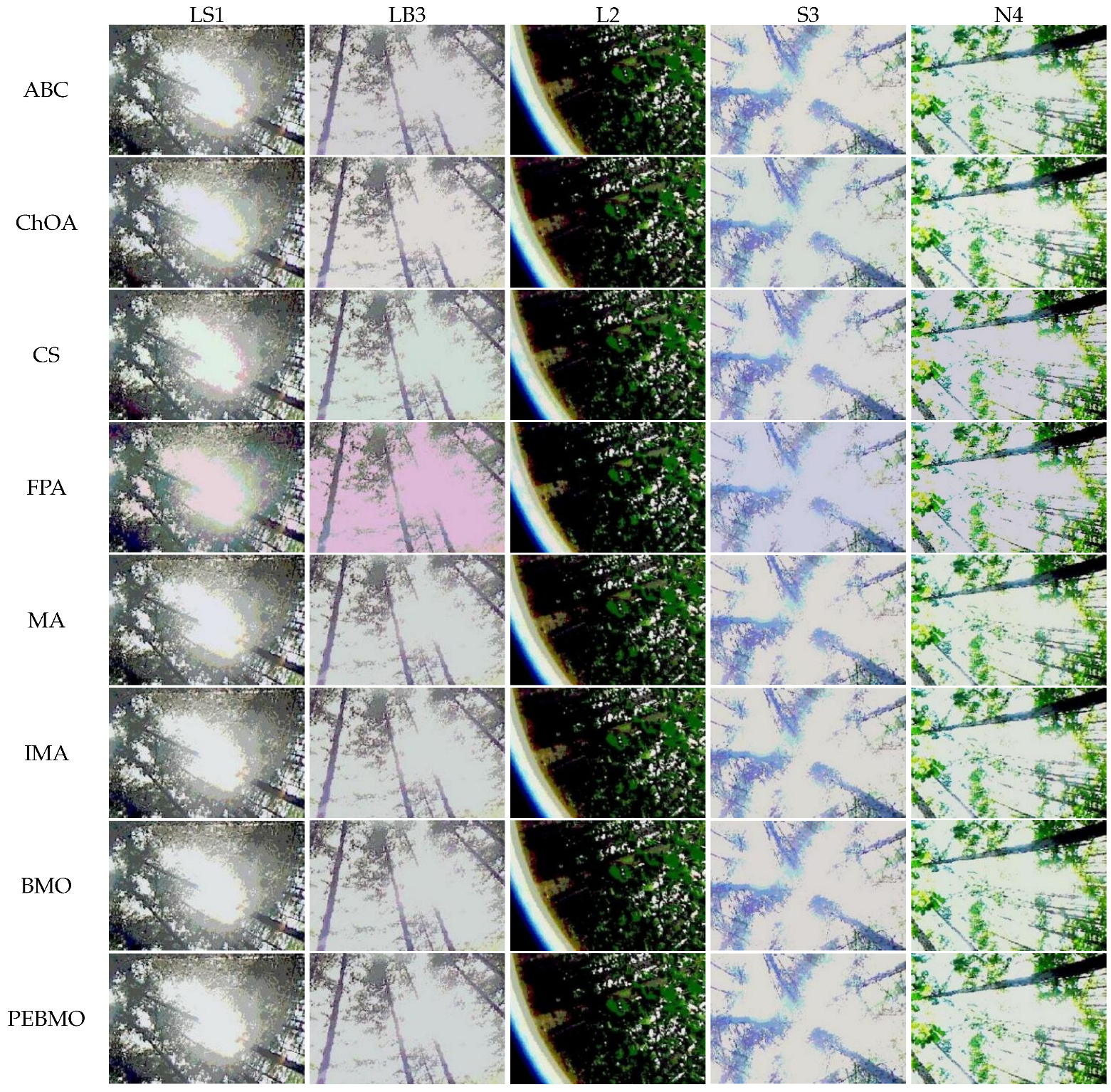
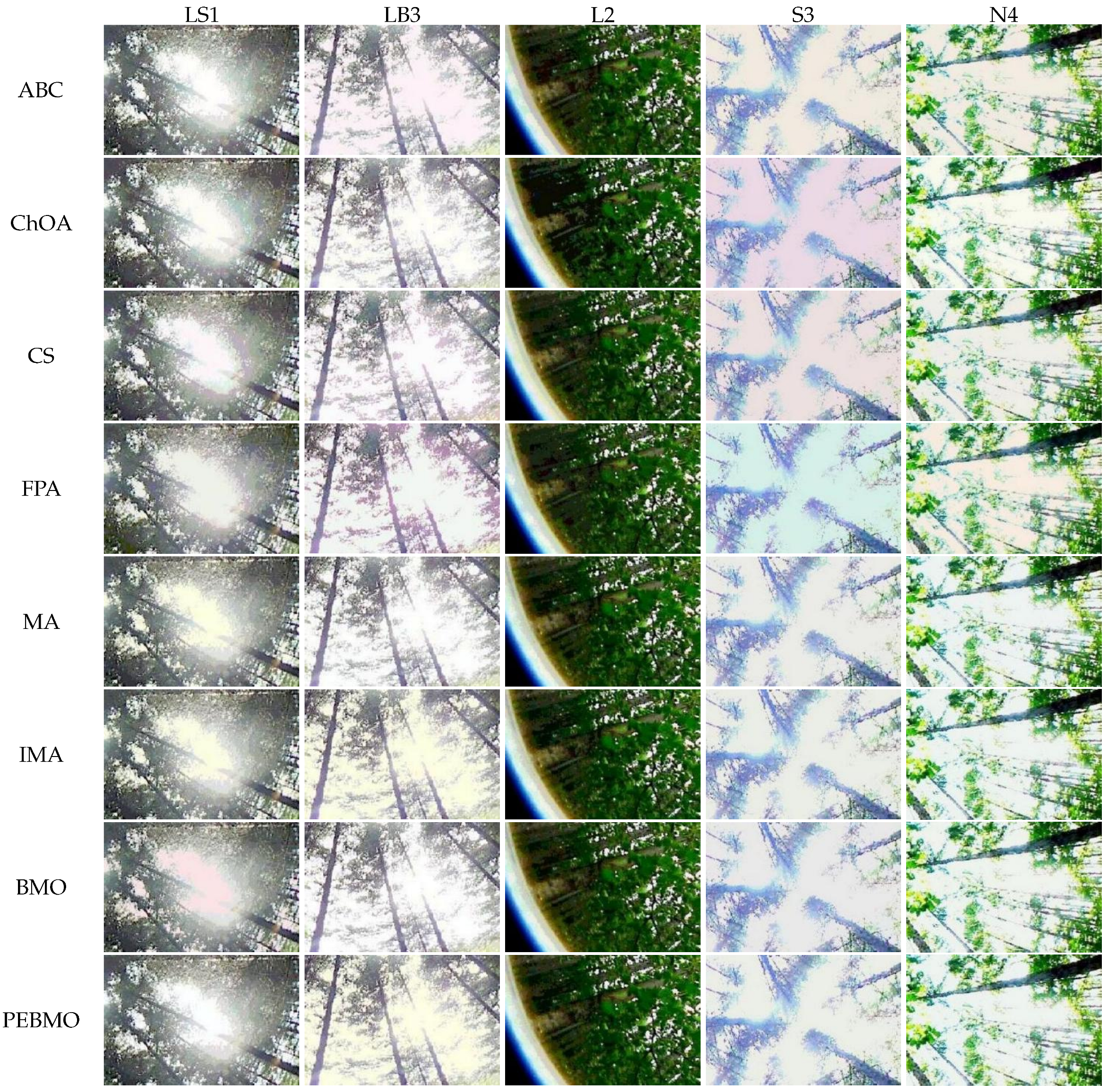
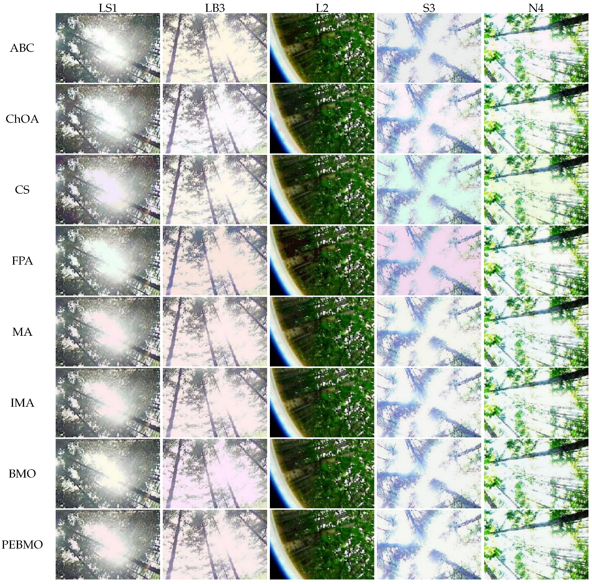
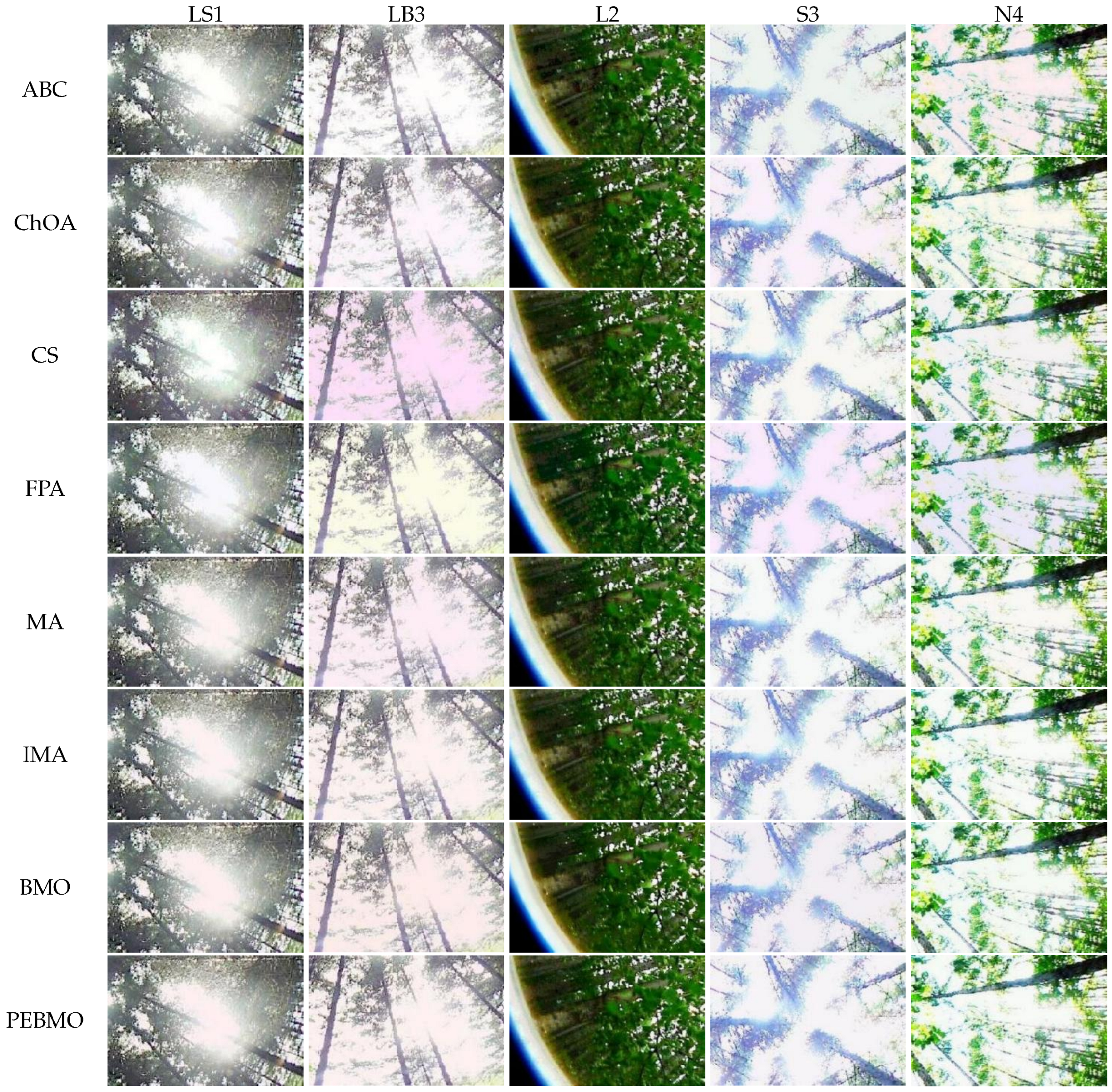
Disclaimer/Publisher’s Note: The statements, opinions and data contained in all publications are solely those of the individual author(s) and contributor(s) and not of MDPI and/or the editor(s). MDPI and/or the editor(s) disclaim responsibility for any injury to people or property resulting from any ideas, methods, instructions or products referred to in the content. |
© 2025 by the authors. Licensee MDPI, Basel, Switzerland. This article is an open access article distributed under the terms and conditions of the Creative Commons Attribution (CC BY) license (https://creativecommons.org/licenses/by/4.0/).