Resource Indexing and Querying in Large Connected Environments

Abstract

The proliferation of sensor and actuator devices in Internet of things (IoT) networks has garnered significant attention in recent years. However, the increasing number of IoT devices, and the corresponding resources, has introduced various challenges, particularly in indexing and querying. In essence, resource management has become more complex due to the non-uniform distribution of related devices and their limited capacity. Additionally, the diverse demands of users have further complicated resource indexing. This paper proposes a distributed resource indexing and querying algorithm for large connected environments, specifically designed to address the challenges posed by IoT networks. The algorithm considers both the limited device capacity and the non-uniform distribution of devices, acknowledging that devices cannot store information about the entire environment. Furthermore, it places special emphasis on uncovered zones, to reduce the response time of queries related to these areas. Moreover, the algorithm introduces different types of queries, to cater to various user needs, including fast queries and urgent queries suitable for different scenarios. The effectiveness of the proposed approach was evaluated through extensive experiments covering index creation, coverage, and query execution, yielding promising and insightful results.

1. Introduction

The IoT describes the network of sensors, software, and other technologies embedded in physical objects, “things”, to communicate and exchange data with other devices and systems. Nowadays, the number of IoT devices is increasing significantly. Sensors have become widely used in different domains and environments (e.g., agriculture 4.0, smart cities, smart buildings, smart grids, healthcare, and supply chains). According to [1], the number of IoT devices will reach 27 billion in 2025.

With such an increase in the number of IoT devices, collected data have grown in volume, and this will lead to the emergence of different problems, mainly related to resource discovery, privacy, and communication. In addition, resource querying has become a major issue, since queries must fit user needs, with a huge number of sensor nodes. In essence, various problems impact resource indexing and querying. Depending on the physical environment, some areas could have plenty of devices to cover them, while others would be partially covered or even empty (i.e., uncovered). This highly impacts the overall performance of the solution provided. Moreover, in many scenarios, different types of queries need to be handled to cope with the user needs. Some queries need an urgent answer, regardless of the cost. At the same time, others require precision and accuracy. Therefore, data querying in large connected environments needs a suitable and advanced indexing scheme.

In this paper, we propose a hybrid indexing approach in which resources (i.e., sensing devices) are indexed following a specific pattern that takes into account covered and uncovered zones. Following this pattern, devices will be able to receive and forward queries between each other directly. Our approach considers the limited capacities of devices to increase the network life cycle. In this paper, we extend a previous study [2] where global index generation was detailed. Here, we consider different complex scenarios, introduce the implementation of four types of queries along with experiments, and also explain the adopted architecture, as will be seen in the upcoming sections.

The rest of the paper is organized as follows. Section 2 presents a motivating scenario and highlights some needs and challenges. Section 3 details the categories of indexing approaches and presents related works, while showing their limitations. Section 4 defines preliminaries and assumptions. Then, we introduce the proposed indexing approach along with different querying techniques in Section 5. Section 6 presents the set of experiments conducted to validate our approach. The last section concludes this study and describes several future directions.

2. Motivating Scenario

In order to illustrate the motivation behind our proposal, let us consider the scenario of a connected wilderness open area. We suppose that a large number of IoT devices have been heterogeneously deployed in this area. This is a simplified example that illustrates the setup, needs, and challenges. Of course, it does not summarize all querying needs in a connected environment.

2.1. Connected Environment Setup

2.1.1. Environment Description

A connected wilderness open area has different landscape features: (i) lots of areas are highly accessible (e.g., plain fields), thus allowing easy sensor deployment and environment monitoring; (ii) a few areas are moderately accessible (like lakes and rivers), leading to challenging deployment and environment monitoring; and (iii) some areas are extremely inaccessible (e.g., rocky mountains and high surfaces) thus making deployment and monitoring highly difficult. As a result of the landscape setup, sensing device deployment is not homogeneous in the entire environment. Easily accessible areas (i.e., in open plains/fields) have a high node density, while moderately challenging areas (i.e., around water bodies) have a sparse node density. Finally, inaccessible areas contain isolated nodes in the best-case scenario or remain completely uncovered in some areas (i.e., no deployment of nodes) in the worst-case scenario.

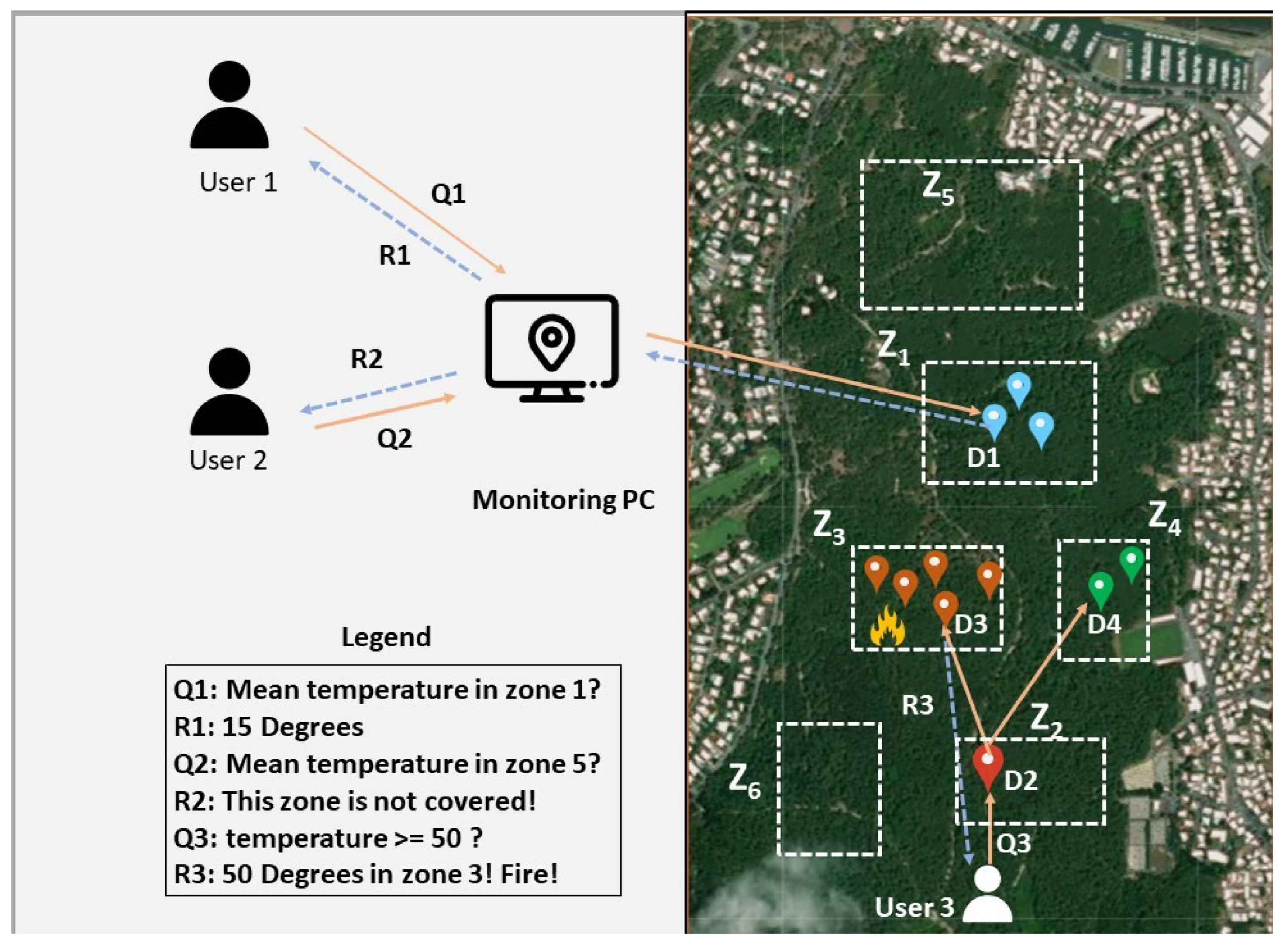
Figure 1 presents an example of a connected wilderness open area. This example shows the distribution of different temperature sensing devices in the Chiberta forest in Anglet, France. The objective of the deployment is to assess the potential for fires occurring within the forest. To distribute these sensors, a plane flew overhead and dropped the different devices, leading to a random distribution of the resources. This random distribution implies having areas with high sensor density, areas with low sensor density, and empty areas. Due to their restricted capacities, devices are unable to retain data about the entire network, which can pose significant difficulties in forwarding messages to the zone targeted by the query.

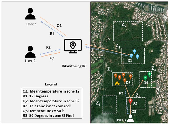
Figure 1. Environmental monitoring in the Chiberta Forest.

We also assume that the network should handle different types of queries, based on the needs of the user (urgency levels). To send a query, users can send a query from a monitoring PC by indicating on the screen the zone desired or by specifying GPS coordinates. Then, the monitoring PC will transfer the query to the appropriate device. Furthermore, users have the choice to directly send queries to the nearest device, which will then handle the request. Let us take some examples to illustrate the sending of queries:

• When a supervisor (user 1 in Figure 1) would like to know the temperature of a zone, she/he draws visually on the monitoring PC the zone to be requested. The PC sends the request (Q1) to the zone’s head (D1) located in or near the targeted zone. The respective device will return a response with the temperature of the zone.
• Another agent (user 2 in Figure 1) wants to gather the temperature of another zone (Z5). He draws visually on the monitoring PC the requested zone, and the query is forwarded to the nearest device. If the device knows from its own index that the requested zone (Z5) is uncovered, it can return an immediate response without further forwards of the request, consequently avoiding the usage of other devices’ capacities.
• Another interesting case is when a firefighter (user 3 in Figure 1) is trying to put out a fire but does not know its exact location inside a large and dense forest, in which fire can spread rapidly. The firefighter seeks to take out affected regions by activating the fire suppression system to extinguish the fire before it can progress further into the forest. He must predict the fire progression to activate the system in specific areas instead of activating it in the entire forest. The request is based on exceeding a certain threshold, indicating that a fire is probable. In the forest, he/she needs to urgently broadcast a request in order to quickly retrieve the fire’s location. After broadcasting the request, one or several devices will be aware if a fire is detected within their zones (e.g., zone 3). The response is sent back by at least one of those devices.

The response can contain the data queried, but it can also be a label indicating that no response could be received (uncovered zone due to the uneven distribution of the devices). To send a response, the device can either forward the response directly to the user or retake the query path to return to the sender.

2.1.2. Device Properties

Sensing devices are deployed in the wilderness and need to function autonomously. They rely on their resources to sense observations from the real world, process data (when possible), and exchange/communicate with each other using a wireless network. Although these sensors have different storage capacities, few of them are capable of storing resource index information about the entire environment. Of course, devices can have many sensors (gas sensors, infra-red sensors). Here, for the sake of simplicity, we will only focus on temperature devices with the necessary protocols that allows them to communicate between each other.

2.1.3. Data Retrieval

Members of the environmental team need to retrieve data from any sensing device or zone. They can retrieve data directly from the device (when they know its identifier). However, sometimes this is not possible, and queries need to be sent to a zone (without knowing who is in charge of managing it). Devices must be able to forward a given query in case the current zone is not the corresponding requested zone. When the latter is uncovered, the device will be able to return an explicit response (noting that it is an uncovered zone, i.e., a zone without a device). Moreover, to comply with different querying needs, several query types exist. For instance, a user needs to quickly retrieve the temperature from any device covering a targeted zone, while another user wants to be sure that no fire is detected within another specific zone. If a quick response is needed, she can execute a low priority query call. In another case, the user wants to detect that there is a probability that a fire could happen. Then, a high-priority query must be sent. Finally, the user may want to send a query with a moderate priority to test the temperature for experiments. During the querying process, a query may take some significant time to respond (such as high priority queries), while others can return a response quickly (such as queries with a low-level priority). Queries having a moderate urgency will return a response with a time between low-level and high-level queries. We note that we will define the different levels of query urgency in the upcoming sections.

2.2. Needs & Challenges

This scenario shows several needs to be considered:

• Need 1—Query types: users need to detect events, while considering different urgency levels (e.g., a wildfire is more urgent than requesting information for data analytics) in their queries;
• Need 2—Device capacity-based querying: users needs to send their queries to optimal (indexed) devices in a way that reduces network usage and provides the best possible response;
• Need 3—Location-based querying: users need to issue a query from any place in the environment. They also need to retrieve data from a specified area/zone (e.g., obtain temperature data from the left side of the forest), from an unspecified area/zone, i.e., based on a target objective (e.g., obtain alarming high-temperature readings), or based on a combination of both (e.g., obtain alarming high temperature readings from the left side of the forest).

However, as presented in Figure 1, some issues might affect the aforementioned data retrieval queries: (i) IoT devices cannot store the entire environment’s information, since they have limited capacity, in addition to the vastness of the environments; (ii) different deployment densities and coverage issues make spatial querying more complex. Some zones may be covered by devices, while others might not; and (iii) depending on the user’s request, the user may require a response at all costs, consuming high resources due to the importance level of the query. To manage the aforementioned issues, different challenges should be addressed:

• Challenge 1: How to consider the capacity of the devices in each index, in order to optimize network lifecycle and querying?
• Challenge 2: How to maximize the index’s coverage by considering covered and uncovered zones?
• Challenge 3: How to adapt the indexing scheme to the different types of queries?

3. Related Work

3.1. Indexing Overview

To collect data, sensor and actuator networks are critical components of the IoT architecture. In addition, the number of connected nodes has expanded in recent years, generating a tremendous volume of data. The goal of an indexing scheme in a connected environment is to quickly find and retrieve a resource that contains the desired data from a group of linked devices. According to Y. Fathy et al. [3], indexing can be classified into three categories in connected environments: data indexing, resource indexing, and indexing of higher-level abstractions. Data indexing refers to organizing IoT data (e.g., sensor measurement/observation) to enable fast search and retrieval of the data, without identifying the data source. Resource indexing refers to organizing IoT resources (e.g., sensor, service, device) to facilitate querying or finding a specific resource or a resource that can answer user queries. Finally, data abstraction is a transformation of lower-level raw data (e.g., 2 °C) into higher-level information that describes patterns or events (e.g., cold weather). Higher-level abstractions refer to inferring information and insights from published raw data using various IoT resources, such as events, activities, and patterns.

In this study, we focus on resource indexing, which can be divided in turn into three categories: spatial, multi-dimensional, and semantic indexing. Spatial indexing uses geographical features like latitude, longitude, and altitude coordinates to represent the environment component scheme (e.g., kd-tree, R-tree, geohashes…). Multidimensional indexing [4,5,6] treats resources as multi-feature objects and aims at simplifying mapping/identification IoT resources (to unique identifiers). Semantic indexing [7,8] relies on the enriched (semantic) description of IoT resources.

Much research has been conducted on resource indexing. Mohamed Y Elmahi et al. [9] showed a survey in which resource discovery techniques were classified into different categories: (i) protocol-based, in which protocols are used to find the appropriate device, such as CoAP [10,11], SSDP [12], TRENDY [13], and DNSNA [14], which mainly rely on the domain name system DNS; (ii) architecture-based, where different architectures were discussed, such as centralized [15], distributed [16], and hybrid [17]; (iii) semantic approaches, where devices are represented and grouped depending on their knowledge, such as in [18,19]; (iv) location-based, which focuses on the device discovery in a local area, such as in [20] (smart homes for example), or a remote area for larger environments, such as in [21]; and (v) clustering-based, which builds communities or groups by connecting and linking resources, such as in [22,23].

In this paper, we focus our literature review solely on spatial indexing, since our approach falls into this category, as our resources here are not multi-dimensional and do not embed semantic features. Following the classification schema of [9], we can classify our approach as an architecture-based discovery technique, since a distributed design is adopted. It can also be allocated to the location-based indexing approaches, because it relies on a spatial indexing technique that requires the resource location. In what follows, we present research studies belonging to the spatial resource indexing category.

3.2. Indexing Approaches

In [24], the authors built an indexing tree to access different resources. The algorithm relied on hashing a key k into geographical coordinates. Each node contained a key-value accessible by users when queried. An extension of their GHT algorithm is the DIFS [25] approach, where non-root nodes may have more than one parent. When a query is requested, it starts with nodes that cover exactly the query range, then it will go down the index until it reaches a node that covers the entire network and having the value requested by the query. These algorithms use a data-centric architecture, which means that the device capacities are not considered. Plus, they consider the spatial intent of the network without having information about uncovered zones.

Similarly, a quadtree indexing technique was presented in [26]. The authors proposed a spatial approach named GH-indexing, in which the divide and conquer approach was used to build a distributed quadtree by encoding the locations of loT resources into geohashes and then building a quadtree on the minimum bounding box of the geohash representations, with the root node representing the whole spatial range. Starting at the root, the algorithm, in order to discover IoT resources, evaluates each child node and tests if its minimum bounding rectangle intersects with the region being queried. A list of geohashes that intersect with the query minimum bounding rectangle is returned. In this paper, the authors did not take into consideration that zones might be uncovered. Cases where devices could be far away from the queried region will give inaccurate results. In that case, this region should be considered uncovered. Plus, since data are stored in a repository, the device capacities have no importance in this case.

Similarly, Fathy et al. [27] introduced an indexing technique that leveraged a modified version of the DP-means algorithm. DP-means is a clustering algorithm where a new cluster is created when the distance between data points exceeds a threshold. $\lambda$ is initialized as the standard deviation of the data points (resource locations). Then, the sensors are clustered into different clusters. They also proposed an architecture where each gateway is responsible for forwarding queries to a cluster of sensors. A discovery service layer is responsible for forwarding the queries to the appropriate gateway. After receiving a query, the discovery services forward the query to the gateway having the smallest distance between its centroid and the query and having the type of data requested. Since this method clusters different devices, the queries concern only zones(specific locations) having at least one device. Queries are also considered one-path queries, since the query follows a unique path and the request may or may not return a result. In this case, different query urgency types were not implemented. Thus, important/guaranteed data could not be collected.

J. Tang and Z. Zhou in [28,29] showed tree indexing techniques, while preserving energy principles. They presented two algorithms (ECH and EGF-Tree) where the area is divided into sub-regions based on grid division, to mitigate the energy consumption in a network of energy-limited sensors. These regions are clustered following the energy minimum principle. After generating the tree, sensors report their data to the base station. They also proposed a query aggregation plan: the query is routed from the root node to the leaf using the EGF tree until the desired leaf nodes are reached. Sub-query results are returned to the base station using in-network aggregation. The result of the query is derived from the results of the sub-queries. The authors specified that devices are distributed unevenly to different areas, but they did not consider that an uneven distribution may lead to zones with no devices. In other words, uncovered zone manipulation was not specified in their case.

In [30], the authors proposed an architecture for indexing distributed IoT sources, where different discovery services are connected using Gaussian mixture models. Gaussian mixture models are used to represent a normally distributed population in an overall population. Traditional indexes are replaced by a mathematical representation of the distribution of IoT source attributes. This approach (DSIS) relies on probabilistic indexing to determine which discovery server or gateway the query must be forwarded to. Going down through the proposed structure, the aggregated models become less sensitive to probability. The search algorithm ends when it finds the source or reaches the maximum number of permitted hops. In addition, they proposed an updating mechanism with small and large intervals. Here, capacities are defined as the number of sensors for a WSN. The data points are updated following an updating mechanism using temporal or complete updates. The queries defined in this approach are queries considered guaranteed, since, in case of a failure, a recovery process is applied from an upper level of the architecture until trying all possible paths. These type of queries will return a response at all costs but may consume a lot of resources.

In [31], a tree structure called BCCF-tree was proposed having two principle layers: an internal node level (nodes that contain two pivots and two pointers and are stored in a fog computing layer) and a leaf node level (nodes contain containers and stored in cloud computing layer). The proposed indexing approach is to create clusters by determining the distance r between two pivots, then determining the distance between one of these pivots and the centroid of existing clusters (created using k-means), such that this distance is less than r. This process is repeated until an indexing tree is formed. When a user issues a query, the search starts between the query point and the pivots when going down the tree. The distance between the pivots and the query point shrinks while going down. The environment is divided following resource similarities inside the environment. The authors defined the capacity as the maximum number of sensors a container can accommodate. Since the query is forwarded to the appropriate resource as the radius shrinks, queries are considered one-path queries.

C. Dong et al. [32] proposed an IoT index method named A-DBSCAN, which consists of clustering sensors using DBSCAN. DBSCAN is a famous density-based algorithm that groups data points that are close to each other. This can result in forming large-sized clusters. The same clusters will be clustered again using K-means to simplify and reduce the form of these clusters. Users can start sending queries to these clusters. In addition, in the user search method, users can send feedback on the obtained responses. Based on this feedback, the responses are updated for the next queries. Since this algorithm depends on users’ feedback and directly forwards the query to the device, the queries can be considered fast. The device capacity is not considered, since this is a centralized architecture and these criteria have no importance in this type of architecture. Moreover, this algorithm does not consider that zones may be uncovered.

3.3. Summary Table

In Table 1, we present a comparison between the different approaches based on three criteria.

Table 1. Comparison table of indexing approaches for IoT resources.

	Device Capacities	Types of Queries	Indexing Coverage
GHT/DIFS [24,25]	No	One-path	Only Covered zones
GH-Indexing [26]	No	One-path	Not explained
Mod. DP-means [27]	No	Sequential (One-path)	Only covered zones
ECH [28]/EGF-Tree [29]	No	One-path	Only covered zones
DSIS [30]	Yes (capacity is the number of sensors for WSN)	Guaranteed (Success/Fail)	Not explained
BCCF-Tree [31]	Yes (container)	One-path	Not explained
Multi-index [33]	No	One-path	Not explained
A-DBSCAN [32]	No	One-path	Only covered zones
Our approach	yes	One-path, Retry, Guaranteed	Covered and uncovered zones

The first column indicates whether the approach considers limited device capacities. Approaches that explicitly address device capacity constraints are marked with a “yes”, while those that do not discuss or consider capacity are marked with a “no”.

The second column lists the different types of queries implemented in each paper.

The third column assesses the level of urgency associated with each query type. The urgency level is defined by the need to return a response, not the time taken to reach the device. Three levels of urgency are used to classify queries:

• One-path queries use a single path to reach the device, without considering whether the query will return a response. One-path queries have the lowest priority but consume the least amount of resources;
• Retry queries have moderate priority. If no response is returned, there is a probability of finding another path to reach the target destination (e.g., trying to avoid missing data while gathering data). When a blocked path is encountered, another path is searched, starting from the previous node. Since this is a moderate-priority query, multiple paths may be tested, but not all of them, to reduce energy consumption;
• Guaranteed queries will try all possible paths to reach the destination. Consequently, the system will undoubtedly generate a response (if the network allows), but this has the highest resource consumption.

The last column evaluates the indexing coverage criteria. We specify whether the approach considers both covered zones (zones containing at least one device) and uncovered zones (zones without any devices).

In the first column, one can see that GHT, DIFS, GH-Indexing, DP-means, ECH, EGF, Multi-index, and DBSCAN do not consider device capacities, while in DSIS, the capacity is considered as the number of sensors inside a WSN, and in a BCCF-tree, the capacity is defined by the capacity of containers. On the other hand, most papers used One-path queries, especially methods that rely on clustering the devices, while the DSIS uses guaranteed queries. Finally, all the approaches did not include uncovered zones in their study.

In our approach, we consider devices with a limited capacity, which is not the case in most of the existing approaches. We also consider several types of queries (One-path, retry, guaranteed), with each giving different levels of quality of service, in terms of energy consumption and the probability of obtaining an answer. Finally, our approach considers covered and uncovered zones, which is not the case with most of the other approaches.

4. Preliminaries & Assumptions

In this section, we provide some preliminary information by formally defining the terminology used and explicitly stating the assumptions made in this proposal.

4.1. Spatio-Temporal Dimension

We detail here the spatio-temporal dimension concepts of a connected environment: (i) zones (cf. Definition 1); (ii) location stamps (cf. Definition 2); and temporal stamps (cf. Definition 3).

Definition 1 (Zone). 

A zone z is defined as a 3-tuple:

$$z:⟨label,shape,L⟩where:$$

(1)

• label: is the zone label
• shape: is a geometric form describing the zone.
• L: is the set of location stamps ${\bigcup }_{i=0}^n{l}_i\forall i\in \mathbb{N}$ that constitute the area of the shape (cf. Definition 2).

In this study, we simplify the $shape$ parameter and consider it a minimal bounding rectangle or $mbr$ that bounds the actual real shape. Thus, L only needs two location stamps, L = $\{l_{min},l_{max}\}$. Furthermore, zones having no devices are named uncovered zones.

Example 1. 

The zone $Z_1$ in our motivating scenario (Figure 1) can be assigned to the following representation: $z_1:(plainfield,mb{r}_1,\{l_1,l_2\})$ where $l_1,l_2$ are defined in Example 2.

Definition 2 (Location Stamp).

A location stamp l is an atomic location coordinate defined as a 2-tuple:

$$l:⟨\left[format\right],value⟩where:$$

(2)

• format is the coordinate referential system that specifies the format of the location stamp value (e.g., default GPS, Cartesian, spherical, cylindrical)
• value is the point coordinate value (e.g., $⟨x,y,z⟩$ or $⟨lat,lon,alt⟩$ depending on the chosen format).

Example 2. 

The location stamps $l_1$ and $l_2$ (previously used in Example 1) can be defined as follows:

l₁:

$⟨Cartesian,(2,8,6)⟩$$\hspace{1em}\hspace{1em}\hspace{1em}\hspace{1em}\hspace{1em}\hspace{1em}\hspace{1em}\hspace{1em}\hspace{1em}\hspace{1em}\hspace{1em}\hspace{1em}\hspace{1em}\hspace{1em}\hspace{1em}\hspace{1em}\hspace{1em}\hspace{1em}\hspace{1em}\hspace{1em}\hspace{1em}\hspace{1em}\hspace{1em}\hspace{1em}\hspace{1em}\hspace{1em}{l}_2:⟨GPS,(47.6193757,6.1529374)⟩.$

Definition 3 (Temporal Stamp).

A temporal stamp t represents a single punctual temporal value defined as a 2-tuple:

$$t:⟨\left[format\right],value⟩where:$$

(3)

• format is a string indicating the format of the date-time value of t
• value is the timestamp value.

Example 3. 

Temporal stamps can be defined as follows:

t₁:

$⟨dd-MM-yyyyhh:mm:ss,10-12-202115:34:23⟩.$

Note: When devices/sensors from different manufacturers use different $format$(s) for location or temporal stamps, conversion functions $conver{t}_{tf}(t_i.v_j)⟶t_i.v_k$ and $conver{t}_{lf}$$(l_i.v_j)$⟶$l_i.v_k$ can convert the value from one format to another.

4.2. Sensing Devices and Observations

Concepts related to sensing devices and observations are presented here (cf. Definitions 4 and 5 respectively):

Definition 4 (Sensing Device).

A sensing device d is defined as a 4-tuple:

$$d:⟨id,l,c,S⟩where:$$

(4)

• id: is the device identifier in the network (e.g., URI)
• l: is the location stamp of the device
• c: is the device’s indexing capacity (i.e., the number of index entries d is capable of storing locally)
• $S={\bigcup }_{i=0}^{n}s$: is the set of sensors s embedded on d. Each sensor is defined as $s:⟨o,cz⟩$ where

  –

  o: is an observation (i.e., sensed data) (cf. Definition 5)

  –

  cz: is its coverage zone.

In this study, we simplify the set S to one singleton, assuming that a sensing device has only one embedded sensor that provides observations. We also consider that all sensing devices are static, i.e., immobile, and cannot change locations over time

Example 4. 

The mono-sensing temperature device $d_1$ in our motivating scenario can be defined as follows:

d₁:

$⟨small fieldsenso{r}_1,l_1,5,\left\{s_1\right\}⟩where:s_1:⟨temperature,z_1⟩.$

Definition 5 

(Observation). We formally define an observation o as a 5-tuple:

$$o:⟨a,v,l,t,es⟩where:$$

(5)

• a is the data attribute
• v is the data value
• l is the creation location stamp of o (cf. Definition 2)
• t is the creation temporal stamp of o (cf. Definition 3)
• es is the embedded sensor that produced/created o.

Example 5. 

A temperature observation $o_1$, such as the ones sensed in the forest (cf. Section 2), can be defined as follows:

o₁:

$⟨temperature,18 °\mathrm{C},(2,4,8),10-11-202015:34:23,s_1⟩.$

4.3. Queries

The connected environment produces data that the user queries for various reasons (e.g., monitoring, event detection, forecasting). In this paper, we solely focus on selection/projection queries, defined as follows:

Definition 6 

(Query). A selection/projection query q is defined as follows:

$$q:{\sigma }_{(E,Range)}^{p}where:$$

(6)

• σ is a selection/projection operation
• $E=a\cup {\bigcup }_{i=0}^n{e}_i\forall i\in \mathbb{N},e_i=a⨁v_i$ is the set of selection expressions, where

  –

  a is the required attribute $|\forall i\ne j\in \mathbb{N},e_i.a=e_j.a$

  –

  ⨁ is an operator (e.g., <, >, ⩽, ⩾, !, =)

  –

  v is the attribute’s value

• $Range=\{D,L\}$ is the query target, indicating where to select data from within the connected environment ce where

  –

  $D={\bigcup }_{i=0}^n{d}_i\forall i\in \mathbb{N}$ is a set of devices deployed in a location

  –

  $L={\bigcup }_{i=0}^{n}lo{c}_i\forall i\in \mathbb{N}$ is a set of zones

• $p\in \{One-path,Retry,Guaranteed,Default\}$ denotes the query type:

  –

  If $p=One-path$, the query follows a unique path following a specific function (random, highest device capacity, hash) depending on the device deployment when routing. This type of query takes the least amount of time and resources in order to be completed, since it is trying one path (like the one-path queries in Section 3)

  –

  If $p=Retry$, the query follows a unique path following a specific function until arriving at a blocked path. Then, the query tries to find another path that may be able to return a response. A different path is searched beginning at the preceding node when a block path is encountered(A blocked path is a path where the query has reached a dead end and when further forwarding or progression is no longer possible.). To save energy, a variety of paths could be tried, but not all of them. These queries are used to send queries that return information, while taking into consideration the missing data.

  –

  If $p=Guaranteed$, the query tries all the possible routes to reach a destination. These types of queries broadcast the message to all known devices, in order to reach the destination at all costs (like the guaranteed queries in Section 3).

  –

  If $p=Resource-optimized\left(Default\right)$, the query tries all the possible routes, when conditions allow, to reach a destination. Here, the query is forwarded to devices having the highest number of entries during the algorithm execution. This means that the query will not be forwarded to devices having capacities less than a minimum threshold. The default query type will be the resource-optimized query, and it is commonly referred to as the default query.

Example 6. 

A query $q_1$ that retrieves temperature data from $z_1$ with a default priority is defined as follows: $q_1:{\sigma }_{(e=temperature,Range=\{null,z_1\})}^{default}$.

It is worth mentioning that inside the message sent, the path taken is registered. Retry queries utilize the path to make additional attempts for the previous device. In addition, the complete registered path is used to forward the response back to the user.

4.4. Global and Local Index

After having detailed all the connected environment components considered in this work, we here formally define the structure of the global resource index of the environment (cf. Definition 7), as well as the structure of the local index stored on each sensing device (cf. Definition 8). It should be noted that a zone containing at least one device is called a covered zone, while a zone containing no devices is called an uncovered zone.

Definition 7 

(Global Index).

$$gi:(D,Z,bRule)where:$$

(7)

• D Devices representing the index rows.
• Z Zones representing the index columns.
• bRule represents a binary association rule that establishes a link between a designated zone and a defined set of devices. Its related algorithm follows several specific patterns according to the requirements (detailed in the upcoming sections).

Example 7. 

The global index generated by the monitoring pc in our motivating scenario, (composed of 4 covered zones, 2 uncovered zones, and 4 devices), is

$g{i}_1=\left[\begin{array}{ccccccc}& z_1& z_2& z_3& z_4& \overline{z_5}& \overline{z_6}\\ d_1& 1& 0& 0& 0& 0& 0\\ d_2& 0& 1& 1& 0& 0& 0\\ d_3& 0& 0& 1& 1& 1& 0\\ d_4& 1& 1& 0& 1& 0& 1\end{array}\right]$.

Definition 8 

(Local Index). A local index $li$ of a device $d_i$ is a 3-dimensional structure, defined as follows:

$$l{i}_{d_i}:(D^{\prime },Z^{\prime },f)where:$$

(8)

• $D^{\prime }\subseteq D$ is a set of devices that are visible by the device $d_i$
• $Z^{\prime }\subseteq Z$ is a set of covered and uncovered zones that are known by $d_i$
• f is a function that associates (1) the current device $d_i$ to its corresponding covered zone (using the symbol ‘*’), (2) each of the other covered zones in $Z^{\prime }$ to one accessible device in $D^{\prime }$, and (3) each uncovered zone in $Z^{\prime }$ to the symbol ☐ (allowing $d_i$ to be aware of the zone uncoveredness).

Example 8. 

In this example, we show below the content of the local index $l{i}_{d_3}$ that covers $z_3$ in our motivating scenario. If a query is received by $d_3$ and is requesting information from $z_3$, the device will respond with its measured temperature. In addition, it (indirectly) covers the zone $z_4$ with $d_4$. For example, if $d_3$ receives a request intended for $z_4$, it will forward the request to $d_4$. $\overline{z_5}$ is marked as an uncovered zone using the following symbol ☐. If a query requests information from $\overline{z_5}$, the device will respond by noting that it is an uncovered zone.

$l{i}_{d_3}=\left[\begin{array}{cccc}& z_3& z_4& \overline{z_5}\\ & *& d_4& \square \end{array}\right]$

5. Proposed Approach

In this section, we start by presenting the hierarchical architecture adopted, along with the scope of our contribution. We give an example of the indexing algorithm with devices having different capacities (similarly to the generation of the global index presented in [2]). Last but not least, we show the execution process of the four types of queries with different priority levels.

5.1. Device Indexing vs. Device Networking

Before going into detail, we thought it important to distinguish between resource indexing and device networking. In fact, device networking refers to the capability of devices to establish physical communication with one another by employing various communication methods and protocols, such as WSN (wireless sensor networks), LAN (local area networks), and WLAN (wireless local area networks). Meanwhile, device indexing refers to the capability of devices to establish communication with one another, guided by an indexing protocol that takes into account specific criteria and conditions. These criteria can include device semantics, physical location, and device capacities. Of course, device indexing inherently relies on device networking, necessitating a physical connection for devices to establish communication. Consequently, we need to ensure the existence of a physical link between two devices before indexing them. In this paper, our primary focus is on device indexing. We assume that there is always a physical connection between each pair of devices that want to communicate. Device networking, along with its associated challenges, including issues related to physical connections being lost, will be addressed separately in future works.

5.2. Hybrid Overlay Architecture

This section presents the hybrid overlay framework employed in our approach. To generate an index for an (sub-)environment, we need to first cluster it into zones depending on each device’s coverage range. This is a bit tricky since the coverage zone can have a very different shape for each device, depending on the sensing equipment (camera, temperature, pressure, humidity, etc.). As mentioned in the preliminaries and for the sake of design simplicity, in this study, we represent the device coverage zone as a minimum bounding rectangle (MBR) (The MBR taken for each device does not contain any gaps, in other words, the device can return a response for the entire zone of its corresponding MBR.). To summarize the clustering process, each device starts as a singleton cluster. After merging covered zones, a refining step is defined to add uncovered areas based on the calculated acceptable and unacceptable lack of precision and coverage. An uncovered zone will be created if a lack of precision is detected. The clustering algorithm’s output is the set of sub-environments with corresponding zones (Definition 1), the number of covered zones, the number of uncovered zones, and the set of super nodes: orchestrators (orchestrators are nodes responsible for generating the sub-environment global index and distributing the local index to each cluster head.), cluster heads, and gateways (cluster gateways are nodes having communication between other sub-environments’ cluster gateways. They are not only responsible for their current zone’s children but they are also responsible for sending queries to other cluster gateways situated in different sub-environments, gathering information from external devices when needed). More details about the clustering algorithm will be given in future works. We will focus in what follows on the index generation for a single sub-environment. Edge and overlapping problems regarding the device coverage range will be taken into account during detailing the clustering algorithm.

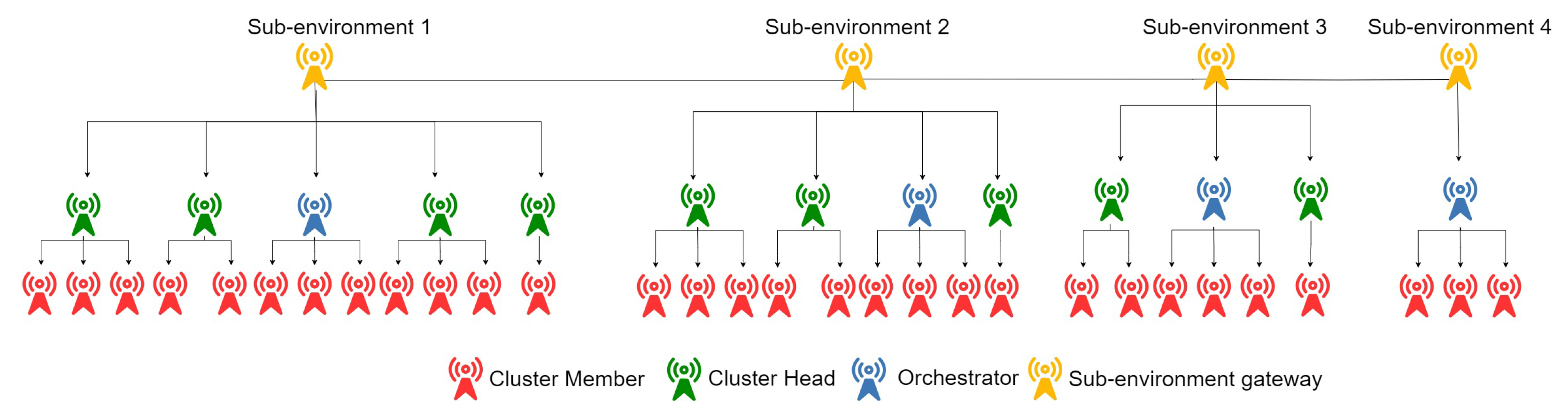
Figure 2 illustrates a global environment divided into four sub-environments after clustering.

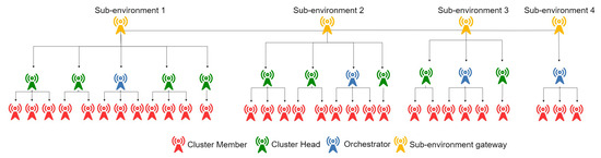
Figure 2. Hierarchical architecture.

We recall that each sub-environment is divided into zones following the devices’ coverage range, and each covered zone has a head (cluster head) responsible for (1) exchanging messages between its child nodes (cluster members) and external nodes using its local index, and (2) distributing the local index of its zone nodes (each having, in the worst case, only two entries which is the current address and the address of the cluster head, $l{i}_{d_j}=\left[\begin{array}{ccc}& z_j& z_x\\ & *& d_{CH}\end{array}\right]$). Thus, when a child node receives a query designated for its zone, it can directly return a response, when possible. On the other hand, when a child node receives a query targeting another zone, it can only forward it to the cluster head (CH), which in its turn will forward it to another CH (when possible), until it reaches the destination. Other local index duplication strategies can also be adopted in many cases (when the child nodes have sufficient capacity, to provide better sustainability, etc.) within a zone by the cluster head (but will not be discussed here). The purpose of using such processing is to reduce the effect of dynamic environments on the index. In other words, updating indexing cluster heads (rather than all devices) will result in a more resilient system, as fewer operations will be necessary.

To establish communication with devices beyond the limits of a sub-environment, the cluster heads route their messages to designated high-capability communication nodes referred to as gateways and elected by the clustering algorithm. In the cluster head’s index, an entry for the cluster gateway is always added (omitted in our illustrative example for the sake of easy representation). The cluster heads can know if a query is for the current sub-environment when targeting a zone inside their limits. Otherwise, they will end up by forwarding the query to the sub-environment gateway. The latter will then forward it to the appropriate sub-environment gateway which, in turn, will route it to the appropriate device or cluster head. It’s worth noting that a sub-environment gateway can also be a cluster head or a simple node.

In the rest of the paper, we will only focus on indexes and queries within a single sub-environment.

5.3. Contribution Insights

In order to detail our proposal, we first present the adopted topology of the connected environment network. Figure 3 shows a sub-environment (extracted from our motivating scenario) that is supervised by one orchestrator $d_o$, having visibility over the related set of sensing nodes deployed. Selected according to its high-capacity (the selection process of super nodes, such as orchestrators, gateways, and cluster heads, is performed in the clustering step and will be detailed in a dedicated study), the orchestrator receives as input the clustered sub-environment details. Then, it generates the sub-environment global index $gi$. The latter can respond to requests but cannot be seen as a routing table. In other words, $gi$ shows the communication between the devices, but it does not show the physical routing of the message. This implies, before assigning a device to a corresponding zone, that we make sure (through the clustering process) that there is a physical link with the related cluster head. After generating $gi$, the orchestrator will be ready to send to each cluster head its corresponding local index $li$. In our motivating scenario, $d4$ was chosen as the sub-environment gateway (during the environment clustering process). Since this device does not interfere in the global index generation, we did not include it inside the global index generation algorithm.

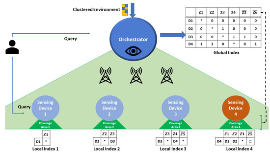
Figure 3. Global & Local Device indexes in a sub-environment.

Sensing devices have specific coverage zones (cf. Definition 4). In essence, given a sensor deployment strategy and an overall number of sensors, $len\left(D\right)$, the sub-environment will contain zones that are covered by one or more sensors, as well as uncovered zones.

The example depicted in Figure 3 shows the sub-environment with the six zones of our motivating scenario (4 are covered: $z_1,z_2,z_3,z_4$ and 2 uncovered: $\overline{z_5},\overline{z_6}$). We recall that a sensing device (1) has one location and can communicate with its cluster head, (2) has a local index, and (3) has a limited storage capacity (e.g., a sensing device can store 4 index entries when its capacity is equal to 4, and (4) cannot store the entire global index. As a result, the orchestrator generates the index entries to be sent to cluster heads for local indexing or in-zone distribution.

Users can then query the environment by submitting queries (q) directly to sensing devices having a specific location stamp l or a zone z. The devices check their local indexes, to decide if they can answer or need to forward to another device. When the desired device is found, it will return its observation o with its corresponding timestamp t. Similarly, queries can be submitted to the orchestrator, which then checks its global index to forward the query to the corresponding devices. The latter case will not be discussed further in this paper.

The main contribution of our proposal relies on determining the right distribution of index entries that need to be stored locally on devices. In other terms, which local index entries are to be stored on each device in order to adequately respond to queries in a timely fashion and maximize the query answering potential over the connected environment zones, while adapting to the different sensing device storage capacities.

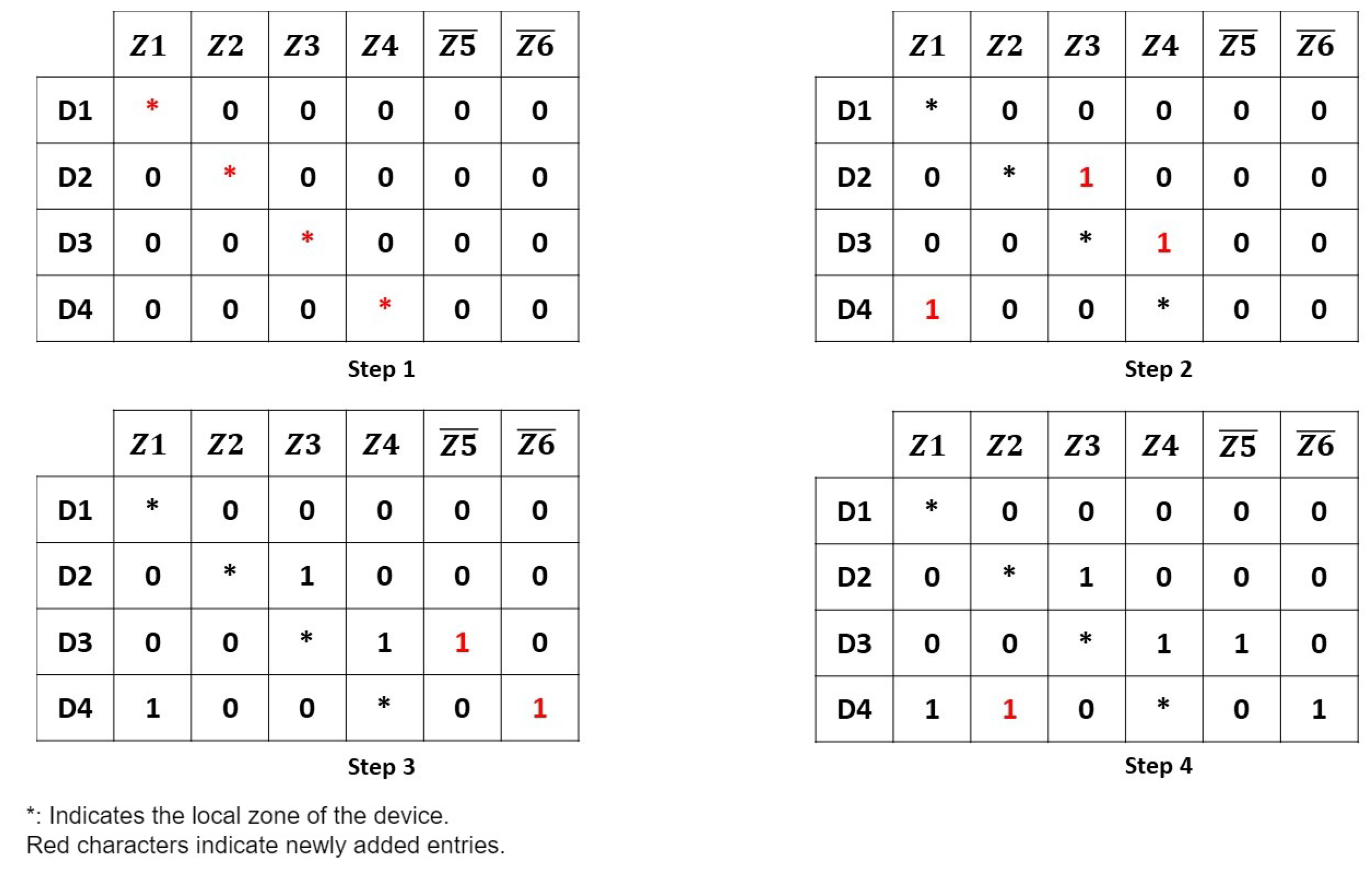
In the following, we focus on the algorithm that generates and distributes the resources’ indexes. It is important to note that in what follows, we will not address how the environment has been clustered, challenges related to sensor deployment, nor device-to-device communication. They will be addressed in separate works. In what follows, we will use the example in Figure 4 to show the main steps of our algorithms. The illustrative example uses four devices, four covered zones, and two uncovered zones.

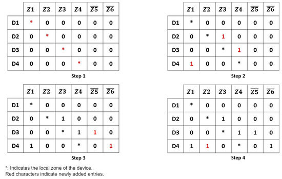
Figure 4. Algorithm steps example with 4 devices, 4 covered (Z1–Z4) and 2 uncovered zones ($\overline{Z5}$–$\overline{Z6}$).

5.4. Index Generation Algorithm

As mentioned before, the global index generation algorithm will be only summarized here. More details can be seen in [2]. We will, however, use a different illustrative use case (a set of devices having different capacities). We note that a global index generation algorithm could be used in many cases (such as for all devices) but we use it in our case for the cluster heads only (following our architecture).

To generate the global index, we use two main algorithms: (1) preprocessing of the global index using Algorithm 1, and (2) add indexes using Algorithm 2 to create a device to zone relation.

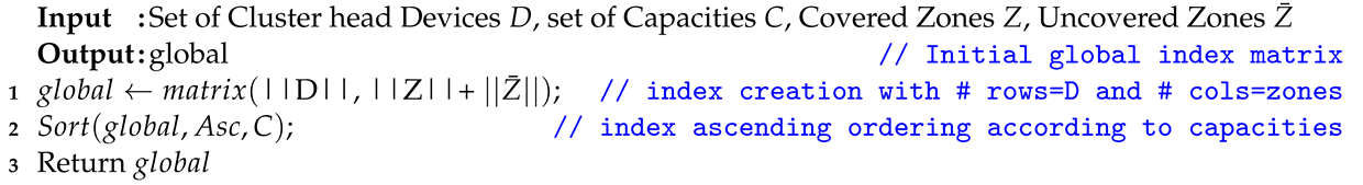
Algorithm 1: PreProcessingGlobalMatrix()

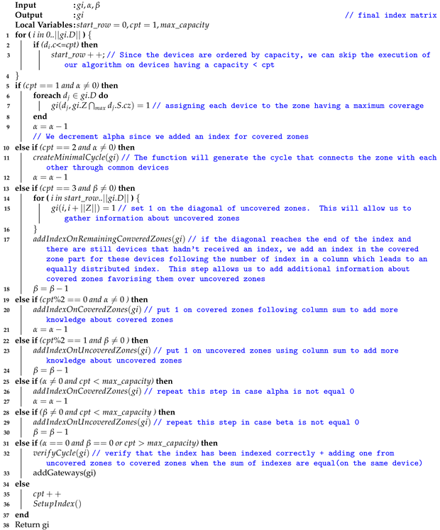
Algorithm 2: SetupIndex()

In Algorithm 1, the preprocessing of the global index matrix on the orchestrator is determined by the components of the sub-environment. Specifically, the number of rows in the matrix corresponds to the number of cluster heads, while the number of columns reflects the total number of zones, encompassing both covered(left side of the index) and uncovered (right side of the index) (line 1).

If the cluster head device’s capacity is the minimum (i.e., 2 in our study), then it has a local index with an entry containing its zone and another entry with the address of a super node (e.g., gateway). If the capacity $d.c$ is sufficient to index all zones (d.c ≥ $\left|\right|Z\left|\right|+\left|\right|\overline{Z}\left|\right|$), the device will contain information about all zones. If the capacity is between the minimum defined and $\left|\right|Z\left|\right|+\left|\right|\overline{Z}\left|\right|$, then Algorithm 2 is applied to generate the final global index.

Algorithm 2 takes the initialized global index from Algorithm 1, $\alpha$ which is the number of entries in the covered zone part of the matrix (defined by the user ) and $\beta$ which is the number of entries in the uncovered zone part of the matrix (defined by the user). In our approach, $\alpha$ must always be greater than $\beta$ to favor covered zones over uncovered zones. In our running example, $\alpha$ equals 3, and $\beta$ equals 1, the four devices ($d1, d2, d3$, and $d4$) have capacities equal to 1, 2, 3, and 4, respectively (after omitting the entry of the related super nodes for each one of them).

We start by obtaining the starting row in the index, to reduce the execution time of the algorithm, since devices that have already maximized their capacity do not need any further processing (lines 1–4).

In lines 5–9, we assign each cluster head device to its zone by detecting its maximum coverage within the environment. This step can be seen in Figure 4 (Step 1). $\alpha$ is decremented by one at the end of this step.

In lines 10–12, we create a minimal cycle between devices for covered zones. The importance of this step is to initiate communication between all the covered zones. The next device entry, when capacity allows, is chosen following a specific distribution strategy to assign the next covered cell (random, biggest capacity, closed, etc.). In our case, we will add an index for the device $D_{i+1}$. Each device will index the zone next to it in the matrix, except the devices whose zones are in the last column. In this case, they add an index for the first zone, since we need to loop between all the covered zones. Step 2 in Figure 4 shows the minimal cycle generation. $d2$ adds an index for $z3$ since $d2$ is located in $z2$ and the location $z3$ is next to the zone $z2$ in the index. For $d4$ an index is added for $z1$, since $\overline{z5}$ is an uncovered zone. $d1$ does not add an index, since it has a capacity of 1.

After creating a minimal cycle and if $\beta$≠ 0, we make a diagonal in the uncovered zones (lines 13–18). With the remaining rows, we index covered zones where the sum of indexes is the lowest. The purpose of doing this is to favor more covered zones over uncovered ones. Figure 4 illustrates in step 3 the result of this step. In our case, $d3$ and $d4$ will add z5 and z6, respectively. At this stage, we can access all the uncovered zones.

Once this is done, we can start alternating between covered and uncovered zones. We add entries for zones having the lowest number of indexes per column. The last matrix of our example demonstrates this step. An index is added for the covered zone $z4$ only, since all the other devices are saturated. $\alpha$ is decremented at the end of this step. We also note that the same functions used above are repeated (lines 19–30) because $\beta$ may become 0 before $\alpha$.

After the algorithm converges (line 31), we check that the indexes are distributed equally between zones and all devices have a number of entries for covered zones greater than uncovered zones’. If this is not the case, we remove entries from uncovered zones and add them to covered zones.In essence, because of variations in the capacities of different devices, certain columns may have more indexes than others. This results in the adjustment of indexes in specific rows, to achieve a more balanced distribution. These verifications are performed using the verify cycle function. In addition, a function called $addGateways\left(\right)$ adds the corresponding gateway for each device. After generating the matrix, the global index is ready to be cut by rows and distributed over the devices. In order to simplify the global index final representation, we did not include the cluster gateway inside the resulting global index (Figure 4 step 4). We note that, in cases where the number of devices is higher than the number of zones, the index will have more rows than columns, while having more zones than devices will lead to a number of columns greater than the number of rows(such as in our example). If the number of devices is equal to the number of zones, the rows and the columns will be equal.

5.5. Local Index Generation

Once the previous algorithms have been applied, the global index is ready to be distributed over the cluster heads. It is divided by device as a vector of zones. Only completed entries in the initial $gi$ (containing 1 value) are considered in the local index (i.e., all 0 values corresponding to columns are removed). In addition, the cell values are transformed as follows: (1) values ‘*’ indicate local zones covered by the corresponding device, (2) zones marked with device identifiers indicate to whom queries must be forwarded, while (3) zones marked with “□” indicate uncovered zones.

Query execution simulations were implemented. As cited before, the difference in user needs implies implementing many query types. We will demonstrate the methodology of the execution of each type. In the following figures, straight arrows indicate the index chosen by the device, while dotted arrows show the device to which the message is forwarded. After arriving at the destination zone, the device will return the message using the path found (the path followed must be saved inside the message). The following query processing is performed on the local index of the cluster head and not on the global index (orchestrator). Many algorithms could be employed to return the response optimally (further studies could be made on these algorithms). When the message passes through all the devices inside a zone, we prevent the message from re-entering the zone, to avoid loops inside the index.

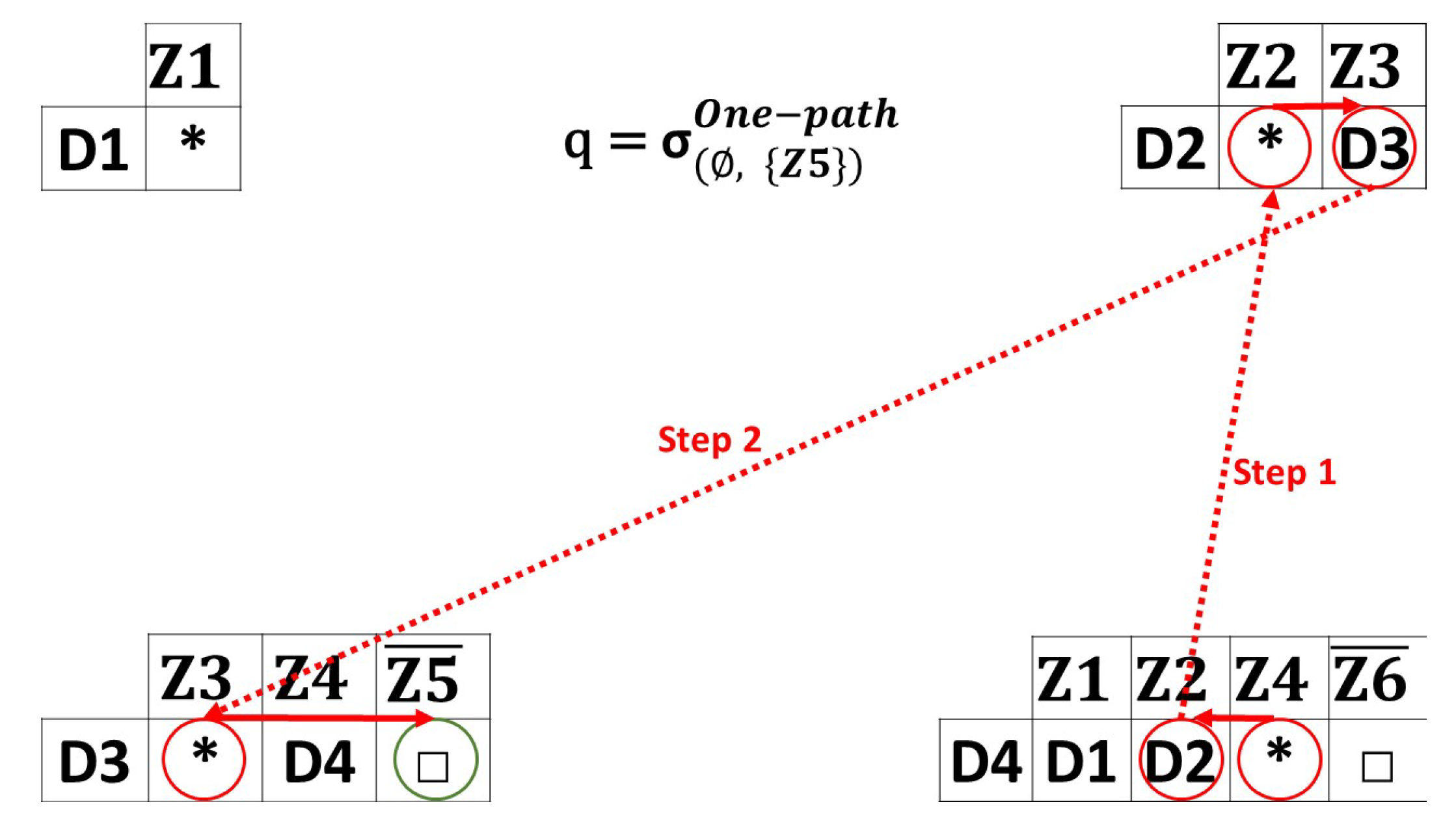
• One-path Queries: Figure 5 illustrates an example of one-path queries taking a random path strategy. We consider that a query from the location $z4$ to $\overline{z5}$ is sent. The device $d4$ located in $z4$ receives the query. $d4$ does not know any information about $\overline{z5}$. In that case, the query is forwarded to a randomly chosen covered zone. In this situation, $z2$ is chosen. The device located in $z2$ is device $d2$, meaning that this device receives the query (step 1). The query is forwarded to $z3$, since $d2$ is partially covered by $d3$ only. The query is forwarded to device $d3$ (step 2). $d3$ has an index for $\overline{z5}$ leading to forwarding the query to the user, with a response that $\overline{z5}$ is an uncovered zone. When a blocked path is faced, a “no response” message is returned for the user by the last device reached. This type of query can be used to gather data in order to perform analytics where having missing data is not important.
  

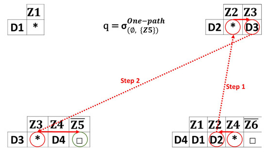  Figure 5. One-path queries example.
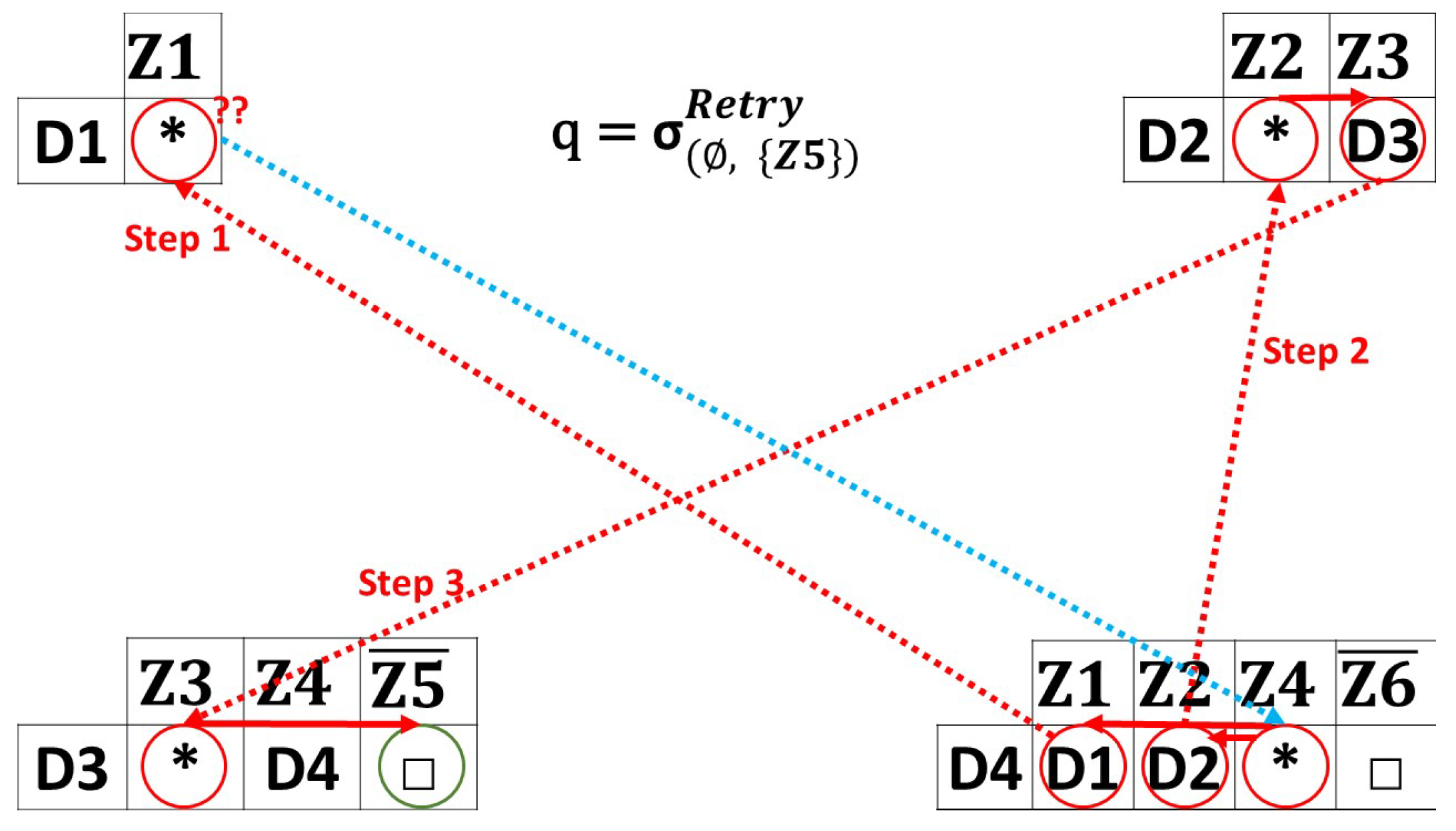
• Retry Queries: Figure 6 shows the cases of retrying queries with a random strategy. In this case, the source zone is $z4$, and the destination zone is $\overline{z5}$. In Figure 6, the query is first sent to $d4$, which chooses a random device from its index to forward the query. $d4$ chooses, for instance, to forward it to $d1$. Since $d1$ has a capacity of 1, it has no information about any zone except its current zone. As a result, it is no longer possible for $d1$ to continue forwarding the query, indicating that the path is blocked (even though the device has an index for its gateway, the query is not forwarded to the gateway, since the query is designated for the current sub-environment). Consequently, the query is returned to $d4$, trying to find another path. The query is re-sent to $d2$. After $d2$ receives the query, it forwards it to $d3$. $d3$ returns an uncovered zone response to the user. When a blocked path is faced and no more devices are in the current coverage zone, a “no-response” message is returned to the user. The following queries are used for model training, reducing missing data and making the preprocessing easier.
  

  Figure 6. Retry queries example.
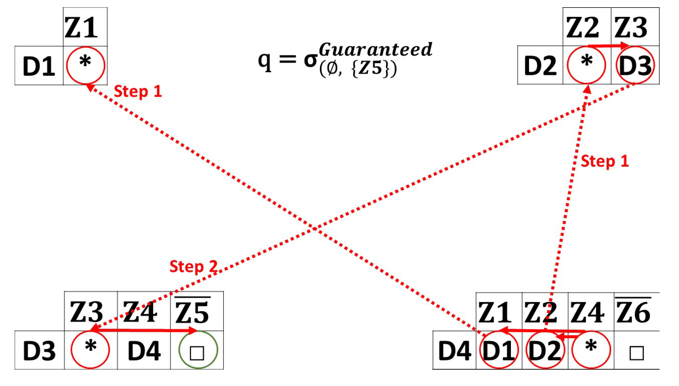
• Guaranteed queries: Figure 7 presents an example of a guaranteed query. $z4$ is the source zone and $\overline{z5}$ is the destination zone. $d4$ sends a broadcast request to $d1$ and $d2$. $d1$ is a blocked path, so the query ends here for the first path. For the second path, the query continues until reaching $d3$, having information about $\overline{z5}$. If there is no path that leads to the requested destination, a no-response message is returned. These queries are for high-urgency cases such as fires and natural disasters.
  

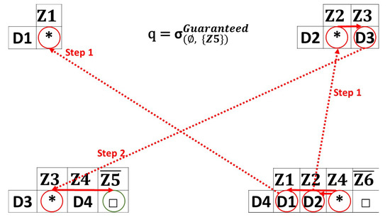  Figure 7. Guaranteed queries example.
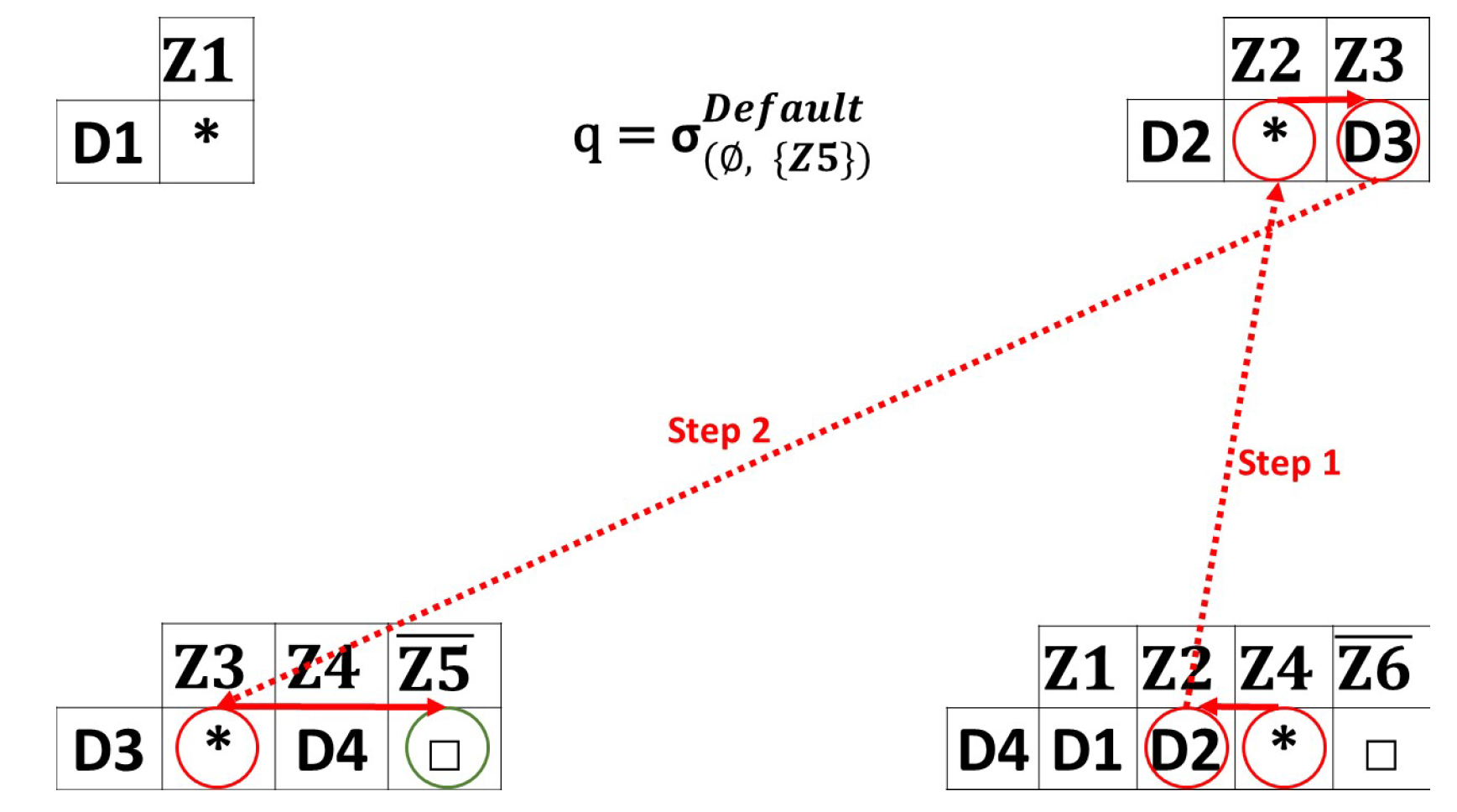
• Default queries: Figure 8 demonstrates an example of a default query. Recall that guaranteed and default queries work in almost the same way, since the default queries have extra parameters (in our case, we consider a minimum capacity equal or greater to 2). The same source/destination zones are used ($z4$ to $\overline{z5}$). Once $d4$ receives the query, it broadcasts it to all its index entries that fit the criteria selected. The same process is repeated until the desired destination zone is reached. Notice that the query is not routed to $d1$, due to its limited capacity, which is insufficient for accommodating a value greater than two. In this example, $d3$ returns the result (uncovered zone) for the user. A no-response message is returned if no path leads to the requested destination. These queries are designed for high-urgency cases, such as fires and natural disasters, with an emphasis on minimizing the utilization of network resources.
  

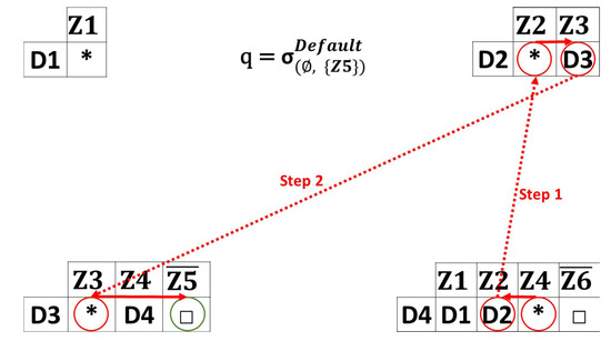  Figure 8. Default queries example.

6. Experiments

In the upcoming section, we describe a series of experiments carried out to confirm the efficacy of our approach. Through this evaluation, we measured the performance of our approach regarding: (1) the index generation, (2) the index coverage, and (3) the execution of different types of queries. The experiments were executed on a computer system equipped with 16 GB of RAM, a Core i7 CPU, and running the Windows 10 operating system. In addition, in all tests, we used a coverage percentage of 80% and an overlap (covered zones with more than one device) of 70%, to ensure that we had a diversity in zone types (covered zones with multiple devices, covered zones with one device, and uncovered zones).

In this evaluation, we abstained from performing a comparative analysis with other approaches because, as indicated in Section 3, none of them can meet all the required criteria with their indexing scheme. The environment data and all the tests were simulated using our generator (https://sigappfr.acm.org/Projects/RILCE/, accessed on 29 November 2023). The execution time was averaged over ten runs for each result data point. We also note that we did not include cluster gateways inside global indexes, since this was chosen by the clustering algorithm. In addition, we generated large environments that were complex to index.

6.1. Index Generation

The first set of experiments was dedicated to evaluating index creation by measuring the time needed to create our index containing covered and uncovered zones. To observe its behavior, we varied several parameters: the number of zones, number of devices, values of the two parameters $\alpha$ and $\beta$, and devices’ capacities. The results of these test can be see in [2].

6.2. Index Coverage

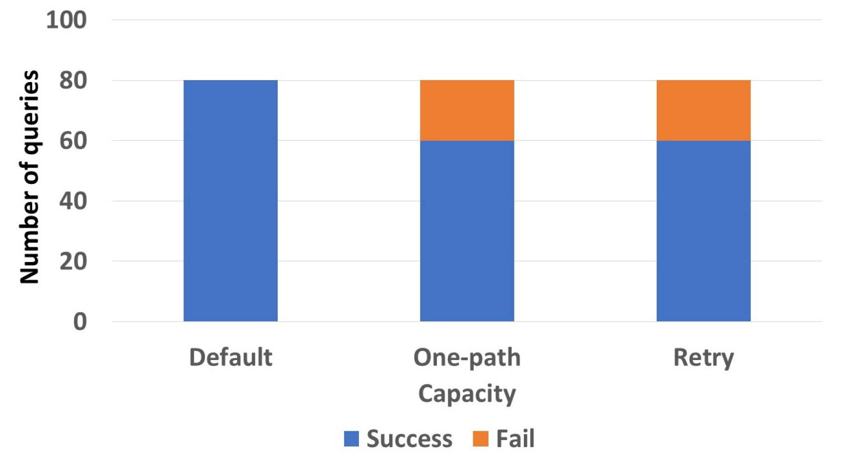
In the following section, testing was conducted on an environment composed of 3000 devices distributed over 300 zones. The goal of this experiment was to demonstrate the impact of the device’s capacity on the query response. In Figure 9, we considered that all the devices had the same capacity, equal to 8. We can see that 80/80 default queries gave a response, while one-path and retry queries gave 60/80 successful responses. This shows that our indexing scheme is more than satisfactory in terms of priority, since it provides a proper coverage for different types of queries having different urgency levels using limited storage capacities. Note that we assumed a capacity of 8 since this was the first value where all default queries returned a response.

Figure 9. Capacity to response effect.

6.3. Query Execution

In the next sets of experiments, we aimed to test the effectiveness of our algorithm by evaluating the results of different types of queries, along with their execution time. Using an environment with 300 zones and 3000 devices, the query responses included queries issued for both covered and uncovered destination. It is important to note that queries were generated using our generator. When comparing query types, the same source zones and destination zones were used. However, when comparing different environments (different zones and devices) different queries were used, since the environments were not the same. During the query execution experiments, we employed a random strategy (random path) for one-path and retry queries. We note that we could not compare the query execution approach to other approaches because we can follow their strategy through the function.

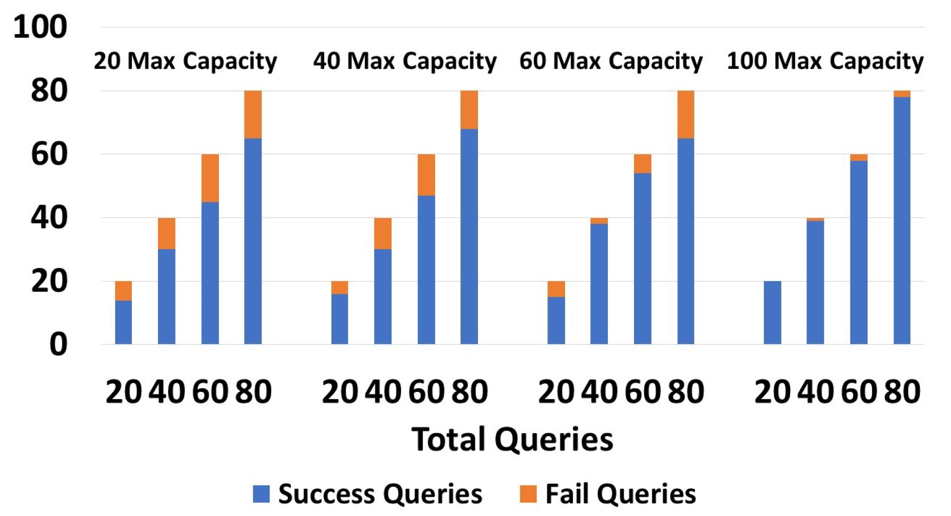
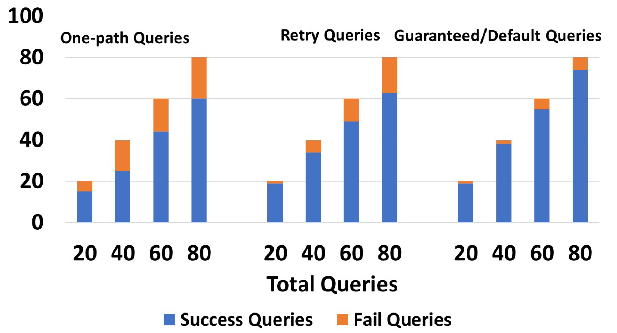
Figure 10 shows the execution of one-path queries (We recall that the query types were explained in detail in Section 4.3), with devices having capacities of 20, 40, 60, and 100. As shown in the graph, devices having a capacity of 20 returned 11/20 and 54/80 successful queries, while devices having a capacity of 100 returned 18/20 and 77/80 successful queries. As the capacity increased, the number of successful queries increased. We tried with 20, 40, 60, and 80 queries, and in all cases, the number of successful queries grew with the capacity increase. In the right-side graphic in Figure 10, with devices having a capacity of 100, the number of queries with no results was low. In Figure 11, retry queries were used with corresponding results on devices having capacities of 20, 40, 60, and 100. We obtained the following results: 14/20 and 65/80 were successful queries for devices having c = 20, while for c = 100, 20/20 and 78/100 were successful queries. We obtained more successful queries than the one-path queries, due to the capability to resend the query to another zone in case of failure. We can see that in the four tests, in all cases (20, 40, 60, and 80), the number of successful queries increased as the capacity grew. We can also see that the number of queries that did not give a response with a capacity of 100 was very low. Moreover, it is worth noting that retry queries yielded a greater number of responses compared to one-path queries, particularly on devices with limited capacities. In Figure 12, guaranteed and default queries always responded regardless of the devices’ capacity (20, 40, 60, 100), since they tried all possible paths.

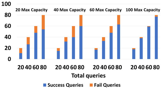
Figure 10. Success/failures in one-path queries.

Figure 11. Success/failures in retry queries.

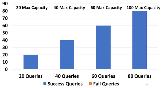
Figure 12. Success/failures in guaranteed queries.

In Figure 13, we evaluated the execution time for all query types. This was performed using an environment with 300 zones and 3000 devices. Obviously, one-path queries took the least time to execute (0.145 s), since they followed one path. In contrast, the default queries took the most time (0.192 s), since they required consequent processing before trying all possible paths. The expected results were reached during these experiments.

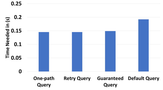
Figure 13. Different query type time executions.

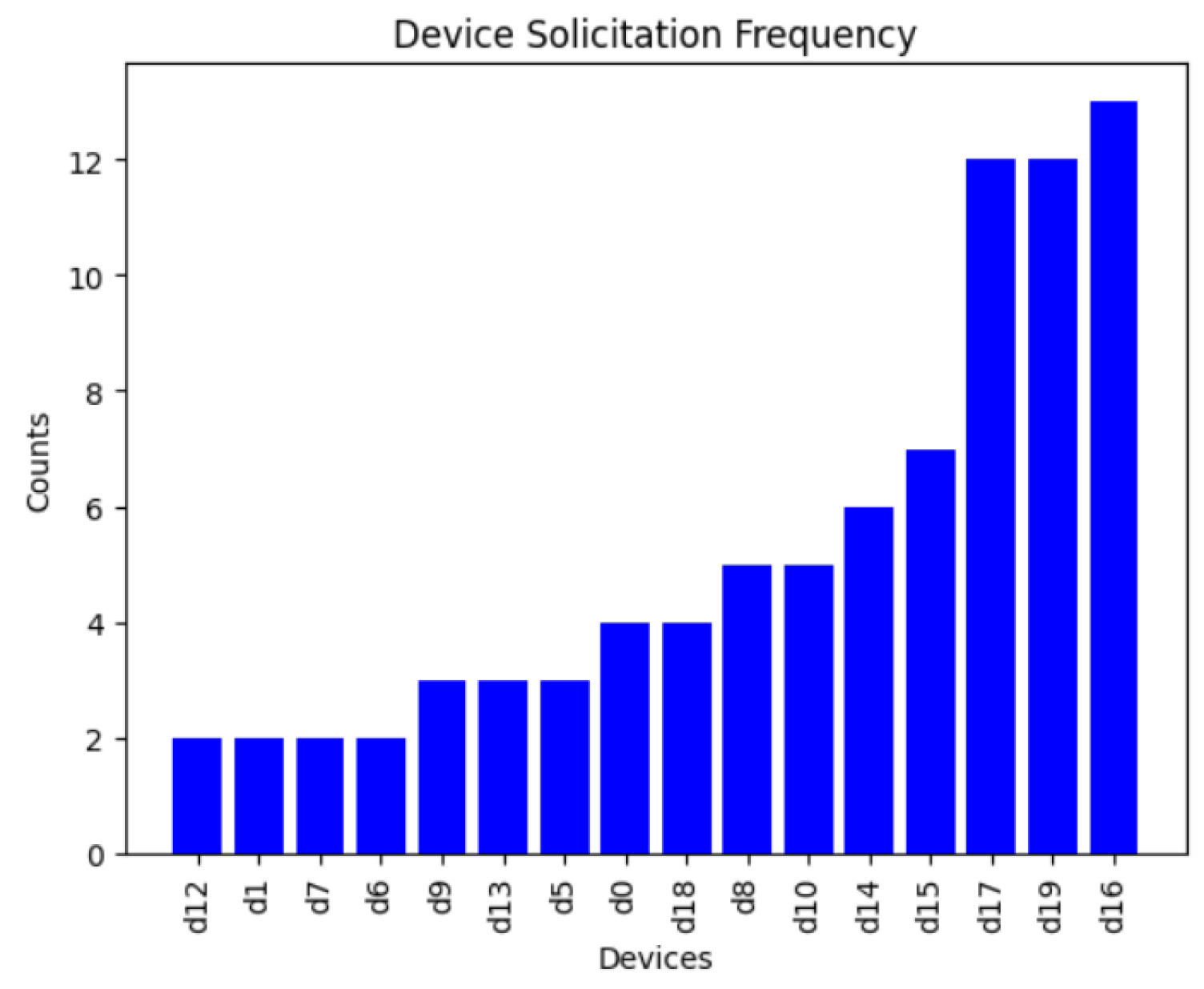
6.4. Device Solicitation Experiment

During this experiment, we generated an environment of 10 zones and 20 devices, in which 10 of the devices had a capacity equal to 1 or 2. Twenty queries were executed during the experiment. As we can see in Figure 14 and Figure 15, the total number of devices solicited for one-path queries was 85, while for retry queries, the number of devices solicited was 75, depending on the path taken. For guaranteed queries, since this is a broadcast query, all the devices were solicited, meaning that the total number of devices solicited is 20 × 20 = 400. However, for the default type of query, if we set the condition that the device had to have a capacity greater than 2 in order to be involved, the number of devices solicited was 10 × 20 = 200. Since one-path queries took the least amount of time to execute and only specific number of devices were involved they consumed the least amount of resources. Conversely, the default queries took the longest time and more devices were involved in this type of query, indicating that they consumed more resources than the other queries.

Figure 14. Device solicitation for one-path queries.

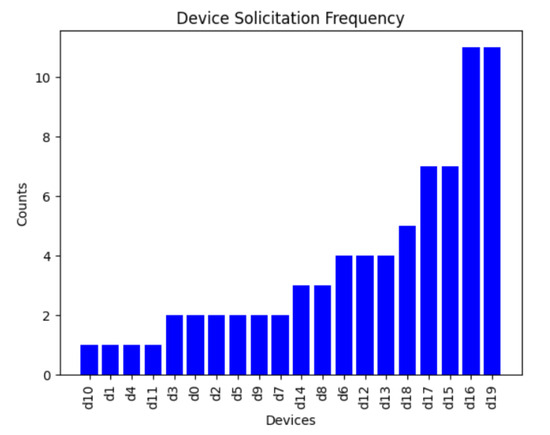
Figure 15. Device solicitation for retry queries.

6.5. Array of Things Experiments

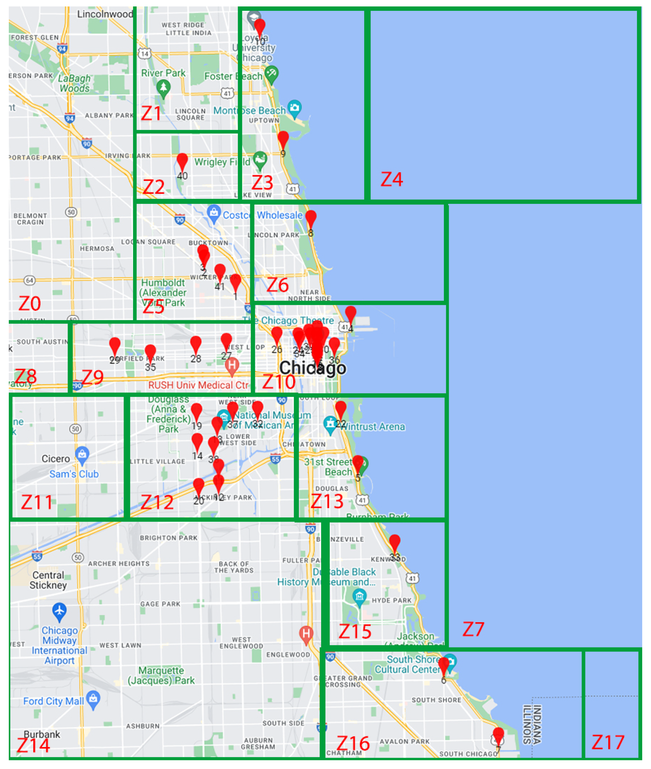
To add further experiments on a real-scenario, we used the dataset from the project named “array of things” organized by the urban center for computation and data and others in Chicago. (https://arrayofthings.github.io/index.html, accessed on 29 November 2023) This dataset contains data concerning the location of different devices distributed in the city of Chicago, such as the location name and type (lakeshore, for example), the status (live, pending), the longitude, and the latitude. We placed the different device locations on a map, to visualize and cluster them into different zones. We note that a capacity of the devices was considered between 1 and 18 ($1<C_d<18$).

As shown in Figure 16, the clustered environment contained 18 zones (10 covered and 8 uncovered) and 41 devices. The index was generated with $\alpha =10$ and $\beta =8$. It took 0.0087 s to generate the index (Table 2). We also note that all devices were included inside the index in this example.

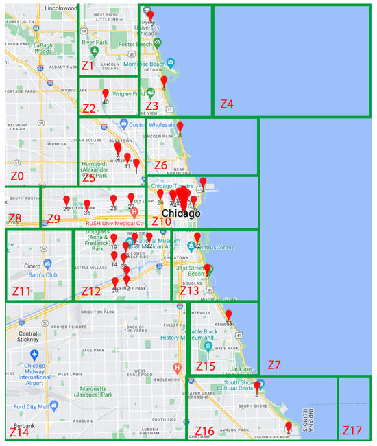
Figure 16. The clustered map of the “Array of things” project.

Table 2. The generated index of the “Array of things” project.

	z2	z12	z9	z10	z6	z3	z5	z16	z15	z13	z0	z1	z4	z7	z8	z11	z14	z17
d40	*	0	0	0	0	0	0	0	0	0	0	0	0	0	0	0	0	0
d11	0	*	0	0	0	0	0	0	0	0	0	0	0	0	0	0	0	0
d28	0	0	*	0	0	0	0	0	0	0	0	0	0	0	0	0	0	0
d34	0	0	0	*	0	0	0	0	0	0	0	0	0	0	0	0	0	0
d13	0	*	1	0	0	0	0	0	0	0	0	0	0	0	0	0	0	0
d8	0	0	0	0	*	1	0	0	0	0	0	0	0	0	0	0	0	0
d29	0	0	*	1	0	0	0	0	0	0	1	0	0	0	0	0	0	0
d32	0	*	1	0	0	0	0	0	0	0	0	1	0	0	0	0	0	0
d12	0	*	1	0	0	0	0	0	0	1	1	0	0	0	0	0	0	0
d30	0	0	0	*	1	0	1	0	0	0	0	1	0	0	0	0	0	0
d35	0	0	*	1	0	0	0	1	0	0	0	0	1	0	1	0	0	0
d10	0	0	0	0	0	*	1	0	1	0	0	0	0	1	0	1	0	0
d15	0	0	0	*	1	0	0	0	0	1	0	0	0	0	1	0	1	0
d26	1	0	0	*	1	0	0	0	0	0	0	0	0	0	0	1	0	1
d20	1	*	1	0	0	1	0	0	0	0	0	0	0	0	0	0	1	0
d24	0	1	0	*	1	1	0	0	0	0	0	1	0	0	0	0	0	1
d14	0	*	1	0	0	0	1	0	1	0	1	0	1	0	0	0	0	0
d27	0	0	*	1	0	0	0	1	0	1	0	1	0	1	0	0	0	0
d23	1	0	0	*	1	0	0	0	1	0	0	0	1	0	1	0	0	0
d36	0	0	0	*	1	1	0	0	0	1	0	0	0	1	0	1	0	0
d2	1	0	0	0	0	0	*	1	1	0	0	0	0	0	1	0	1	0
d6	1	1	0	0	0	0	0	*	1	1	0	0	0	0	0	1	0	1
d9	1	1	0	0	0	*	1	1	0	0	1	0	0	0	0	0	1	0
d38	0	*	1	0	0	1	1	1	0	0	0	1	0	0	0	0	0	1
d21	0	0	1	*	1	1	0	0	1	0	1	0	1	1	0	0	0	0
d33	1	1	0	0	0	1	0	0	*	1	0	1	0	1	1	0	0	0
d25	0	0	0	*	1	1	1	0	1	1	0	0	1	0	1	1	0	0
d37	0	*	1	0	1	1	0	1	0	1	0	0	0	1	0	1	1	0
d3	1	1	0	0	0	0	*	1	1	1	0	0	0	0	1	1	1	1
d18	0	0	0	*	1	1	1	1	1	0	1	0	0	0	1	1	0	1
d4	1	0	0	*	1	0	1	1	1	0	1	1	0	0	0	0	1	1
d5	1	1	0	0	0	1	1	1	0	*	0	1	1	0	0	0	1	1
d16	1	1	1	*	1	0	0	0	1	1	1	1	1	1	0	0	0	0
d1	1	0	1	0	0	1	*	1	1	1	1	1	1	1	1	0	0	0
d19	1	*	1	0	1	0	1	1	0	1	1	0	1	1	1	1	0	0
d17	0	1	1	*	1	1	1	1	1	0	0	0	1	1	1	1	1	0
d31	1	0	1	*	1	1	1	0	1	1	0	1	0	1	1	1	1	1
d22	1	1	0	1	1	1	1	1	1	*	1	0	1	0	1	1	1	1
d39	1	1	1	1	1	1	1	1	1	1	1	1	1	1	0	1	1	1
d41	1	1	1	1	1	1	1	1	1	1	1	1	1	1	1	1	1	1
d7	1	1	1	1	1	1	1	1	1	1	1	1	1	1	1	1	1	1

Red columns are uncovered zones.

After generating the global index, we executed 20, 40, 60, and 80 queries. We determined the results shown in Figure 17. One-path queries gave 18/20, 37/40, 55/60, and 70/80 responses, while retry queries gave 19/20, 39/40, 59/60, and 76/80 responses. Some guaranteed and default queries did not give a response because, in zone $z2$, there was one device $d40$ with a capacity of 1. Given its capacity of one, it possessed no information beyond its present zone. Any query issued from that device requesting information from another zone did not give a response, since the following device only had information about its local zone. These results were expected, since one-path and retry queries choose one path, while guaranteed and default queries will try all possible paths.

Figure 17. Success/Failures of the queries for the array of things project.

Figure 18 shows the execution time of each query type on this dataset. We used the same source and destination zone in the four cases. The query issued went from $z8$ to $z12$. One-path queries took 0.0059 s, retry queries took 0.0062 s, guaranteed queries took 0.0138, and default queries took 0.0146. Guaranteed and default queries took the longest execution time, because they explored all potential routes. The increased execution time of the default queries can be attributed to their pre-processing tasks, which involved, for example, directing traffic toward highly indexed devices.

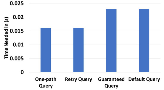
Figure 18. Query time execution for the array of things project.

6.6. Discussion

Following these results, we can see that our approach produced good results, especially in environments having high-capacity devices. During the index generation, we noticed that our approach was linear regarding zones, while being quadratic in terms of the device. In other words, incorporating devices into our approach required more time compared to the time needed for adding zones. Some queries (like one-path and retry) did not produce responses for environments with low-capacity devices, depending on the number and density of zones. Other types of queries showed a high potential, even when low-capacity devices were encountered, such as guaranteed and default queries. These types of queries can consume more resources (energy) and time, since many devices may be involved and processing is required at some point. All these use cases depend on the user’s needs.

7. Conclusions

In this paper, we proposed a new solution for indexing and querying resources in connected environments. Numerous types of research have been conducted regarding this subject, but the majority did not consider device capacity, covered/uncovered zones, and query types. Additionally, a hybrid overlay architecture was introduced, enhancing the robustness of the index for dynamic environments. The global index generation algorithm consisted of different steps to index the device and had the ability to discover information about covered and uncovered zones, increasing the network life cycle. Moreover, the algorithm took into consideration devices having different capacities (a device cannot store all environment information). Each device was indexed according to its capability. Moreover, various query and response types were introduced to align with user requirements. One-path queries follow one path with a specific strategy, retry queries follow one path with correction capability, and guaranteed and default queries search among all available paths. Different evaluations were performed and produced different results. The challenge of clustering an environment into different zones will be analyzed in future works. Furthermore, more tests will be conducted in real scenarios to evaluate the performance of our approach in various contexts.

References

- Hasan, M. State of IoT 2022: Number of Connected IoT Devices Growing 18% to 14.4 Billion Globally. 2022. Available online: https://iot-analytics.com/number-connected-iot-devices/ (accessed on 29 November 2023).
- Achkouty, F.; Mansour, E.; Gallon, L.; Corral, A.; Chbeir, R. RILCE: Resource Indexing in Large Connected Environments. In New Trends in Database and Information Systems, ADBIS 2023, Proceedings of the European Conference on Advances in Databases and Information Systems, Barcelona, Spain, 4–7 September 2023; Springer: New York, NY, USA, 2023; pp. 13–22. [Google Scholar]
- Fathy, Y.; Barnaghi, P.; Tafazolli, R. Large-Scale Indexing, Discovery, and Ranking for the Internet of Things (IoT). ACM Comput. Surv. 2018, 51, 29:1–29:53. [Google Scholar] [CrossRef]
- Kamel, M.B.; Crispo, B.; Ligeti, P. A decentralized and scalable model for resource discovery in IoT network. In Proceedings of the 2019 International Conference on Wireless and Mobile Computing, Networking and Communications (WiMob), Barcelona, Spain, 21–23 October 2019; IEEE: New York, NY, USA, 2019; pp. 1–4. [Google Scholar]
- Li, Z.; Chen, R.; Liu, L.; Min, G. Dynamic resource discovery based on preference and movement pattern similarity for large-scale social internet of things. IEEE Internet Things J. 2015, 3, 581–589. [Google Scholar] [CrossRef]
- Paganelli, F.; Parlanti, D. A DHT-Based Discovery Service for the Internet of Things. J. Comput. Netw. Commun. 2012, 2012, 107041. [Google Scholar] [CrossRef]
- Cassar, G.; Barnaghi, P.M.; Moessner, K. Probabilistic Methods for Service Clustering. In Proceedings of the SMRR@ISWC Workshop, Shanghai, China, 8 November 2010. [Google Scholar]
- Wang, W.; De, S.; Cassar, G.; Moessner, K. An experimental study on geospatial indexing for sensor service discovery. Expert Syst. Appl. 2015, 42, 3528–3538. [Google Scholar] [CrossRef]
- Elmahi, M.Y.; Osman, N.; Hamza, H.S. Resource discovery classification for internet of things: A survey. Int. J. Digit. Inf. Wirel. Commun. 2020, 10, 35–50. [Google Scholar] [CrossRef]
- Ponnusamy, K.; Rajagopalan, N. Internet of things: A survey on IoT protocol standards. In Progress in Advanced Computing and Intelligent Engineering: Proceedings of ICACIE 2016, Volume 2; Springer Publishing Company, Incorporated: New York, NY, USA, 2018; pp. 651–663. [Google Scholar]
- Bormann, C.; Castellani, A.P.; Shelby, Z. Coap: An application protocol for billions of tiny internet nodes. IEEE Internet Comput. 2012, 16, 62–67. [Google Scholar] [CrossRef]
- Goland, Y.Y. Simple Service Discovery Protocol/1.0 Operating without on Arbiter. IETF INTERNET-DRAFT draft-cai-ssdp-v1-03. txt. 1999. Available online: https://link.springer.com/chapter/10.1007/978-3-540-30184-4_20 (accessed on 29 November 2023).
- Butt, T.A.; Phillips, I.; Guan, L.; Oikonomou, G. TRENDY: An adaptive and context-aware service discovery protocol for 6LoWPANs. In Proceedings of the Third International Workshop on the Web of Things, Newcastle, UK, 19 June 2012; pp. 1–6. [Google Scholar]
- Lee, K.; Kim, S.; Jeong, J.P.; Lee, S.; Kim, H.; Park, J.S. A framework for DNS naming services for Internet-of-Things devices. Future Gener. Comput. Syst. 2019, 92, 617–627. [Google Scholar] [CrossRef]
- Razzaque, M.A.; Milojevic-Jevric, M.; Palade, A.; Clarke, S. Middleware for internet of things: A survey. IEEE Internet Things J. 2015, 3, 70–95. [Google Scholar] [CrossRef]
- Cirani, S.; Davoli, L.; Ferrari, G.; Léone, R.; Medagliani, P.; Picone, M.; Veltri, L. A scalable and self-configuring architecture for service discovery in the internet of things. IEEE Internet Things J. 2014, 1, 508–521. [Google Scholar] [CrossRef]
- Djamaa, B.; Yachir, A.; Richardson, M. Hybrid CoAP-based resource discovery for the Internet of Things. J. Ambient. Intell. Humaniz. Comput. 2017, 8, 357–372. [Google Scholar] [CrossRef]
- Alam, S.; Noll, J. A semantic enhanced service proxy framework for internet of things. In Proceedings of the 2010 IEEE/ACM Int’l Conference on Green Computing and Communications & Int’l Conference on Cyber, Physical and Social Computing, Hangzhou, China, 18–20 December 2010; IEEE: New York, NY, USA, 2010; pp. 488–495. [Google Scholar]
- Chirila, S.; Lemnaru, C.; Dinsoreanu, M. Semantic-based IoT device discovery and recommendation mechanism. In Proceedings of the 2016 IEEE 12th International Conference on Intelligent Computer Communication and Processing (ICCP), Cluj-Napoca, Romania, 8–10 September 2016; IEEE: New York, NY, USA, 2016; pp. 111–116. [Google Scholar]
- Bröring, A.; Datta, S.K.; Bonnet, C. A categorization of discovery technologies for the internet of things. In Proceedings of the 6th International Conference on the Internet of Things, Stuttgart, Germany, 7–9 November 2016; pp. 131–139. [Google Scholar]
- Pozza, R.; Nati, M.; Georgoulas, S.; Gluhak, A.; Moessner, K.; Krco, S. CARD: Context-aware resource discovery for mobile Internet of Things scenarios. In Proceedings of the IEEE International Symposium on a World of Wireless, Mobile and Multimedia Networks 2014, Washington, DC, USA, 19 June 2014; IEEE: New York, NY, USA, 2014; pp. 1–10. [Google Scholar]
- Jiang, Y.; Guo, S.; Xu, S.; Qiu, X.; Meng, L. Resource discovery and share mechanism in disconnected ubiquitous stub network. In Proceedings of the NOMS 2018—2018 IEEE/IFIP Network Operations and Management Symposium, Taipei, Taiwan, 23–27 April 2018; IEEE: New York, NY, USA, 2018; pp. 1–7. [Google Scholar]
- Misra, S.; Barthwal, R.; Obaidat, M.S. Community detection in an integrated Internet of Things and social network architecture. In Proceedings of the 2012 IEEE Global Communications Conference (GLOBECOM), Anaheim, CA, USA, 3–7 December 2012; IEEE: New York, NY, USA, 2012; pp. 1647–1652. [Google Scholar]
- Ratnasamy, S.; Karp, B.; Yin, L.; Yu, F.; Estrin, D.; Govindan, R.; Shenker, S. GHT: A geographic hash table for data-centric storage. In Proceedings of the 1st ACM International Workshop on Wireless Sensor Networks and Applications, Atlanta, GA, USA, 28 September 2002; pp. 78–87. [Google Scholar]
- Greenstein, B.; Ratnasamy, S.; Shenker, S.; Govindan, R.; Estrin, D. DIFS: A distributed index for features in sensor networks. Ad Hoc Netw. 2003, 1, 333–349. [Google Scholar] [CrossRef]
- Fathy, Y.; Barnaghi, P.; Tafazolli, R. Distributed spatial indexing for the Internet of Things data management. In Proceedings of the 2017 IFIP/IEEE Symposium on Integrated Network and Service Management, Lisbon, Portugal, 8–12 May 2017; IEEE: New York, NY, USA, 2017; pp. 1246–1251. [Google Scholar]
- Fathy, Y.; Barnaghi, P.; Enshaeifar, S.; Tafazolli, R. A distributed in-network indexing mechanism for the Internet of Things. In Proceedings of the 2016 IEEE 3rd World Forum on IoT, Reston, VA, USA, 12–14 December 2016; pp. 585–590. [Google Scholar]
- Tang, J.; Xiao, Y.; Zhou, Z.; Shu, L.; Wang, Q. An energy efficient hierarchical clustering index tree for facilitating time-correlated region queries in wireless sensor network. In Proceedings of the 2013 9th Int. Wireless Communications and Mobile Computing Conference, Sardinia, Italy, 1–5 July 2013; IEEE: New York, NY, USA, 2013; pp. 1528–1533. [Google Scholar]
- Zhou, Z.; Zhou, Z.; Niu, J.; Wang, Q. EGF-tree: An energy-efficient index tree for facilitating multi-region query aggregation in the internet of things. Pers. Ubiquitous Comput. 2014, 18, 951–966. [Google Scholar] [CrossRef]
- Hoseinitabatabaei, S.A.; Fathy, Y.; Barnaghi, P.; Wang, C.; Tafazolli, R. A novel indexing method for scalable iot source lookup. IEEE Internet Things J. 2018, 5, 2037–2054. [Google Scholar] [CrossRef]
- Benrazek, A.E.; Kouahla, Z.; Farou, B.; Ferrag, M.A.; Seridi, H.; Kurulay, M. An efficient indexing for Internet of Things massive data based on cloud-fog computing. Trans. Emerg. Telecommun. Technol. 2020, 31, e3868. [Google Scholar] [CrossRef]
- Dong, C.; Jiang, L.; Wang, K. IoT Search Method for Entity Based on Advanced Density Clustering. In Proceedings of the 2020 Information Communication Technologies Conference, Nanjing, China, 29–31 May 2020; IEEE: New York, NY, USA, 2020; pp. 64–69. [Google Scholar]
- Huang, C.Y.; Chang, Y.J. An adaptively multi-attribute index framework for big IoT data. Comput. Geosci. 2021, 155, 104841. [Google Scholar] [CrossRef]
Disclaimer/Publisher’s Note: The statements, opinions and data contained in all publications are solely those of the individual author(s) and contributor(s) and not of MDPI and/or the editor(s). MDPI and/or the editor(s) disclaim responsibility for any injury to people or property resulting from any ideas, methods, instructions or products referred to in the content. |
© 2023 by the authors. Licensee MDPI, Basel, Switzerland. This article is an open access article distributed under the terms and conditions of the Creative Commons Attribution (CC BY) license (https://creativecommons.org/licenses/by/4.0/).