Abstract
Wireless communication tower placement arises in many real-world applications. This paper investigates a new emerging wireless communication tower placement problem, namely, continuous space wireless communication tower placement. Unlike existing wireless communication tower placement problems, which are discrete computational problems, this new wireless communication tower placement problem is a continuous space computational problem. In this paper, we formulate the new wireless communication tower placement problem and propose a hybrid simulated annealing algorithm that can take advantage of the powerful exploration capacity of simulated annealing and the strong exploitation capacity of a local optimization procedure. We also demonstrate through experiments the effectiveness of this hybridization technique and the good performance and scalability of the hybrid simulated annulling in this paper.
1. Introduction
Wireless communication tower placement arises in many real-world applications. For example, in the deployment of a 5G communication network, we need to place a set of base stations in a geographical area such that the 5G users in the area can send and receive data through those base stations [1]; in the deployment of a network-based real-time kinematic (RTK) positioning service, we need to place a set of Continuously Operating Reference Stations (CORSs) to receive GPS measurements from satellites and process the GPS measurements to generate positioning corrections and broadcast the corrections to the users of the network RTK positioning service [2]; and in the deployment of a wireless sensor network, we need to determine where the sensors should be placed in order to minimize communication delay and energy consumption [3]; etc.
Wireless communication tower placement is an important problem in the design and deployment of a wireless communication network. The aim is to find an optimal placement of wireless communication towers, which is usually accomplished in two steps. The first step is to find a number of candidate sites where a wireless communication tower can be placed. The second step is to select a subset of sites among those candidate sites according to the objectives and constraints of the wireless communication tower placement problem.
In the past, a candidate site needed access to power, which was a constraint of the placement of the wireless communication tower. But now, with the advancement of new energy technologies, such as solar power and wind power, a wireless communication tower can be placed anywhere except for some places where it is not suitable to put a wireless communication tower, such as ponds. As a result, today’s wireless communication tower placement is different from what it was. In today’s wireless communication tower placement, we do not need to select a set of wireless tower placement candidate sites. Instead, in today’s wireless communication tower placement, we need to determine where the wireless communication towers should be placed in a geographical area, which is a continuous space.
There are two types of wireless communication tower placement problems. One wireless communication tower placement problem is to find a placement of the minimal number of wireless communication towers covering a given geographical area. Another is to find a placement of a fixed number of wireless communication towers that cover the maximal number of users of the wireless communication network. Both of the wireless communication tower placement options are continuous space optimization problems as their search spaces for an optimal solution are both in a continuous space. This paper concentrates on the latter problem of placement of wireless communication towers.
In this paper, the new continuous space communication tower placement problem is formulated as a continuous function optimization problem, and a hybrid simulated annealing (SA) is proposed, which capitalizes on the powerful exploration capability of SA and the effective exploitation capability of a local search algorithm. In this paper, we also prove the effectiveness of the hybridization technique and evaluate the performance and scalability of the hybrid SA.
SA is an optimization algorithm that can be applied to a wide range of problems. Like other metaheuristic algorithms, it is particularly suitable for solving problems where traditional optimization methods may get stuck in local optima or struggle with complex, multimodal, or nonconvex solution spaces. The main reason why we chose SA is that the new continuous space communication tower placement problem is a continuous optimization problem and SA is versatile in handling continuous variable optimization problems. Furthermore, SA is not a population-based metaheuristic algorithm. Therefore, it is computationally cheaper than those population-based metaheuristic algorithms.
The remainder of the paper is organized as follows. Section 2 discusses related work. Section 3 formulates the new continuous space wireless communication power placement problem. Section 4 presents our hybrid SA algorithm for the continuous space wireless communication tower placement problem. The effectiveness of hybridization and the performance and scalability of the hybrid SA are studied through experiments in Section 5. Finally, we discuss and conclude the research in Section 6.
2. Related Work
There are many communication tower placement problems in the real world, such as base station placement problems [4,5,6,7,8,9], relay station placement problems [10,11], sensor placement problems [12,13], access point placement problems [14,15], edge server placement problems [16,17], cloudlet placement problems [18,19,20], gateway placement problems [21,22,23], and CORS network placement problems [2,24]. These communication tower placement problems are different from each other in their objectives and/or constraints.
From the computational perspective, wireless communication tower placement problems can be categorized into discrete wireless communication tower placement problems and continuous space wireless communication tower placement problems. In discrete wireless communication tower placement problems, the candidate locations of the communication towers are given. Thus, discrete communication tower placement problems involve choosing a set of locations among those candidate locations to place communication devices such that their objectives are optimal, subject to some constraints. From a computational point of view, discrete wireless communication tower placement problems are constrained combinatorial optimization problems. Thus, various combinatorial optimization algorithms have been applied to solve the problems of locating discrete wireless communication towers.
In continuous space wireless communication tower placement problems, no candidate locations are given for the placement of wireless communication towers. Thus, continuous space wireless communication tower placement problems involve finding locations in a given two-dimensional area to place those wireless communication towers such that their objectives are optimal, subject to some constraints. To handle the continuous space wireless communication tower placement problems, the two-dimensional area is usually divided into grids, and the placement of the communication towers is limited to the grid positions. In this way, a continuous wireless communication tower placement problem can be transformed into a discrete wireless communication tower placement problem by approximation, and the methods used to solve the discrete wireless communication tower placement problems are used to solve the continuous communication tower placement problems [9].
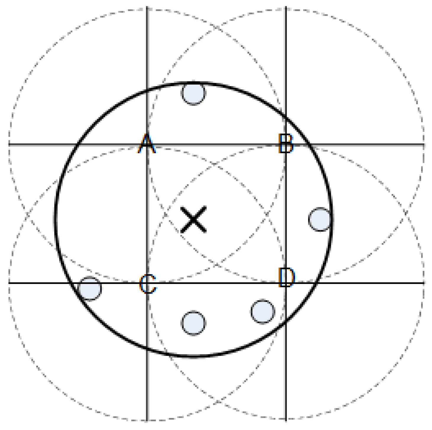
However, this approximation method may not find an optimal solution to the wireless communication tower placement problem, as the approximation method omits a large amount of continuous search space. Figure 1 shows a scenario where a discrete algorithm cannot find an optimal solution to a wireless communication tower placement problem. In this scenario, there are five users and four grid points, A, B, C, and D. However, if the wireless communication tower is placed at A, B, C, or D, the wireless communication tower cannot cover all five users. However, as illustrated in the figure, all five users can be covered by a single wireless communication tower at the location marked ‘×’. Since the location is not a grid point, this optimal solution is excluded by the approximation method.

Figure 1.
A scenario where a discrete algorithm cannot find an optimal solution. In this figure, users are marked with ‘∘’, A, B, C, and D are grid points where a wireless communication tower can be placed, the solid line circle represents the coverage of the wireless communication tower placed at marked ‘×’, and broken line circles are the coverage of the wireless communication tower placed at the grid points A, B, C and D.
In addition, most existing methods for discrete wireless communication tower placement problems use integer programming, mixed integer programming, or mixed integer nonlinear programming. Thus, they are suitable for large-scale communication tower placement problems, as they are not scalable.
In recent years, simulated annealing (SA) has been used to solve various tower/base station placement problems [25,26]. The research problem addressed in [25] is a discrete base transmitter station (BTS) problem. Its objectives are to optimize the capacity and location of existing BTS towers to obtain telecommunication efficiency and quality of service. The research problem addressed in [26] is a classical k-facility placement problem. It is also a discrete placement problem, as it is assumed that all the facilities must be placed on a grid graph. The objective is to maximize the coverage of k facilities.
This paper directly addresses the new continuous space wireless communication tower placement problem. Given a two-dimensional area, a list of users distributed in the area, and the number of wireless communication towers to be deployed in this area, the new continuous space wireless communication tower placement problem is to find a placement of the wireless communication towers in the area such that the total number of users that can be covered by the wireless communication network is maximal.
In this paper, we propose a hybrid simulated SA approach to the new continuous space wireless communication tower placement problem. To our knowledge, no other researcher has applied SA to any continuous wireless communication tower placement problem. In this paper, we model the continuous wireless communication tower placement problem as a continuous function optimization problem and solve it using a hybrid SA algorithm that capitalizes on the powerful exploration capability of SA and the efficient and effective exploitation capability of a local search procedure.
3. Problem Formulation
Given an area where a new wireless communication network will be deployed, a set of users of the new wireless communication network in the area, and the number of wire communication towers and the coverage of the communication towers, the new continuous space communication tower placement problem is to find a placement of those wireless communication towers such that the total number of users that can be covered by the wireless communication network is maximal.
This new continuous space wireless communication placement problem is formulated as follows:
- Given
- A two-dimensional continuous area, A, and a set of n users in A, , where are the coordinates of user and ;
- A set of m communication towers, ;
- The coverage of the communication towers, ;
- find
a placement of the m wireless communication towers , where is the coordinates of the tower and ,
- such that
is maximum, where is a set of users that can be covered by p. A user is said to be covered by p if there exists a communication tower such that the Euler distance between and is less than or equals to , that is, , where are the coordinates of , are the coordinates of in p, and is the coverage of the communication tower.
4. Hybrid Simulated Annealing Algorithm
SA, originally proposed by Kirkpatrick, Gelatt, and Vecchi [27] in 1983 and then by Černy in 1985 [28], has been applied to many optimization problems of different kinds. SA is a global optimization technique. It starts with an initial solution and performs global optimization by iteratively generating, evaluating, and selecting a new solution from the current solution with a controlled annealing schedule. At each step, SA considers a neighbor of the current solution and probabilistically decides whether the current solution should be replaced with the new solution using a probability-based acceptance strategy. Typically, this step is repeated until the search reaches a solution that is good enough for the application or until a given computation budget has been exhausted.
When applying conventional SA to the placement problem initially, we observed that its exploration capacity is powerful, but its local exploitation capacity is poor (this is discussed in the next section of this paper). Thus, we developed a hybrid SA that capitalizes on the powerful global exploration capability of the conventional SA and the effective and efficient exploitation capability of a local optimization algorithm. Algorithm 1 is a high-level description of the hybrid SA algorithm.
| Algorithm 1 Hybrid SA algorithm |
|
In the following, we discuss the details of the hybrid SA, including cost function, cooling schedule, neighbor generation, acceptance of a new solution, termination condition of the hybrid SA, and the local optimization algorithm.
4.1. Cost Function
The cost of a solution, P, is defined by Equation (1).
where is the total number of users and represents the total number of users that are covered by P.
When equals 0, P is an optimal solution to the wireless communication tower placement problem. It should be noted that when P is an optimal solution to a wireless communication tower placement problem, however, may not be equal to 0. In other words, is a sufficient condition, but it is not a necessary condition for P to be an optimal solution.
4.2. Cooling Schedule
4.3. Neighbor Generation
A neighbor of P is a new placement of the wireless communication towers that can be obtained by randomly changing the location of one randomly selected wireless communication tower in P.
4.4. Acceptance of a New Solution
If a new solution (neighbor) has a lower cost than the current solution P, then the current solution P is replaced by the new solution ; otherwise, P is replaced by with the probability determined by the acceptance function below:
where and are the cost of the new solution and the cost of the current solution P, respectively, t is the current time, and is the current temperature.
4.5. Termination Condition
The hybrid SA ends when or , where is the temperature at current time t, is a preset temperature and is the cost of the current wireless communication tower placement solution P.
4.6. Local Optimization
4.6.1. Motivation
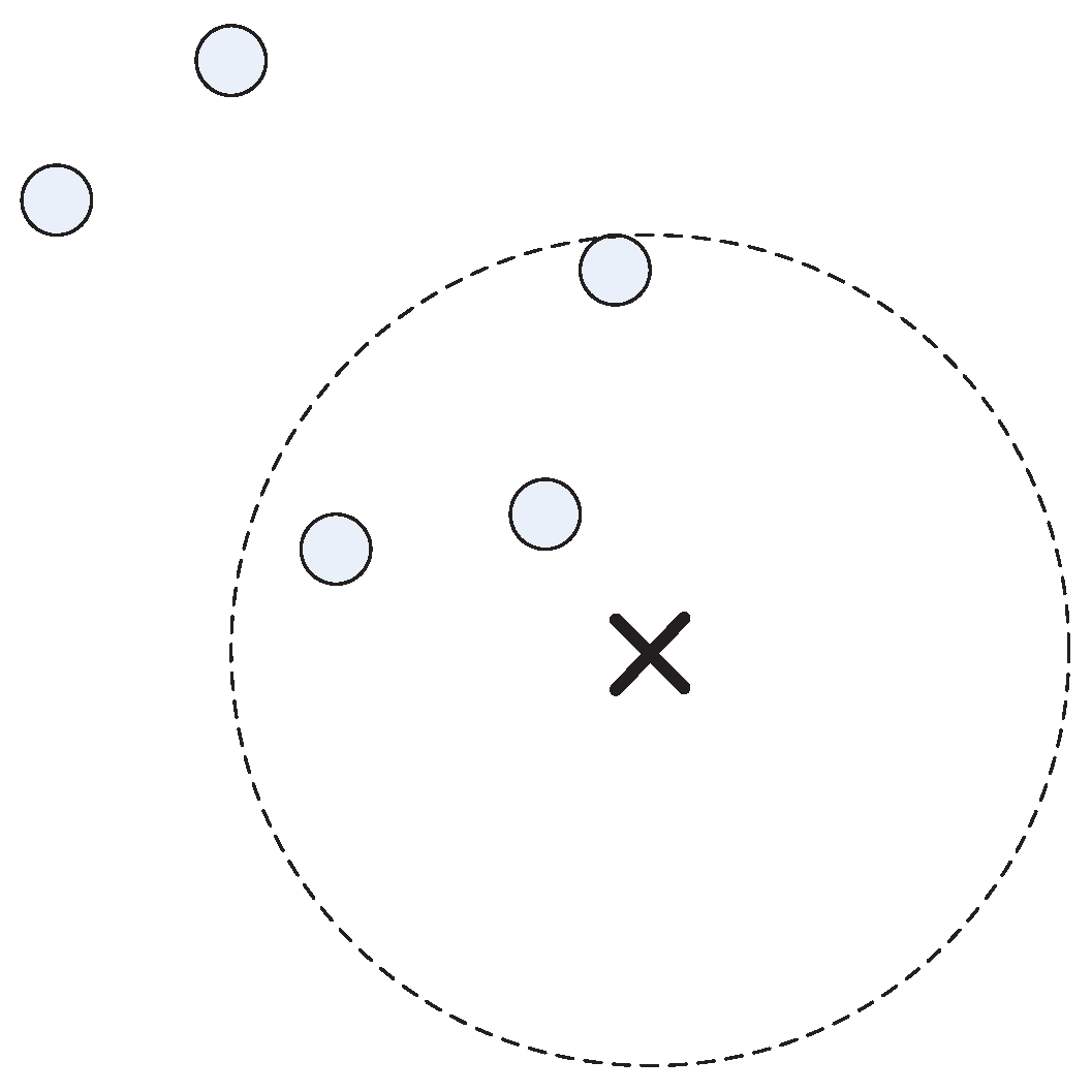
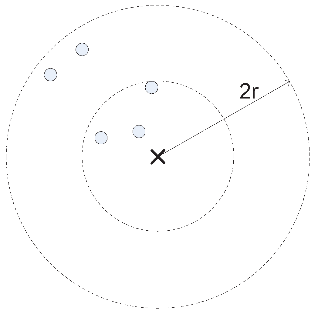
Initially, we developed a conventional SA algorithm for the wireless communication tower placement problem. However, when conducting experiments on the conventional SA, we observed that its exploration ability is great, but its exploitation ability is very poor, as in the process of annealing, the conventional SA could find an area where a number of users were clustered but could not find an optimal location for a wireless communication tower placement to cover maximally those users in the area. Figure 2 illustrates a typical solution found using the conventional SA algorithm.
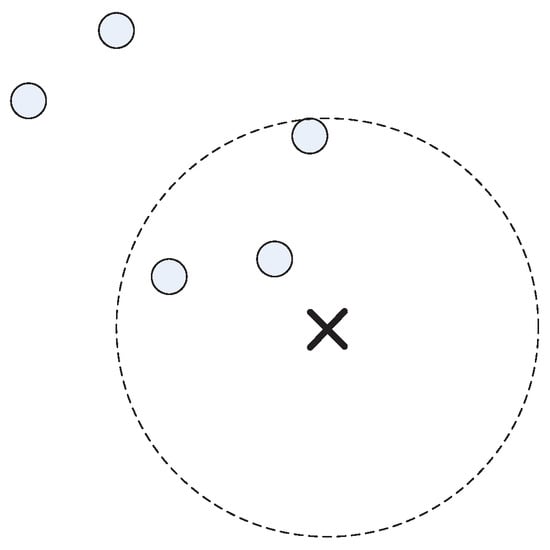
Figure 2.
A wireless communication tower location found by the conventional SA. In this figure, a user is marked by a ‘∘’, a wireless communication tower is represented by a ‘×’, and the coverage of a wireless communication tower is represented by a large broken line circle.
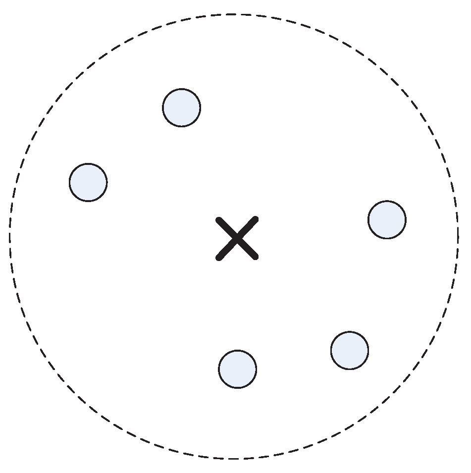
It can be seen from the figure that the conventional SA explored an area where five users are clustered. However, the solution found by the conventional SA algorithm covers only three of the five users. If we move the location of the wireless communication tower to the location illustrated in Figure 3, the wireless communication tower will cover all five users. This indicates that the exploitation capacity of the SA needs to be improved. Thus, it is desirable to develop a local optimization algorithm that can find an optimal or a near-optimal solution when the conventional SA algorithm explores a new search area. The local optimization algorithm can be embedded into the conventional SA to enhance the conventional SA’s local exploitation ability.
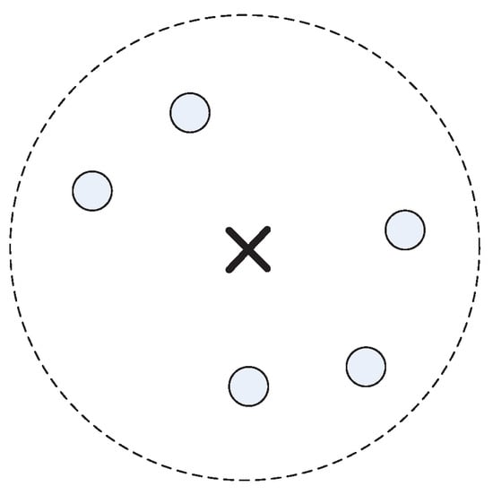
Figure 3.
The ideal location of the wireless communication tower.
4.6.2. Design of the Local Optimization Algorithm
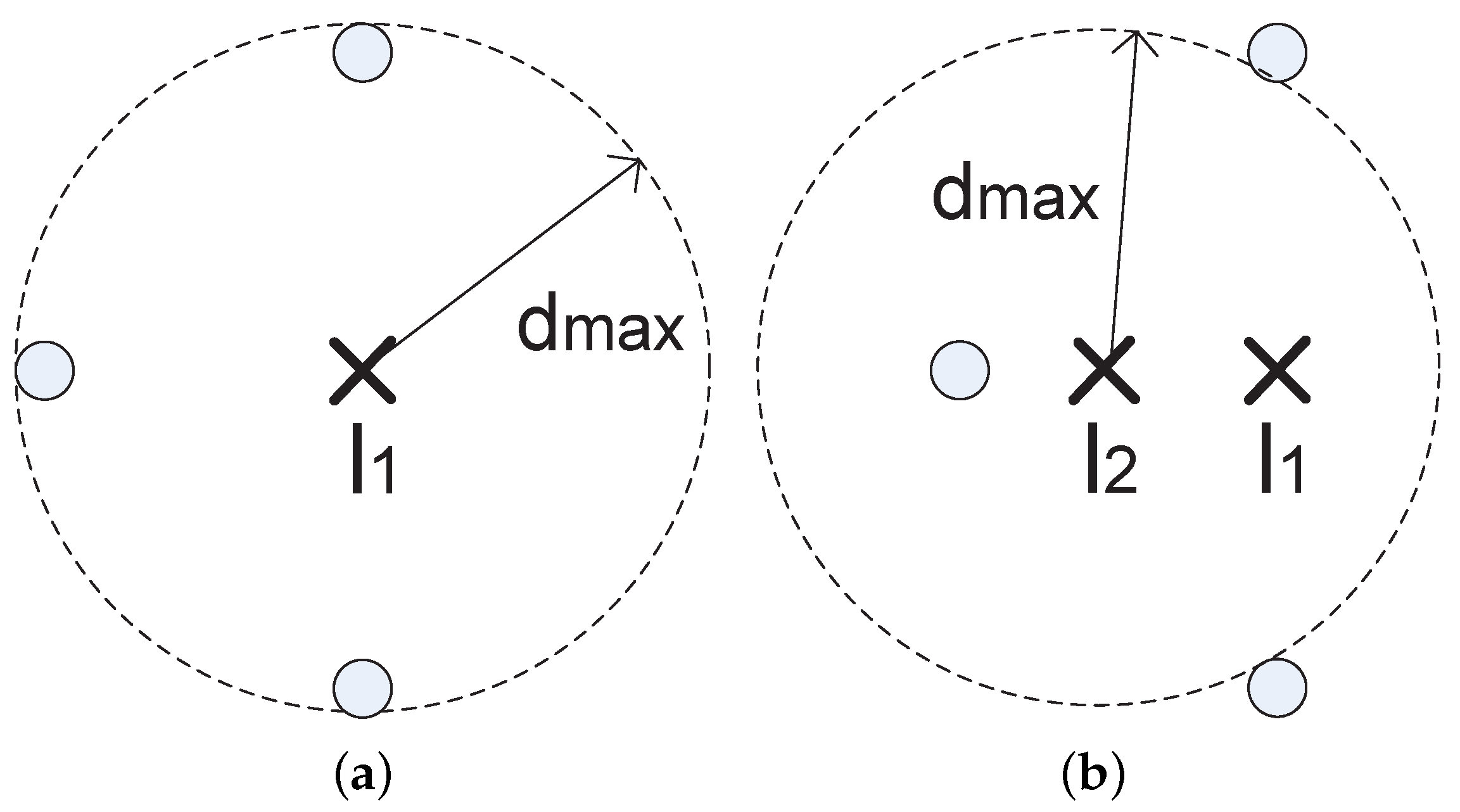
The basic ideas behind it are as follows: first, it searches for uncovered users that are close to the location of a wireless communication tower currently found by the SA; then, it relocates the wireless communication tower so that the wireless communication tower can cover more uncovered users, if possible. In order to find uncovered users that are close to a wireless communication tower, the local optimization algorithm finds all uncovered users in the radius of , which is a control parameter of the search. Experimental results have shown that when , the local optimization algorithm gives the best results. Figure 4 illustrates this idea.

Figure 4.
Search for uncovered users that are close to a wireless communication tower.
In order to find a new location to build a wireless communication tower to cover more users, we initially tried moving the wireless communication tower to the geographically central location of its covered users. However, this method did not work very well because sometimes, after moving the wireless communication tower to the geographical center, the number of covered users becomes smaller. Figure 5 shows this scenario. It can be seen that, in the new location, the wireless communication tower can cover only one user.

Figure 5.
Geographical center method. In this figure, (a) shows the initial location of the wireless communication tower, , in which the wireless communication tower can cover three users; (b) illustrates the situation where the wireless communication tower has been moved to the geographical center of the three users, .
From a computational perspective, this problem can be formulated as a so-called constrained maximum covering problem. Given a circle of radius and a set of points in the Euclidean plane, S, which are enclosed in the circle, and another set of points in the Euclidean plane, , the constrained maximum covering problem is to find a new enclosing circle of radius such that it encloses the maximum number of points in in addition to those points in S. We designed an algorithm to solve the constrained maximum coverage problem, as described in Algorithm 2.
| Algorithm 2 MaxCoverage(S, , ) |
|
The basic idea behind the constrained maximum enclosing circle algorithm is simple. It iterates times, and in each iteration, it randomly picks up a point p from and then uses the randomized algorithm for the minimum enclosing circle problem proposed by Emo Welzl [29] to find the minimum enclosing circle that encloses all points in S and the randomly selected point from , p. If the radius of the minimum enclosed circle is less than or equal to , we move the randomly selected point p from to S; if the radius of the minimum enclosing circle is greater than , then we remove the randomly selected point p from . After iterations, this algorithm finds a circle of radius that encloses the maximum number of points in in addition to those points in S.
Theorem 1.
The time efficiency of Algorithm 2 is .
Proof.
The while statement iterates times, and in each of the iterations, one user is removed from .
Assume that is implemented in a list. Thus, in the th iteration, it takes a constant time to obtain the last point p from and remove it from (steps 2 and 3); a time to find the minimum enclosing circle, as the MiniEnclCircle procedure has a linear time efficiency (step 4); a constant time to compute the radius of the minimum enclosing circle c, r (step 5); a time that is no more than to complete the if statement (steps 6–8). As a result, the total computation time of the th iteration of the while statement is no more than = , where , , , , and are constants.
Thus, the total computation time of the algorithm is
where .
Thus, the time efficiency of the algorithm is . □
Using this constrained maximum cover circle algorithm, we designed a local optimization algorithm. The input of this local optimization algorithm is a placement of a wireless communication tower , , ⋯, , where is the location of the th wireless communication tower in this wireless communication tower placement, , and m is the total number of wireless communication towers. The result of this local optimization is an optimized placement of the wireless communication tower. Algorithm 3 is the high-level description of the local optimization algorithm.
| Algorithm 3 Maximum coverage-based local optimization (P) |
|
The local optimization algorithm optimizes the location of wireless communication towers one by one using the constrained maximum cover circle algorithm. For each of the wireless communication tower locations r, the algorithm calculates all the users covered by r, stores them in S, and identifies all users that are not covered by r, but the distance from the location of r to the users is less than or equal to , putting these users in . Note that includes all potential users that can be covered by r by moving r to a new location without losing any user in S. Then, the algorithm uses the constrained maximum cover circle algorithm to find a new location for r where it can cover as many users in as possible in addition to all users in S.
Theorem 2.
The time efficiency of Algorithm 3 is , where is the number of users and is the set of wireless communication towers.
Proof.
For each wireless communication tower r, it takes a time to computer its S and (steps 2–14), and it takes a time to find a new location for r (step 15). Since and , the total computation time of each iteration is less than or equal to . Since there are wireless communication towers, the while loop iterates times. Thus, the time efficiency of the local optimization algorithm is . □
Theorem 3.
The time efficiency of Algorithm 1 is , where is the number of users, is the set of wireless communication towers, and l is the number of iterations that the algorithm executes.
Proof.
The basic operation in this algorithm is the local optimization procedure in Step 13. In the worst case, the procedure is invoked l times, where l is the number of iterations of the while loop. Since the time efficiency of the local optimization procedure is , the time efficiency of Algorithm 1 is l= in the worst case. □
5. Experimental Analysis
This section is devoted to the experimental analysis of the hybrid SA. In this section, we analyze the exploration and exploitation capacities of the hybrid SA, the effectiveness of the hybridization in the hybrid SA algorithm, and the performance and scalability of the hybrid SA.
There are two parameters in the HSA. One is the initial temperature ; the other is the lowest temperature , which is used in the termination condition. In this analysis of experiments, and . The values of the two parameters were obtained by experiments.
5.1. Exploration and Exploitation Capacities
The exploration capacity of a search algorithm is the capacity to discover new promising search regions, and the exploitation capacity of a search algorithm is the capacity to exploit the discovered promising regions. If the exploration capacity of a search algorithm is not powerful, then some promising search regions may be missed by the search algorithm, and therefore, it cannot find the region where the optimal solution is situated; if the exploitation capacity of a search algorithm is limited, then the search algorithm cannot find the optimal solution even if the search region where the optimal solution is situated is discovered by the search algorithm.
To evaluate the exploration and exploitation capacities of the hybrid SA, we generate a number of test problems whose promising search regions and optimal solutions are known (the generation of such test problems is discussed later in this section) and use the hybrid SA to solve the test problems. Thus, we know if all the promising search regions are explored and if the solutions are the optimal ones for those test problems. If the hybrid SA does not discover any of the promising search regions, then the exploration capacity of the hybrid SA is questionable; if the hybrid SA explores all the promising search regions of a problem but cannot find the optimal solution or a near-optimal solution, then the exploitation capacity of the hybrid SA is limited.
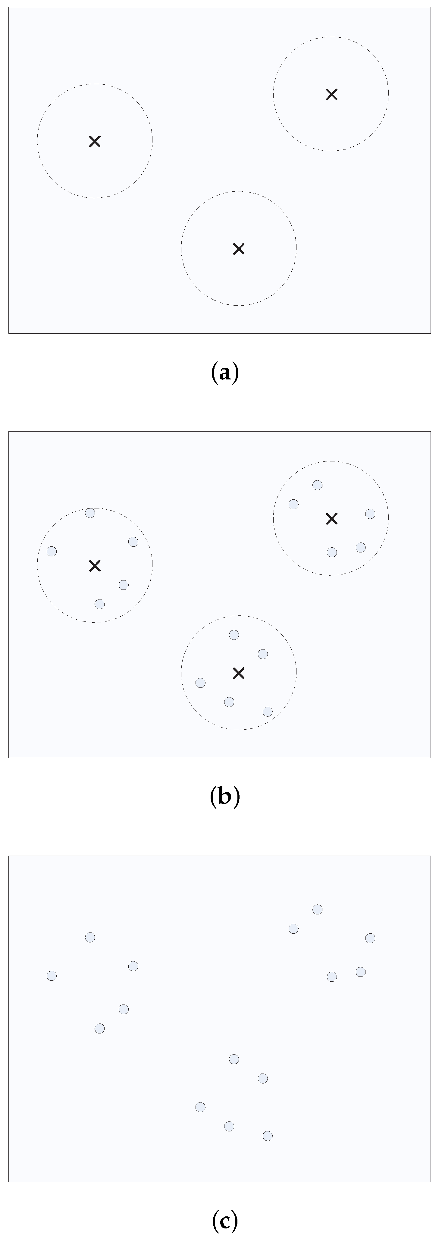
To generate a test problem with known promising search regions and the optimal solution, firstly, we randomly generate m wireless communication tower locations in a geographical area, making sure that the distance between any pair of wireless communication tower locations is greater than . In this way, we can guarantee that there will be no user that can be covered by more than one wireless communication tower. Secondly, for each of the wireless communication towers, we randomly generate k user locations surrounding it so that all users can be covered by the wireless communication tower. Thirdly, we remove those wireless communication tower locations and obtain a test problem with users and m wireless communication towers. The test problem is to find the locations of m wireless communication towers in the geographical area.
Figure 6 illustrates this test problem generation process where and . In the first step, we create three wireless communication tower locations, as shown in Figure 6a. Then, in the second step, we randomly generate five users surrounding each of the three wireless communication towers, as illustrated in Figure 6b. Finally, in the third step, we remove the three wireless communication towers and obtain a test problem, as shown in Figure 6c.
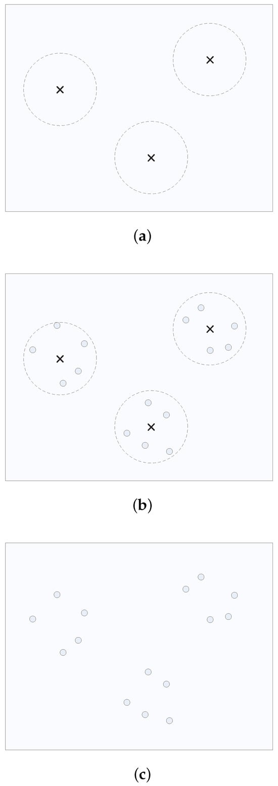
Figure 6.
The process of generating a wireless communication tower placement problem with known promising regions and an optimal solution. In the figure, ‘×’ represents the location of a wireless communication tower, and ‘∘’ stands for the location of a user, and a large broken line circle shows the coverage of a wireless communication tower.
The number of wireless communication towers in a test problem gives the number of promising search areas. In a test problem generated in this way, the users are clustered around the randomly generated wireless communication tower locations. Thus, if an algorithm can reach at least one user from each of the user clusters, the algorithm’s exploration capacity is excellent, as it explores all the promising search areas of the problem. Let us say that the number of wireless communication towers is m and the number of users is k. Then, if the algorithm can find or more users, then it explores all the promising search areas of the test problem. To evaluate the exploitation capacity of an algorithm, we look at the total number of users that are covered in a solution generated by the algorithm in a promising area.
It can be seen from the test problem shown in Figure 6c that the users are clustered in three regions, which are three promising regions to which the hybrid SA should reach; otherwise, the hybrid SA will not find the optimal or near-optimal solution for the test problem. If the hybrid SA finds a solution that does not cover any user in any of the three regions, then we know that the hybrid SA did not explore all the promising regions and, therefore, its exploration capacity is of concern. If the hybrid SA finds a solution that covers at least one user in each of the regions but does not cover all or the majority of the users in the regions, then we know the hybrid SA explores all the promising regions but cannot exploit well in the regions. If the hybrid SA can find the optimal or a near-optimal solution for the test problem, then it indicates that both the exploration capacity and the exploitation capacity of the hybrid SA are fine.
Using the aforementioned test problem generation ideas, we developed a program and used it to randomly generate two classes of test problems. In one class of test problems, the number of wireless communication towers was fixed at 10, but the number of users in the test problems ranged from 100 to 1000 with increments of 100. In the other class of test problems, the number of users was fixed to 500, but the number of wireless communication towers varied from 10 to 100 with increments of 10. Parameter was set to 70 in all test problems. The reasons for generating the two classes is that the size of a test problem depends on both the number of wireless communication towers and the number of users and we are interested in how the computation time of the hybrid SA increases when the number of wireless communication towers increases and how the computation increases when the number of users grows in addition to the exploration and exploitation capacities of the hybrid SA.
For each of the parameter configurations, we randomly generated 30 different instances in order to make sure that the experimental results were statistically significant, and for each of the instances, we used the hybrid SA algorithm to solve it. The ratio of the number of users covered by the wireless communication towers in the solution generated by the hybrid SA and the total number of users, namely, coverage rate, was recorded. The coverage rate indicates both the exploration capacity and the exploitation capacity of a search algorithm.
Table 1 shows the statistics of the experimental results for the two classes of test problems. The top 10 rows in the table show the statistics of the experimental results for the first class of test problems, and the bottom 10 rows show the statistics for the experimental results of the second class of test problems. Each row shows the statistics of 30 runs for 30 different test problems with the same configuration. The total number of test problems was 600.

Table 1.
Statistics of the experimental results on the exploration and the exploitation capacities of the hybrid SA.
It can be seen from Table 1 that, among the 600 tests, the hybrid SA found an optimal solution for the test problem and that, in the worst scenario, the hybrid SA still found a solution with a coverage ratio of 0.96. Thus, it can be concluded that both the exploration capacity and the exploitation capacity of the hybrid SA are excellent, as the hybrid SA explored all the promising search areas for each of the test problems and found almost all the users in each of the promising regions.
5.2. Effectiveness of the Hybridization
The hybrid SA is the hybridization of conventional SA and a local optimization algorithm. To examine the effectiveness of the hybridization, we simply compare the performance of the conventional SA with the local optimization algorithm, i.e., the hybrid SA, to that of the conventional SA without the local optimization algorithm using those test problems that were used for evaluating the exploration and exploitation capacities of the hybrid SA previously.
For each of the test problems, we used the two SA algorithms to solve them. The quality of the solutions (coverage rate) was recorded. Considering the stochastic nature of the two SA algorithms, we performed each experiment 30 times. Table 2 shows the statistics of the experimental results.
Table 2.
Statistics of the experimental results on the conventional SA and the hybrid SA for random test problems.
It can be seen from the statistics of the experimental results that the hybrid SA algorithm (the SA with the local optimization algorithm) found an optimal solution for all the test problems in the 30 runs. In fact, it found an optimal solution in most of the 30 runs for every test problem. On the contrary, the conventional SA algorithm (the SA without the local optimization algorithm) never found an optimal solution to any test problem in any run. The average coverage rate of the wireless communication tower placement solutions found by the hybrid SA algorithm for the test problems is between 0.993 and 1.000, whereas the average coverage rate of the wireless communication tower placement solutions found by the conventional SA for the same test problems is only between 0.741 and 0.806. In other words, the hybrid SA algorithm could always find an optimal or near-optimal solution, but the conventional SA could not. Since the only difference between hybrid SA and conventional SA is whether they use the hybridization technique or not, the experimental results show that the hybridization technique is effective.
5.3. Scalability
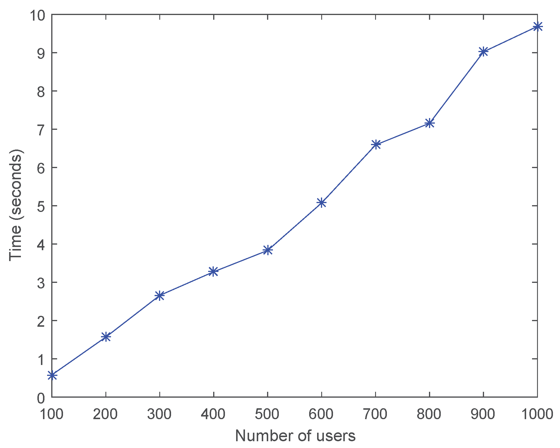
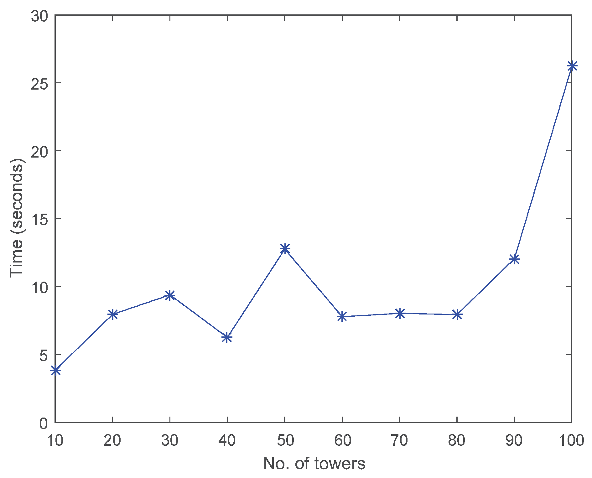
To test the scalability of the hybrid SA, we check if the hybrid SA can find an optimal or near-optimal solution in a reasonable time when the problem size increases. In previous experiments, we also recorded the computation time of the hybrid SA algorithm for each of the test problems. Figure 7 shows how the computation time of the hybrid SA algorithm increases linearly as the number of potential users increases. Figure 8 shows how the computation time of the hybrid SA algorithm also increases linearly as the number of wireless communication towers increases, although there are some skews in the curve. All experiments were conducted on a desktop computer with an Intel Core 2 Duo CPU of 3.00 GHz and 4.00 GB RAM. It can be seen from the figure that the time efficiency of the hybrid SA is bounded by , where n is the total number of users. Thus, it can be concluded that the hybrid SA is scalable.
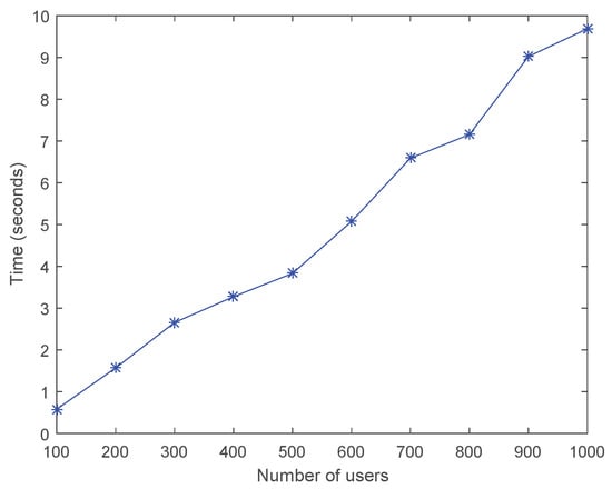
Figure 7.
The computation time with respect to the number of users.
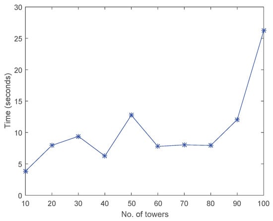
Figure 8.
The computation time with respect to the number of wireless communication towers.
6. Conclusions and Discussion
In this paper, we identify a new emerging communication tower placement problem and formulate the continuous communication tower placement problem as a continuous function optimization problem. We also propose a hybrid SA algorithm for the new communication tower placement problem. The hybrid SA algorithm employs the powerful exploration capability of SA to explore the continuous search space and enhances its local exploitation capability by incorporating an effective local optimization procedure. In addition, in this paper, we demonstrate through experiments the effectiveness of the hybridization, the performance, and the scalability of the hybrid SA.
In this paper, we focus on the core of the new communication tower placement. The hybrid SA algorithm can be extended to handle pre-deployed communication towers by simply removing users that have already been covered by those pre-deployed communication towers before applying the hybrid SA algorithm to solve the wireless communication tower placement problem. It can also be extended to consider the situation in which there exist sites that are not suitable for placing a communication tower, such as ponds, by not accepting any new neighbor (new solution) in which there exists a communication tower that is located at a place where a communication tower cannot be deployed.
Finally, the local optimization algorithm is not specific to this hybrid SA. It can be used in other continuous space communication tower placement algorithms to further improve the quality of their solutions.
Author Contributions
Individual contributions: conceptualization, M.T. and W.L.; design of experiments, M.T. and W.L.; implementation of experiments, M.T.; analysis of experimental results, M.T.; original draft preparation, M.T.; writing—review and editing, M.T. and W.L. All authors have read and agreed to the published version of the manuscript.
Funding
This research received no external funding.
Data Availability Statement
The data presented in this study are available in this article.
Conflicts of Interest
The authors declare no conflicts of interest.
References
- Hassana, G.; Liu, Y.; Hakim, G.; Drissa, K. 5G base station deployment perspectives in millimeter wave frequencies using meta-heuristic algorithms. Electronics 2019, 8, 1318. [Google Scholar] [CrossRef]
- Tang, M. A memetic algorithm for the location-based continuously operating reference stations placement problem in network real-time kinematic. IEEE Trans. Cybern. 2015, 45, 2214–2223. [Google Scholar] [CrossRef] [PubMed]
- Houssein, E.H.; Saad, M.R.; Hussain, K.; Zhu, W.; Shaban, H.; Hassaballah, M. Optimal Sink Node Placement in Large Scale Wireless Sensor Networks Based on Harris’ Hawk Optimization Algorithm. IEEE Access 2020, 8, 19381–19397. [Google Scholar] [CrossRef]
- Wright, M.H. Optimization methods for base station placement in wireless applications. In Proceeding of the 48th IEEE Vehicular Technology Conference, Ottawa, ON, Canada, 21 May 1998; pp. 387–391. [Google Scholar]
- Weicker, N.; Szabo, G.; Weicker, K.; Widmayer, P. Evolutionary multiobjective optimization for base station transmitter placement with frequency assignment. IEEE Trans. Evol. Comput. 2003, 7, 189–203. [Google Scholar] [CrossRef]
- Wong, J.K.L.; Mason, A.J.; Neve, M.J.; Sowerby, K.W. Base station placement in indoor wireless systems using binary integer programming. IEEE Proc. Commun. 2006, 153, 771–778. [Google Scholar] [CrossRef]
- Aldajani, M.A. Convolution-based placement of wireless base stations in urban environment. IEEE Trans. Veh. Technol. 2008, 57, 3843–3848. [Google Scholar] [CrossRef]
- Yang, D.; Misra, S.; Xue, G. Joint base station placement and fault-tolerant routing in wireless sensor networks. In Proceedings of the IEEE GLOBECOM, Honolulu, HI, USA, 30 November–4 December 2009; pp. 1–6. [Google Scholar]
- Bor-Yaliniz, R.I.; El-Keyi, A.; Yanikomeroglu, H. Efficient 3-d placement of an aerial base station in next generation cellular networks. In Proceedings of the IEEE ICC, Kuala Lumpur, Malaysia, 22–27 May 2016; pp. 1–5. [Google Scholar]
- Wang, Q.; Xu, K.; Takahara, G.; Hassanein, H. Device placement for heterogeneous wireless sensor networks: Minimum cost with lifetime constraints. IEEE Trans. Wirel. Commun. 2007, 6, 2444–2453. [Google Scholar] [CrossRef]
- Lin, B.; Ho, P.-H.; Xie, L.-L.; Shen, X.; Tapolcai, J. Optimal relay station placement in broadband wireless access networks. IEEE Trans. Mob. Comput. 2010, 9, 259–269. [Google Scholar] [CrossRef]
- Dhillon, S.S.; Chakrabarty, K. Sensor placement for effective coverage and surveillance in distributed sensor networks. In Proceedings of the IEEE WCNC 2003, New Orleans, LA, USA, 16–20 March 2003; pp. 1609–1614. [Google Scholar]
- Cheng, X.; Du, D.Z.; Wang, L. Relay sensor placement in wireless sensor networks. Wirel. Netw. 2008, 14, 347–355. [Google Scholar] [CrossRef]
- Ling, X.; Yeung, K.L. Joint access point placement and channel assignment for 802.11 wireless LANs. IEEE Trans. Wirel. Commun. 2006, 5, 2705–2711. [Google Scholar] [CrossRef]
- Sarkar, S.; Yen, H.-H.; Dixit, S.; Mukherjee, B. Hybrid wireless-optical broadband access network (WOBAN): Network planning using lagrangean relaxation. IEEE/ACM Trans. Netw. 2009, 17, 1094–1105. [Google Scholar] [CrossRef]
- Yin, H.; Zhang, X.; Luo, H.L.Y.; Tian, C.; Zhao, S.; Li, F. Edge provisioning with flexible server placement. IEEE Trans. Parallel Distrib. Syst. 2017, 28, 1031–1045. [Google Scholar] [CrossRef]
- Li, Y.; Wang, S. An energy-aware edge server placement algorithm in mobile edge computing. In Proceedings of the IEEE EDGE, San Francisco, CA, USA, 2–7 July 2018; pp. 66–73. [Google Scholar]
- Jia, M.; Cao, J.; Liang, W. Optimal cloudlet placement and user to cloudlet allocation in wireless metropolitan area networks. IEEE Trans. Cloud Comput. 2017, 5, 725–737. [Google Scholar] [CrossRef]
- Mondal, S.; Das, G.; Wong, E. Ccompassion: A hybrid cloudlet placement framework over passive optical access networks. In Proceedings of the IEEE INFOCOM, Honolulu, HI, USA, 16–19 April 2018; pp. 216–224. [Google Scholar]
- Yang, S.; Li, F.; Shen, M.; Chen, X.; Fu, X.; Wang, Y. Cloudlet placement and task allocation in mobile edge computing. IEEE Internet Things J. 2019, 6, 5853–5863. [Google Scholar] [CrossRef]
- Aoun, B.; Boutaba, R.; Iraqi, Y.; Kenward, G. Gateway placement optimization in wireless mesh networks with QoS constraints. IEEE J. Sel. Areas Commun. 2006, 24, 2127–2136. [Google Scholar] [CrossRef]
- Li, P.; Huang, X.; Fang, Y.; Lin, P. Optimal placement of gateways in vehicular networks. IEEE Trans. Veh. Technol. 2007, 56, 3421–3430. [Google Scholar] [CrossRef]
- Guo, J.; Rincón, D.; Sallent, S.; Yang, L.; Chen, X.; Chen, X. Gateway placement optimization in leo satellite networks based on traffic estimation. IEEE Trans. Veh. Technol. 2021, 70, 3860–3876. [Google Scholar] [CrossRef]
- Tang, M. Evolutionary placement of continuously operating reference stations of network real-time kinematic. In Proceedings of the IEEE CEC, Brisbane, QLD, Australia, 10–15 June 2012; pp. 1–8. [Google Scholar]
- Firli, A.; Primiana, I.; Kaltum, U.; Oesman, Y.M.; Herwany, A.; Azis, Y.; Yunani, A. CAPEX efficiency and service quality improvement via tower sharing in the Indonesian telecommunication industry: Optimisation model using comparison of genetic algorithm and simulated annealing methods. Int. J. Serv. Econ. Manag. 2017, 8, 90–108. [Google Scholar] [CrossRef]
- Coll, N.; Fort, M.; Saus, M. Coverage area maximization with Parallel Simulated Annealing. Expert Syst. Appl. 2022, 202, 117185. [Google Scholar] [CrossRef]
- Kirkpatrick, S.; Gelatt, C.D., Jr.; Vecchi, M.P. Optimization by simulated annealing. Science 1983, 220, 671–680. [Google Scholar] [CrossRef]
- Černý, V. Thermodynamical approach to the problem of traveling salespeople: An efficient simulation algorithm. J. Optim. Theory Appl. 1985, 45, 41–51. [Google Scholar] [CrossRef]
- Welzl, E. Smallest enclosing disks (balls and llipsoids). Lect. Notes Comput. Sci. 1991, 555, 359–370. [Google Scholar]
Disclaimer/Publisher’s Note: The statements, opinions and data contained in all publications are solely those of the individual author(s) and contributor(s) and not of MDPI and/or the editor(s). MDPI and/or the editor(s) disclaim responsibility for any injury to people or property resulting from any ideas, methods, instructions or products referred to in the content. |
© 2024 by the authors. Licensee MDPI, Basel, Switzerland. This article is an open access article distributed under the terms and conditions of the Creative Commons Attribution (CC BY) license (https://creativecommons.org/licenses/by/4.0/).