A Microservices-Based Control Plane for Time-Sensitive Networking

Abstract

Time-Sensitive Networking (TSN) aims to provide deterministic communications over Ethernet. The main characteristics of TSN are bounded latency and very high reliability, thus complying with the strict requirements of industrial communications or automotive applications, to name a couple of examples. In order to achieve this goal, TSN defines several scheduling algorithms, among them the Time-Aware Shaper (TAS), which is based on time slots and Gate Control Lists (GCLs). The configuration of network elements to allocate time slots, paths, and GCLs is laborious, and has to be updated promptly and in a dynamic way, as new data flows arrive or disappear. The IEEE 802.1Qcc standard provides the basis to design a TSN control plane to face these challenges, following the Software-Defined Networking (SDN) paradigm. However, most of the current SDN/TSN control plane solutions are monolithic applications designed to run on dedicated servers, and do not provide the required flexibility to escalate when facing increasing service requests. This work presents $\mu$TSN-CP, an SDN/TSN microservices-based control plane, based on the 802.1Qcc standard. Our architecture leverages the advantages of microservices, enabling the control plane to scale up or down in response to varying workloads dynamically. We achieve enhanced flexibility and resilience by breaking down the control plane into smaller, independent microservices. The performance of $\mu$TSN-CP is evaluated in a real environment with TSN switches, and various integer linear problem solvers, running over different computing platforms.

1. Introduction

Time Sensitive Networking (TSN) refers to a set of IEEE 802.1 standards that aim to provide deterministic, low-latency, and highly reliable communications over the existing Ethernet. TSN enables applications with different time-criticality levels to share transmission resources in Ethernet while meeting their latency, bandwidth, and reliability requirements [1].

One of the main standards of TSN is IEEE 802.1Qbv, which defines the Time-Aware Shaper (TAS). The TAS establishes Gate Control Lists (GCLs) for each outgoing port of the TSN switches to control which traffic classes can be transmitted at different time intervals. This feature ensures that traffic classes can access the transmission medium in a time-triggered manner, preventing non-critical traffic classes from invading the time slots assigned to time-critical traffic classes and, thereby, achieving bounded end-to-end latency [2]. The TAS requires precise time synchronization among all the nodes of a TSN domain (i.e., end stations and TSN switches). This synchronization is achieved with the Precision Time Protocol (PTP) by using the IEEE 802.1AS standard [3].

The assignment of time slots requires the TAS to know the network topology and the requirements of the different data streams, which end stations demand via the User/Network Interface (UNI). The IEEE 802.1Qcc standard defines three architecture models for getting the topology and user/network requirements and configuring the underlying network switches accordingly: the fully distributed model, the centralized network/distributed user model, and the fully centralized model. This work focuses on the fully centralized approach, which follows an SDN architecture, by removing the control logic from the network devices and allocating it in two entities: the Centralized Network Configuration (CNC) and the Centralized User Configuration (CUC).

Even though the IEEE 802.1Qcc standard defines the basis for implementing the fully centralized model, it includes general guidelines and does not provide concrete specifications. In the literature, several works have described centralized control planes for TSN [1,4,5,6]; however, these solutions follow non-scalable monolithic architectures, which are unable to allocate additional resources to specific tasks as needed. Such TSN control plane (CP) implementations consume significant computational resources and increase the time invested to calculate schedules, which consist of determining the length and position of time slots assigned to different GCLs at the outgoing ports of the TSN switches along network paths.

The concept of microservices is a promising approach to deal with the scalability issues of monolithic TSN CPs. Microservices are an architectural model that divides a monolithic application into different components, each one with a specific functionality [7]. Since these components are smaller than the whole monolithic application, it is easier to add or remove microservice instances [8], enabling resource allocation to highly demanded tasks more efficiently. In the literature, some works use microservices for SDN controllers: in [9], the authors create a cloud-native SDN controller based on the concept of microservices in the context of transport, while the work in [10] explores the use of microservices for a CP for open optical networks.

In this paper, we describe $\mu$TSN-CP [11], a microservice-based SDN CP architecture for TSN capable of retrieving network topology and stream requirements, calculating valid schedules, and configuring switches accordingly by optimizing the associated resource usage. Considering the CP’s atomic functionalities, $\mu$TSN-CP decomposes the CNC and CUC elements into microservices. Moreover, we implement a prototype of the $\mu$TSN-CP elements and analyze its performance on a hybrid cloud running on Amazon Web Services (AWSs) that use Docker and local instances. We focus on testing the ILP, which we provide as an example of a high-demand microservice in terms of computation, in order to analyze the qualitative characteristics that improve the computational resource usage (i.e., CPU and RAM) and the time spent calculating schedules.

The remainder of the paper is structured as follows. Section 2 describes related work. Section 3 describes the $\mu$TSN-CP architecture. Section 4 presents some experiments done to show the overall functionality of our platform, including a discussion of the quantitative results. Section 5 provides a qualitative discussion of the advantages of using the microservices architecture. The paper ends with the conclusions and the description of lines of future inquiry.

2. Related Work

Several works have addressed the design of a TSN CP based on the fully centralized model of the IEEE 802.1Qcc standard. The authors of [4] offer an SDN CP for FPGA TSN networks that includes a time-sensitive management protocol and a time-sensitive switching model. However, that contribution resorts to a protocol for the management of the underlying network that is different from the one described in the IEEE 802.1Qcc standard (which uses RESTCONF and NETCONF). RESTCONF [12] is an HTTP-based protocol used to manage information defined by YANG data models, encoded with JSON, while NETCONF [13], which is very similar to RESTCONF, is established over SSH and its messages are encoded in XML. Additionally, all the elements of the TSN CP are merged into a monolithic element, which limits the scalability and flexibility of the architecture. In [5], the authors leverage SDN and Object Linking and Embedding for Process Control Unified Architecture (OPC-UA) to build an SDN/TSN CP. In their implementation, they propose four elements (User Registration, Service Registration, Stream Management Component, and an OpenDaylight SDN Controller), where each element is running on a different computer. Even though this solution shows a certain degree of platform independence and is not completely monolithic, the authors do not exploit all the potential advantages of a microservice architecture. Furthermore, the Stream Management Component, in particular, performs several tasks that could be split further into separate microservices. Finally, in [14], the authors describe their intention to develop an open-source CUC that makes use of the OPC-UA protocol to communicate with the end devices, as well as RESTCONF and YANG structures to exchange information with the CNC in the UNI interface. As of the time of writing this paper, this project is only available to OPC Foundation members.

On the other hand, the concept of microservices is used in the literature for the design of SDN controllers. The authors of [9] propose $\mu$ABNO (Application-based Network Operations); this SDN architecture is based on microservices and achieves auto-scalability while enabling cloud-scale traffic load management. They use Kubernetes to orchestrate the containers that execute the microservices and a cloud-native architecture running on the Adrenaline Testbed platform. In [10], the authors build an SDN controller for open optical networks based on microservices. They rely on a microservices architecture with Docker containers and Kubernetes to enable platform-as-a-service network control, with automated and on-demand deployment of SDN controllers or applications, and on-the-fly upgrades or swaps of the software components.

In summary, most of the existing approaches present a monolithic design that fails to achieve good scalability and flexibility to accommodate varying traffic demands and wastes significant computational resources. In contrast, the $\mu$TSN-CP architecture addresses this issue by distributing the main CNC and CUC functionalities described in the IEEE 802.1 Qcc among microservices. This approach allows the system to escalate the resources needed for just the necessary functions upon changing traffic demands.

To the best of our knowledge, the only work that is similar to $\mu$TSN-CP is OpenCNC [15], a TSN control plane based on microservices. One of the differences is the use of gNMI in OpenCNC, while $\mu$TSN-CP uses the RabbitMQ message broker. Therefore, OpenCNC requires an additional microservice that adapts gNMI requests to NETCONF, to be able to configure TSN switches. Another remarkable difference is the use of the ONOS SDN controller by OpenCNC instead of OpenDaylight (used by $\mu$TSN-CP) in order to interact with the network switches and configure them. Although the description that can be found in OpenCNC’s software repository (as of December 2023) mentions the possibility of using an external Integer Linear Programming (ILP) solver, it describes a “fallback mechanism” that applies a hardcoded schedule, which does not take into account the established streams nor their characteristics and, hence, does not perform any optimization (it is merely a YAML file indicating cycle time and the percentages of the cycle assigned to each traffic class) [16]. Instead, our work already includes an ILP module which will be tested in the following sections. Finally, ref. [17] provides some results related to the performance evaluation of an automated TSN end station configuration platform that includes OpenCNC as one of its modules, but, to the best of our knowledge, there does not exist any published work focused on describing the performance of OpenCNC or any other TSN control plane based on microservices. In contrast, we tested different ILP solvers, running over different computing platforms (including local machines and cloud environments), to evaluate the performance of $\mu$TSN-CP.

3. μTSN-CP Architecture

This section starts with a general description of the architecture of the platform, and then provides more details about each one of its microservices.

3.1. Introduction

The general structure of $\mu$TSN-CP is shown in Figure 1. We now describe the typical flow of execution of events. First, whenever an end station (talker) wants to send a data flow to another end station (listener), the talker notifies the Centralized User Configuration (CUC), which collects the characteristics and the latency requirements of the streams, and passes this information to the CNC. Within the CNC, the TSN Controller receives the information about the requested data streams from the CUC via the UNI by means of RESTCONF. The scheduler determines a configuration of the switches (ingress and egress ports, timeslots) that complies with the requirements of the data streams according to the network topology information received from the SDN Controller through RESTCONF. Once the configuration is ready, the SDN Controller distributes the configuration commands to the switches via NETCONF and YANG models. The switches execute the configuration and the data flow sent from the talker is treated accordingly.

Regarding the microservice architecture, Figure 2 illustrates the microservices created for mapping the control plane (CP) functions in the CNC, as well as the communication tools and interfaces between them. Following the same typical flow of events described earlier, the Jetconf [18] microservice gathers the data stream information from the CUC and sends it to the Preprocessing microservice. This block combines the stream information with the topology information (received from the Topology Discovery function), and sends it to the scheduler (ILP Calculator). The configuration resulting from the scheduler is sent to the Southconf microservice, which forwards it to the OpenDaylight SDN Controller. This element is responsible for configuring the TSN switches (via NETCONF) accordingly, so as to satisfy the time constraints of the data flows.

The following subsections describe the functionalities of each microservice.

3.2. Jetconf Microservice

The Jetconf microservice is the point of contact between the CUC and the CNC, implementing the UNI interface with the YANG model defined in the IEEE 802.1Qcc standard [19]. This microservice handles the communication of the user requirements to the CNC internal microservices. As input, this microservice gets the JSON payload by means of a REST/API using RESTCONF, and such payload must match the definitions of the parameters in the YANG module. Some parameters included in the payload are the number of streams and the communication period, maximum latency, size, and smallest and highest transmission offsets. Considering such requirements, we decided to use Jetconf, an implementation of the RESTCONF protocol, as a base for the microservice [18].

In the output, this microservice should communicate the answer to the requested payload to the CUC; such output needs to include the feasibility of the communication as a binary value and the offset that each talker should follow to achieve the communication. Additionally, Jetconf should send the requested information in a JSON payload using the appropriate RabbitMQ queue (Jet-pre queue in Figure 3) to the Preprocessing microservice. Regarding security, Jetconf includes HTTP/2 over TLS certificated-based authentication to the clients; such certificates should be shared with the client (CUC) to grant the communication appropriately. Figure 3 depicts the general operation of the Jetconf microservice.

3.3. Topology Discovery Microservice

The Topology Discovery microservice is in charge of collecting the topology of the TSN network and providing it to the other microservices represented as a network matrix. For this task, this microservice uses LLDP [20], a data-link layer protocol used for advertising the network elements’ identity, capabilities, and adjacency. In a nutshell, the Topology Discovery microservice generates a list of all the available devices in the network by accessing them through SSH and retrieving their LLDP information. We combined bash scripts and Python3 to create this microservice, specifically using the Paramiko [21] library, which implements the SSHv2 protocol. Figure 4 shows the general architecture of this microservice and its parts.

What follows is a summary of the steps followed from the moment we start the communication to the moment the information is retrieved from the devices and parsed to the Preprocessing microservice:

• The Topology Generator module activates the retrieval of the topology information using the Paramiko module. It uses Paramiko to send commands to every device in the network to get the adjacency information of each device. Raw data is collected and stored as files in the microservice.
• The Topology Generator module gets all the files, cleans the information and translates it into a Network Topology Matrix.
• Once the network information is ready, the Topology Discovery microservice generates a JSON message in the RabbitMQ queue and sends it to the Preprocessing microservice.

3.4. Preprocessing Microservice

This microservice is the entry point of the data provided by the Topology Discovery and Jetconf microservices. In Figure 5, we can see the values that enter the Preprocessing microservice from those microservices. These input values are retrieved from their respective RabbitMQ queues. Two modules implement the functionalities of the microservice. The first one is the Dijkstra module, which uses the Dijkstra algorithm to determine the shortest path from origin to destination for the routes in the schedule. It is important to highlight that, in our $\mu$TSN-CP, the module for calculating the path from sources to destinations and the module for calculating the schedule are in different microservices, as seen in other sections. This design decision enables us to easily adapt the microservice to use other algorithms to calculate the path for the requested streams (e.g., Floyd–Warshall or Johnson’s algorithms).

The other primal functionality of the Preprocessing microservice is to adapt the parameters that are passed to the main microservice in the architecture, the ILP Calculator. This preprocessing job is necessary to reduce the number of tasks assigned to the ILP Calculator. As Figure 5 depicts, the delivered parameters correspond to values resultant from the Dijkstra module and the preceding microservices. Besides, maintaining specific functionalities in that microservice enhances the possibility of using different approaches implemented as a microservice instead of the ILP Calculator, simply following the black-box design criterion and respecting the inputs and outputs. Finally, as in the previous cases, the way to communicate the results to the ILP Calculator microservice is via a RabbitMQ queue.

3.5. ILP Calculator Microservice

The ILP Calculator microservice is in charge of the Integer Linear Programming (ILP) solver. ILP is a mathematical optimization and feasibility programming method in which a set of constraints (represented as linear inequalities) and a linear optimization function describe a problem [22]. The variables used in the definition of the linear constraints create a space of solution that is filled with the set of possible solutions that respect the constraints. The larger the number of variables and constraints are, the more complex the solution space is and the harder it is to get a solution to the scheduling problem. In $\mu$TSN-CP, all of the characteristics of the TAS scheduler are included in the mathematical model. We have adopted the ILP model described in [2], considering the values of ${\mathrm{c}}_1=1$ and ${\mathrm{c}}_2=0$ in the objective function, thus taking into account only the optimization of the excess queues.

In an ILP program, there are two pieces, namely the model itself (implemented with Python3 using Pyomo [23], in our case) and the mathematical solver (installed in the same Docker container as the model). There is a vast amount of solvers available, and some of them are open source.

Table 1. ILP solvers considered in this work.

Solver Name	License Type	Description
AMPL	Free reduced version, Pay license	Focus on maintainability, integrates a common language for analysis and debugging [24]
Pico	Open source, available in pip	Allows to enter an optimization problem as a high-level model, with painless support for vector and matrix variables and multidimensional algebra [25]
CBC	Open source	An open-source mixed-integer program (MIP) solver written in C++. CBC is intended to be used primarily as a callable library to create customized branch-and-cut solvers [26]
GLPK	Open source	It is a set of routines written in ANSI C and organized in the form of a callable library. Is intended for solving large-scale Linear Programming (LP) and mixed-integer programming (MIP) [27]
Gurobi	Student license Pay license	According to their website, Gurobi claims to be the fastest and most powerful mathematical programming solver available for your linear problems [28]

lists some of the most used ILP solvers available, including a small description and the type of license.

It is important to remark that the solver does not maintain any relationship with the Pyomo code, and changing it is as easy as changing a line in the code. We decided to use GLPK as it is an open-source implementation, and Gurobi due to the transient nature of microservices and Docker containers (i.e., they can be replaced for another container when they present an error). Both solvers are used in the performance tests, as described later.

Regarding the architecture of the microservice itself, shown in Figure 6, its main parts are the ILP module, described above, and the Solution Visualizer. The Solution Visualizer is a module whose principal task is to facilitate the exploration of the solution that the ILP has provided to the current scheduler problem. Some examples of the visualizer are shown in Section 4.

3.6. Southconf Microservice

The following microservice in the pipeline of the stream is the Southconf microservice, which processes the information containing the schedule and network configuration coming from the ILP Calculator. Figure 7 depicts the general interaction between the modules of the microservice and other microservices. As in the previous cases, we use RabbitMQ to receive information from the ILP Calculator microservice. Once the JSON information is received and parsed, it is sent to the TAS configurator module, which creates the JSON payload containing the configuration to be sent through RESTCONF to the Opendaylight container.

Specifically, the TAS configurator module uses the ieee802-dot1q-sched YANG module [29]. This module defines all of the parameters for the TSN switches’ settings; we mapped each one to an output of the previous microservices. Normally, the module defines the configuration of a single TSN device. However, the SDN Controller provides an inventory system for storing the network information and YANG capabilities of all the devices managed in the SDN Controller domain; this leads to centralizing the configuration of all the elements into a single configuration payload sent by RESTCONF. The SDN Controller will parse this unified payload and will generate NETCONF sessions in each device covered in the configuration to set its YANG model. If the controller was not implemented in the architecture, the system would need to generate a NETCONF payload for each device in the network to be managed by the CNC, which would be harder to implement, maintain, and monitor, since NETCONF goes through SSH and not over HTTP, as RESTCONF does.

Lastly, we included a Web server that prompts the scheduler and network configuration as depicted in figures of Section 4.1.

3.7. SDN Controller Microservice

Finally, the SDN Controller is the microservice that acts as the interface between the CP and the network. It has a RESTCONF-type communication interface to communicate with the Southconf microservice and a NETCONF communication interface to communicate with the TSN switches in the network. The main reason why we resort to this microservice instead of a direct NETCONF communication between the Southconf microservice and the network equipment is the simplicity and benefits of using an SDN controller. Figure 8 shows the operation diagram of the SDN Controller microservice.

In our case, we chose OpenDaylight [30] as the SDN controller for our CP. OpenDaylight includes a module for YANG models and RESTCONF/NETCONF that allows storing all exposed models in a device inventory. By incorporating the list of devices with their respective IP addresses, the controller automatically creates a data model that allows all devices to be accessed simultaneously using a single RESTCONF communication. Therefore, it is only necessary to send a message containing all the configurations that must be applied to the equipment to configure the TAS with the offsets provided by the ILP. The process that this microservice follows is as follows:

• The Southconf microservice sends the necessary configuration, including device IP addresses, using the RESTCONF protocol via REST API-like communication.
• OpenDaylight creates an inventory of all the TSN devices in the network and generates a data model that includes all the YANG models exposed in the NETCONF interfaces of the switches.
• Using NETCONF, OpenDaylight accesses all the TSN devices and configures them by following the directions provided by the Southconf microservice.

4. Tests and Discussion of Results

This section is divided in three parts. First, we describe some simple examples and discuss the results obtained, in order to show how the platform works. To do this, we present a stream and topology visualizer developed as part of the code within the Southconf microservice. This display shows information about the frames that make up each stream, as well as the temporal distribution of these frames during the hypercycle time period. It also includes a system topology diagram and a color display system that eases traffic visualization on each link. The second subsection describes the testbed deployed on our laboratory, including the microservices, the end stations, and the TSN switches. Since the design is modular, the computer that contains the microservices is easily replaceable by a cloud infrastructure (as long as the communication between the microservices and the switches is guaranteed), and, thus, the conclusions are applicable to a system where the microservices are deployed in a cloud. Finally, in the third subsection, different hardware and ILP solvers are used to test the speed at which the ILP microservice provides a solution,

4.1. Scheduling Solution Inspection

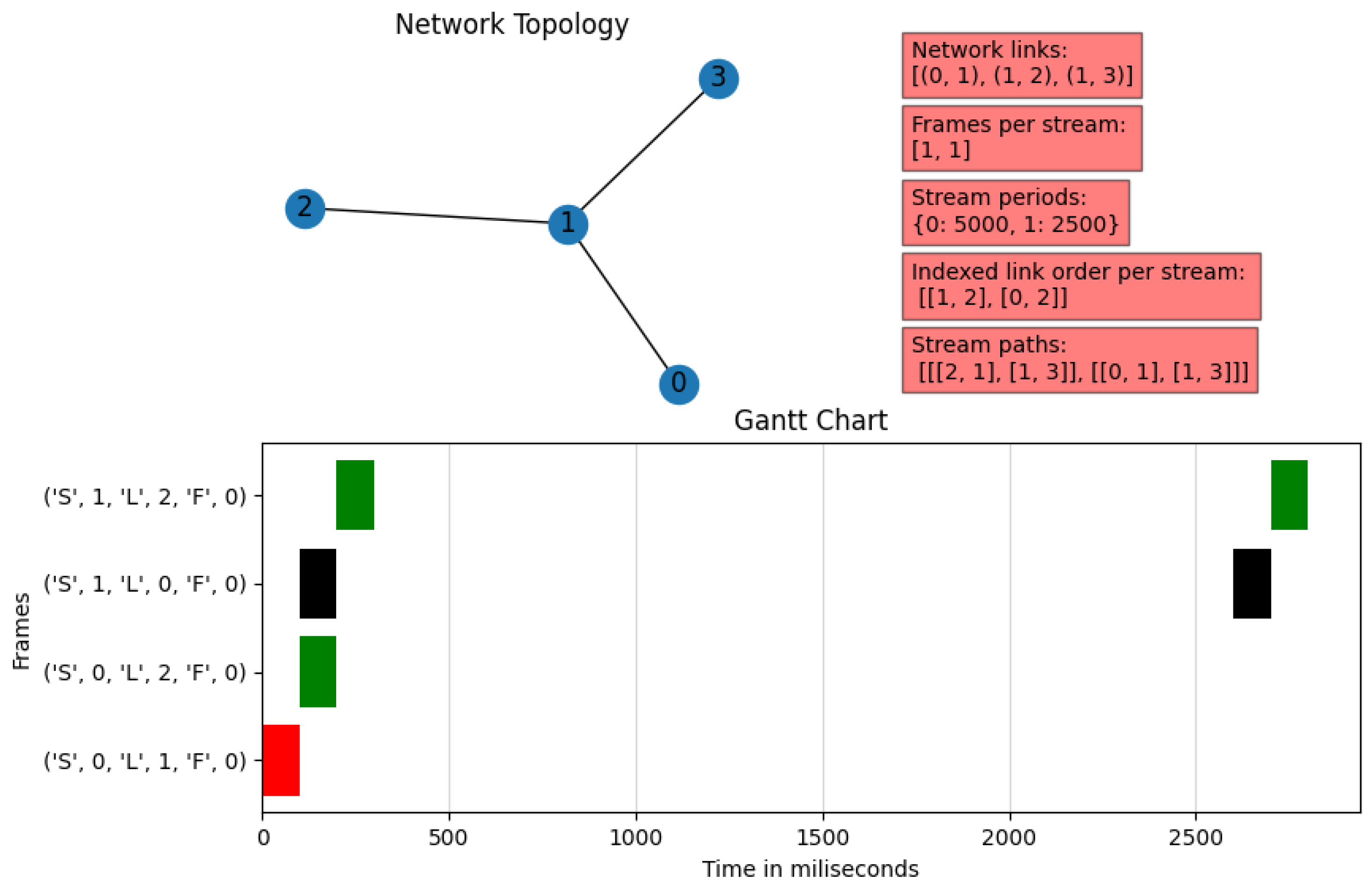
This subsection aims to verify that the results obtained by the combination between the Dijkstra algorithm output and the ILP scheduling are correct. As we have specified in the previous section, the main objective of the $\mu$TSN-CP is to be able to perform all the necessary calculations to find a specific and viable solution for a set of flows, taking into consideration that each stream will have an origin and destination, as well as its own characteristics in terms of bandwidth and maximum latency. We implemented a scheduling Solution Visualizer included in the ILP microservice to verify this goal, which includes the following (see Figure 9 as an example):

• Network topology: Specifies the network nodes and the links between them. It is located in the upper-left corner of the viewer.
• Description of the stream matrix: It includes a set of parameters such as the matrix of network links, the number of frames in each stream, the period of the flows, and an specification of the order of the links to be used according to the Dijkstra algorithm for each stream. These are written in two-dimensional vectors and dictionaries; the order in the array is the stream identifier. The parameters are in the upper-right corner of the diagram in red rectangles.
• Gantt diagram: This shows the used transmission slots, representing each link with a specific color; the horizontal axis depicts the time in milliseconds, while the vertical axis represents the position of the frames of each stream in each link. The notation employed on the vertical axis is as follows: ‘S’ is the frame stream number, ‘L’ is the link number through which the frame is traversing, and ‘F’ is the frame order within the stream. This graph is located at the bottom of the viewer.

We now describe three examples of the output provided by the visualizer after finding a solution to the scheduling problem. These examples were tested theoretically and using an auxiliary microservice that generates networking and TSN scheduling problems randomly.

4.1.1. Example 1

In this example, we present the features of the scheduling problem included in Figure 9:

• Four-node network, where Node 1 connects all other nodes.
• Two streams, each one with a single frame. Stream 0 has a period of 5000 ms, while Stream 1 has a period of 2500 ms.
• The fifth red box at the top right of the diagram contains an array of arrays that describes the paths from source to destination obtained using Dijkstra’s algorithm. In this example, Stream 0 traverses from Node 2 to Node 3, passing through Node 1, while Stream 1 traverses from Node 0 to Node 3, also passing through Node 1.

In the Gantt chart at the bottom of Figure 9, we can see that this solution fulfills all of the conditions of a TSN schedule, since there is no overlap between frames in both the same time slot and the same link; this is clear since no frame shares the same time interval with another frame of the same color. In addition, the example fulfills the usual assumption of any transmission: the streams pass through the links in sequential order. In the case of Stream 1, which has half the period of Stream 0, there exist repetitions in the hyper-period after 2500 ms.

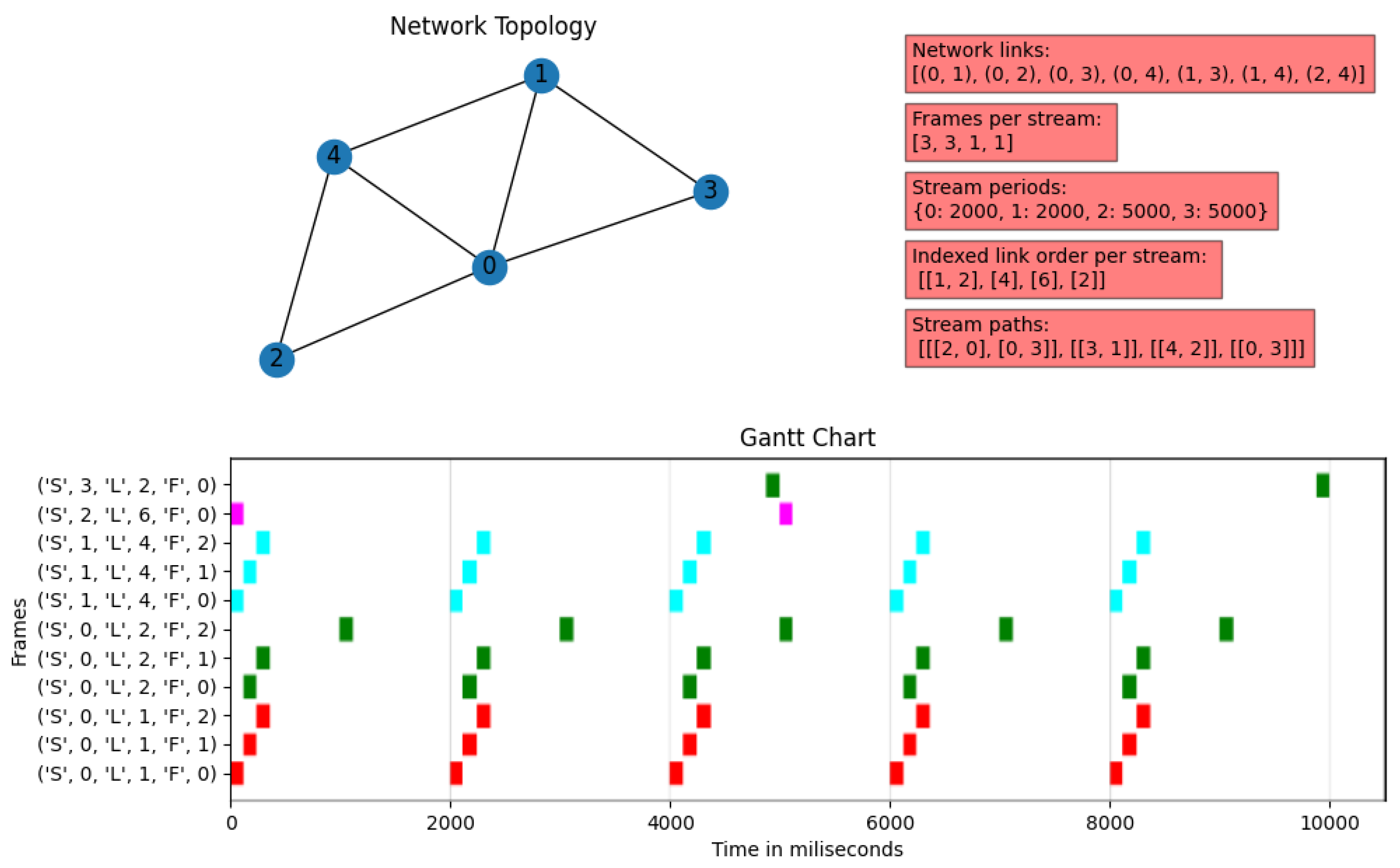
4.1.2. Example 2

The features of the second example are shown in Figure 10:

• Five-node network, where Node 2 connects all other nodes. Furthermore, Nodes 3 and 4 have a direct link between them.
• Four streams: Stream 0 consists of three frames, while the others have only one frame. The first stream has a period of 2000 ms, while the other streams have periods of 5000 ms, which makes the hyper-period 10,000 ms.
• The stream distribution is as follows:

  –

  Stream 0: origin at Node 3 and destination at Node 0, passing through Node 2.

  –

  Stream 1: origin at Node 0 and destination at Node 2.

  –

  Stream 2: origin at Node 3 and destination at Node 1, passing through Node 2.

  –

  Stream 3: origin at Node 2 and destination at Node 4.

This example is noticeably more complicated than the previous one. It involves a larger number of frames, a larger network, and more conditions to fulfill for the ILP due to the multiplicity of frames of some streams within the hyper-period. However, when looking at the image, we can appreciate that there is no overlapping of streams in any of the links simultaneously, even considering the repetitions in the hyper-period. In addition, the solver foresees when the successive frames of a stream will require an additional transmission time slot in a link, so it will prevent collisions between streams with multiple frames.

It is interesting to note that Stream 0 never interrupts Stream 1, even though they both use Link 0. However, the most crucial moment occurs with Streams 0 and 2 on Link 2. Although the frames of Stream 0 could have been transmitted consecutively on Link 2, this option would interfere when Stream 2 transmits over that link. Therefore, the system decides to leave a time slot free for Stream 2 to use, even if this is necessary only in the third repetition period.

4.1.3. Example 3

The constraints that describe this last example are listed below, and are depicted in Figure 11:

• Five-node network, where Node 0 connects the other nodes, but several nodes have direct connections to each other.
• Four streams, two of them made up of three frames; the other two have only one frame. The first two streams have periods of 2000 ms, while the other two have periods of 5000 ms, making the hyper-period 10,000 ms, as in the previous example.
• The stream distribution is as follows:

  –

  Stream 0: Origin at Node 2 and destination at Node 3, passing through Node 0.

  –

  Stream 1: origin at Node 3 and destination at Node 1.

  –

  Stream 2: origin at Node 4 and destination at Node 2.

  –

  Stream 3: origin at Node 0 and destination at Node 3.

In this example, we have increased the number of frames and used a topology with a higher number of links to explore whether the solutions delivered by our solver meet the constraints for a TSN scheduling system. We can notice that in none of the links, at any time, the location of one frame overlaps with another, even considering the repetitions that the frames may have within the hyper-period.

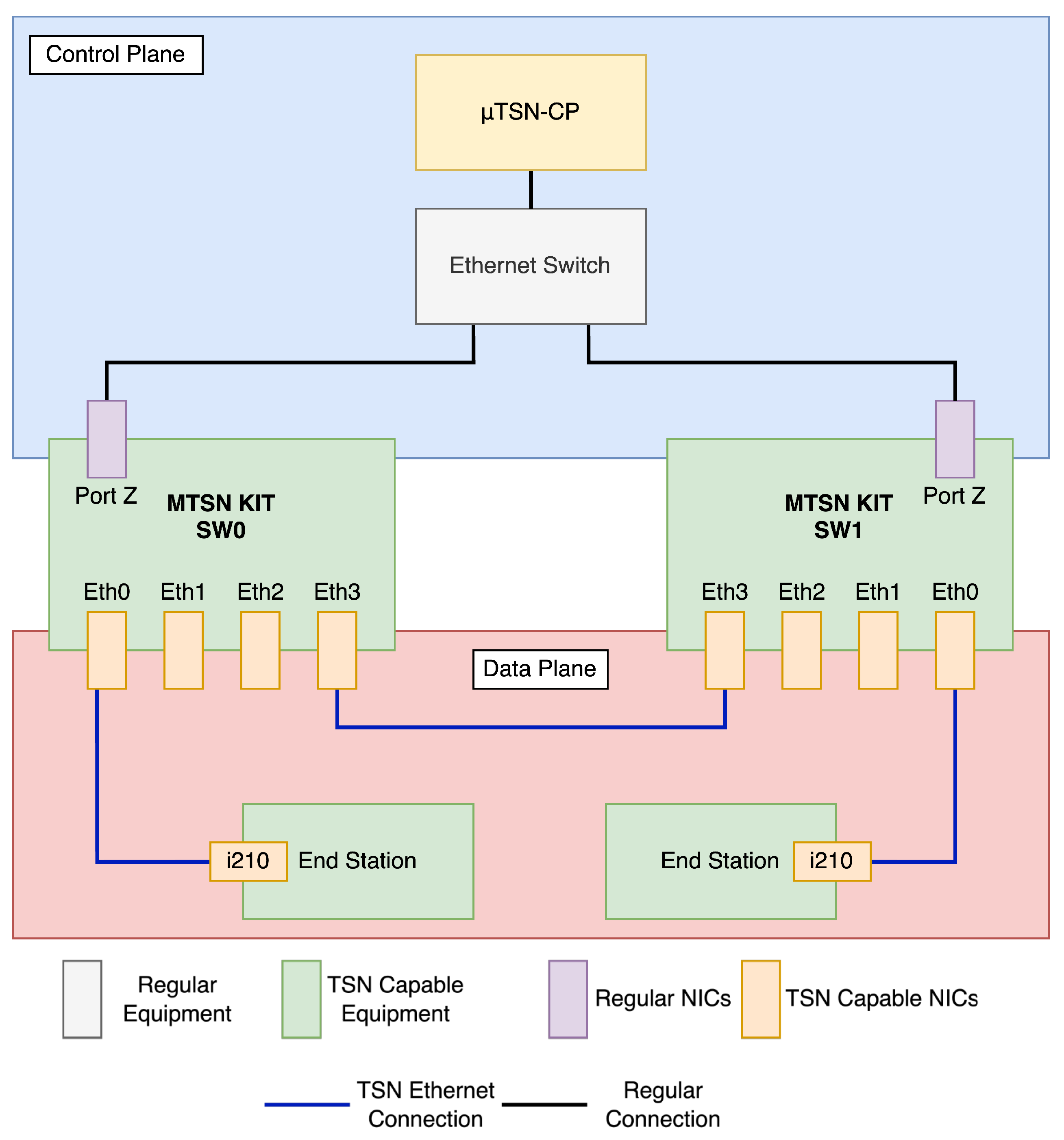
4.2. Laboratory Setup

The elements included in the setup are shown in Figure 12. We will start by distinguishing between the data plane and the control plane. The data plane consists of all the components within the red block. These elements have hardware interfaces that are capable of communicating according to TSN standards:

• Two TSN switches (SW0, SW1). We used Soc-e MTSN kits during the development and testing phase [31]. Each switch has four TSN interfaces; it communicates with the other switch through the Eth3 interface and with its respective end station through the Eth0 interface. PTP messages are exchanged in the TSN links for synchronization purposes.
• Two end stations. In our testbed, we used two computers running Linux (Ubuntu 22.01 LTS). Intel i210 network interface cards were used to support the precise timestamping required by PTP. The computers ran PTP daemons to manage synchronization with the switches.

On the other hand, the elements inside the blue block correspond to the control plane:

• The Port Z interfaces of the TSN switches. These NICs were used only for management tasks by means of NETCONF and SSH.
• A regular Ethernet switch that works as an out-of-band control network.
• The $\mu$TSN-CP Controller, deployed on a single computer with Docker-compose. This highlights another advantage of using microservices, as our controller can run on any machine with Docker. However, to take full advantage of the microservices architecture in a more realistic deployment, the $\mu$TSN-CP Controller should ideally be in a private or public cloud, running on some container orchestration tool like Kubernetes, OpenShift, or Docker Swarm.

4.3. Performance Analysis

We now describe performance tests to evaluate the resource usage of our design. First, it is important to note that, at the system’s core, there is a microservice with an ILP model that incorporates the constraints and defines the objective function of the TSN scheduling problem. This microservice can use any ILP solver, including those shown in Table 1. We compared GLPK and Gurobi in terms of the time they took to offer a solution for a given number of streams in a defined topology. Secondly, it is important to consider another condition that can affect the performance of our system: this is the hardware of the machine in which the ILP Calculator microservice runs. We ran our tests over three different platforms:

• A laptop with a four-core Intel Core i7-7820HK processor with a maximum frequency of 3.9 GHz and 16 GiB of RAM.
• An Elastic Compute Cloud (EC2) instance on Amazon Web Services (AWSs) of type T3.small with a two-core Intel Xeon Scalable processor with a maximum frequency of 3.1 GHz and 2 GiB of RAM [32].
• An EC2 instance on AWSs of type M5Zn.large with a four-core Intel Xeon Scalable processor with a maximum frequency of 4.5 GHz and 16 GiB of RAM [33].

According to the literature, the actual performance one will get from using multiple cores in an ILP problem depends on several factors, such as the nature of the optimization problem, the size of the model, the availability of memory resources, and the specific system configurations [34]. In this test we determined which is the option that provides a solution to the problem in the shortest time. Finally, with the results of the three previous experiments, we selected the best ILP model solver and compared the two platforms with the best performance to identify what characteristics the platform running the microservice should have, both in terms of hardware resources and solver.

We now describe the characteristics of the experiments. The topology is shown in Figure 13, where all links are 1 Gbps. Regarding flows, a custom microservice created the inputs of the Jetconf microservice, generating specifications sent through the RabbitMQ queue. All streams had a deadline of 500 ms. The periods of the streams varied between 125 ms, 250 ms, and 500 ms with uniform probability. The streams could be composed of one to three frames with the same probability. The number of streams went from fifteen to twenty-five streams per problem, with jumps of five streams between each test. We repeated each test 100 times for each number of streams.

4.3.1. Comparison of ILP Solvers

Previous works show that Gurobi generally offers better resolution times and performance than GLPK, especially for large and complex problems [35]. Indeed, in agreement with the literature, Figure 14 shows that the performance of Gurobi is considerably superior to that of GLPK. In the figure, the colored bar is the average value, and the segment in each bar denotes the minimum and maximum values.

While the time to find a solution using GLPK increases considerably, reaching up to 27 s maximum and 4.76 s on average in the first test with 15 streams, and up to a maximum of 80.63 s in the test with 25 streams, Gurobi times were never higher than 1.5 s, with average values of less than 1 s for all tests. An aspect that greatly differentiates the two solvers is the variance.

Table 2. Seconds needed to find a solution for GLPK vs. Gurobi, depending on the number of streams.

	GLPK				Gurobi
Streams	Average	Min	Max	Std. Dev.	Average	Min	Max	Std. Dev.
15	4.768	1.895	27.772	5.621	0.620	0.542	1.410	0.182
20	23.113	10.431	55.086	12.329	0.758	0.700	0.926	0.047
25	58.503	30.810	80.636	13.622	0.978	0.909	1.439	0.111

depicts the average time to solution value and the maximum and minimum values, together with the standard deviation. Considering this last value, Gurobi not only offers a higher performance, but also a much greater consistency than GLPK for our ILP model.

4.3.2. Hardware Configurations Comparison—Using GLPK

In this case, we used GLPK as an ILP solver to determine how much the hardware affects timing to obtain a solution to the scheduling problem. We considered RAM size, the number of processor cores, and the operating frequency. In Figure 15, each graph refers to a different number of streams; it should be noted that each graph has a vertical axis that covers different ranges. The figure shows that the best results were obtained using the M5Zn.large instance, although the difference with the local machine is not too large. The worst results were those obtained with the T3.small instance, which presents much greater solution times than the other two platforms. The T3.small instance has completely different hardware characteristics than the other two: it has much less RAM, fewer processor cores, and, perhaps the most important feature, its processor frequency is much lower than the other two platforms. On the other hand, the local machine and the M5Zn.large instance only differ in their clock frequency, since they have the same number of cores and the same RAM.

This test indicates that the hardware characteristics significantly affect the time to obtain a result.

Table 3. Seconds to find a solution with 15 streams: local machine vs. T3.small vs. M5Zn.large using GLPK.

Instance	Average	Min	Max	Std. Dev.
Local machine	3.125	1.895	4.560	0.798
AWSs T3 Small	4.263	2.584	9.051	1.484
AWSs M5Zn Large	3.503	1.287	9.672	2.426

,

Table 4. Seconds to find a solution with 20 streams: local machine vs. T3.small vs. M5Zn.large using GLPK.

Instance	Average	Min	Max	Std. Dev.
Local machine	19.154	10.431	55.086	11.244
AWSs T3 Small	129.062	13.994	267.103	75.260
AWSs M5Zn Large	18.370	7.488	48.252	11.461

and

Table 5. Seconds to find a solution with 30 streams: local machine vs. T3. small vs. M5Zn.large using GLPK.

Instance	Average	Min	Max	Std. Dev.
Local machine	255.013	30.810	1013.215	302.593
AWSs T3 Small	501.388	45.194	1546.723	478.889
AWSs M5Zn Large	162.642	12.672	634.854	135.549

show the average, maximum, and minimum values for each test as well as the standard deviation. In all cases, the results present considerable variations attributable to the lower consistency of GLPK. Actually, in the next test, where we only use Gurobi as an ILP solver, we observed a better consistency.

4.3.3. Hardware Configurations Comparison—Using Gurobi

In this test we used the two instances that showed the best performance in the previous test, namely the local machine and the M5Zn.large instance on AWSs. We used Gurobi as the ILP solver to obtain the best possible performance. According to AWSs, M5zn instances deliver the highest all-core turbo CPU performance from Intel Xeon Scalable processors in the cloud. Therefore, they are specifically designed to use the highest frequency possible in their processors.

Using Gurobi, the time needed to find solutions is considerably short when compared to using GLPK; for that reason, to differentiate both platforms better, we increased the number of streams in the same planning problem for all the tests. Therefore, the considered problems have 40, 45, and 50 streams. As Figure 16 reveals, the M5Zn.large instance performs much better than the local machine for all tests. We note that the difference between the maximum and the minimum values, as well as the stardard deviation, is considerably larger in the local instance. That fact indicates that the consistency of the performance with the M5Zn.large instance is greater.

Table 6. Seconds to find a solution: local machine vs. M5Zn.large using Gurobi, depending on the number of streams.

	Local Machine				MZ5n Large
Streams	Average	Min	Max	Std. Dev.	Average	Min	Max	Std. Dev.
40	57.570	51.236	64.660	4.675	2.201	2.024	2.328	0.089
45	87.403	75.829	105.118	8.256	3.070	2.673	3.598	0.212
50	138.381	112.855	163.418	14.569	4.255	3.779	4.573	0.247

shows the average time to obtain a solution, the maximum and minimum values, and the standard deviation obtained in the 100 repetitions of the tests. These results suggest that the clock frequency of the CPU for our particular problem is a transcendental parameter when it comes to reducing the time to obtain a solution. All the tests indicate that using the Gurobi solver with the M5Zn.large instance is the best combination to obtain the smallest run times.

5. Microservices as Deployment Strategy: A Qualitative Analysis

We have seen in the experiments that the characteristics of the hardware have a dramatic impact on the run times of certain computationally intensive tasks—specifically, the time schedule calculation—and the conclusion is that the run times of the ILP are much smaller if we use a specially designed machine with a high frequency of operation. In contrast, other tasks, e.g., the topology collection, do not require such stringent hardware specifications. This highlights the advantage of assigning different software tasks to separate microservices, to better align the hardware resources to their requirements. This represents a clear advantage of using the microservice approach above a monolithic implementation.

In an ideal scenario, the ILP should run on a high-capacity hardware computer, with the maximum operating frequency for its processor and using an efficient solver like Gurobi. In contrast, the rest of the elements could run on general-purpose machines, using container orchestration tools such as Kubernetes or OpenShift. Both tools allow us to manage where and when the containers containing the microservices are deployed and store their configuration parameters. They also provide components to expose the microservices to the outside and mechanisms to select the nodes on which the microservices can be deployed. However, these two technologies have significant differences: Kubernetes is a widely adopted, highly scalable, open-source container orchestration platform, which provides robust tools for container cluster management, application deployment, and autoscaling; on the other hand, OpenShift is a Kubernetes-based application platform developed by Red Hat that offers an additional layer of added value by providing a more complete and enterprise-ready experience. OpenShift incorporates Kubernetes but adds additional features and functionalities, such as deployment automation, application lifecycle management, and a more intuitive and simplified approach to application deployment. In short, while OpenShift is focused on offering a complete and enterprise solution, Kubernetes is a more basic and flexible option.

From all the previous considerations, we concluded that the ideal scenario to deploy our $\mu$TSN-CP solution consisted of a Kubernetes cluster comprising two groups of nodes. The first group is made up of machines specifically designed to operate at high frequency (for example, the AWSs M5Zn.large machine group), intended for the ILP Calculator microservice, while the second group comprises general-purpose hardware and is used to run all the other microservices. Figure 17 illustrates this approach.

6. Conclusions and Future Work

In this work, we described the development of a functional prototype of a TSN CP following the SDN architecture, and tested it using real equipment. In addition, we explored the characteristics of a microservice architecture (MSA) and its advantages. This kind of architecture can achieve better results than an equivalent monolithic architecture because it is possible to allocate resources tailored to the specific needs of each microservice. With an MSA, we have a superior granularity in the assignation of resources; in contrast, in a monolithic architecture, we cannot specifically allocate resources to specific software tasks. To the best of our knowledge, the only other works that have described SDN control planes for TSN that follow the microservices architecture are OpenCUC [14] (which is not yet public) and OpenCNC [15,17].

We described quantitatively how the MSA can be used to achieve superior scalability, by assigning computational resources to specific microservices according to their requirements. More specifically, our results emphasize the need to prioritize the processor clock speed of the machines that are running the ILP solver we used. This is because solving a linear programming problem is a single-thread task. It does not matter how many available cores the processor has; it will only use a single thread. This is the main reason why, during our experiments, the M5Zn.large AWSs machine outperformed the local machine. In a real scenario, it is thus possible to specifically allocate that microservice to a working device with the highest clock speed to achieve better results, thanks to the modular character of the MSA.

In the case of creating a Kubernetes cluster, the nodes with higher clock speed must be properly labeled so that the Kubernetes scheduler can assign the ILP pod to the optimal node. By strategically tagging nodes within a Kubernetes cluster that possesses superior computational capabilities, we can leverage the TaintToleration attribute of deployment resources in Kubernetes to precisely assign pods of a microservice to designated machines. This approach is particularly beneficial, for example, in the case of the ILP microservice, where we can apply a Taint to ensure that the ILP’s pods are exclusively scheduled on machines boasting higher CPU frequencies. This method enhances the efficiency and performance of resource-intensive applications by optimizing hardware utilization.

We are currently exploring several extensions to our work. To begin, the modular design provided by the MSA allows for better upgrading possibilities: we can replace individual components as long as the new microservice receives the same inputs and delivers the same outputs as the old one. This presents the additional advantage of being able to follow development and integration processes for different microservices separately. In this context, we are exploring the substitution of the current ILP Calculator microservice. ILP algorithms have exponential run times [2], so there is no guarantee that they will find a valid schedule before an established time. In practice, a deadline is set for the ILP algorithm to find a valid solution and, if it is not found, the schedule is considered to be unfeasible. Every execution of the ILP that results in an unfeasible outcome is thus a waste of computing effort and time. There exist other solutions to the scheduling problem in TSN that resort to Machine Learning (ML) in the literature, e.g., [36], but they do not contemplate the TAS defined in IEEE802.11Qbv. To the best of our knowledge, there exists no other work in the literature that proposes the use of ML to support the calculation of valid schedules for the TAS in TSN. In our ongoing work, we are using supervised ML to quickly predict the feasibility of a schedule and, only if the prediction is positive, go ahead with the execution of the ILP algorithm.

Following a microservices architecture also raises some security issues that must be addressed. In order to keep data safe, mutual TLS (mTLS) could be used for identification and encryption in the internal interactions between microservices. Regarding external (user) interaction with $\mu$TSN-CP, the entry point, which is the Jetconf microservice, already includes the option to transmit the stream list by means of HTTPS. Furthermore, adding a monitoring microservice could be useful to provide centralized log management.

Finally, $\mu$TSN-CP can be employed in integrated 5G-TSN scenarios such as those described in [37,38] for industrial communications, where a whole 5G network (typically private) acts as a single TSN switch. The $\mu$TSN-CP would communicate with the 5G system through an application function (AF) in order to coordinate the creation and transport of Quality-of-Service flows, considering the requirements of the TSN streams. Because of the flexibility of its architecture, it would not be difficult to add new microservices to $\mu$TSN-CP in order to interact with the 5G control plane.

References

- Gerhard, T.; Kobzan, T.; Blöcher, I.; Hendel, M. Software-defined flow reservation: Configuring IEEE 802.1 Q time-sensitive networks by the use of software-defined networking. In Proceedings of the 2019 24th IEEE International Conference on Emerging Technologies and Factory Automation (ETFA), Zaragoza, Spain, 10–13 September 2019; IEEE: New York, NY, USA, 2019; pp. 216–223. [Google Scholar] [CrossRef]
- Raagaard, M.L.; Pop, P. Optimization Algorithms for the Scheduling of IEEE 802.1 Time-Sensitive Networking (TSN); Technical Report, DTU Compute; Technical University of Denmark: Kongens Lyngby, Denmark, 2017; Available online: https://www2.compute.dtu.dk/~paupo/publications/Raagaard2017aa-Optimization%20algorithms%20for%20th-.pdf (accessed on 15 February 2024).
- IEEE. Standard for Local and Metropolitan Area Networks–Timing and Synchronization for Time-Sensitive Applications. In IEEE Std 802.1AS-2020 (Revision of IEEE Std 802.1AS-2011); IEEE: New York, NY, USA, 2020. [Google Scholar] [CrossRef]
- Quan, W.; Fu, W.; Yan, J.; Sun, Z. OpenTSN: An open-source project for time-sensitive networking system development. CCF Trans. Netw. 2020, 3, 51–65. [Google Scholar] [CrossRef]
- Kobzan, T.; Blöcher, I.; Hendel, M.; Althoff, S.; Gerhard, A.; Schriegel, S.; Jasperneite, J. Configuration Solution for TSN-based Industrial Networks utilizing SDN and OPC UA. In Proceedings of the 2020 25th IEEE International Conference on Emerging Technologies and Factory Automation (ETFA), Vienna, Austria, 8–11 September 2020; IEEE: New York, NY, USA, 2020; Volume 1, pp. 1629–1636. [Google Scholar] [CrossRef]
- Thi, M.T.; Said, S.B.H.; Boc, M. SDN-based management solution for time synchronization in TSN networks. In Proceedings of the 2020 25th IEEE International Conference on Emerging Technologies and Factory Automation (ETFA), Vienna, Austria, 8–11 September 2020; IEEE: New York, NY, USA, 2020; Volume 1, pp. 361–368. [Google Scholar] [CrossRef]
- Gallipeau, D.; Kudrle, S. Microservices: Building blocks to new workflows and virtualization. SMPTE Motion Imaging J. 2018, 127, 21–31. [Google Scholar] [CrossRef]
- Moradi, F.; Flinta, C.; Johnsson, A.; Meirosu, C. Conmon: An automated container based network performance monitoring system. In Proceedings of the 2017 IFIP/IEEE Symposium on Integrated Network and Service Management (IM), Lisbon, Portugal, 8–12 May2017; IEEE: New York, NY, USA, 2017; pp. 54–62. [Google Scholar] [CrossRef]
- Manso, C.; Vilalta, R.; Casellas, R.; Martínez, R.; Muñoz, R. Cloud-native SDN controller based on micro-services for transport networks. In Proceedings of the 2020 6th IEEE Conference on Network Softwarization (NetSoft), Ghent, Belgium, 29 June–3 July 2020; IEEE: New York, NY, USA, 2020; pp. 365–367. [Google Scholar] [CrossRef]
- Van, Q.P.; Tran-Quang, H.; Verchere, D.; Layec, P.; Thieu, H.T.; Zeghlache, D. Demonstration of container-based microservices SDN control platform for open optical networks. In Proceedings of the 2019 Optical Fiber Communications Conference and Exhibition (OFC), San Diego, CA, USA, 3–7 March 2019; IEEE: New York, NY, USA, 2019; pp. 1–3. [Google Scholar] [CrossRef]
- Orozco, G. A microservices-Based Control Plane for Time Sensitive Networking. Master’s Thesis, Universitat Politècnica de Catalunya, Barcelona, Spain, 2023. Available online: https://upcommons.upc.edu/handle/2117/392939 (accessed on 15 February 2024).
- Bierman, A.; Björklund, M.; Watsen, K. RESTCONF Protocol. RFC 8040. 2017. Available online: https://www.rfc-editor.org/info/rfc8040 (accessed on 15 February 2024).
- Enns, R.; Björklund, M.; Bierman, A.; Schönwälder, J. Network Configuration Protocol (NETCONF). RFC 6241. 2011. Available online: https://www.rfc-editor.org/info/rfc6241 (accessed on 15 February 2024).
- OpenCUC. 2020. Available online: https://github.com/openCUC/openCUC (accessed on 15 February 2024).
- OpenCNC Demo. 2022. Available online: https://git.cs.kau.se/hamzchah/opencnc_demo (accessed on 15 February 2024).
- OpenCNC: TSNService. Available online: https://git.cs.kau.se/hamzchah/opencnc_tsn-service (accessed on 15 February 2024).
- Hallström, F. Automating End Station Configuration: An Agile Approach to Time-Sensitive Networking. Master’s Thesis, Karlstad University, Karlstad, Sweden, 2023. Available online: https://www.diva-portal.org/smash/get/diva2:1784534/FULLTEXT02.pdf (accessed on 15 February 2024).
- Jetconf. Available online: https://github.com/CZ-NIC/jetconf (accessed on 15 February 2024).
- IEEE. Standard for Local and Metropolitan Area Networks–Bridges and Bridged Networks—Amendment 31: Stream Reservation Protocol (SRP) Enhancements and Performance Improvements. In IEEE Std 802.1Qcc-2018 (Amendment to IEEE Std 802.1Q-2018 as amended by IEEE Std 802.1Qcp-2018); IEEE: New York, NY, USA, 2022. [Google Scholar] [CrossRef]
- Congdon, P. Link Layer Discovery Protocol and MIB; Technical Report; IEEE: New York, NY, USA, 2002; Available online: https://www.ieee802.org/1/files/public/docs2002/lldp-protocol-00.pdf (accessed on 15 February 2024).
- Zadka, M. Paramiko. In DevOps in Python: Infrastructure as Python; Apress: Berkeley, CA, USA, 2019; pp. 111–119. [Google Scholar] [CrossRef]
- Integer Linear Programming. Available online: https://en.wikipedia.org/wiki/Integer_programming (accessed on 15 February 2024).
- Pyomo. 2008. Available online: https://github.com/Pyomo/pyomo (accessed on 15 February 2024).
- AMPL. 2022. Available online: https://ampl.com/ (accessed on 15 February 2024).
- Pico. 2022. Available online: https://www.swmath.org/software/2252 (accessed on 15 February 2024).
- CBC. 2022. Available online: https://www.coin-or.org/Cbc/ (accessed on 15 February 2024).
- GLPK. 2022. Available online: https://www.gnu.org/software/glpk/ (accessed on 15 February 2024).
- Gurobi. 2008. Available online: https://www.gurobi.com/ (accessed on 15 February 2024).
- IEEE 802.1Q Bridge Yang Model. Available online: https://github.com/YangModels/yang/blob/main/standard/ieee/published/802.1/ieee802-dot1q-bridge.yang (accessed on 2 July 2023).
- OpenDaylight. Available online: https://opendaylight.org/ (accessed on 2 July 2023).
- SOC-e. MTSN-Kit: A Comprehensive Multiport TSN Setup. Available online: https://soc-e.com/mtsn-kit-a-comprehensive-multiport-tsn-setup/ (accessed on 15 February 2024).
- T3 AWS Instances. Available online: https://aws.amazon.com/es/ec2/instance-types/t3/ (accessed on 15 February 2024).
- M5 AWS Instances. Available online: https://aws.amazon.com/es/ec2/instance-types/m5/ (accessed on 15 February 2024).
- Chakrabarty, K. Test scheduling for core-based systems using mixed-integer linear programming. IEEE Trans. Comput.-Aided Des. Integr. Circuits Syst. 2000, 19, 1163–1174. [Google Scholar] [CrossRef]
- Meindl, B.; Templ, M. Analysis of commercial and free and open source solvers for linear optimization problems. In Technical Report; Vienna University of Technology: Vienna, Austria, 2012; Available online: http://hdl.handle.net/20.500.12708/37465 (accessed on 15 February 2024).
- Mai, T.L.; Navet, N.; Migge, J. A Hybrid Machine Learning and Schedulability Analysis Method for the Verification of TSN Networks. In Proceedings of the 2019 15th IEEE International Workshop on Factory Communication Systems (WFCS), Sundsvall, Sweden, 27–29 May 2019; pp. 1–8. [Google Scholar] [CrossRef]
- 5GACIA. Integration of 5G with Time-Sensitive Networking for Industrial Communications. Technical Report, 5GACIA. 2021. Available online: https://archive.5g-acia.org/publications/integration-of-5g-with-time-sensitive-networking-for-industrial-communications/ (accessed on 15 February 2024).
- Ferré, M. Design and Development of a Gateway between Time-Sensitive Networking (TSN) and 5G Networks. Bachelor’s Thesis, Universitat Politècnica de Catalunya, Barcelona, Spain, 2023. Available online: https://upcommons.upc.edu/handle/2117/392883 (accessed on 15 February 2024).
Figure 1.
Overview of the TSN-CP prototype.
Figure 2.
Microservices architecture of the CP functions.
Figure 3.
Overview of the Jetconf microservice.
Figure 4.
Overview of the Topology Discovery microservice.
Figure 5.
Overview of the Preprocessing microservice.
Figure 6.
Overview of the ILP Calculator microservice.
Figure 7.
Overview of the Southconf microservice.
Figure 8.
Overview of the SDN Controller microservice.
Figure 9.
First scheduler problem.
Figure 10.
Second scheduler problem.
Figure 11.
Third scheduler problem.