A Scalable Approach to Minimize Charging Costs for Electric Bus Fleets

Abstract

Incorporating battery electric buses into bus fleets faces three primary challenges: a BEB’s extended refuel time, the cost of charging, both by the consumer and the power provider, and large compute demands for planning methods. When BEBs charge, the additional demands on the grid may exceed hardware limitations, so power providers divide a consumer’s energy needs into separate meters even though doing so is expensive for both power providers and consumers. Prior work has developed a number of strategies for computing charge schedules for bus fleets; however, prior work has not worked to reduce costs by aggregating meters. Additionally, because many works use mixed integer linear programs, their compute needs make planning for commercial-sized bus fleets intractable. This work presents a multi-program approach to computing charge plans for electric bus fleets. The proposed method solves a series of subproblems where the solution to the charge problem becomes more refined with each problem, moving closer to the optimal schedule. The results demonstrate how runtimes are reduced by using intermediate subproblems to refine the bus charge solution so that the proposed method can be applied to large bus fleets of 100+ buses. Not only will we demonstrate that runtimes scale linearly with the number of buses but we will also show how the proposed method scales to large bus fleets of over 100 buses while managing the monthly cost of energy.

1. Introduction

Battery electric buses (BEBs) are replacing diesel and natural gas buses in public transportation because they offer many benefits [1], including reduced maintenance [2], zero emissions [3], and access to renewable energy [4]. The challenge of prolonged charging times has been addressed in prior research with distributed charging networks [5], bus availability, environmental impact [6], route scheduling [7], battery health [8], the cost of electricity [9], and the cost of charging infrastructure [10].

One way in which previous authors have proposed managing the charge time of electric buses is through dynamic charging, which uses additional infrastructure to charge the vehicle while the vehicle is in motion. To this end, both overhead and inductive chargers have been proposed [11,12].

Inductive charging makes use of specialized hardware that is manufactured as part of the road or installed beneath to charge electric vehicles as they pass overhead. The benefits of such technology lie in how they wirelessly charge vehicles while they are in motion and reduce the need to stop for lengthy charge sessions. Unfortunately, such infrastructure is expensive and difficult to add once the road has already been constructed, which increases the cost of installation unless completed at the time of construction.

Overhead charging reaps similar benefits in that the vehicles under charge need not stop but differ in execution. Where inductive chargers operate wirelessly and remain part of the road, overhead chargers are installed separately and rely on mechanical hardware for connecting the BEB to the charging infrastructure. While easier to install after the initial road construction, the mechanical components require additional maintenance and the apparatus/overhead infrastructure is not aesthetically pleasing.

In the absence of dynamic charging solutions, many prefer to use static chargers to manage their energy needs. Static charging requires each BEB to stop for a period of time and connect to a charger to charge its battery. Unfortunately, charging in this manner leads to lengthy charge times, which requires careful planning to both meet the energy needs for BEBs and comply with the temporal scheduling demands of public transportation.

High-power chargers offer an alternative to slow charge times, decreasing the charge times by using increased rates of charge. Unfortunately, fast charging also increases the demands on the underlying electrical infrastructure [13] and can make power networks unreliable [14]. Power providers must then apply expensive upgrades [15] to the infrastructure, which can make fast charging cost-prohibitive.

Therefore, using static chargers to meet the energy requirements of an electric bus fleet requires a great deal of forethought and planning to meet both the temporal and energy demands of each BEB while managing the impact on the underlying electrical infrastructure [16]. Such foresight is generally too complex for any one individual and must be derived from a planning algorithm.

Planning methods can generally be considered either a heuristic approach [17], which trades optimality in favor of speed, or an exact approach, which considers all solutions to guarantee optimality. The exact approaches are also diverse, including graph-based network flow approaches [18,19], reinforcement learning [20], or other formulations using mixed integer linear programs (MILP) [21,22]. Generally, each method minimizes cost by either decreasing the instantaneous power needs for the fleet or optimizing around time-of-use tariffs [23,24].

The aforementioned approaches are feasible for many applications and are supported by additional work that estimates route times and energy demands [25], although the current methods do not scale with the number of buses while bounding the optimality of their solution.

Scaling these methods to large bus fleets (>100 BEBs) and numerous chargers is a challenge due to the size of the optimization problem that must be solved. For small fleets (<50 BEBs) and less than 10 chargers, the optimization problems in [18,21,23] have over ${10}^5$ variables (including binary and integer variables) and over ${10}^5$ constraints. Scaling to larger fleets and more chargers stresses computational resources and requires lengthy solve times.

This paper continues the theme of prior work, which is to develop charging schedules for electric buses that minimize the monthly electricity bill (energy consumption plus power demand) while satisfying route constraints that demand buses be in specific locations at specific times. One novelty is that our formulation considers the aggregated effects of loading across multiple meters. While meter aggregation is not widespread today, distribution networks must be built to supply worst case loads to each metered circuit. Therefore, our approach begins to explore how optimization of loads across multiple meters can reduce the overall impact of BEB charging on the grid. In this work, meter aggregation is modeled through the inclusion of uncontrolled (i.e., non-BEB charging) loads. Specifically, we incorporate historical load data from an electric train (UTA TRAX) that visits a central intermodal hub transit site in Salt Lake City, Utah, which is also a charging stop for BEBs.

The main contribution of the present paper is addressing the matter of scale. Rather than posing a single large MILP that incorporates every aspect of the charging problem, we solve a series of small subproblems in which the solution to the charging problem becomes successively more refined and moves closer to the optimal schedule. Our results show that intermediate subproblems can be solved with a dramatic reduction in runtimes, allowing our method to be applied to significantly larger bus fleets.

2. Methodology

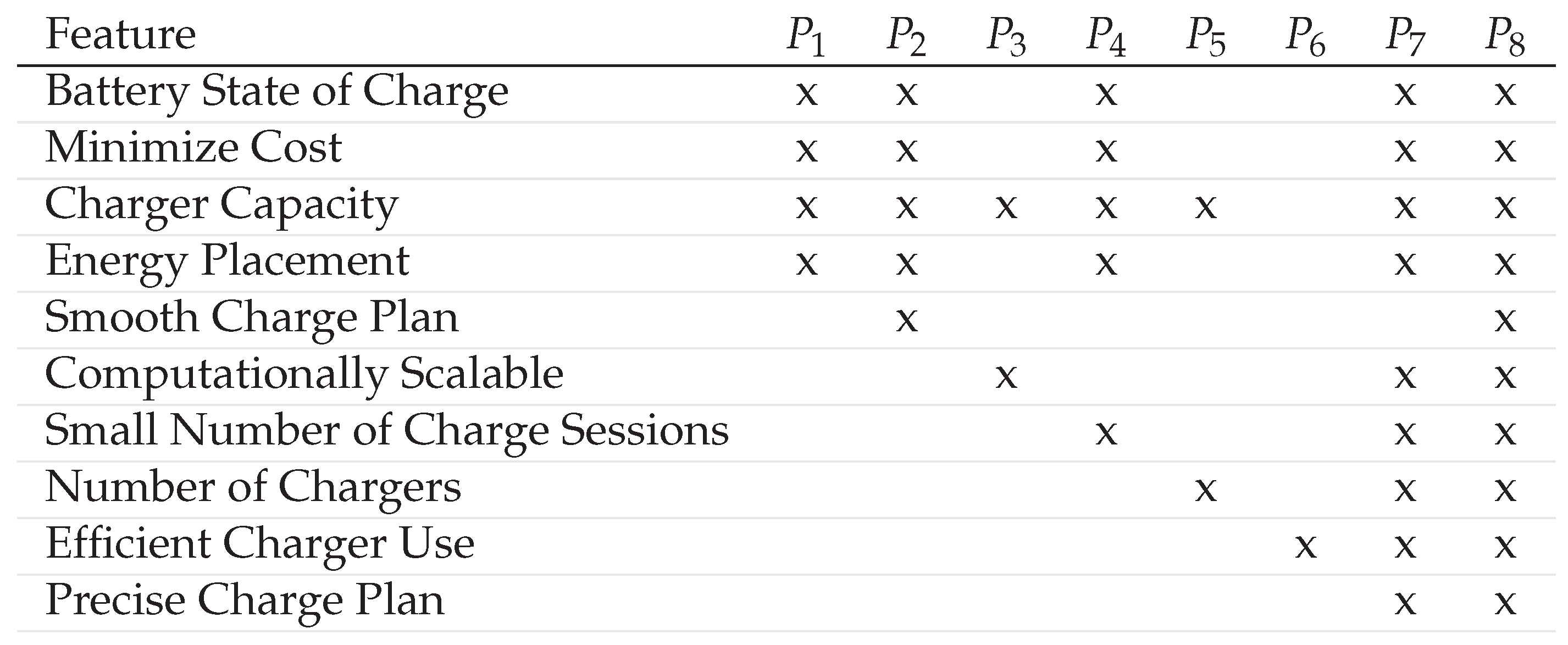
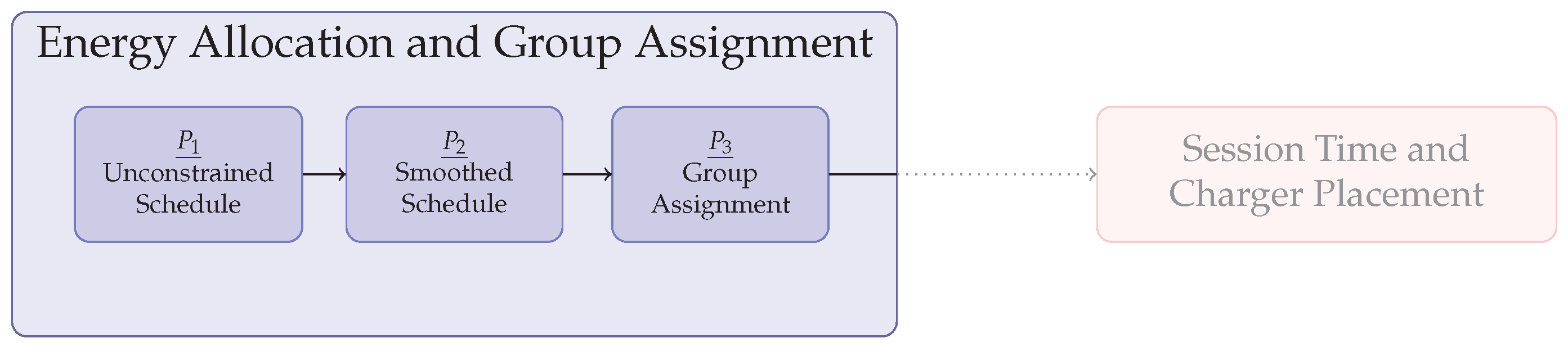
In a sense, this work explores what is gained in runtime by sacrificing some optimality in the schedule. The subproblems fall into three groups as shown in Figure 1. Each subproblem is solved using a linear, quadratic, or integer program, and, when used together, the series of programs provide a near optimal charge plan. Each subproblem addresses elements from one of three areas: energy allocation and bus grouping, session length and bus-to-charger assignments, and second-by-second optimization.

The energy allocation and bus grouping section has two objectives. The first determines a relaxed charge schedule that does not account for a limited number of chargers. The relaxed schedule provides information about ideal charge times for each bus that is refined in subsequent problems to account for the additional constraints. The second objective separates buses into groups where only buses in the same group may share chargers. Dividing buses into groups allows each group to be treated independently in future programs, which greatly simplifies the compute complexity of each subproblem.

The session-length and bus-to-charger assignment problems refine the relaxed solution provided in the first set of problems to account for a limited number of chargers and uses the unconstrained solution from the first part to compute a high-level charge schedule that includes a charger assignment, energy requirement, and start/end time for each bus’s charge session.

The second-by-second optimization section uses the schedule from the previous problems to compute a second-by-second plan of how energy will be delivered to each bus, resulting in a charge plan that includes when, at which charger, and how energy will be delivered to each bus to optimally manage the cost of energy. The table provided in Figure 2 lists each subproblem and which features each problem incorporates.

Note: A table with each variable in the paper is contained in Appendix A 

Table A1. Variables and definitions.

Variable	Description	Range	Variable	Description	Range
Indices
i	Bus index	$\mathbb{N}$	j	Time Index	$\mathbb{N}$
k	Charger index	$\mathbb{N}$	r	Route Index
m	group index	$\mathbb{N}$
Optimal Solution|Formulation
$n_{\mathrm{bus}}$	The number of buses in the optimization framework.	$\mathbb{Z}$	$n_{\mathrm{time}}$	The number of time indices in a day.	${\mathbb{Z}}^{+}$
$b_{p(i,j)}$	The average power consumed by bus i during time period j.	$\mathbb{R}$	$t_j$	The time at time index j. This paper also refers to the period of time from $t_j$ to $t_{j+1}$ as “period $t_j$”.	$\mathbb{R}$
$\mathit{b}$	A vector containing each value for $b_{p(i,j)}$.	${\mathbb{R}}^{n_{\mathrm{bus}}·n_{\mathrm{time}}}$	$\tilde{\mathcal{A}}$	The complement of $\mathcal{A}$.	$i\times j$
$\mathcal{A}$	The set of all $i\times j$ elements where bus i can charge at time index j	$i\times j$	$p_{\max }$	The maximum power a bus charger can deliver to a bus in kW. This paper assumes a value of 350 for most examples and results.	${\mathbb{R}}^{+}$
Optimal Solution|Battery
$h_{\min }$	The minimum allowable state of charge	$\left(0,h_{\max }\right)$	$h_{\max }$	The maximum state of charge	${\mathbb{R}}^{+}$
${\eta }_i$	The beginning state of charge for bus i	$\left(h_{\min },h_{\max }\right)$	$h\left(ij\right)$	The state of charge for bus i at time $t_j$.	$\left(h_{\min },h_{\max }\right)$
$\Delta T$	The change in time from $t_j$ to $t_{j+1}$	${\mathbb{R}}^{+}$	$\mathit{h}$	A vector containing all state of charge values.	${\mathbb{R}}_{+}^{n_{\mathrm{bus}}·n_{\mathrm{time}}}$
$\delta \left(ij\right)$	The battery discharge for bus i during time period j.	${\mathbb{R}}_{+}$	$h(i,\mathrm{end})$	Bus i’s final state of charge.	$\left(h_{\min },h_{\max }\right)$
Optimal Solution|Cumulative Load Management
$n_{\mathrm{charger}}$	The time index for the start of bus i’s jth stop	${\mathbb{Z}}_{+}$	$p_c\left(j\right)$	The average power consumed by all buses during time period j.	$\mathbb{R}$
${\mathit{p}}_{\mathit{c}}$	A vector containing all values of $p_c\left(j\right)$.	${\mathbb{R}}_{+}^{n_{\mathrm{time}}}$	$J_{\mathrm{thrash}}$	A secondary objective function that penalizes multiple plug-in instances per charge session.	${\mathbb{R}}_{+}$
$g(i,j)$	A slack variable used to compute the absolute value of $|b_{p(i,j)}-b_{p(i,j-1)}|$	${\mathbb{R}}_{+}$
Optimal Solution|Objective
${\mu }_{\text{e-on}}$	On-Peak Energy Rate	${\mathbb{R}}_{+}$	${\mu }_{\text{e-off}}$	Off-Peak Energy Rate	${\mathbb{R}}_{+}$
${\mu }_{\text{p-on}}$	On-Peak Demand Power Rate	${\mathbb{R}}_{+}$	${\mu }_{\text{p-all}}$	Facilities Power Rate	${\mathbb{R}}_{+}$
${\mathcal{S}}_{\mathrm{on}}$	The set of on-peak time indices	$\{1,\dots ,n_{\mathrm{time}}\}$	$p_{\mathrm{demand}}$	Maximum average power during on-peak periods	$\mathbb{R}$
$p_{\mathrm{facilities}}$	Maximum average power over all time instances.	${\mathbb{R}}_{+}$	$p_t\left(j\right)$	The total average power consumed by both the bus chargers and the uncontrolled loads.	${\mathbb{R}}_{+}^{n_{\mathrm{time}}}$
$u\left(j\right)$	The average power over time j consumed by the uncontrolled loads	${\mathbb{R}}_{+}^{n_{\mathrm{time}}}$	${\mathit{p}}_t$	a vector containing $p_t\left(i\right)$ for all i.	${\mathbb{R}}_{+}^{n_{\mathrm{time}}}$
$e_{\mathrm{on}}$	The total amount of energy consumed by the bus chargers and uncontrolled loads during off-peak hours.	${\mathbb{R}}_{+}$	$e_{\mathrm{off}}$	The total energy consumed by the bus chargers and uncontrolled loads during on-peak hours.	${\mathbb{R}}_{+}$
$J_{\mathrm{cost}}$	The section of the objective function pertaining to the fiscal expense of charging buses.	$\mathbb{R}$	$J_{\mathrm{all}}$	The expression for the complete objective function.	$\mathbb{R}$
Scalability
$n_{\mathrm{group}}$	The number of groups in which to divide the buses and available chargers in preparation for the $P_4$, $P_5$, and $P_6$.	${\mathbb{Z}}_{+}$	$n_{\mathrm{charger}}^m$	The number of chargers assigned to group m.	${\mathbb{Z}}_{+}$
$n_{\mathrm{bus}}^m$	The number of buses in group m.	${\mathbb{Z}}_{+}$	$p(j,m)$	The total power used during time index j by all buses in group m.	${\mathbb{R}}_{+}$
$\beta (i,m)$	A binary selector variable that is one when bus i is in group m and zero otherwise.	$\{0,1\}$	$n_{\mathrm{charger}}^m$	The number of chargers assigned to group m	${\mathbb{Z}}_{+}$
$\varphi (i,i^{\prime })$	The inner product of the optimal charge schedules for buses i and $i^{\prime }$, respectively.	${\mathbb{R}}_{+}$	$v(i,i^{\prime },g)$	A variable that is $w(i,i^{\prime })$ when buses i and $i^{\prime }$ are in group g and zero otherwise.	${\mathbb{Z}}_{+}$
$M_s$	The maximum value for $\varphi (i,i^{\prime })$.	${\mathbb{R}}_{+}$	$J_{\mathrm{select}}$	The objective function for the group selection problem	${\mathbb{R}}_{+}$
Defragmentation
$\theta (i,r)$	A binary variable that is one when charge session r from bus i will be used in a defragmented solution.	$\{0,1\}$	$\rho (i,r)$	A vector whose elements are equal to $\Delta T$ during time indices when bus i is charging during charge session r and zero otherwise.	${\mathbb{R}}^{n_{\mathrm{time}}}$
$\psi (i,j)$	The minimum allowable energy delivered to bus i during charge session r where the session in question is considered “active”.	$\mathbb{R}$	$\omega$	The minimum allowable energy for any charge session.	$\mathbb{R}$
$e_{\max }$	The maximum allowable energy delivered in any session.	$\mathbb{R}$
Charge Schedules
$a(i,r)$	The beginning of the allowable charge interval for bus i’s $r\mathrm{th}$ charge session.	${\mathbb{R}}_{+}$	$b(i,r)$	The commanded start time for bus i’s $r\mathrm{th}$ charge session	$\mathbb{N}$
$f(i,r)$	The commanded end time for bus i’s $r\mathrm{th}$ charge session.	${\mathbb{R}}_{+}$	$d(i,r)$	The end time of the allowable charge interval for bus i’s $r\mathrm{th}$ charge session.	${\mathbb{R}}_{+}$
$\sigma (i,r,k)$	A selector variable that is one when bus i charges at charger k for session r.	$\{0,1\}$	M	The number of seconds in a day	${\mathbb{Z}}_{+}$
$l(i,r,i^{\prime },r^{\prime })$	A selector variable that is one when bus i charges before bus $i^{\prime }$ during the r and $r^{\prime }$ sessions respectively.	$\{0,1\}$
Optimizing Charge Schedules
$c(s,i,r)$	The start time for bus i’s $r\mathrm{th}$ charge session.	$\mathbb{R}$	$c(f,i,r)$	The stop time for bus i’s $r\mathrm{th}$ charge session.	$\mathbb{R}$
$c(a,i,r)$	The arrival time of bus i for charge session r.	$\mathbb{R}$	$c(d,i,r)$	The departure time for bus i after having completed the $r\mathrm{th}$ charge session	$\mathbb{R}$
$J_{\mathrm{window}}$	The loss function that drives charge windows to the desired length.	$\mathbb{R}$
Multi-Rate Charging
$x(i,j)$	The final charge schedule for bus i at time j, yielding the power at which bus i will charge.	${\mathbb{R}}_{+}$	$z\left(j\right)$	The total power used by all buses at time j. ${\mathbb{R}}_{+}$
$\gamma (i,d)$	A binary vector that is one at all time steps where bus i charges during charge session d.	${\{0,1\}}^{n_{\mathrm{time}}}$	$e(i,r)$	The amount of energy to be delivered to bus i during charge session r.	${\mathbb{R}}_{+}$
$J_{\text{multi-rate}}$	The objective function over which we minimize to solve the multi-rate section of the bus charge problem.	$R_{+}$

.

2.1. Energy Allocation and Group Assignment

The first set of problems answers two primary questions: (1) at what time should energy be delivered to each bus, and (2) which buses are most able to share a charger. These questions are addressed through three subproblems: unconstrained charge schedule, smooth charge schedule, and group separation as shown in Figure 3.

The unconstrained schedule problem (denoted $P_1$), which is described in Section 2.1.1, computes an optimal charge schedule that minimizes the monthly cost of power in the presence of uncontrolled loads under the assumption that each bus has a dedicated charger.

The smooth schedule problem (denoted $P_2$), which is described in Section 2.1.2, has the same form as $P_1$ except for two differences. First, the monthly cost is required to match the optimal cost from the solution to the unconstrained scheduling problem $P_1$. Second, the objective for the smooth schedule problem $P_2$ penalizes change in the scheduled charge rates.

The group assignment problem (denoted $P_3$), which is described in Section 2.1.3, uses the charge schedules from $P_2$ to separate buses into groups such that the bus schedules within a group overlap as little as possible. Separating the scheduling problem into groups helps to manage the number of computations in succeeding optimization problems by reducing the size of these problems.

2.1.1. Unconstrained Schedule ($P_1$)

This section describes a program that finds a charge schedule where buses are allowed to charge without regard for the number of available chargers. This solution is considered “optimal” and will be used in later sections to formulate a feasible solution that accounts for the actual number of chargers available.

Formulation

The cost objective we minimize is based on the rate schedule from [26], which contains two primary elements: the cost of energy and power demand. Energy is billed per kWh using different rates for on-peak and off-peak hours. Demand is divided into two components. The first is a facilities charge, which is billed per kW for the highest 15 min average power use over the course of the month. The second is a demand charge, which is also billed per kW but is only billed for the highest 15 min average power used during on-peak hours. The rates for each component are provided in

Table 1. Description of the billing structure.

	On-Peak	Off-Peak	Facilities (Both)
Energy Rate	USD 0.058282/kWh	USD 0.029624/kWh	None
Energy Rate Symbol	${\mu }_{\text{e−on}}$	${\mu }_{\text{e−off}}$	None
Power Rate	USD 15.73/kW	None	USD 4.81/kW
Power Rate Symbol	${\mu }_{\text{p−on}}$	None	${\mu }_{\text{p−all}}$

.

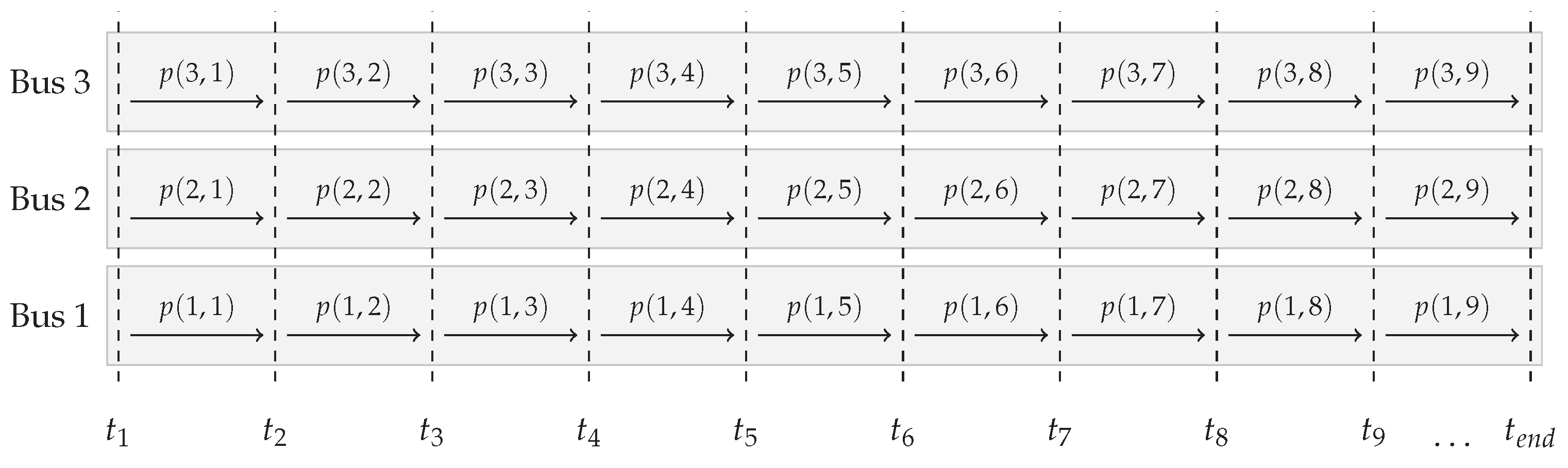
Before computing the total monthly cost of electricity, we must define expressions for average power and energy over time. Let each day be divided into time intervals of length $\Delta T$ where the average power consumed by bus i during time j is denoted $p(i,j)$ as shown in Figure 4. Note that $\Delta T$ may be chosen to be on the order of a second or minute, and expressions for 15 min averages will be derived later. The solution will yield the average power consumed by each bus during each time interval.

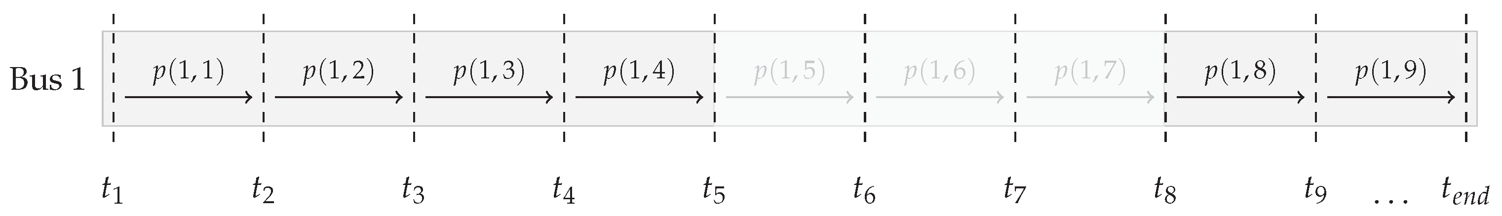
The time windows when each bus is available for charging must be accounted for as constraints. The maximum average power is set to zero when a bus is away from the station. For example, if bus 1 were out on route for times $t_5, t_6,$ and $t_7$, then the average power for those periods would be equal to zero as shown in Figure 5. Let $b_{p(i,j)}$ be the average power used by bus i at time index j, and $\mathit{b}$ be a vector that contains $b_{p(i,j)}$ for each bus and time index. Also, let $\mathcal{A}\subset i\times j$ be the set of all indices where bus i is in the station during time $t_j$ and let $\tilde{\mathcal{A}}$ be its complement. Also, let $p_{\max }$ be the maximum power that a charger can deliver.

The set of constraints that buses do not use power when not in the station are provided by

$$\begin{array}{c}{b}_{p(i,j)}=0\forall i,j\in \tilde{\mathcal{A}}\end{array}$$

(1)

$$\begin{array}{c}0\le b_{p(i,j)}\le p_{\max }\forall i,j\in \mathcal{A}\end{array}$$

(2)

Battery

Each bus must also maintain its state of charge above a minimum acceptable level throughout the day. When buses leave the station, their batteries discharge energy as they traverse their routes. Let $\delta (i,j)$ be the amount of charge lost by bus i at time j and let $h(i,j)$ be the state of charge of bus i at time j. The state of charge for each bus can be defined as

$$\begin{array}{cc}\hfill h(i,j)& =h(i,j-1)+b_p(i,j-1)·\Delta T-\delta (i,j)\forall i,j>1\hfill \\ \hfill h(i,1)& ={\eta }_i\forall i\hfill \end{array}$$

(3)

where ${\eta }_i$ is the initial state of charge for bus i and $\Delta T$ is the difference in time between $t_{i,j}$ and $t_{i,j+1}$. Now that each value for the state of charge is defined, each value for h must be constrained so that it is greater than a minimum acceptable value $h_{\min }$ but does not exceed the maximum battery capacity $h_{\max }$. This yields

$$\begin{array}{c}\hfill h_{\min }\le h(i,j)\le h_{\max }\forall i,j\end{array}$$

(4)

The final battery-related constraint has to do with how we are planning for the bus. The expenses that come from power are computed monthly, but we desire to simulate the movements of the bus for only a day and use this to extrapolate what the monthly cost may be. Therefore, the state of charge for a bus at the end of the day must reflect its starting value. This yields the following constraint:

$$h(i,\mathrm{end})=h(i,1)\forall i.$$

(5)

Cumulative Load Management

While this formulation does not directly account for the number of available chargers, we do account for the cumulative load capacities of all chargers. Let the number of chargers be denoted $n_{\mathrm{charger}}$. We desire to maintain the average cumulative power for each time step at a level that is serviceable given $n_{\mathrm{charger}}$. We define a slack variable $p_c\left(j\right)$, which represents the total average power consumed by all buses at time j. The variable $p_c\left(j\right)$ is computed as the sum of average bus powers so that

$$p_c\left(j\right)=\sum _i{b}_{p(i,j)}.$$

(6)

Objective

Now that the relevant constraints have been addressed, we turn attention to the objective function. We start by computing the total average power for the complete system. This total power is composed of power used by the buses and power used by external sources such as lights, ice melt, electric trains, etc., which we refer to as “uncontrolled loads”, where the average power for the uncontrolled loads at time step j is denoted $u\left(j\right)$. We compute the total power as the sum of power used by the buses $p_c\left(j\right)$ and the power consumed by uncontrolled loads $u\left(j\right)$ so that the total power, denoted $p_t\left(j\right)$, is computed as

$$p_t\left(j\right)=p_c\left(j\right)+u\left(j\right).$$

(7)

The next step is to compute the fifteen minute average power use for each time step, denoted $p_{15}$. We accomplish this by letting

$$p_{15}\left(j\right)=\frac{1}{n}\sum _{l\in \left\{j_{15}\right\}}{p}_t\left(l\right)$$

(8)

where $\left\{j_{15}\right\}$ is the set of all indices 15 min prior to time $t_j$ and n is the cardinality of $\left\{j_{15}\right\}$. Next, note that the rate schedule requires both the maximum overall average power, denoted $p_{\mathrm{facilities}}$, and the maximum average power during on-peak hours, or $p_{\mathrm{demand}}$. Let ${\mathcal{S}}_{\mathrm{on}}$ be the set of time indices belonging to on-peak hours, and recall that the max over all average power values is greater than or equal to $p_{15}\left(j\right)$ for all j. We can express this constraint as

$$p_{\mathrm{facilities}}\ge p_{15}\left(j\right)\forall j.$$

(9)

Because $p_{\mathrm{facilities}}$ makes up part of the objective function, the optimization algorithm will reduce the value for $p_{\mathrm{facilities}}$ until it is equal to the largest value in $p_{15}$. Following similar logic, we also define a set of constraints for the maximum average on-peak power $p_{\mathrm{demand}}$ so that

$$p_{15}\left(i\right)\le p_{\mathrm{demand}}\forall i\in {\mathcal{S}}_{\mathrm{on}}.$$

(10)

The next step in computing the objective function is to compute the total energy consumed during on- and off-peak hours, respectively. Let $e_{\mathrm{on}}$ be the total energy consumed during on-peak hours and $e_{\mathrm{off}}$ be the energy consumed during off-peak hours. We can compute energy as the product of average power and time. In our case, we compute this as

$$\begin{array}{cc}\hfill e_{\mathrm{on}}& =\Delta T·\sum _{i\in {\mathcal{S}}_{\mathrm{on}}}{p}_t\left(i\right)\hfill \\ \hfill e_{\mathrm{off}}& =\Delta T·\sum _{i\notin {\mathcal{S}}_{\mathrm{on}}}{p}_t\left(i\right).\hfill \end{array}$$

(11)

We can now compute the total monthly cost in dollars as

$$J_{\cos \mathrm{t}}={\left[\begin{array}{c}{e}_{\mathrm{on}}\\ e_{\mathrm{off}}\\ p_{\mathrm{facilities}}\\ p_{\mathrm{demand}}\end{array}\right]}^T\left[\begin{array}{c}{\mu }_{\text{e−on}}\\ {\mu }_{\text{e−off}}\\ {\mu }_{\text{p−all}}\\ {\mu }_{\text{p−on}}\end{array}\right]$$

(12)

The final optimization problem that computes a charge schedule without constraints on the number of chargers is described below.

We have observed that charge commands in solutions to $P_1$ tend to switch frequently between 0 and $p_{\max }$, which is difficult to implement in practice and imparts stress on charging hardware. Before additional steps can be taken, a smoother set of charge commands is computed, and this is the subject of the next section.

2.1.2. Unconstrained Smooth Schedule ($P_2$)

This section implements smoothing criteria so that the frequent “on-off” switching patterns from $P_1$ are reduced. This is completed by modifying $P_1$ in two ways. The first is that the demand, facilities, on-peak energy, and off-peak energy are removed from the objective and constrained to equal their values obtained in the solution to $P_1$ so that

$$\begin{array}{cc}\hfill e_{\mathrm{on}}& ={\tilde{e}}_{\mathrm{on}}\hfill \\ \hfill e_{\mathrm{off}}& ={\tilde{e}}_{\mathrm{off}}\hfill \\ \hfill p_{\mathrm{facilities}}& ={\tilde{p}}_{\mathrm{facilities}}\hfill \\ \hfill p_{\mathrm{demand}}& ={\tilde{p}}_{\mathrm{demand}},\hfill \end{array}$$

(13)

where values on the right-hand side are constants extracted from the solution to $P_1$. Next, we define an alternative objective that incentivizes continuity of charging between time steps. This objective is defined as

$$J_{\mathrm{switch}}=\frac{1}{n}\sum _{i,j,\in \mathcal{K}}{\parallel b(i,j)-b(i,j-1)\parallel }_2^2,$$

(14)

where $\mathcal{K}$ is the set of all $i,j$ where bus i may charge during time j and $j-1$. The final optimization problem that produces smooth charging schedules is provided below.

The solution to $P_2$ smooths charge schedules without increasing costs, but it presents the undesirable feature that the charge sessions tend to be fragmented into many short sessions. Additionally, the schedule does not account for the number of chargers or bus contention for charger use. Unfortunately, addressing these problems requires the use of binary variables, and optimization with binary variables becomes intractable for large numbers of buses and chargers. Before the fragmentation and charger assignment problems can be addressed, we first segment the buses into groups. Successive processing can be completed separately in groups, which helps to manage the computational complexity for later problems that incorporate binary variables.

2.1.3. Group Assignment ($P_3$)

This section addresses the matter of problem size. The complexity of the problem is strongly influenced by contention, which arises as multiple buses must share limited charging resources. The number of binary variables in the optimization problem increases as $n^2$, where n is the number of charge sessions. Before we can formulate a solution to the bus problem that scales linearly with n, we propose a method to separate buses into groups to reduce the coupling between charge sessions.

The group assignment problem separates buses into $n_{\mathrm{group}}$ groups, where group m is allocated $n_{\mathrm{charger}}^m$ chargers and $n_{\mathrm{bus}}^m$ buses. Each group must have sufficient chargers to fill its needs and prefer buses with dissimilar schedules to better avoid contention. We know that the number of cross-terms in future problems will be reduced when each group has the same number of buses. Therefore, let $n_{\mathrm{bus}}^m$ be described as

$$\begin{array}{cc}\hfill n_{\mathrm{bus}}^m& \ge ⌊\frac{n_{\mathrm{bus}}}{n_{\mathrm{group}}}⌋\hfill \\ \hfill n_{\mathrm{bus}}^m& \le ⌈\frac{n_{\mathrm{bus}}}{n_{\mathrm{group}}}⌉,\hfill \end{array}$$

(15)

where the values $n_{\mathrm{bus}}$ and $n_{\mathrm{group}}$ are user parameters.

The number of chargers assigned to each group must be exactly equal to the number of available chargers so that

$$n_{\mathrm{charger}}=\sum _m{n}_{\mathrm{charger}}^m.$$

(16)

The next set of constraints ensures that each bus is part of a group exactly once. Let $\beta (i,m)$ be a binary variable that is one when bus i is in group m. Each bus is constrained to be a member of exactly one group by letting

$$\sum _m\beta (i,m)=1\forall i.$$

(17)

We must also ensure that buses are assigned to groups where the power delivered to each bus can be achieved with the number of chargers assigned to that group. Define a slack variable that provides the total power used in group m at time step j as $p(m,j)$. Recall that we also know the expected power use for each bus as this is a result of $P_1$ as $b_{p(i,j)}$, which allows us to describe the total power for any one group as

$$p(m,j)=\sum _i\beta (i,m)b_{p(i,j)}.$$

(18)

Next, we know that the total load of each group must be less than or equal to the collective capability of that group’s chargers, which can be expressed as

$$n_{\mathrm{charger}}^m·p_{\max }\ge p(m,j)\forall m,j$$

(19)

so that the number of chargers is sufficient to charge the collective load of the group.

We also desire to group together buses whose routes have the least overlap. If two buses contain no overlap, they will be easiest to schedule on the same charger. The overlap is measured using the inner product of their schedules from $P_1$. If completely non-overlapping, the inner product will be equal to zero. Let

$$\varphi (i,i^{\prime })=\mathbf{b}{(i,:)}^T\mathbf{b}(j,:),$$

where $\mathbf{b}(i,:)$ is the charge schedule for bus i as computed in $P_1$. We desire to minimize the total cross-terms $\varphi (i,i^{\prime })$ for all buses in the same group. Define a slack variable $v(i,i^{\prime },m)$, which is equal to $\varphi (i,i^{\prime })$ if buses i and $i^{\prime }$ are both in group m and zero otherwise so that

$$\left\{\begin{array}{cc}v(i,i^{\prime },m)=\varphi (i,i^{\prime })\hfill & \beta (i,m)=1,\beta (i^{\prime },m)=1\hfill \\ v(i,i^{\prime },m)=0\hfill & \mathrm{otherwise}\hfill \end{array}\right.$$

which can also be expressed by letting

$$\begin{array}{cc}\hfill v(i,i^{\prime },m)& \le \varphi (i,i^{\prime })\hfill \\ \hfill v(i,i^{\prime },m)& \ge \varphi (i,i^{\prime })-M\left(2-\beta (i,m)-\beta (i^{\prime },m)\right)\hfill \\ \hfill v(i,i^{\prime },m)& \le 0+M\beta (i,m)\hfill \\ \hfill v(i,i^{\prime },m)& \le 0+M\beta (i^{\prime },m)\hfill \\ \hfill v(i,i^{\prime },m)& \ge 0.\hfill \end{array}$$

(20)

The final objective can then be expressed as

$$J_{\mathrm{select}}=\sum _{i,i^{\prime },m}v(i,i^{\prime },m).$$

(21)

and the final optimization problem may be expressed as shown below.

Problems $P_1$ through $P_3$ have produced preliminary estimates for charge schedules as well as groups into which the buses can be subdivided but have not addressed the problem of fragmentation, where each bus’s schedule contains many short charge sessions, whereas fewer charge sessions is desirable. Before we can address where buses should charge, we must first finalize each bus’s charge schedule by decreasing the number of charge events.

2.2. Session Length and Bus to Charger

The problems in the session time and charger assignment section, which are computed on a per-group basis to reduce the number of computations, address two questions: (1) when should charge sessions start and stop, and (2) which charger should be used for each session. These questions are answered through three subproblems: defragmentation, charger assignment, and session refinement as shown in Figure 6.

The defragmentation problem (denoted $P_4$), which is described in Section 2.2.1, attempts to consolidate charge sessions with small amounts of energy to reduce the number of charge sessions and serves to both decrease the computational complexity of the charger assignment problem by reducing the number of charge sessions and simplify the charge schedule to make it more operationally feasible.

After consolidation, each charge session is defined by a minimum/maximum start/stop time as provided by the bus’s arrival and departure times and an energy requirement in kW. The charger assignment problem (denoted $P_5$) is described in Section 2.2.2 and uses the availability and energy constraints to assign chargers to charge sessions.

Once charge sessions are assigned to chargers, the final step is to ensure each session makes the most of each charger’s availability. Many times, the charge schedules do not use all available time on a charger. The charger refinement problem (denoted $P_6$) expands each charge session to fill unused time and prioritizes sessions with higher energy demands for adjacent sessions.

2.2.1. Defragmentation ($P_4$)

A minimum charge session length is another operational constraint that must be considered. We also consider constraints on minimum energy delivered per session. The intent of these constraints is to avoid charging for short durations or for small amounts of energy so that charge sessions are consolidated for convenience.

To solve these problems, assume there exists a “smoothed” solution from $P_2$, which has been appropriately placed in a group from $P_3$. Next, let the preliminary solution be subdivided into charge sessions, each with a specific amount of energy, a minimum start time, and a maximum stop time. If the energy for any charge session is less than allowed, then this session is marked as “fragmented”. The remaining sessions are either marked as “used” or “unused”, where a used session delivers more power than specified by a “fragmentation-threshold”, and an unused session delivers zero power.

We now propose a new optimization problem in which charge schedule will be defragmented so that each session exceeds a minimum charge threshold. The sessions in question are the “fragmented” sessions. Let $\theta (i,r)$ be a binary variable that indicates if session r from bus i will be active. Because the only sessions in question are fragmented, we only need to define $\theta (i,r)$ for fragmented sessions. Limiting the binary variables in this fashion significantly reduces the computational complexity of this step. The charge problem will be resolved using the same constraints and objective as in $P_1$ but with the following change. The first change constrains the minimum power delivery for each “active” charge session to be at least as large as the original power delivery from $P_1$. Let $\rho (i,r)$ be a vector that is $\Delta T$, in hours, during the times bus i charges during session r and zero otherwise so that

$$\mathbf{b}(i,:)\rho (i,r)\ge \psi (i,j)$$

(22)

where $\psi (i,j)$ is the minimum energy for session $i,r$ and session $i,r$ is considered “active”. For inactive sessions, the energy is constrained so that it is equal to zero. Finally, for fragmented sessions, the session energy must be greater than the minimum threshold $\omega$ when active and zero otherwise, which can be expressed as

$$\begin{array}{cc}\hfill \mathbf{b}(i,:)\rho (i,r)& \ge \omega -\omega (1-\theta (i,r\left)\right)\hfill \\ \hfill \mathbf{b}(i,:)\rho (i,r)& \le 0+\theta (i,r)e_{\max }\hfill \end{array}$$

(23)

where $e_{\max }$ is the maximum energy delivered in a session. The final optimization problem is provided below.

The solution to the defragmentation problem $P_4$ provides a charge plan that optimizes the cost of power while requiring that each charge session meet minimum energy criteria. Up to this point, however, we still have not addressed constraints related to the number of chargers, which is the focus of the next section.

2.2.2. Charger Assignment ($P_5$)

The results from $P_4$ provide a general estimate of how much and when buses should charge; however, we must still address two important issues. The first is defining concrete start and stop times for each charge session. The second is limiting the charge sessions to a finite number of chargers.

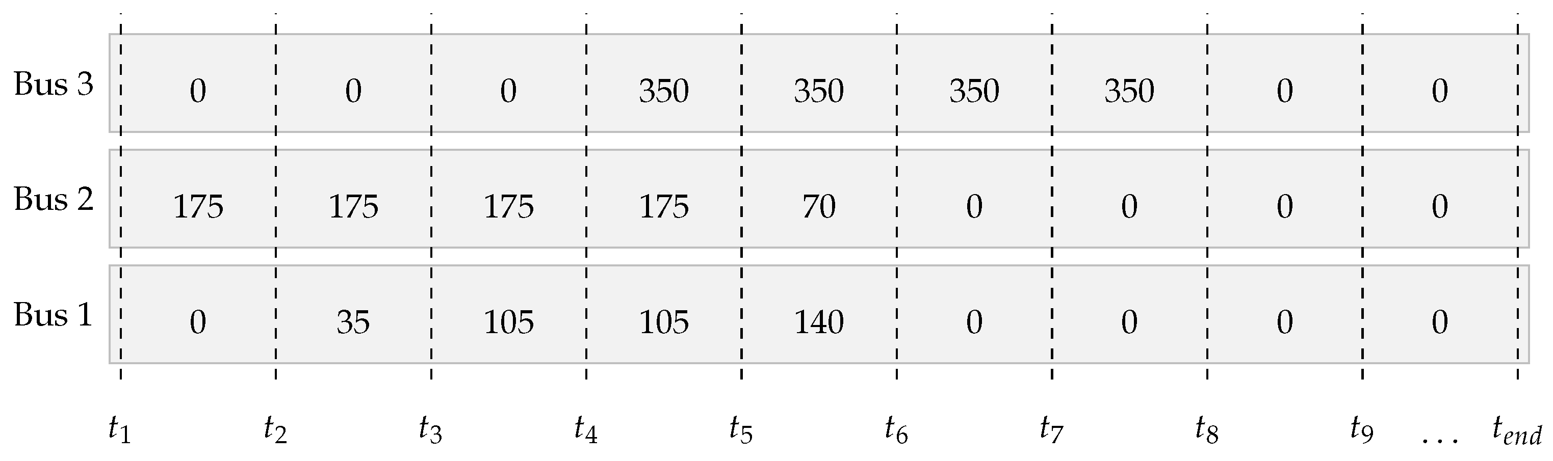
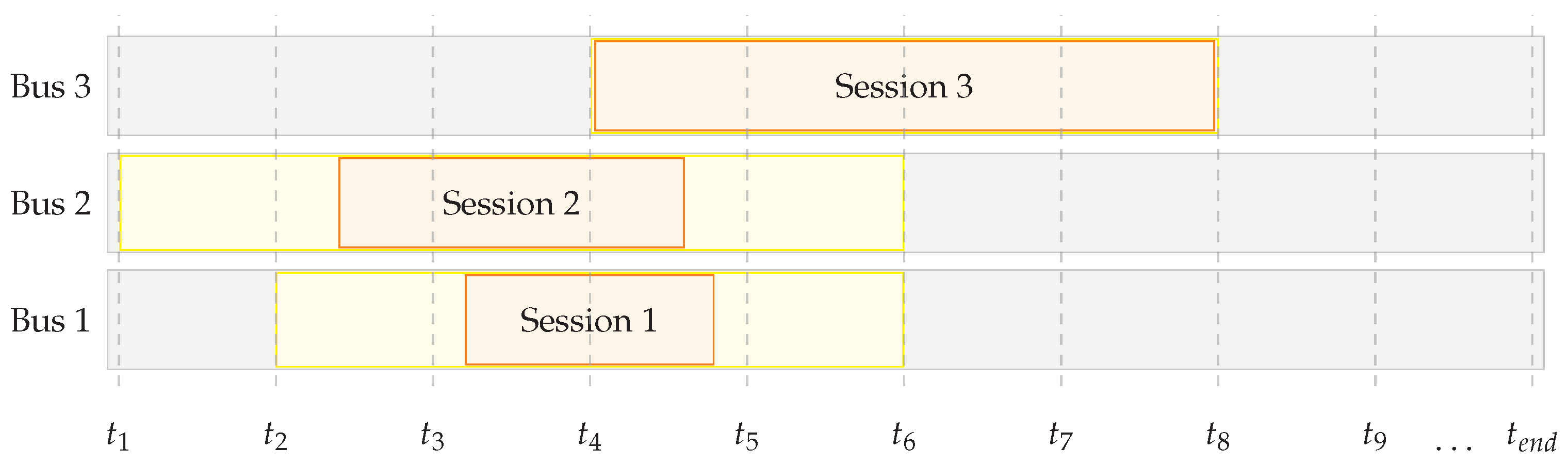
Consider a solution to a three-bus two-charger scenario provided in Figure 7. Note that there appear to be three buses charging at the same time from $t_5$ to $t_6$ even though there are only two chargers. We can reformulate this solution in terms of continuous start and stop variables and a variable charge rate so that the duration of each charge session may be relaxed. The objective is to transfer the required energy to the corresponding bus within the optimized charge interval.

Note how few of the charge sessions utilize the chargers to full capacity. This implies that there exists a smaller charge window in which equivalent power can be delivered. This allows us to use the charge durations from the solution from Figure 7 as bounds on allowable charge windows instead of enforcing equality.

An example of how Figure 7 may be reformulated is provided in Figure 8. Note how the actual charge sessions do not necessarily need to take up all the time they were initially allocated in the first solution and that these times can fluctuate if the average charge rate is less than the maximum charger capacity. In this example, we assume a maximum charge capacity of 350 kW.

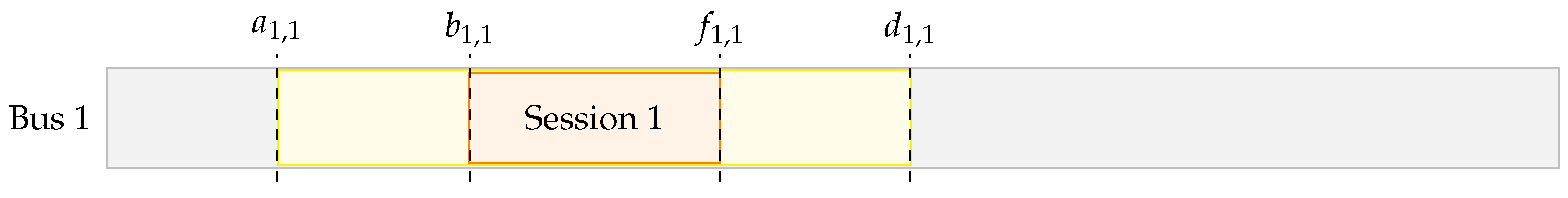
Note how the third charge session does have to be exactly where it was scheduled because the average is equal to the maximum charge rate. If we examine just the schedule for Bus 1, we note that there are four essential variables for the corresponding charge session: $a(i,r)$, $b(i,r)$, $f(i,r)$, and $d(i,r)$, which represent the minimum start time, actual start time, actual end time, and maximum end time, respectively.

The problem we must now solve is one of arranging these intervals such that each one is larger than its minimum width (or charge time). We must also account for the number of chargers. It can be helpful to view the problem as a bin packing problem, where each session must fit within the “swim lane” of a charger. For example, taking the charge sessions provided in Figure 8 and arranging them so that there is no overlap between sessions will yield a valid solution as shown in Figure 9. From Figure 10, we know that $a(i,r),b(i,r),f(i,r)$, and $d(i,r)$ must be such that

$$a(i,r)\le b(i,r)\le f(i,r)\le d(i,r),$$

(24)

where $a(i,r)$ and $d(i,r)$ are known from $P_4$, and $b(i,r)$ and $f(i,r)$ are optimization variables.

To differentiate between different chargers, define $\sigma (i,r,k)$ as a binary selector variable that is one if charger k services bus i for session r and zero otherwise. Because only one charger can charge each bus at a time and each charge session must be serviced, we have

$$\sum _k\sigma (i,r,k)=1\forall i,r.$$

(25)

Next, we also know that during each session a certain amount of energy must be transferred from the charger to the battery. The amount of energy that must be transferred to bus i during session r is provided in the solution to $P_4$ and denoted $e(i,r)$. We can compute a minimum time window from these values by letting

$$w{(i,r)}_{\min }=\frac{e(i,r)}{p_{\max }}.$$

(26)

If we include constraints for a minimum time per session, then the previous expression becomes

$$w{(i,r)}_{\min }=\max \left(w_{\min },\frac{e(i,r)}{p_{\max }}\right).$$

Because $w{(i,r)}_{\min }$ is the minimum time window, we must ensure that the difference between the start and stop times is at least this large so that

$$f(i,r)-b(i,r)\ge w(i,r)\forall i,r.$$

(27)

The final set of constraints deals with contention so that no charger can be scheduled for two sessions that overlap. Let $\mathcal{L}=\{(i,r)\times (i^{\prime },r^{\prime })\}$, where charge sessions $i,r$ and $i^{\prime },r^{\prime }$ have the potential to overlap. Before we can prevent overlap, we must define a binary variable $l(i,r,i^{\prime },r^{\prime })$ that is equal to one when session $i,r$ is scheduled before session $i^{\prime },r^{\prime }$ and zero otherwise so that

$$\left\{\begin{array}{cc}f(i,r)\le b(i^{\prime },r^{\prime })\hfill & l(i,r,i^{\prime },r^{\prime })=1\hfill \\ f(i^{\prime },r^{\prime })\le b(i^{\prime },r^{\prime })\hfill & l(i,r,i^{\prime },r^{\prime })=0\hfill \end{array}\right.$$

(28)

To simplify these constraints, let M have a large value such as the number of seconds in a day. We know what the top constraint must be trivially satisfied when $l(i,r,i^{\prime },r^{\prime })=0$ and the bottom must also when $l(i,r,i^{\prime },r^{\prime })=1$. This leads to a reformulation so that

$$\begin{array}{cc}\hfill f(i,r)-b(i^{\prime },r^{\prime })& \le M(1-l(i,r,i^{\prime },r^{\prime })\hfill \\ \hfill f(i^{\prime },r^{\prime })-b(i,r)& \le l(i,r,i^{\prime },r^{\prime })M\hfill \end{array}$$

However, this constraint only needs to hold when sessions $i,r$ and $i^{\prime },r^{\prime }$ are scheduled to charge on the same charger or $\sigma (i,r,k)=\sigma (i^{\prime },r^{\prime },k)=1$. We can reformulate the above constraint to satisfy this condition by letting

$$\begin{array}{cc}\hfill f(i,r)-b(i^{\prime },r^{\prime })& \le M(3-\sigma (i,r,k)-\sigma (i^{\prime },r^{\prime },k)-l(i,r,i^{\prime },r^{\prime }))\hfill \\ \hfill f(i^{\prime },r^{\prime })-b(i,r)& \le M(2-\sigma (i,r,k)-\sigma (i^{\prime },r^{\prime },k)+l(i,r,i^{\prime },r^{\prime }))\hfill \end{array}$$

(29)

Finally, we desire the schedule to closely match the charge plan from $P_4$, which occurs when each charge session matches the durations provided in $P_4$, so we formulated an objective function that minimizes the differences in the given plan and the results from $P_4$ by letting the objective be

$$\underset{f,b}{\min }\sum _{i,r}{\parallel b(i,r)-a(i,r)\parallel }_2^2+{\parallel f(i,r)-d(i,r)\parallel }_2^2$$

(30)

which has the effect of driving each variable to the desired value and more heavily penalizing values that are further from their optimal. The final optimization problem is provided below.

Ideally, when $P_5$ is solved to optimality, the chargers are fully utilized. However, optimality for $P_5$ is computationally demanding and scalable solutions may require relaxations in the optimality gap of the solver. However, increasing the gap leads to a solution in which chargers are not fully utilized. The next section uses the session ordering from $P_5$ but recomputes session start/stop times to better utilize the charger availability even when sub-optimal gaps are provided for $P_5$.

2.2.3. Optimizing Charge Schedules ($P_6$)

Often, it is not feasible to compute the optimal set of charge schedules provided in the previous sections. As the amount of buses and charge sessions becomes large, computing a small-gap solution becomes computationally intractable. Allowing solutions with larger optimality gaps decreases the number of computations but results in sub-optimal charge-time windows. In this section, a more optimal set of charge windows is computed using the results from $P_5$ to infer charger assignment and ordering for each charge session. We also know that the optimal solution will expand the charge windows to use any available time where a charger is unused, implying that the “stop” time for each session will either be equal to its bus’s departure time or the start time of the next window, which can be expressed as

$$\left\{\begin{array}{cc}c(s,i,r+1)=c(f,i,r)\hfill & c(d,i,r)>c(a,i,r+1)\hfill \\ \begin{array}{cc}\hfill c(s,i,r+1)& =c(a,i,r+1)\hfill \\ \hfill c(f,i,r)& =c(d,i,r)\hfill \end{array}\hfill & c(d,i,r)<=c(a,i,r+1)\hfill \end{array}\right.$$

(31)

where $c(s,i,r)$ is the start time for charger i’s $r\mathrm{th}$ charge session, $c(f,i,r)$ is the stop time for charger i’s $r\mathrm{th}$ charge session, $c(d,i,r)$ is the departure time for the bus scheduled for charger i’s $r\mathrm{th}$ charge session, and $c(a,i,r)$ is the arrival time for the bus scheduled for charger i’s $r\mathrm{th}$ charge session. The minimum charge length must also be used so that energy can be properly delivered, so that

$$c(f,i,r)-c(s,i,r)\ge w(i,r)$$

(32)

where $w(i,r)$ is the minimum charge time for the corresponding session.

The final step to optimizing the charge windows is to assign preference to windows with larger power deliveries. Let the objective for the optimization program be

$$J_{\mathrm{window}}=\frac{1}{n}\sum _{i,r}{∥\frac{c(f,i,r)-c(s,i,r)}{e(i,r)}∥}_2^2.$$

(33)

When the function J contains windows with equal amounts of energy, the minimum will be found where each charge interval is the same width. As the amount of energy increases, the objective penalizes less for larger window sizes and thus assigns preference to high-energy sessions. The final optimization problem is provided below.

After solving $P_6$, each charge session is assigned to a charger so that contention for limited chargers has been managed for each group. Furthermore, each session also specifies target energy requirements that manage the risks of depleting batteries but do not provide instructions on how the energy is to be delivered. The energy delivery problem is addressed in the next section and the results are combined for all groups so that the charge schedule begins to approach a globally optimal solution.

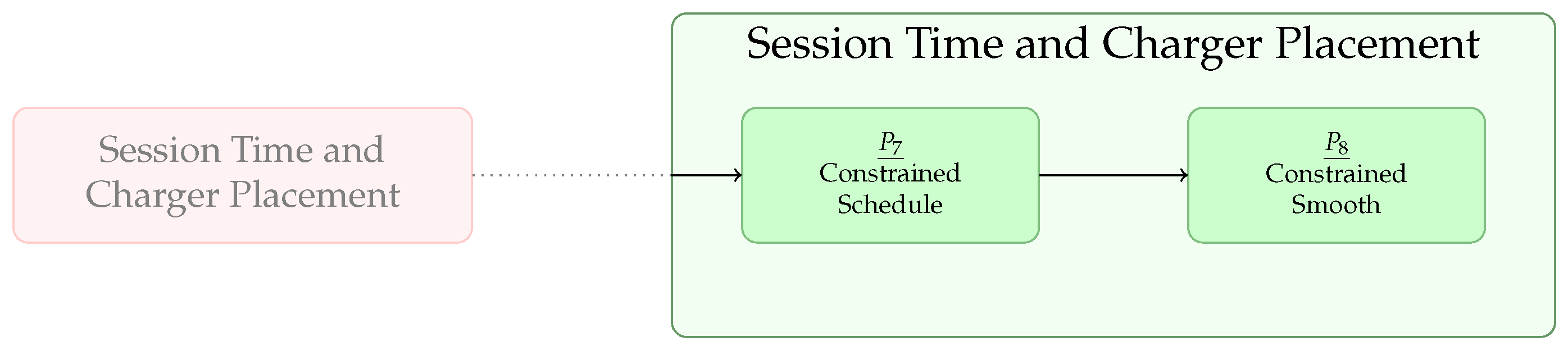
2.3. Final Optimization

Solutions to the previous problems provide a set of charge sessions, energy requirements, and time schedules for specific chargers. The final question to be answered is how should the energy for each session be delivered. The two subproblems in the final optimization section mirror problems $P_1$ and $P_2$ from the energy allocation and group assignment sections. The first problem (denoted $P_7$) uses the energy and time constraints from previous solutions to compute an optimal charge schedule in Section 2.3.1 and is analogous to the unconstrained charge problem $P_1$. The second problem (denoted $P_8$) computes a smoothed charge schedule with the same cost as the constrained schedule solution in Section 2.3.2 and is analogous to the smooth charge schedule problem $P_2$ in Section 2.1.2. Together, $p_7$ and $p_8$ form the third set of optimization problems as shown in Figure 11.

2.3.1. Constrained Schedule ($P_7$)

Up to this point, we have computed charge schedules that assume that any bus can charge regardless of the number of chargers. We then separate buses into groups to reduce the scale of the problem and treat each subproblem separately while we defragment sessions and assign each charge session to specific chargers before determining the final start and stop times for each bus’s charge session.

The final step in this process is to determine how the energy will be delivered so that cost is minimized. We begin with constraints for bus power, energy, and cost from Section 2.1.1 that are expressed as Equations (1), (5), and (7)–(11). Next, include constraints for energy so that the energy for each charge session is properly delivered using a modified version of (22) so that

$$\mathbf{b}(i,:)\rho (i,r)=\psi (i,r),$$

(34)

where $\psi (i,r)$ is the required energy for bus i during rest period r as computed from the solution of the defragmentation problem. The resulting optimization problem is provided below.

2.3.2. Constrained Smooth Schedule ($P_8$)

The charge schedule from $P_7$ will contain the same on–off switching defects as the solution to $P_1$, which can be managed as before by executing $P_7$ once again with the same modifications that lead to $P_2$: (1) constrain the cost terms in the objective to equal their values from $P_7$, and (2) reduce the difference in sequential charge rates with the smoothing objective from (14). The resulting optimization problem is provided below.

3. Results

The results provided in this section aim to demonstrate how the proposed method can be used to find a scalable solution to the bus charge problem. Because the proposed solution contains various subproblems, optimization parameters for each subproblem may be tuned to best meet the demands of a given scenario, allowing for a degree of flexibility that is not present in prior works that formulate solutions to the bus charge problem as a single optimization problem.

3.1. Overall Performance

In this section, we compare the proposed method with a baseline algorithm and a method developed by [27]. The baseline method models how bus drivers charge their electric vehicles at the Utah Transit Authority (UTA) in Salt Lake City, Utah. At the UTA, when bus drivers arrive at the station, they recharge their batteries whenever a charger is available so that the number of charge sessions is maximized. The method from [27] works somewhat differently by minimizing the cost of energy with respect to time of use tariffs ${\mu }_{e-on}$ and ${\mu }_{e-off}$.

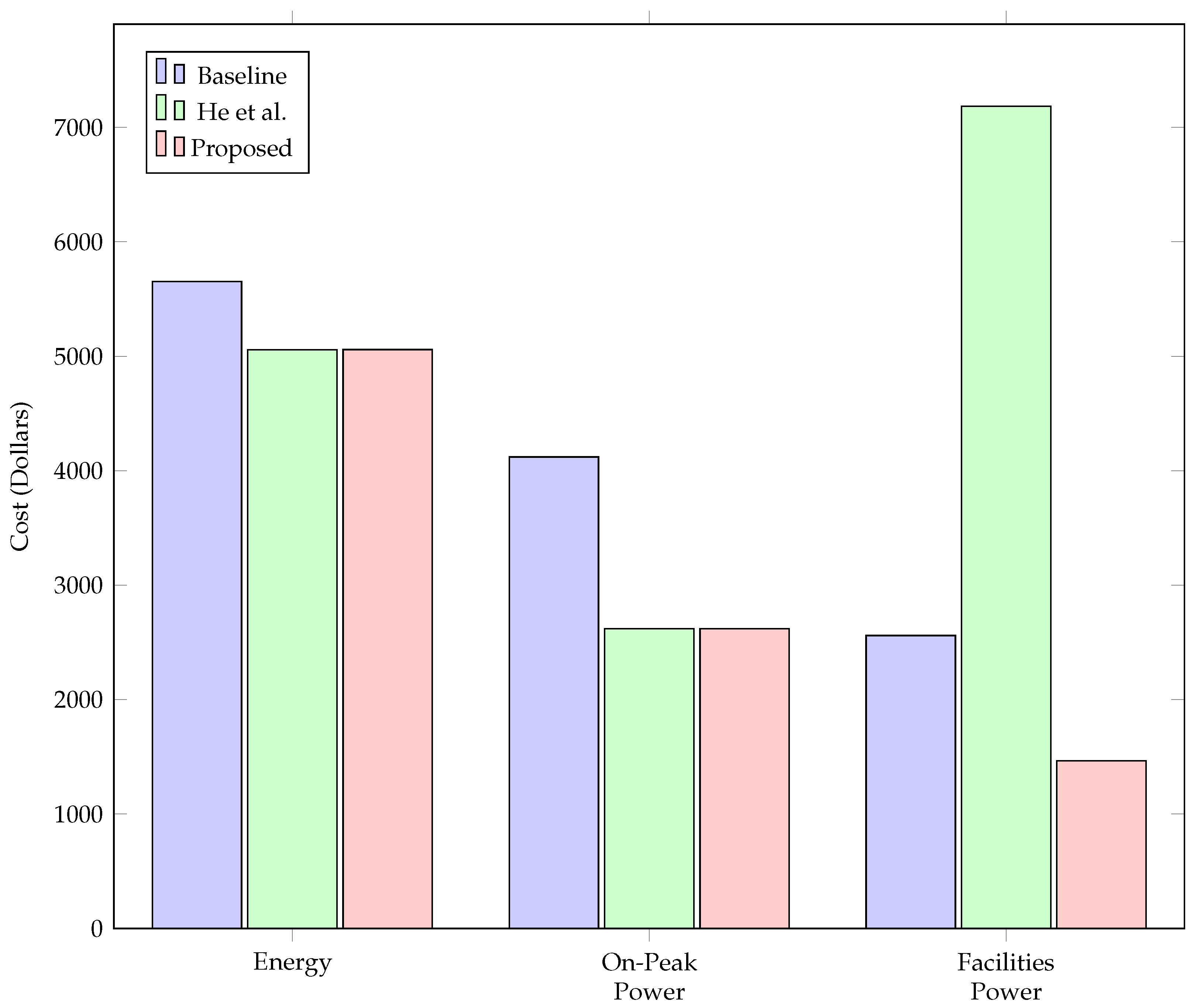
The comparison we observe is provided for a 10-bus 10-charger scenario and a single group. Each method was used to compute a charge schedule, and the costs from demand, facilities, and energy charges are provided in Figure 12. Note how the baseline algorithm suffers significantly from the demand charges associated with on-peak power, and [27] incurs additional costs from facilities charges, indicating that the emphasis on energy charges and habitual charging patterns can be improved.

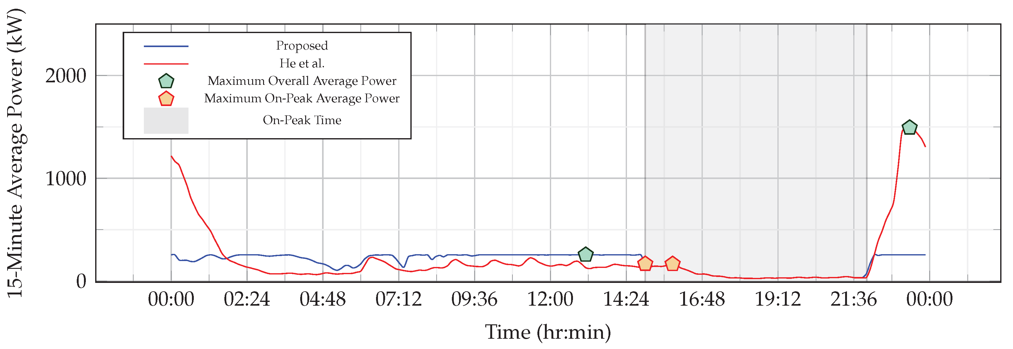
We observe where the differences in cost originate in Figure 13. Observe how the baseline charge profile achieved the largest 15 min average power between 19:12 and 21:36, which is during on-peak hours, and consequently yielded the large on-peak power charges provided in Figure 12. Additionally, note how the proposed method maintains a relatively flat power profile so that the load is balanced throughout the day, which we investigate in Figure 14.

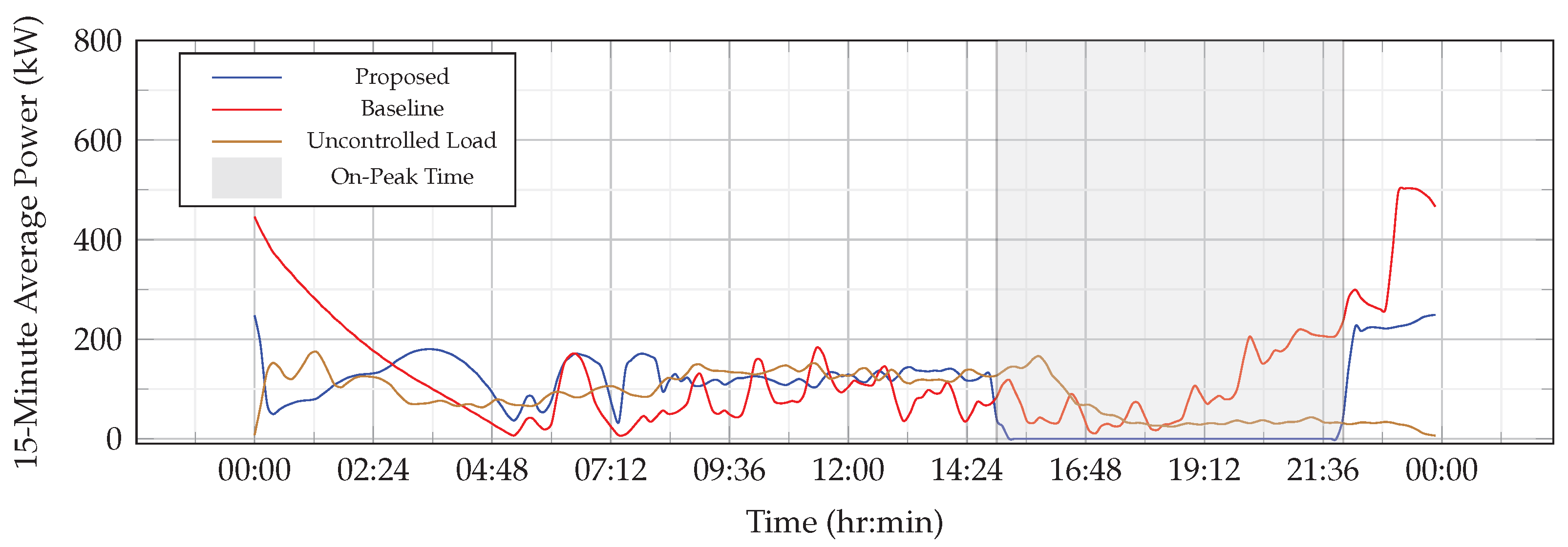
In Figure 14, note how the proposed method produces a bus load that mirrors the uncontrolled load, yielding the flat load profile from Figure 13, which is especially prevalent from 7:12 to 14:24. The results show that the proposed method works well, outperforming both the historical patterns at UTA as well as improving upon prior methods.

3.2. Optimality Gap and Contention Trade-Off

In the previous section, we compared the performance of three methods where each method was produced using a small gap in the numerical solver. In general, the most computationally demanding solution addressed bus-to-charger placement and can require a very small gap to yield good solutions.

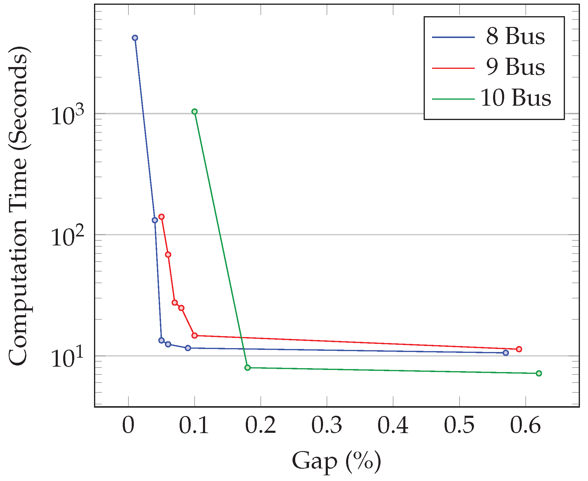
This work also seeks to address how to compute a solution in a scalable manner, so this section reviews the relationship between computation time and number of buses by considering a seven-charger scenario with runtime comparisons for eight, nine, and ten buses.

Figure 15 plots the computation time as a function of optimality for a seven-charger eight-bus scenario in blue, a seven-charger nine-bus scenario in red, and a seven-charger ten-bus scenario in green. In each scenario, note how there exists a gap after which computation time dramatically increases for small improvements in the optimality gap. Solving $P_5$ to an optimality gap after this point becomes computationally expensive and should be avoided as the number of buses grows.

Additionally, note how the high solve-time region (near zero gap) for the eight-bus scenario begins at a smaller gap than that of the nine- or ten-bus scenarios. This demonstrates a relationship between contention and computation time as contention increases with the number of buses if the number of chargers is fixed. We can conclude, therefore, that saving computation time as the number of buses increases can be accomplished by slackening (increasing) the optimality gap provided to the numerical solver.

3.3. Contention: Sub-Optimal Schedules

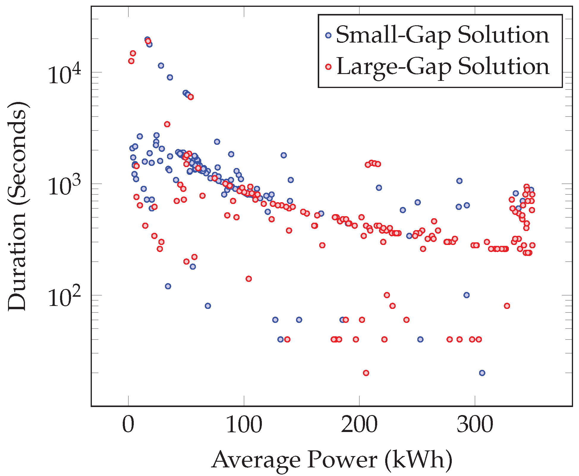
In the previous section, we observed that the proposed method cannot scale with contention if the optimality gap is too small. This section considers an experiment to motivate the division into groups from $P_3$. The focus of this experiment is to compare the duration and charge rates of small-gap and large-gap scenarios. Solutions to $P_5$ are preferred if session lengths are longer and require smaller charge rates because long charge sessions are more practical in the real world and small charge rates are easier to implement on charging hardware.

Figure 16 displays the charge session durations as a function of charge rate for two solutions to an eighteen-bus six-charger scenario. The first solution, shown in blue, was computed with a small optimality gap and the second, shown in red, was computed for a large optimality gap. Note how the charge sessions from the small-gap solution tend to have larger session durations and lower charge rates than the solution for the large-gap sessions, indicating the value of smaller gaps.

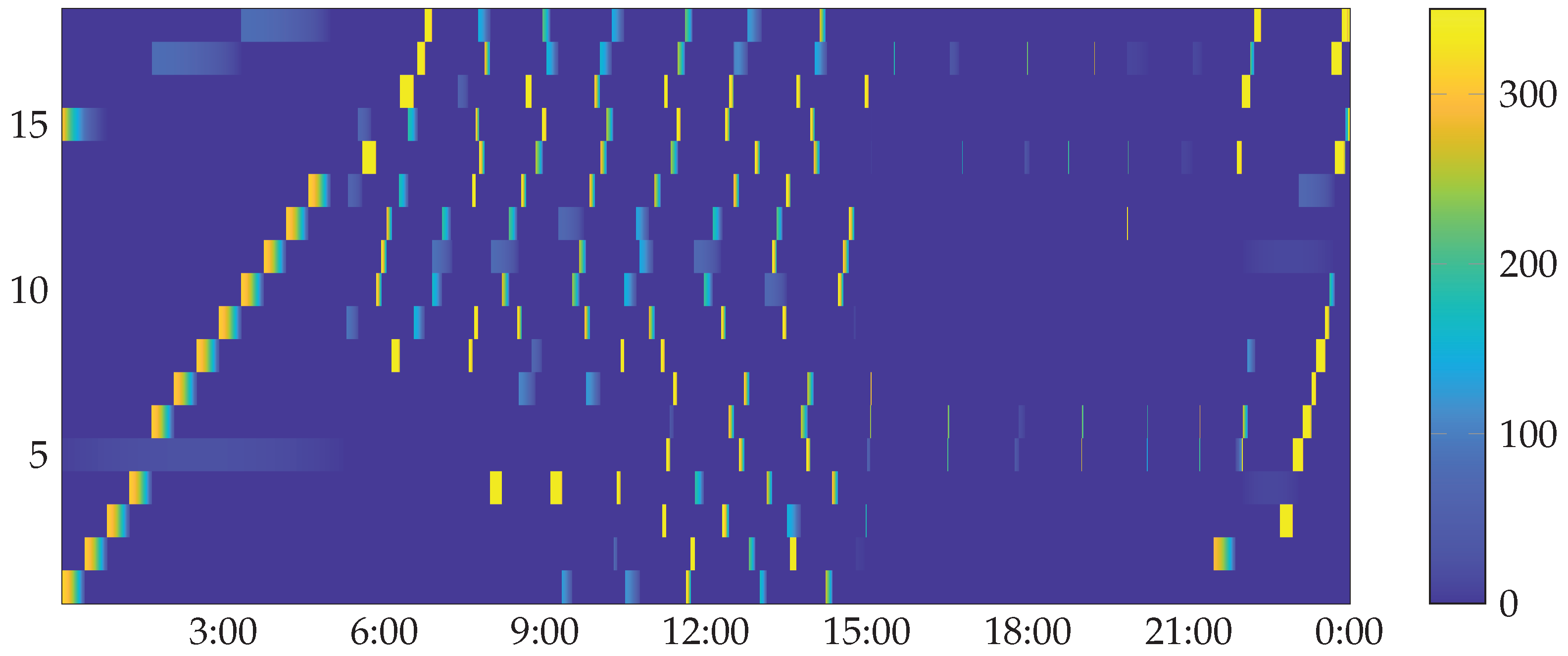
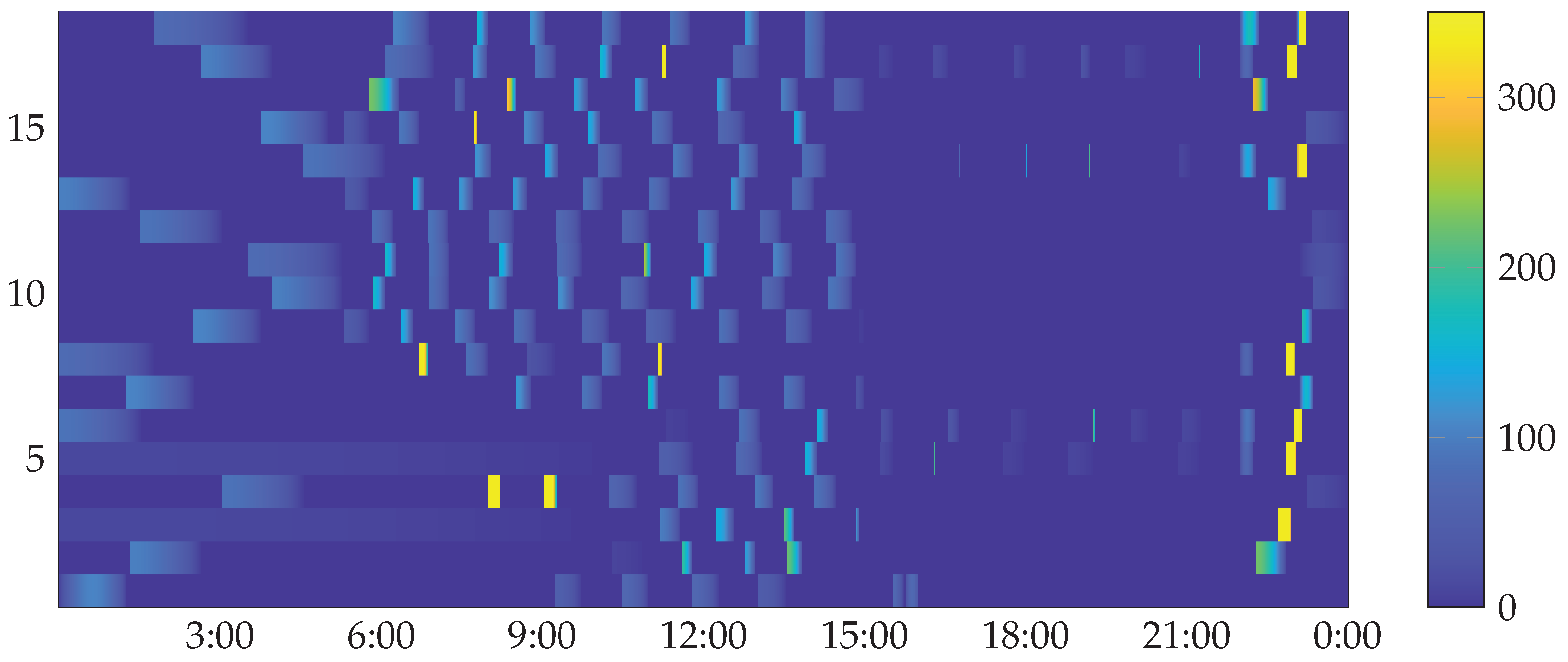
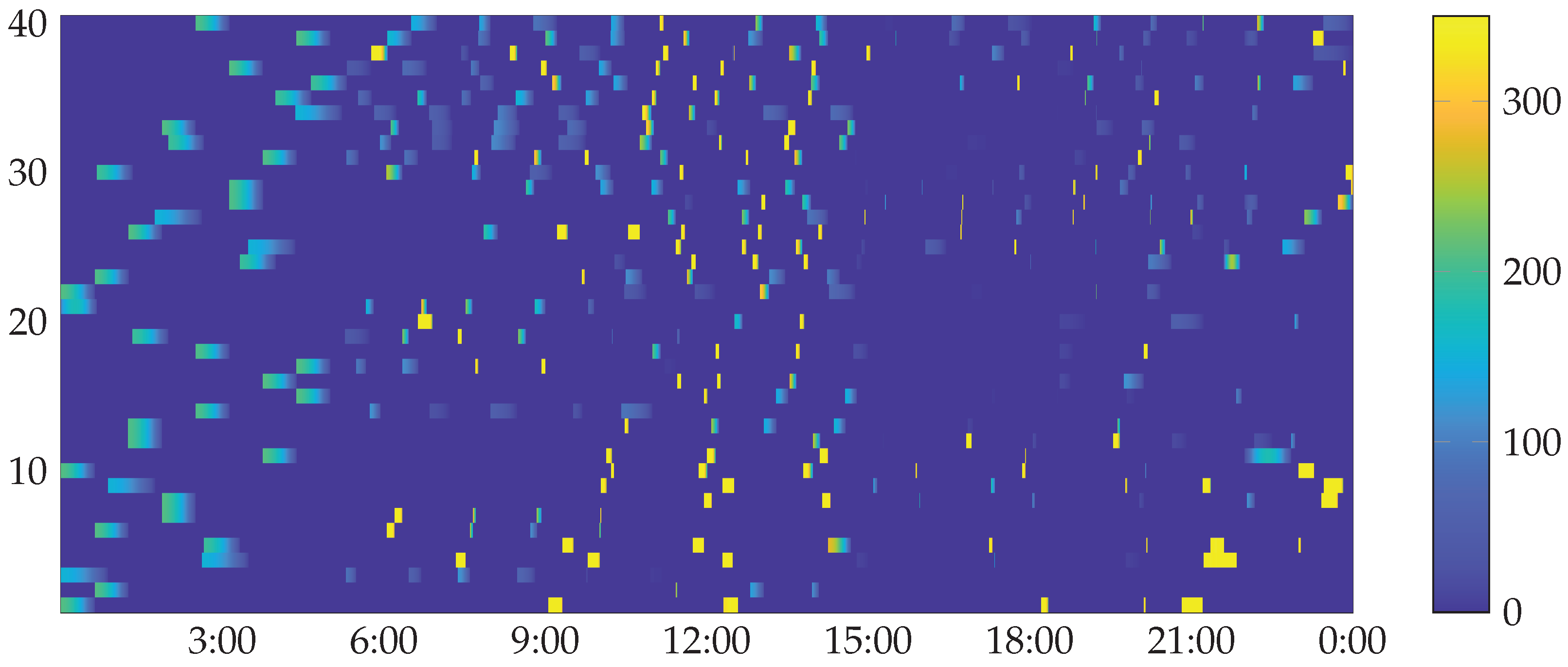
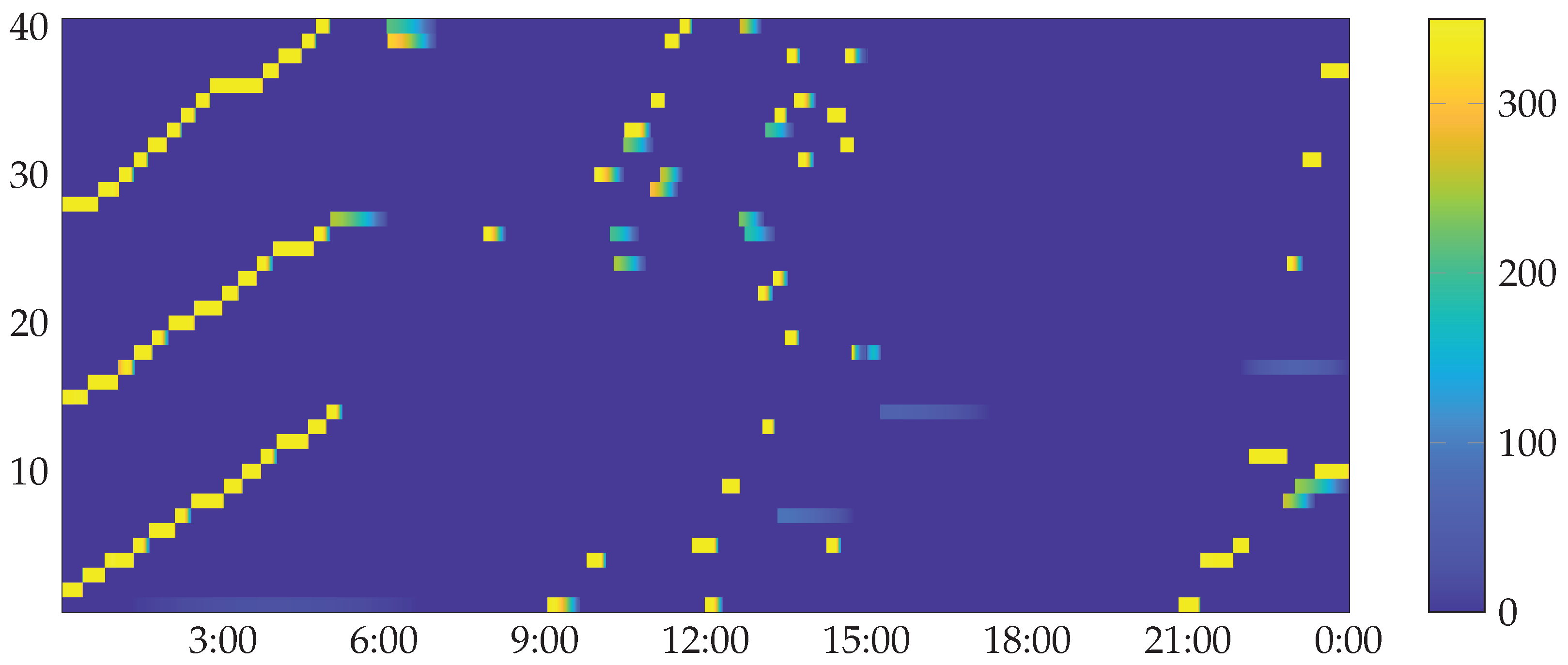
We further illustrate the difference in optimality gap by directly comparing the charge schedules for each scenario in Figure 17 and Figure 18. In each figure, the color at the $i,j$ location represents the charge rate for bus i at time j. Observe how the first sessions for buses 1–4 and 6–13 are assigned to a single charger in Figure 17 so that each charge session is compressed to accommodate the large number of buses. The remaining chargers appear to have at most one session, which implies that the charge sessions were poorly managed in the large-gap scenario. In comparison, the small-gap solution in Figure 18 yields a more evenly distributed session load for each charger so that each session is lengthened and contains smaller charge rates.

It is also interesting to note that the monthly costs of each solution may or may not be equivalent even though a small-gap solution is clearly superior. Therefore, a small gap is required to consistently achieve optimal session placement. We also know from Figure 15 that small optimality gaps may increase the number of computations so that the charger assignment problem becomes intractable for large numbers of buses, making it necessary to reduce the problem scope by dividing buses into groups.

3.4. The Importance of Groups

One contribution this work provides is a way to compute cost-oriented charge schedules that scale well as the number of buses increases. We know from the previous section that the charger assignment problem will not scale for small optimality gaps. This section describes how the computational complexity of the charger assignment problem can be managed by separating the buses into groups so that the charger assignment problem can be solved for each group independently.

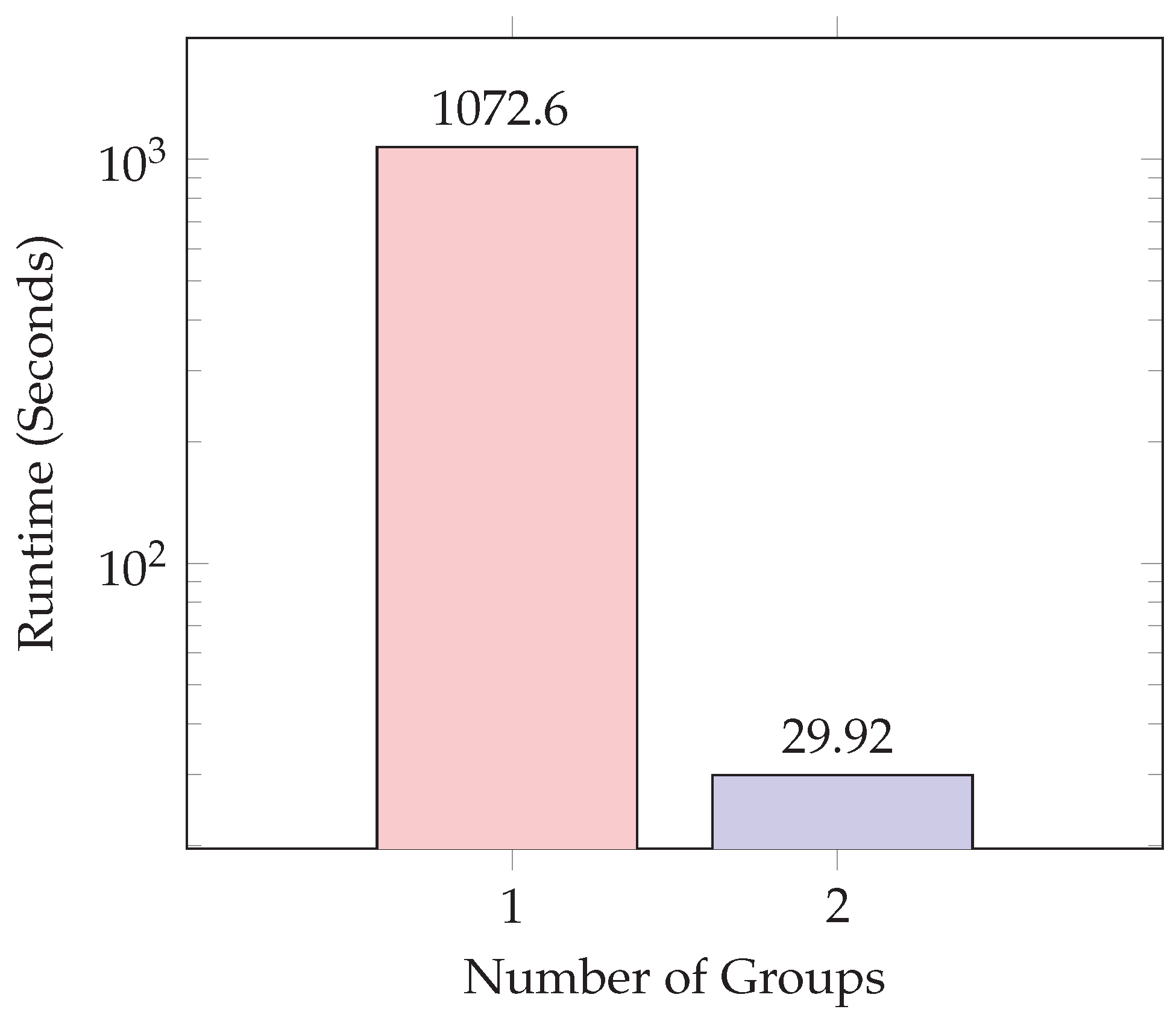
In this section, we consider an 18-bus 12-charger scenario with a 0.13% gap in the charger assignment problem. Figure 19 shows the respective runtimes for one- and two-group scenarios in $P_5$. Note how the runtime for the two-group scenario is several orders of magnitude less than the runtime for the single-group case, which demonstrates how a small number of groups can manage the runtime for optimal charger assignment solutions.

3.5. Effects of Defragmentation

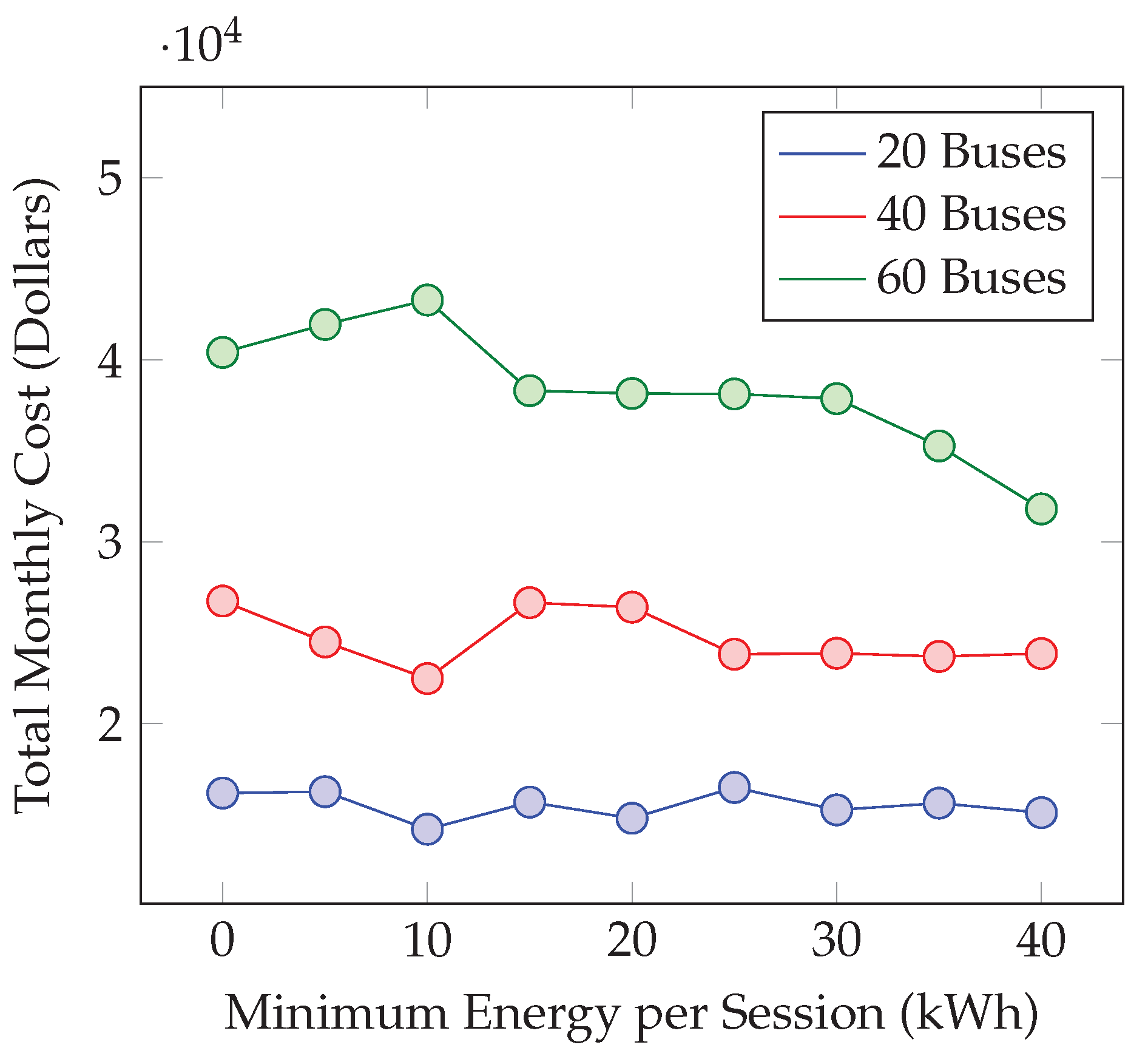
This paper also addresses the operational preference to consolidate charge sessions when possible, an operation we have called defragmentation. This section demonstrates the effectiveness of the defragmentation method provided in $P_4$ and how consolidation affects the monthly cost. In Section 2.2.1, the threshold for defragmentation is provided by the minimum allowable energy per charge session. In this section, we compare two forty-bus seven-charger scenarios where the first contains results without defragmentation and the second consolidates charge sessions so that each session delivers at least 30 kWh. The results for each session are presented in Figure 20 and Figure 21, where the color of the $i,j$ element of a figure represents the charge rate for bus i during time j. Note how Figure 20 contains many short inconsequential charge sessions and requires each bus to charge each time it enters the station. In comparison, Figure 21 contains only a handful of charge sessions so that each bus only needs to charge four to five times throughout the day.

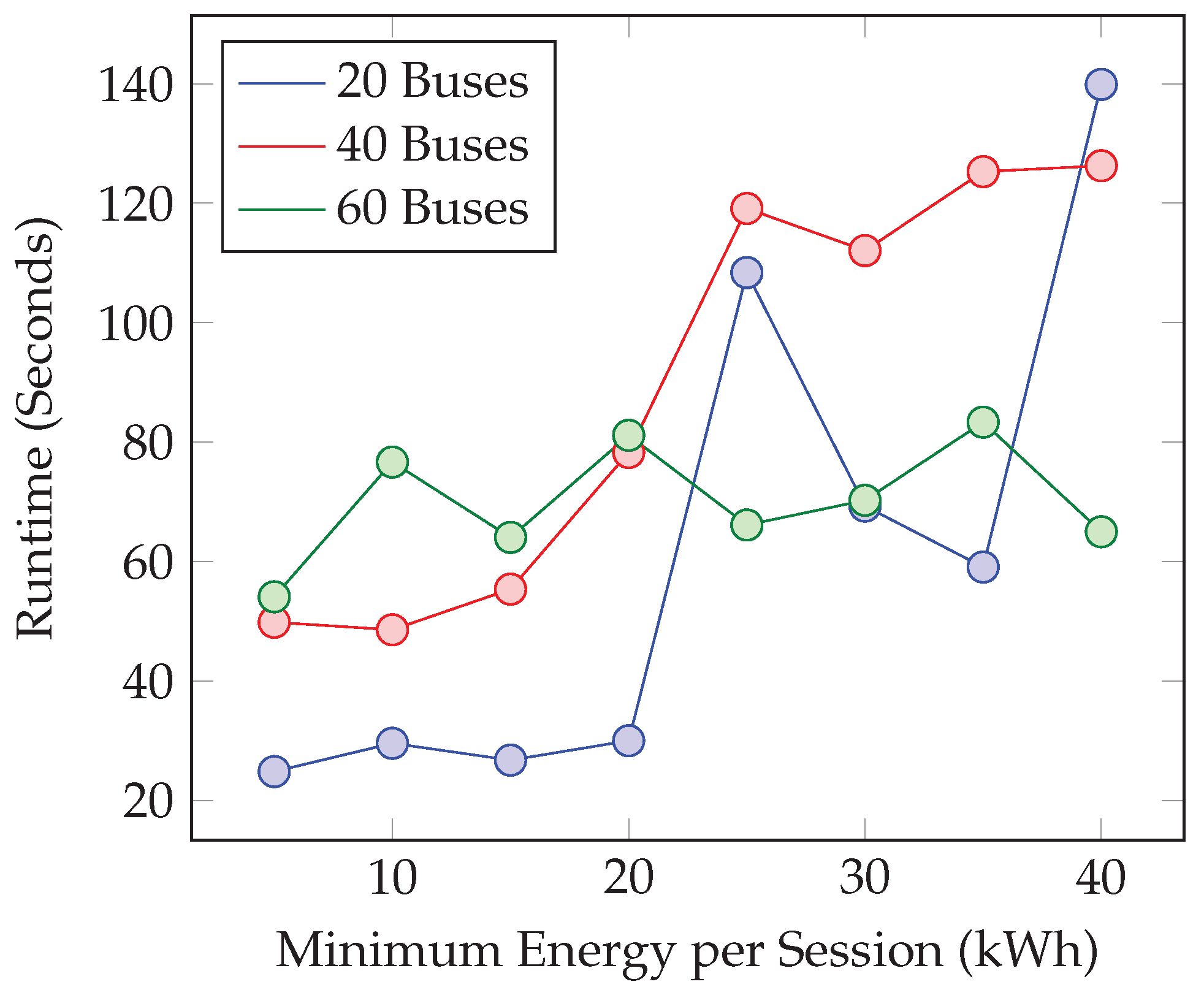
Furthermore, Figure 22, which plots monthly cost as a function of the minimum charging threshold, demonstrates that, despite the additional constraints associated with consolidation, the monthly cost remains consistent over a large window of thresholds. As the minimum allowable energy per session increases, the number of binary variables in the defragmentation problem increases, resulting in significant runtimes for the defragmentation problem as shown in Figure 23, which plots runtime as a function of the minimum charge threshold. However, because buses are divided into groups prior to defragmentation, the smaller groups decrease the computational complexity for defragmentation so that larger consolidation thresholds can be applied in a scalable manner.

3.6. Scalability

In this section, we consolidate what we have learned in the previous sections to demonstrate how the proposed framework can be used to compute a cost-effective solution for large numbers of buses. This section focuses on a scenario with a minimum energy per session of 20 kWh, a large gap for the charger assignment solution, and a single group.

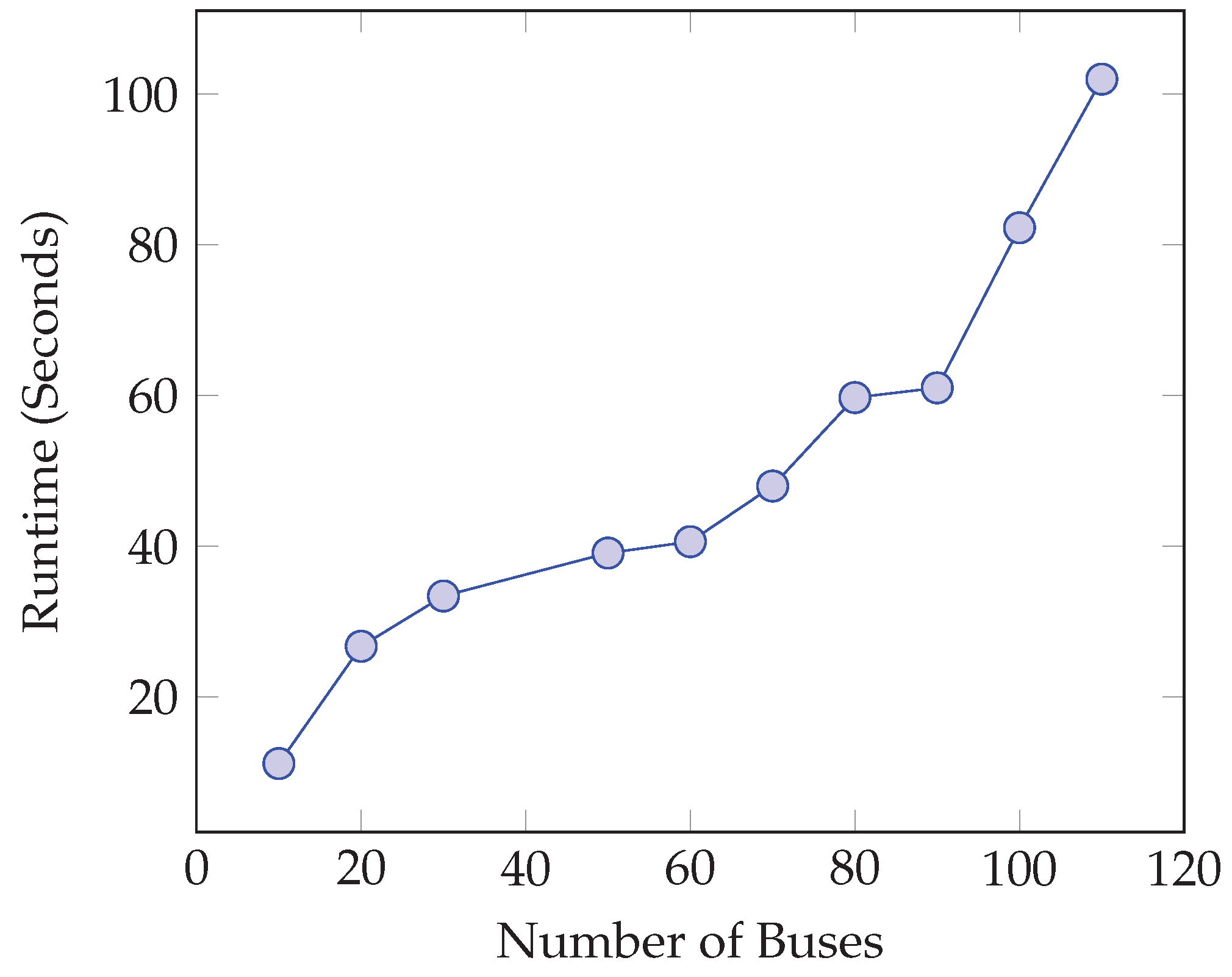
The results are provided in Figure 24, which plots the runtime as a function of the number of buses and shows how that runtime generally increases by one second per bus from 10 to 110 buses. One would expect the runtime to increase at least in the order of $O\left(n^2\right)$ for a globally optimal solution because of the coupling between bus variables. The fact that the proposed method is practical in the given range indicates a solution that scales well as the number of buses increases and can easily handle over 100 buses.

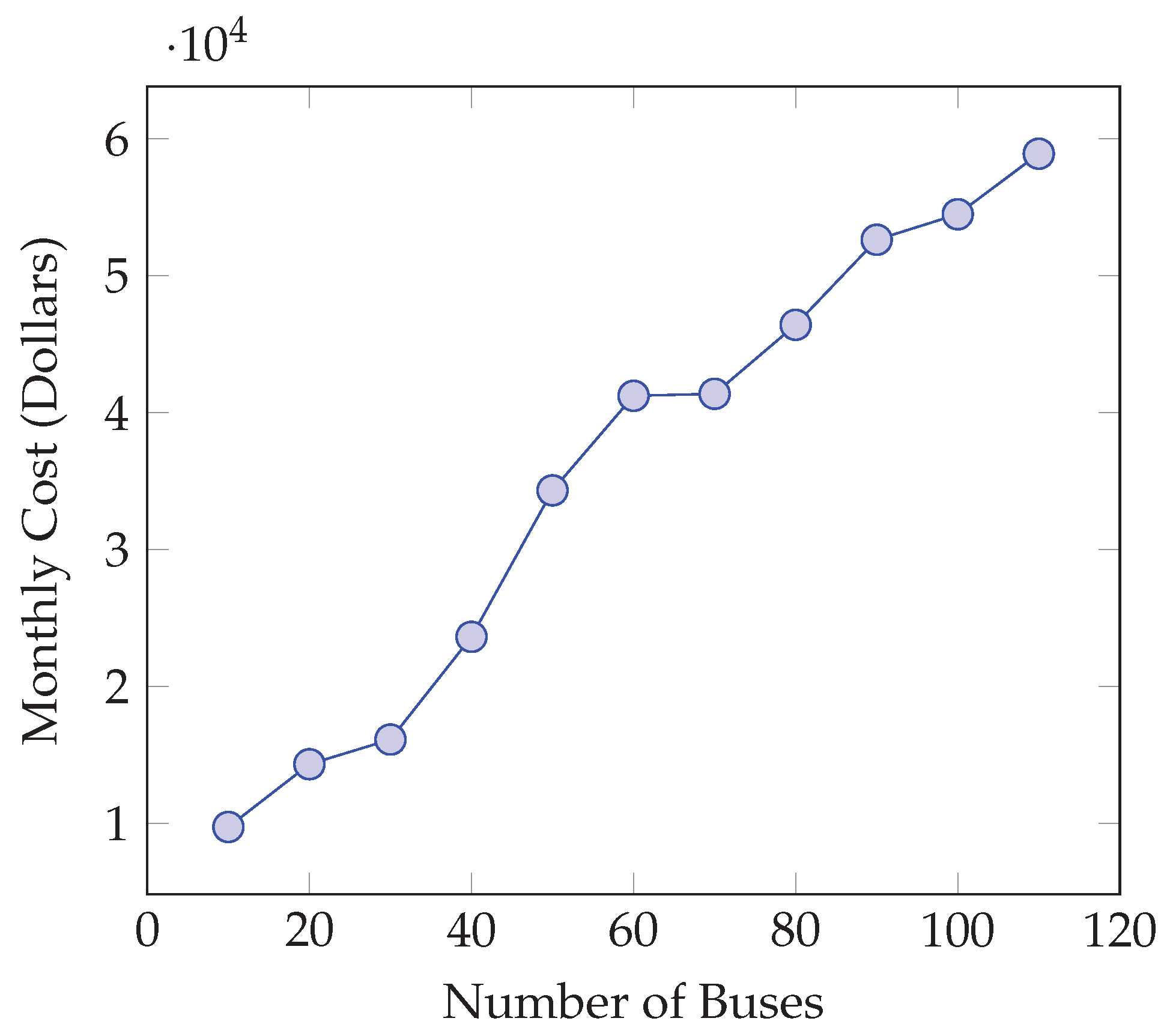
Generally, one would also expect such savings to come with significant increases to monthly cost. However, the results in Figure 25 demonstrate that the proposed solution yields a quasi-linear increase of approximately USD 404.10 per bus per month.

4. Conclusions

In summary, this paper set out to compute a cost-oriented charge plan for large bus fleets. Historical methods have focused on either scalability or optimality. Work with an optimality-centered focus has not scaled to large bus fleets because the number of variables in such formulations becomes very large as the number of buses increases. Others have worked with compute time in mind but have been unable to consider details that lead to optimal schedules.

We have shown how the proposed method can do both, considering the details in a BEB’s day-to-day use that allow for optimal schedules and providing the user with hyper-parameters that allow them to decide how optimal their solution must be. The bus charge problem has been divided into a series of programs that use information from the previous program to further refine the charge schedule. The hyper-parameters in this formulation are the optimality gap criteria for each subprogram.

The primary constraints this paper considers are time of use and demand charge, bus and charger availability, the state of charge and maximum capacity of a BEB’s battery, fragmented charge sessions, bus grouping, and second-by-second optimization.

We consider the results for each subproblem in Section 3 and demonstrate that the proposed method can scalably plan for large bus fleets, achieving a cost of approximately USD 400.00 per month per bus, and a runtime of one second per bus (up to 110 buses). The proposed method’s ability to consider many operational details and manage compute time makes the proposed method ideal for managing the cost of energy in large electric bus fleets. Furthermore, using a variety of programs to solve the bus charge problem guarantees that all the solutions will not only be cost-effective but feasible as well.

References

- Mahmoud, M.; Garnett, R.; Ferguson, M.; Kanaroglou, P. Electric buses: A review of alternative powertrains. Renew. Sustain. Energy Rev. 2016, 62, 673–684. [Google Scholar] [CrossRef]
- Poornesh, K.; Nivya, K.P.; Sireesha, K. A Comparative study on Electric Vehicle and Internal Combustion Engine Vehicles. In Proceedings of the 2020 International Conference on Smart Electronics and Communication (ICOSEC), Trichy, India, 10–12 September 2020; pp. 1179–1183. [Google Scholar] [CrossRef]
- Kato, H.; Ando, R.; Kondo, Y.; Suzuki, T.; Matsuhashi, K.; Kobayashi, S. Comparative measurements of the eco-driving effect between electric and internal combustion engine vehicles. In Proceedings of the 2013 World Electric Vehicle Symposium and Exhibition (EVS27), Barcelona, Spain, 17–20 November 2013; pp. 1–5. [Google Scholar] [CrossRef]
- Cheng, Q.; Chen, L.; Sun, Q.; Wang, R.; Ma, D. A smart charging algorithm-based fast charging station with energy storage system-free. Csee J. Power Energy Syst. 2021, 7, 850–861. [Google Scholar] [CrossRef]
- Nimalsiri, N.I.; Mediwaththe, C.P.; Ratnam, E.L.; Shaw, M.; Smith, D.B.; Halgamuge, S.K. A Survey of Algorithms for Distributed Charging Control of Electric Vehicles in Smart Grid. IEEE Trans. Intell. Transp. Syst. 2020, 21, 4497–4515. [Google Scholar] [CrossRef]
- Zhou, Y.; Liu, X.C.; Wei, R.; Golub, A. Bi-Objective Optimization for Battery Electric Bus Deployment Considering Cost and Environmental Equity. IEEE Trans. Intell. Transp. Syst. 2021, 22, 2487–2497. [Google Scholar] [CrossRef]
- Rinalde, M.; Picarelli, E.; D’Ariano, A.; Viti, F. Mixed-fleet single-terminal bus scheduling problem: Modeling, solution scheme and potential applications. Omega 2020, 96, 102070. [Google Scholar] [CrossRef]
- Houbbadi, A.; Redondo-Iglesias, E.; Trigui, R.; Pelissier, S.; Bouton, T. Optimal Charging Strategy to Minimize Electricity Cost and Prolong Battery Life of Electric Bus Fleet. In Proceedings of the IEEE Vehicle Power and Propulsion Conference, Hanoi, Vietnam, 14–17 October 2019; pp. 1–6. [Google Scholar] [CrossRef]
- Leou, R.C.; Hung, J.J. Optimal Charging Schedule Planning and Economic Analysis for Electric Bus Charging Stations. Energies 2017, 10, 483. [Google Scholar] [CrossRef]
- Wei, R.; Liu, X.; Ou, Y.; Fayyaz, S.K. Optimizing the spatio-temporal deployment of battery electric bus system. J. Transp. Geogr. 2018, 68, 160–168. [Google Scholar] [CrossRef]
- Jeong, S.Y.; Park, J.H.; Hong, G.P.; Rim, C.T. Automatic Current Control by Self-Inductance Variation for Dynamic Wireless EV Charging. In Proceedings of the IEEE Workshop on Emerging Technologies: Wireless Power Transfer (Wow), Montreal, QC, Canada, 3–7 June 2018; pp. 1–5. [Google Scholar] [CrossRef]
- Csonka, B. Optimization of Static and Dynamic Charging Infrastructure for Electric Buses. Energies 2021, 14, 3516. [Google Scholar] [CrossRef]
- Stahleder, D.; Reihs, D.; Ledinger, S.; Lehfuss, F. Impact Assessment of High Power Electric Bus Charging on Urban Distribution Grids. In Proceedings of the IEEE Industrial Electronics Society, Lisbon, Portugal, 14–17 October 2019; Volume 1, pp. 4304–4309. [Google Scholar] [CrossRef]
- Deb, S.; Kalita, K.; Mahanta, P. Impact of electric vehicle charging stations on reliability of distribution network. In Proceedings of the IEEE International Conference on Technological Advancements in Power and Energy, Kollam, India, 21–23 December 2017; pp. 1–6. [Google Scholar] [CrossRef]
- Boonraksa, T.; Paudel, A.; Dawan, P.; Marungsri, B. Impact of Electric Bus Charging on the Power Distribution System a Case Study IEEE 33 Bus Test System. In Proceedings of the IEEE PES GTD Grand International Conference and Exposition Asia, Bangkok, Thailand, 19–23 March 2019; pp. 819–823. [Google Scholar] [CrossRef]
- Ojer, I.; Berrueta, A.; Pascual, J.; Sanchis, P.; Ursua, A. Development of energy management strategies for the sizing of a fast charging station for electric buses. In Proceedings of the IEEE International Conference on Environment and Electrical Engineering, Madrid, Spain, 9–12 June 2020; pp. 1–6. [Google Scholar] [CrossRef]
- Qin, N.; Gusrialdi, A.; Paul Brooker, R.; T-Raissi, A. Numerical analysis of electric bus fast charging strategies for demand charge reduction. Transp. Res. Part A Policy Pract. 2016, 94, 386–396. [Google Scholar] [CrossRef]
- Whitaker, J.; Droge, G.; Hansen, M.; Mortensen, D.; Gunther, J. A Network Flow Approach to Battery Electric Bus Scheduling, in review. IEEE Trans. Intell. Transp. Syst. 2022, 24, 9098–9109. [Google Scholar] [CrossRef]
- Mortensen, D.; Gunther, J.; Droge, G. Cost Minimization for Charging Electric Bus Fleets. World Electr. Veh. J. 2023, 14, 351. [Google Scholar] [CrossRef]
- Wang, G.; Xie, X.; Zhang, F.; Liu, Y.; Zhang, D. BCharge: Data-Driven Real-Time Charging Scheduling for Large-Scale Electric Bus Fleets. In Proceedings of the Real-Time Systems Symposium, Nashville, TN, USA, 11–14 December 2019; pp. 45–55. [Google Scholar] [CrossRef]
- Bagherinezhad, A.; Palomino, A.D.; Li, B.; Parvania, M. Spatio-Temporal Electric Bus Charging Optimization With Transit Network Constraints. IEEE Trans. Ind. Appl. 2020, 56, 5741–5749. [Google Scholar] [CrossRef]
- Mortensen, D.; Gunther, J.; Droge, G. A Bin Packing Approach to Minimize Charging Cost for Electric Bus Fleets. IEEE Trans. Intell. Transp. Syst. 2024, 1–14. [Google Scholar] [CrossRef]
- He, Y.; Song, Z.; Liu, Z. Fast-charging station deployment for battery electric bus systems considering electricity demand charges. Sustain. Cities Soc. 2019, 48, 101530. [Google Scholar] [CrossRef]
- Liu, Y.; Wang, L.; Zeng, L.; Bia, Y. Optimal charging plan for electric bus considering time-of-day electricity tariff. J. Intell. Connect. Veh. 2022, 5, 123–137. [Google Scholar] [CrossRef]
- Ji, J.; Bie, Y.; Zeng, Z.; Wang, L. Trip energy consumption estimateion for electric buses. Commun. Transp. Res. 2022, 2, 100069. [Google Scholar] [CrossRef]
- Power, R.M. Rocky Mountain Power Electric Service Schedule No. 8; Rocky Mountain Power: Salt Lake City, UT, USA, 2021. [Google Scholar]
- He, J.; Yan, N.; Zhang, J.; Yu, Y.; Wang, T. Battery electric buses charging schedule optimization considering time-of-use electricity price. J. Intell. Connect. Veh. 2022, 5, 138–145. [Google Scholar] [CrossRef]
Figure 1.
Overall processing chain.
Figure 2.
Descriptions for which problem features are addressed.
Figure 3.
Processing chain for the energy allocation and group assignment problems.
Figure 4.
Demonstrates how bus power use is conceptualized.
Figure 5.
Bus schedule with availability, where the x-axis represents time from left to right and the faded areas represent times when bus 1 is unavailable for charging.
Figure 6.
Processing chain for each group.
Figure 7.
An example solution to a 3-bus 2-charger scenario from . The x-axis represents time from left to right, and the y-axis discretely represents each bus in the charge plan.
Figure 8.
Demonstrates how results from can be re-expressed in terms of continuous variables. The yellow areas represent scheduled time on a charger, and the orange sections represent the time a bus occupied a charger. The x-axis represents time from left to right, and the y-axis discretely represents each bus in the charge plan.
Figure 9.
Demonstrates the solution to . The orange shaded regions represent times when a charger was in use for charge sessions. The x-axis represents time from left to right, and the y-axis discretely represents each charger in the charge plan.
Figure 10.
Provides variables of optimization for . THe avaiability sections, in yellow, are defined by the arrival and departure constraints and and contain the charge session intervals, defined by the optimization variables and . The x-axis represents time from left to right so that variables , , , and represent bus availability, session start, session end, and departure time, respectively.
Figure 11.
Processing chain for the final optimization set.
Figure 12.
Cost comparison with prior work including [27]. Each group in the x-axis represents one component of the monthly energy cost and contains values from one of three planning methods for comparison.
Figure 13.
This plot illustrates the differences in power profiles between the proposed method and another from the literature [27] and shows how these differences contribute to the cost savings in Figure 12. The x-axis represents time in the usual manner and the y-axis is the 15 min average power.
Figure 14.
This plot shows the difference in power use between the proposed method and the baseline method described at the beginning of Section 3. The x-axis represents time and the y-axis represents the 15 min average power for each profile.
Figure 15.
This plot compares the runtimes of 8-, 9-, and 10-bus scenarios with 7 chargers and illustrates how the compute time quickly increases as a function of the optimality gap. When the gap becomes too small, the compute time becomes unmanageable. The point at which compute times become too large becomes smaller as the number of buses decreases.
Figure 16.
Comparison of charge session duration vs average charge rate.
Figure 17.
Routes with a large gap in the route placement problem.
Figure 18.
Routes with a small gap in the route placement problem.
Figure 19.
Runtimes for an 18 bus 12 charger scenario at a 0.13% gap with one group (red), and two groups (blue).
Figure 20.
Routes without defragmentation.
Figure 21.
Routes with defragmentation.
Figure 22.
Cost comparison of different defragmentation thresholds in a pro-time optimization scheme.
Figure 23.
Comparison of runtimes for various defragmentation scenarios in a pro-session environment.
Figure 24.
Runtime comparison for different numbers of buses.
Figure 25.
Cost comparison for different numbers of buses.