The Performance Enhancement of a Vehicle Suspension System Employing an Electromagnetic Inerter

Abstract

As a newly conceived vibration isolation element, an inerter can be implemented in different forms, and it is easily introduced in different vibration isolation scenarios. This paper focuses on a novel inerter device called an electromagnetic inerter (EMI), which combines a linear generator with a fluid inerter. Firstly, the structure and the working principle of the EMI is stated. Then, the parameter sensitivity of the fluid inerter is analyzed, and two parameters that have great influence on the inertance coefficient are obtained. Subsequently, the influence of the change of the external circuit on the output characteristics of the device is also discussed. This proves that the introduction of external circuits can simplify complex mechanical topologies. Finally, the topological structures of vehicle suspension are changed in the form of an EMI (including external circuit), and the dynamic performance of these structures in the typical vibration isolation system of a vehicle’s suspension is obtained. It is found that an L4 layout should be considered as the best suspension structure. Compared with traditional passive suspension, it not only ensures that its handling stability is not weakened, but also reduces the root mean square value of body acceleration and the peak of suspension work space by 4.56% and 11.62%, respectively.

1. Introduction

Since the concept of an inerter was proposed [1], the missing ideal mechanical element, which corresponds to a capacitor, is complemented in the traditional analogy between mechanical and electrical networks. At the same time, a generalized mechanical vibration isolation system combined with an “inerter–spring–damper” has been widely researched. In this system, the inerter acts as the inertance element, and it has the characteristic that the force on both terminals is proportional to the acceleration. Compared with the classical “mass–spring–damper” system, which has been applied to the vibration isolation system [2,3], it will not increase the mass and volume significantly [4]. Numerous scholars have conducted extensive research on the application of this vibration isolation system, including but not limited to buildings [5,6], bridges [7,8,9,10], trains [11,12], vehicles [13,14,15], floating offshore wind turbines [16,17], aircraft [18], wave energy converters [19,20], etc. Its ability to improve the vibration isolation performance of the system has been widely verified.

The characteristics of an inerter can be realized by a variety of forms: rack and pinion type [21], ball–screw type [22], hydraulic motor type [23], fluid type [24], planetary flywheel type [25], living-hinge type [26], etc. All these devices can achieve the behavior of an inerter. At the same time, the characteristics of different inerters and their practical engineering applications have become the research focus in this field. For instance, Malaga-Chuquitaype et al. installed a clutch in a rack-and-pinion inerter and discussed the seismic response of a steel structure equipped with the device [27]. Lazarek et al. investigated an inerter that enables changes in inertance; this function is realized by CVT [28]. Siami and Karimi simulated the hysteretic behavior of the internal friction in a ball–screw inerter [22]. Similarly, Li et al. studied the dynamic breakdown characteristic of a ball–screw inerter and improved the device with mechanical diodes [29]. Compared with the above mechanical inerter, a fluid inerter replaces the mechanical flywheel device with fluid. In the research on inerter devices, it was found that a fluid inerter has unique advantages over a mechanical inerter. In [30], a prototype of a fluid inerter with an inertance of 163 kg was presented. Its working fluid was only 50 g and the whole prototype was only 2 kg, which highlighted its potential in engineering applications. Liu et al. studied the nonlinear factors of fluid inerters and summarized these nonlinear characteristics into damping, stiffness, and inertance. These characteristics of the fluid inerter were transformed into an equivalent mechanical network, and finally a theoretical model of the device was completed and verified by experiments [31]. On this basis, this research team proposed a generalizable model and tried to apply this model to a unique fluid inerter integrated with damping devices [32].

Wang and Chan combined a ball–screw type inerter with permanent magnet electric machinery (PMEM) and achieved network synthesis by attaching electrical circuits externally to the PMEM [33]. The device uses a mechanical–electrical analog to overcome the defect that a high-order mechanical network is difficult to apply to small-volume and small-weight scenarios [34]. A scheme called the hydraulic electric inerter was adopted by Shen et al. [35]. A hydraulic electric inerter consists of a linear generator and hydraulic piston. This system is also coupled with a mechanical network and an electrical network, which makes the realization of a complex vibration isolation system possible. In addition, the linear generator used in the device is ideal for energy harvesting [36,37] and vibration isolation systems [38,39], because it can omit the linear-to-rotary converter, which can reduce the influence of nonlinear factors such as back backlash, friction, and elastic deformation caused by these parts.

This paper illustrates a new type of inerter device named “electromagnetic inerter (EMI)”, which combines a linear generator with a fluid inerter. It not only has the ability to realize the integrated design (in series or parallel) of the inertance and damping characteristics of the fluid-type inerter, but also can easily realize the design of a more complex topological structure by changing the external circuit.

The rest of this paper is organized as follows: In Section 2, the basic structure and working principle of this device are introduced, and the dynamic model is established. In Section 3, parametric sensitivity analysis is employed to analyze the parameters that have a greater influence on the inertance coefficient. It is then demonstrated in Section 4 that mechanical networks can be implemented in the form of an external circuit. In Section 5, a quarter model of a vehicle’s suspension is constructed, and the dynamic performance of the vibration isolation system is studied after the mechanism is introduced. This study complements the research on the parallel connection of one mechanical damping element and one mechanical inertance element, which is not carried out in this article [40]. Finally, some conclusions are presented in Section 6.

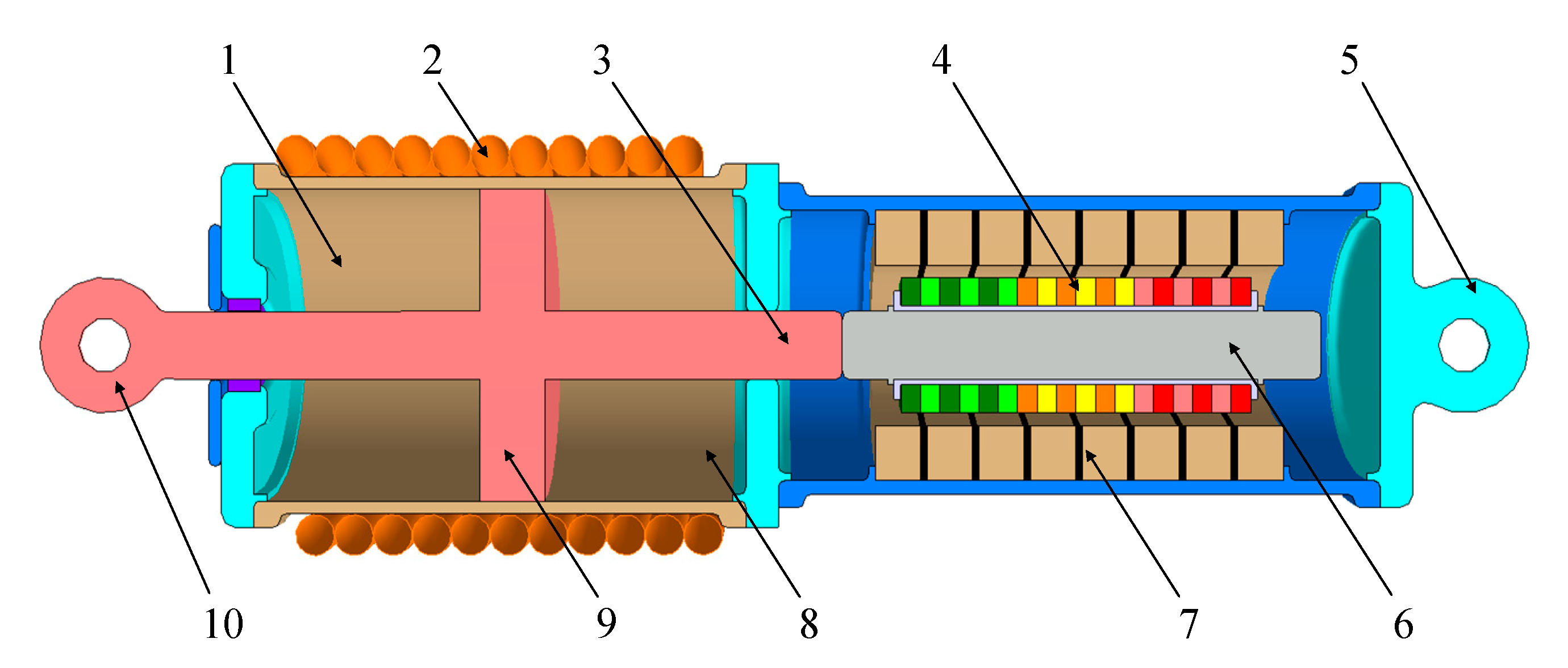
2. Basic Structure and Working Principle of Electromagnetic Inerter

The electromagnetic inerter is composed of a fluid inerter and a linear generator, as shown in Figure 1. The moving rod of the linear generator is interconnected with the piston rod of the fluid inerter. The coil of the linear generator is connected with an external electrical circuit.

For a fluid inerter, when relative displacement of the two terminals of this device occurs, the piston pushes the fluid through the helical tube. This process is similar to the conversion of linear motion to rotational motion in a rack and pinion inerter and ball–screw inerter. In this procedure, the fluid flows through the helical tube, forming the mechanical properties of the inerter.

According to the conservation of hydraulic cylinder volume, the following equations can be obtained:

$$S_1=\pi (r_2^2-r_1^2)$$

(1)

$$S_2=\pi r_3^2$$

(2)

$$S_{1}x=\frac{\theta }{2\pi }{S}_2\sqrt{h^2+{\left(2\pi r_4\right)}^2}$$

(3)

x represents the displacement of the piston and θ represents the Angle at which a piece of fluid media rotates in the helical tube. S₁ and S₂ are the cross-sectional area of the hydraulic cylinder and the cross-sectional area of the helical tube, respectively. The four parameters r₁, r₂, r₃, and r₄ are, respectively: the radius of the piston rod, the radius of the hydraulic cylinder, the inner radius of the helical tube, and the rotation radius of the helical tube. h is the lead of the helical tube.

According to the law of energy conservation, the following equations can be obtained:

$$J=m{r}_4^2$$

(4)

$$l=\sqrt{h^2+{(2\pi r_4)}^2}\times n$$

(5)

$$m=\rho S_{2}l$$

(6)

$$\frac{1}{2}b{(\frac{dx}{dt})}^2=\frac{1}{2}J{(\frac{d\theta }{dt})}^2$$

(7)

J is the moment of inertia when the fluid flows, m is the mass of the fluid that is in the helical tube, n is the number of turns of the helical tube, ρ is the density of the fluid, l is the length of the helical tube, and b is the inertance coefficient.

Therefore, the mechanical inertance coefficient b in the EMI can be expressed as follows:

$$b=\frac{m}{1+{\left(\frac{h}{2\pi r_4}\right)}^2}{\left(\frac{S_1}{S_2}\right)}^2$$

(8)

The derivation process of the above equations follows the same basic principle as [41]. At the same time, it can be easily known from the above equations that a different inertance coefficient b can be obtained by adjusting the cross-sectional area of the hydraulic cylinder, the cross-sectional area of the helical tube, the helical tube rotation radius, the helical tube pitch, and other parameters.

For the part of linear generator, the electromotance U_g is generated when the moving rod shifts relative to the stator. The value of electromotance is proportional to the velocity of relative motion, which conforms to the following equation:

$$U_g=k_e{v}_a$$

(9)

where k_e is the voltage coefficient and v_a is the relative motion velocity of the moving rod and stator.

The relationship between the thrust F_e of the linear generator and current I_a conforms to the following equation:

$$F_e=k_t{I}_a$$

(10)

k_t is the force coefficient and I_a is the current through the stator.

Under ideal conditions, and considering the existence of an external circuit for which the impedance is Z_e(s) at the external port, the relationship between the current and voltage of the linear generator is as follows:

$$\frac{I_a\left(s\right)}{U_g\left(s\right)}=\frac{1}{Z_e\left(s\right)}$$

(11)

The stator of linear generator itself contains inductance and resistance. If the influence of these nonlinear factors is considered, the expression should be corrected as follows:

$$\frac{I_a\left(s\right)}{U_g\left(s\right)}=\frac{1}{R_e+s{L}_e+Z_e\left(s\right)}$$

(12)

where I_a(s) and U_g(s) are the Laplacian forms of current and voltage and R_e and L_e are the resistance and inductance of the windings, respectively.

Based on Equations (8)–(11), the velocity impedance of this device can be obtained:

$$\frac{F\left(s\right)}{v\left(s\right)}=\frac{m}{1+{\left(\frac{\mathrm{h}}{2\pi {\mathrm{r}}_4}\right)}^2}{\left(\frac{S_1}{S_2}\right)}^{2}s+\frac{k_e{k}_t}{Z_e\left(s\right)}$$

(13)

If the effect of internal resistance and inductance of the linear generator is considered, the expression becomes the following:

$$\frac{F\left(s\right)}{v\left(s\right)}=\frac{m}{1+{\left(\frac{\mathrm{h}}{2\pi {\mathrm{r}}_4}\right)}^2}{\left(\frac{S_1}{S_2}\right)}^{2}s+\frac{k_e{k}_t}{R_e+s{L}_e+Z_e\left(s\right)}$$

(14)

It should be pointed out that the above equation is only an ideal model of an EMI, which ignores the mass of the moving parts themselves and the friction between the seal and the cylinder wall or the piston rod; the viscosity of the fluid and the gas, which may not drain, are also not taken into account.

To better illustrate how the device works, a block diagram is presented in Figure 2. The red dotted line inside represents the linear generator and its external circuit in this device; the force of their output is F_e(t). F_bm(t) is the inertance force generated by the fluid in the helical tube.

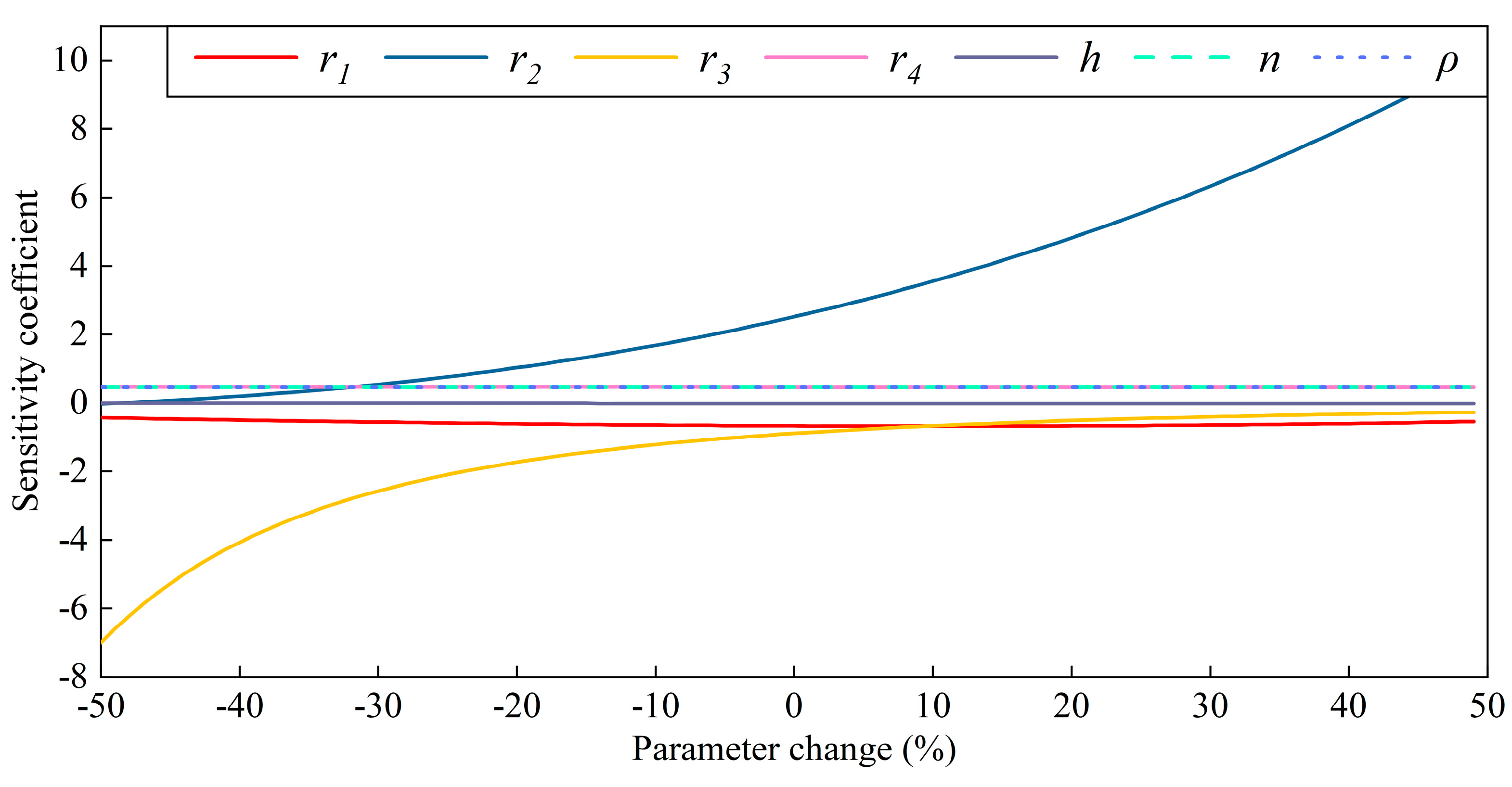
3. Parametric Sensitivity Analysis of Fluid Inerter

Seven parameters determine the inertance coefficient value in the fluid inerter, including six geometric dimensions and fluid density. For sensitivity analysis, it is conducted on the parameters r₁, r₂, r₃, r₄, h, n, and ρ, and the central values of these seven parameters are set at 13 mm, 25 mm, 6 mm, 40 mm, 40 mm, 10 turns, and 1000 kg/m³. The sensitivity coefficient is used as the evaluation indicator of the sensitivity level of parameters, and it is calculated by Equation (15). S and p are the sensitivity coefficient and the percentage of the parameter change, respectively.

$$S=db/dp$$

(15)

As shown in Figure 3, two extremely distinct curves, r₂ and r₃, appear a completely different shape from the other lines. It can be considered that the inertance coefficient of the device is sensitive to these two parameters and that adjustment of these two parameters should be given priority when the inertance coefficient needs to be substantially increased or decreased. When the inertance coefficient needs to be adjusted slightly, r₁, r₄, and n can be adjusted for a more accurate device. It should be noted that the parameter h has almost no effect on the inertance coefficient.

In addition, the density of the fluid, which is usually determined by other properties of the fluid itself, has a linear effect on the inertance coefficient. In the actual use process, objective factors such as temperature and pressure have little influence on its density, and the influence on the inertance coefficient can be almost negligible.

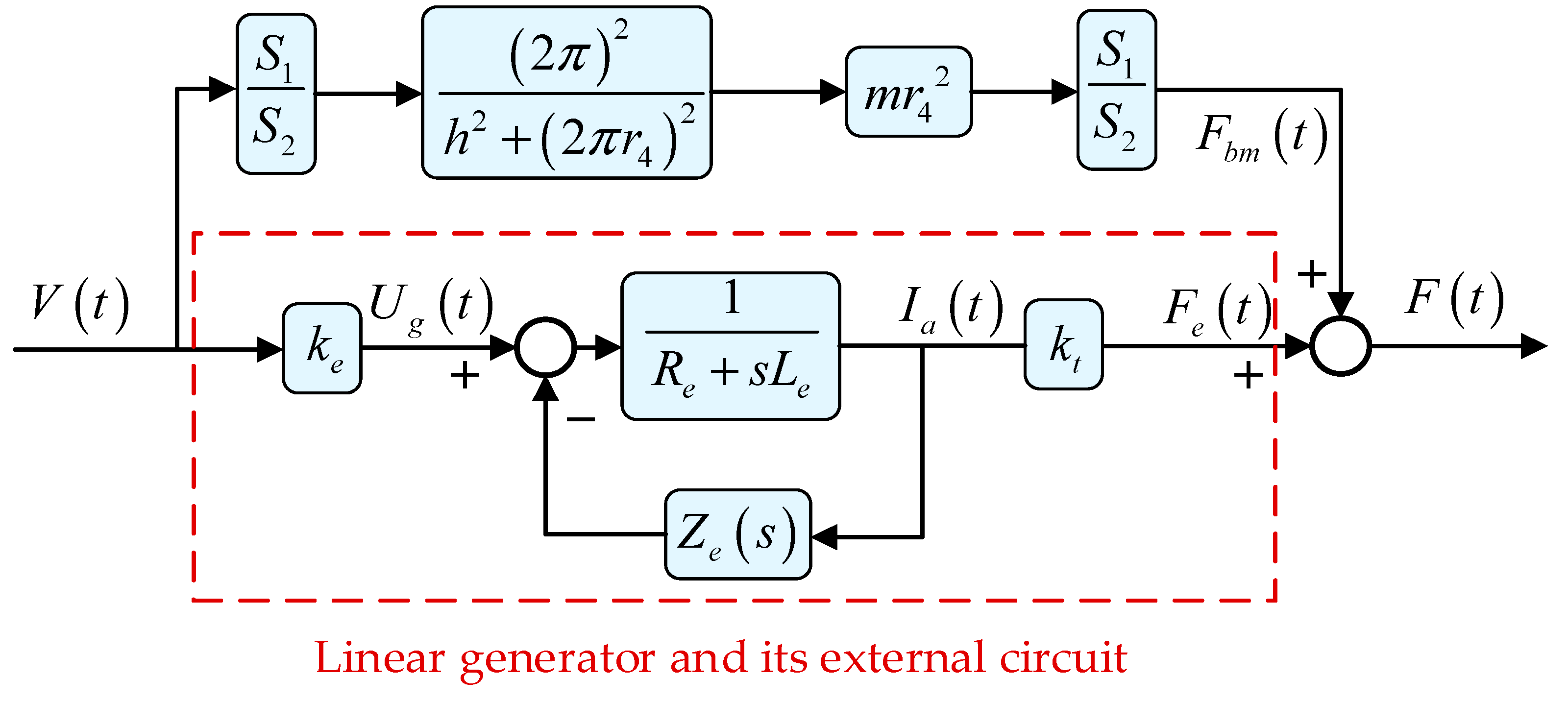
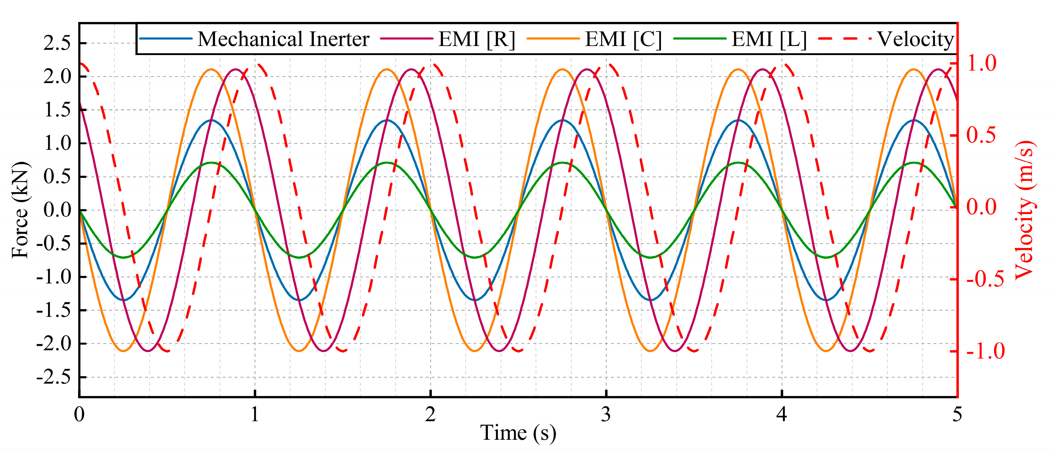
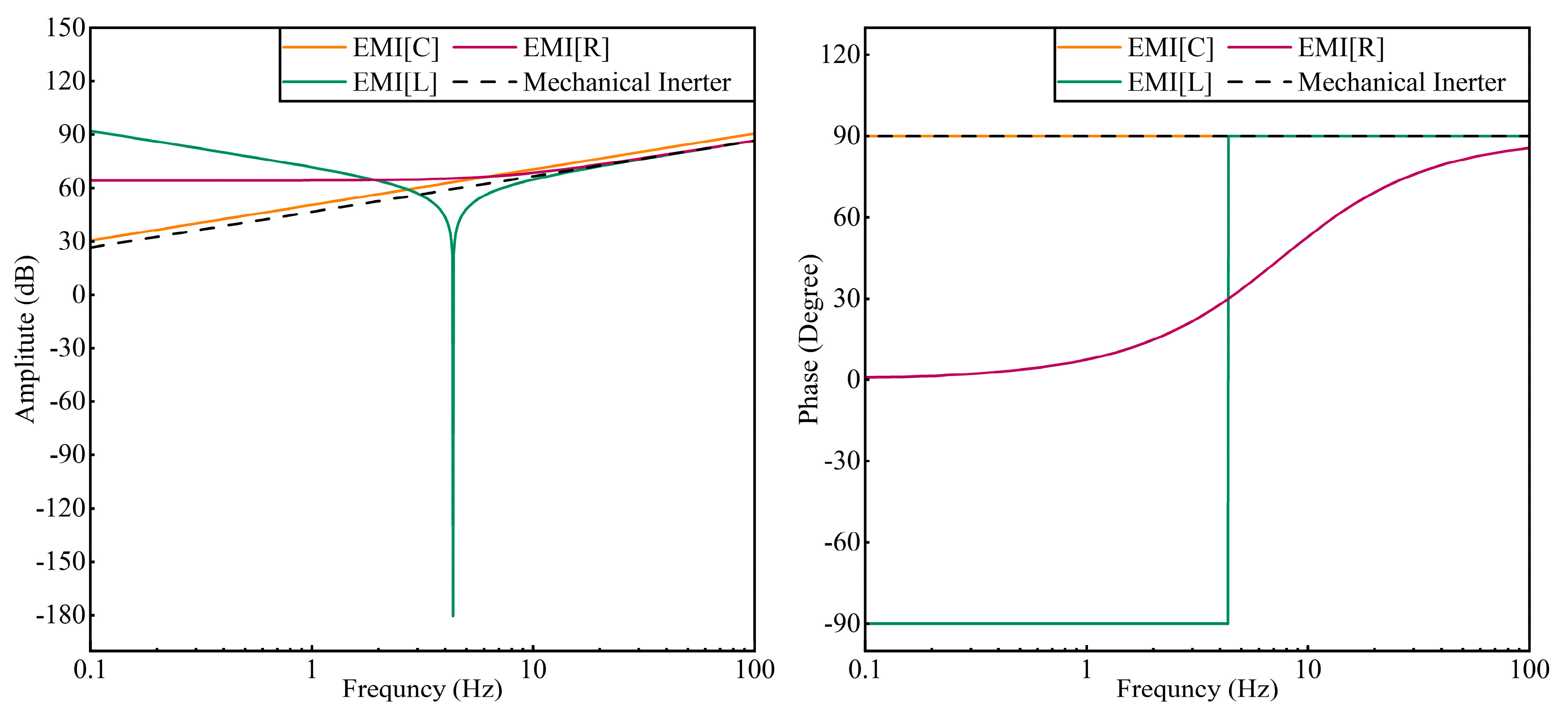
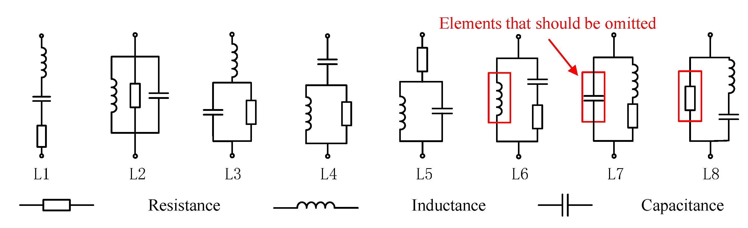
4. The Influence of External Circuits on the Output Characteristics of the Device

The function of the external circuit on the device should conform to the electrical—mechanical analogies. In order to verify this theory, the resistor, inductor, and capacitor are connected to the external port of the linear generator, respectively. Their effect on the device shall, respectively, be equivalent to the parallel damping, spring, and inerter on the basis of the fluid inerter. The relevant parameters are listed in

Table 1. The parameters used to determine the influence of external circuits.

Parameter	Symbol	Unit	Value
Inner radius of the hydraulic cylinder	r1	m	0.04
Radius of the piston rod	r2	m	0.0125
Inner radius of helix tube	r3	m	0.0085
The radius of rotation of helix tube	r4	m	0.078
Lead of the helix tube	h	m	0.0095
The number of turns of the helical tube	n	-	7
Fluid density	ρ	kg/m3	690
Voltage coefficient	Ke	V/(m/s)	100
Force coefficient	Kt	N/A	81
Resistance of the external circuit (resistance only)	R	Ω	5
Capacitance size of external circuit (capacitance only)	C	F	0.015
Inductance size of external circuit (inductance only)	L	H	2

.

The spring and inerter will produce a 90° phase lag and 90° phase advance, respectively, after receiving sinusoidal velocity excitation, and for damping, it is consistent with the phase of the velocity. Similarly, according to the electrical–mechanical analogies, the phase of the inductors and capacitors will be 90° behind or the ahead sinusoidal excitation current, respectively, and the phase of the resistors is the same as that of the current.

Figure 4 illustrates the output characteristic of the EMI device when the external circuit is changing. EMI[R], EMI[C], and EMI[L], respectively, represent connecting a resistor, capacitor, or inductor to the external circuit. This verifies the above rules about the phase of the output. The blue curve represents the output force of the mechanical part in the time domain, which is the output curve of the fluid inerter in the EMI, and the orange, wine, and green curves reveal the output characteristics of the entire device. The wine curve clearly shows that the mechanical part and the electrical part of the EMI are superimposed, and connecting resistors to the linear generator is actually equivalent to connecting a damper in parallel to the EMI device. The phase difference in the EMI (the outside circuit only contains a resistor) is between the phase of the velocity excitation and the output phase of the mechanical inertance element, because the inertance element and the damping element have the characteristics of phase advance and phase invariance, respectively. Similarly, the green and orange curves show the output curves of inductance and capacitance connected externally to the linear generator. Since the corresponding mechanical components of inductance and capacitance are the spring and inerter, respectively, it can actually be regarded as the fluid inerter in parallel with the components equivalent to the spring and inerter in the electrical network. It is precisely because of the similarity between electrical and mechanical components that the device has the ability to achieve a complex impedance transfer function through a simple mechanical structure.

In Figure 5, the Bode diagram of the EMI connected with capacitor, resistor, and inductor is drawn and compared with the amplitude–frequency characteristics of the mechanical inerter. From the perspective of frequency domain, the EMI device also addresses the same characteristic as shown in time domain. This also verifies the conclusions obtained in the above time domain analysis, such as the phase advance characteristic of the inerter; the external inductance is equivalent to a parallel spring and presents the characteristic of phase lag, and the external capacitor presents the characteristic of the partial superposition of the inertance coefficient, etc. In addition, between 4 and 5 Hz, when the external circuit is the inductor, the output characteristics of the device will change greatly. There will be a large reduction in the output amplitude of the device, and the phase will change from a 90° phase lag to a 90° phase advance. Beyond this frequency range, the inertance part of the device will output a force greater than that of the spring (equivalent to the inductor).

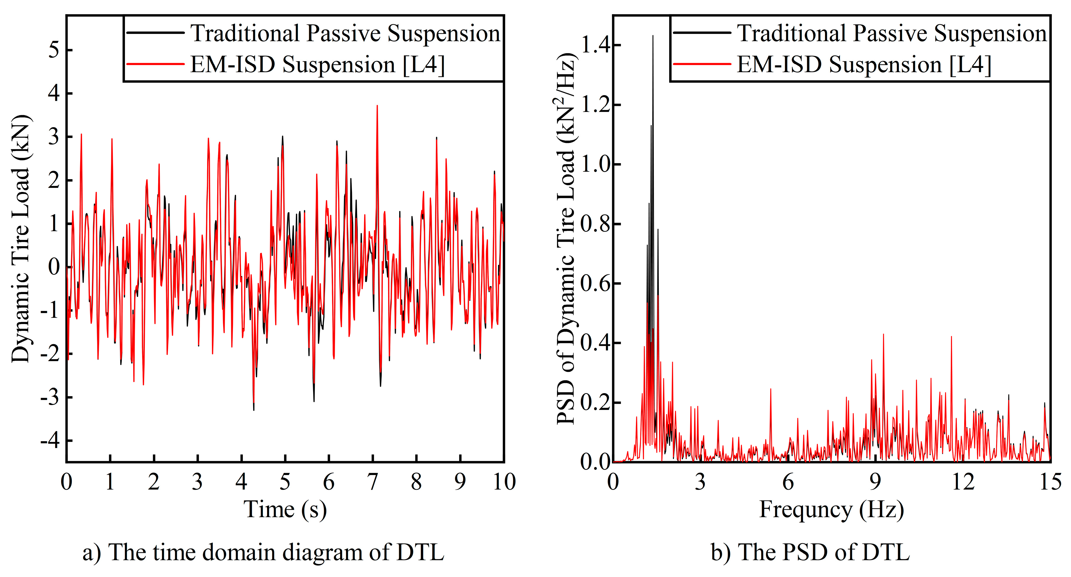
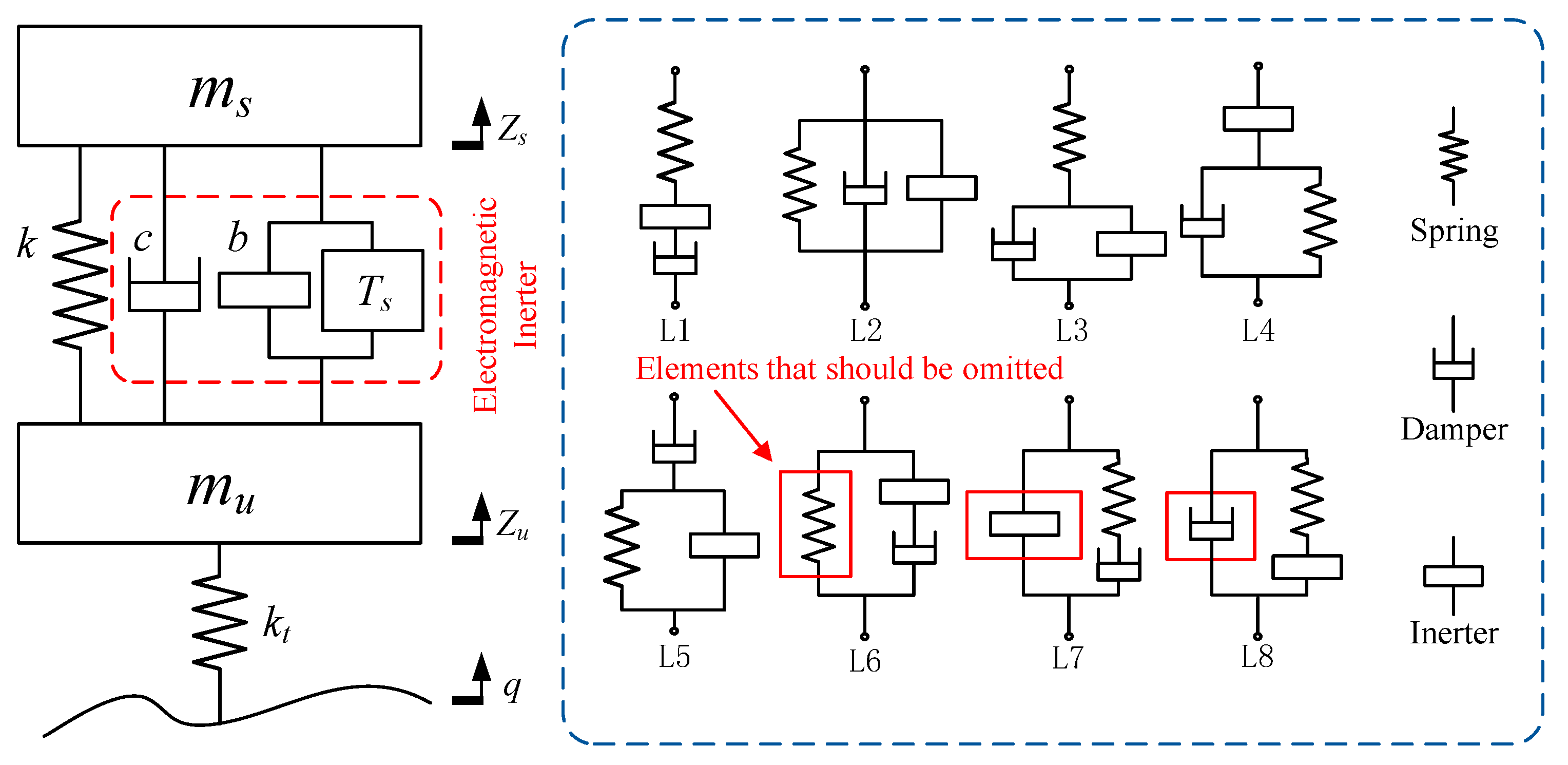
5. Quarter Vehicle Model with Electromagnetic Inerter–Spring–Damper (EM-ISD) Suspension System

In order to prove that the introduction of a mechatronics structure in a suspension system is advantageous, a widely used quarter vehicle model is adopted in this paper. The layouts of this suspension system are shown in Figure 6. The red dotted box represents the mechatronics structure used to replace the damper in the passive suspension, where b is the mechanical inertance component of the structure, c is the damping component, and T_s represents the impedance of the linear generator and external circuit. The eight layouts, from L1 to L8, in the blue dotted box can be realized by the linear generator and the external circuit; the specific structure of the external circuit is shown in Figure 7. The important thing to notice here is that the layout of L2 shown in Figure 6 and Figure 7 is essentially a superposition of spring, damper, and inerter. Therefore, this layout will be degraded to a three-parallel structure (spring, damper, and inerter) in practice. If the structure is analyzed according to the optimization objectives as described below, it will directly degenerate into traditional passive suspension, so this structure will not be discussed. Meanwhile, L6, L7, and L8 also have duplicate components; the duplicates in these structures (in the solid red boxes of Figure 6 and Figure 7) should be removed.

$$\left\{\begin{array}{l}{m}_s{\ddot{z}}_s+k\left(z_s-z_u\right)+c\left({\dot{z}}_s-{\dot{z}}_u\right)+b\left({\ddot{z}}_s-{\ddot{z}}_u\right)+T_s\left({\dot{z}}_s-{\dot{z}}_u\right)=0\hfill \\ m_u{\ddot{z}}_u-k\left(z_s-z_u\right)-c\left({\dot{z}}_s-{\dot{z}}_u\right)-b\left({\ddot{z}}_s-{\ddot{z}}_u\right)-T_s\left({\dot{z}}_s-{\dot{z}}_u\right)+k_t\left(z_u-q\right)=0\hfill \end{array}\right.$$

(16)

The dynamic equations are presented in Equation (16), where m_s and m_u are sprung mass and unsprung mass, respectively. z_s and z_u represent the displacement of the sprung mass and unsprung mass. k and k_t are the main spring stiffness and tire equivalent stiffness. q is the random road excitation. T_s is the velocity-type impedance expression of the EMI. The analytical expression of random road excitation is as follows:

$$\dot{q}\left(t\right)=-2\pi f_{0}q\left(t\right)+2\pi \sqrt{G_{0}v}w\left(t\right)$$

(17)

where G₀ is the road roughness coefficient, v is the vehicle velocity, f₀ is the lower cut-off frequency, and w(t) is the Gaussian white noise, for which the mean value is 0 [42].

To acquire the most appropriate parameters for each structure in this case, an optimized method named “Harris hawks optimization (HHO)” is adopted. As a type of metaheuristic algorithm, this optimizer simulates the hunting behavior of Harris hawks that forage with other members of their family. Compared with the genetic algorithm (GA), particle swarm optimization (PSO), grey wolf optimization (GWO), etc., HHO has significant advantages in dealing with multi-dimensional problems. In addition, as an optimization algorithm with a variety of exploratory and exploitative mechanisms, HHO has a higher potential in jumping out of the local optimal solution. The literature [43] shows a more specific introduction and related research on this optimization algorithm.

For the optimization process of a certain system, the optimization objective and optimization parameters should be clarified first. Since the main spring has a load-bearing function, it is not considered as one of the optimization parameters. The optimization parameters include inertance b, resistance R, inductance L, and capacitance C. The specific values of other suspension parameters are shown in

Table 2. The basic parameters of the quarter model.

Parameter [Unit]	Value
Suspension spring stiffness k [N/m]	35,000
Tire equivalent stiffness kt [N/m]	190,000
Sprung mass ms [kg]	400
Unsprung mass mu [kg]	45
Damping coefficient of EM-ISD suspension c [N/(m/s)]	300–2700 (step size: 50)

.

The root mean square (RMS) values of body acceleration (BA), suspension working space (SWS), and dynamic tire load (DTL) are three indicators used to evaluate the vibration isolation ability of the suspension system. For convenience, these three parameters are simply denoted as RMS(BA), RMS(SWS), and RMS(DTL). Using these three indicators as an optimization objective is a commonly used approach. A more detailed description of this optimization method can be found in Reference [42]. However, RMS(SWS) is relatively unique among these three indicators; the main reason to limit this value is to reduce the probability of the suspension hitting the buffer block. Therefore, it may be an option to restrict the maximum SWS value directly to a certain range. The other two performance indicators, RMS(BA) and RMS(DTL), are related to passenger comfort and handling stability, respectively, and excessive RMS(DTL) may cause damage to the road [44]. On this basis, RMS(BA) is taken as the most important optimization objective Obj, and RMS(DTL) is guaranteed to not be inferior to traditional passive suspension. Finally, the final optimization objective is shown in Equation (18). Under this condition, the HHO algorithm will try to obtain the best passenger comfort and handling stability, superior to that of traditional passive suspension.

$$\left\{\begin{array}{l}\mathit{O}\mathit{b}\mathit{j}=\mathrm{RMS}\left({\mathrm{BA}}_{\mathrm{EM}-\mathrm{ISD}}\right);\\ \mathrm{RMS}\left({\mathrm{DTL}}_{\mathrm{EM}-\mathrm{ISD}}\right)<\mathrm{RMS}\left({\mathrm{DTL}}_{\mathrm{PA}}\right);\\ \mathrm{MAX}\left[\mathrm{ABS}\left({\mathrm{SWS}}_{\mathrm{EM}-\mathrm{ISD}}\right)\right]<50\mathrm{mm}.\end{array}\right.$$

(18)

RMS(BA_EM-ISD) represents the RMS(BA) of the EM-ISD suspension. RMS(DTL_EM-ISD) and RMS(DTL_PA) represent the RMS(DTL) of EM-ISD suspension and traditional passive suspension, respectively. Max[ABS(SWS_EM-ISD)] represents the maximum operating range of the suspension.

Before discussing Figure 8, the minimal value of RMS(BA_PA) and RMS(DTL_PA) are defined as the reference value first. To describe the performance change, the following equation is defined:

$$P_i=\left|1-\frac{\mathrm{RMS}(i)}{\mathrm{MIN}[\mathrm{RMS}(i_{\mathrm{PA}})]}\right|\times 100\%$$

(19)

In the above equation, if the performance indicator discussed is related to body acceleration, then i is “BA”; if it is related to tire dynamic load, then i is “DTL”.

According to Figure 8, the following points can be found:

1. When the damping coefficient is about 1850 N/(m/s), the RMS(BA_PA) reaches the lowest value, and the passenger comfort performance parameter is maximized, but the RMS(DTL_PA) reaches 1109 N. Only when the damping coefficient is about 2650 N/(m/s) does the RMS(DTL_PA) reach the lowest value (1071 N), and RMS(BA_PA) rises to 2.092 m/s².

2. When the RMS(BA_EM-ISD) of L1, L3, and L4 reaches MIN[RMS(BA_PA)], the damper coefficient is near 2300 N/(m/s), and the RMS(DTL_EM-ISD) is 0.54% larger than MIN[RMS(DTL_PA)]. This is far less than the performance degradation (3.52%) of the RMS(DTL_PA) at a damping coefficient of 1850 N/(m/s).

3. Setting the damping coefficient as 1850 N(m/s), at this point, RMS (BA_PA) is at the lowest value. Under this value, the RMS(BA_EM-ISD) of L1, L3, L4, L5, L6, L7, and L8 promote 4.52%, 3.66%, 4.56%, 1.46%, 1.02%, 1.26%, and 0.65%, respectively.

4. When the damping coefficient is greater than 1500 N/(m/s), there is almost no difference in the RMS_TDL of different layouts due to the limitation of the optimization boundary, while the RMS_BA of L1 and L4 are the same and better than other layouts. When the damping coefficient is less than 1500 N/(m/s), with the decreases in damping coefficient, L4, L6, and L8 seem to plateau when the RMS_TDL rises, which makes the rise in the RMS_TDL of these three layouts limited and not as dramatic as for L1, L3, L5, and L7. For L6 and L8, no matter how relaxed the RMS_TDL is, their RMS_BA could not be reduced to 1.9263 m/s2. However, layout L4 can reduce the RMS_BA to this value when the parallel damping is 1850 N/(m/s) and the RMS_TDL is only 1109 N. Therefore, the potential of L6 and L8 is very limited from the perspective of relaxing the requirements of RMS_DTL to improve occupant comfort.

On the basis of the above points, the following conclusions can be drawn:

1. From the first and second points above, it can be found that in traditional passive suspension, it is difficult to coordinate the RMS(BA_PA) and the RMS(DTL_PA) at the same time, and both of them cannot reach the minimum value simultaneously. However, the dynamic performance of suspension is changed, and the dynamic performance boundary of the vibration isolation system is expanded after the EM-ISD suspension is adopted. Especially when the layouts L1, L3, and L4 are employed, the lowest RMS(BA_PA) and the lowest RMS(DTL_PA) can be reached almost simultaneously.

2. From the perspective of the third and fifth points above, the L4 layout should be considered as the optimal suspension structure. Compared with traditional passive suspension, better passenger comfort performance can be obtained under the same conditions, and it ensures that the RMS (DTL_EM-ISD) is not higher than that of traditional passive suspension.

To further verify the vibration isolation capability, the dynamic performance of layout L4 was analyzed when the damping coefficient is 1850 N/(m/s), and compared with traditional passive suspension. The optimal parameters obtained after optimization are shown in

Table 3. The optimized suspension parameters of L4.

Parameter [Unit]	Value
Inertance coefficient [kg]	6.8
Inductance [H]	1.8
Capacitance [mF]	7.2
Resistance [Ω]	54
Damping coefficient [N/(m/s)]	1850

.

In Figure 9, Figure 10 and Figure 11 the response characteristics of BA, DTL, and SWS under random road excitation are presented. From the perspective of time domain, the range of change in SWS of L4 is significantly lower than that of traditional passive suspension. For BA, the value also decreased slightly after L4 was used. There is not a distinct difference between the DTL of L4 and traditional passive suspension. The power spectral density (PSD) of BA, DTL, and SWS is obtained by the fast Fourier transform (FFT) of the result in the time domain. Whether BA, DTL, or SWS, the power spectral density of L4 near the frequency of 1.4 Hz is smaller than that of traditional passive suspension. This demonstrates that L4 has the ability to suppress vehicle vibration at the offset frequency.

Table 4. Comparison of main performance indicators between EM-ISD suspension and traditional passive suspension.

Structure	RMS(BA) [m/s2]	RMS(DTL) [N]	RMS(SWS) [mm]	MAX(SWS) [mm]
Traditional passive suspension	2.016359	1097.28	15.828	0.048
EM-ISD suspension (L4)	1.921581	1097.16	13.644	0.043

compares the main performance indicators of EM-ISD suspension and traditional passive suspension. Similar to the time domain diagram, L4 showed varying degrees of performance improvement on SWS and BA, but DTL was basically consistent with traditional passive suspension.

6. Conclusions

A new type of inerter based on a linear generator and a fluid inerter is researched in this paper. Firstly, the structure and working principle of this device are introduced. Then, a dynamic model is established by analyzing the working process of the device, and the implementability of the simulated mechanical network is verified. It is proved that complex mechanical topologies can be simplified by introducing external circuits. On this basis, the influence of geometric dimension parameters on the inertance coefficient of the fluid domain is analyzed, and two parameters sensitive to the inertance coefficient are obtained. Finally, a quarter suspension model is established to study the effect of the device on the dynamic performance of the suspension. Furthermore, the performance advantages are analyzed from the perspective of time and frequency domains. The results show that vehicle suspension using the EMI has better vibration isolation performance than traditional passive suspension.

Future research on this device will focus on two directions: one is how to use more accurate simulation means to study the difficulties of the device in practical engineering applications [45], and the other is to combine it with the whole vehicle to discuss its coupling and matching relationship in the comprehensive dynamic performance of the vehicle [46].

References

1. Smith, M.C. Synthesis of Mechanical Networks: The Inerter. IEEE Trans. Autom. Control. 2002, 47, 1648–1662. [Google Scholar] [CrossRef]
2. Chang, Y.; Zhou, J.; Wang, K.; Xu, D. A Quasi-Zero-Stiffness Dynamic Vibration Absorber. J. Sound Vib. 2021, 494, 115859. [Google Scholar] [CrossRef]
3. Qin, Y.; Zhao, Z.; Wang, Z.; Li, G. Study of Longitudinal–Vertical Dynamics for In-Wheel Motor-Driven Electric Vehicles. Automot. Innov. 2021, 4, 227–237. [Google Scholar] [CrossRef]
4. Liu, C.; Chen, L.; Lee, H.P.; Yang, Y.; Zhang, X. A Review of the Inerter and Inerter-Based Vibration Isolation: Theory, Devices, and Applications. J. Frankl. Inst. 2022, 359, 7677–7707. [Google Scholar] [CrossRef]
5. De Domenico, D.; Ricciardi, G.; Zhang, R. Optimal Design and Seismic Performance of Tuned Fluid Inerter Applied to Structures with Friction Pendulum Isolators. Soil Dyn. Earthq. Eng. 2020, 132, 106099. [Google Scholar] [CrossRef]
6. Giaralis, A.; Petrini, F. Wind-Induced Vibration Mitigation in Tall Buildings Using the Tuned Mass-Damper-Inerter. J. Struct. Eng. 2017, 143, 04017127. [Google Scholar] [CrossRef]
7. Li, J.; Zhu, S. Cable vibration mitigation by using an H-bridge-based electromagnetic inerter damper with energy harvesting function. Struct. Control Health Monit. 2022, 29, e3120. [Google Scholar] [CrossRef]
8. Sun, L.; Hong, D.; Chen, L. Cables Interconnected with Tuned Inerter Damper for Vibration Mitigation. Eng. Struct. 2017, 151, 57–67. [Google Scholar] [CrossRef]
9. Wang, Q.; Zheng, Z.; Qiao, H.; De Domenico, D. Seismic Protection of Reinforced Concrete Continuous Girder Bridges with In-erter-Based Vibration Absorbers. Soil Dyn. Earthq. Eng. 2023, 164, 107526. [Google Scholar] [CrossRef]
10. Luo, J.; Macdonald, J.H.G.; Jiang, J.Z. Identification of Optimum Cable Vibration Absorbers Using Fixed-Sized-Inerter Layouts. Mech. Mach. Theory 2019, 140, 292–304. [Google Scholar] [CrossRef]
11. Chen, H.; Su, W.; Wang, F. Modeling and Analyses of a Connected Multi-Car Train System Employing the Inerter. Adv. Mech. Eng. 2017, 9, 168781401770170. [Google Scholar] [CrossRef]
12. Wang, F.; Liao, M.; Liao, B.; Su, W.; Chan, H.A. The Performance Improvements of Train Suspension Systems with Mechanical Networks Employing Inerters. Veh. Syst. Dyn. 2009, 47, 805–830. [Google Scholar] [CrossRef]
13. He, H.; Li, Y.; Jiang, J.Z.; Burrow, S.; Neild, S.; Conn, A. Using an Inerter to Enhance an Active-Passive-Combined Vehicle Suspension System. Int. J. Mech. Sci. 2021, 204, 106535. [Google Scholar] [CrossRef]
14. Shen, Y.; Jia, M.; Yang, X.; Liu, Y.; Chen, L. Vibration Suppression Using a Mechatronic PDD-ISD-Combined Vehicle Suspension System. Int. J. Mech. Sci. 2023, 250, 108277. [Google Scholar] [CrossRef]
15. Shen, Y.; Chen, A.; Du, F.; Yang, X.; Liu, Y.; Chen, L. Optimal design and dynamic performance analysis of semi-active vehicle air ISD suspension. Proc. Inst. Mech. Eng. Part D J. Automob. Eng. 2024. [Google Scholar] [CrossRef]
16. Hu, Y.; Wang, J.; Chen, M.Z.Q.; Li, Z.; Sun, Y. Load Mitigation for a Barge-Type Floating Offshore Wind Turbine via Inerter-Based Passive Structural Control. Eng. Struct. 2018, 177, 198–209. [Google Scholar] [CrossRef]
17. Sarkar, S.; Fitzgerald, B. Fluid Inerter for Optimal Vibration Control of Floating Offshore Wind Turbine Towers. Eng. Struct. 2022, 266, 114558. [Google Scholar] [CrossRef]
18. Li, Y.; Jiang, J.Z.; Neild, S. Inerter-Based Configurations for Main-Landing-Gear Shimmy Suppression. J. Aircr. 2017, 54, 684–693. [Google Scholar] [CrossRef]
19. Asai, T.; Sugiura, K. Numerical Evaluation of a Two-Body Point Absorber Wave Energy Converter with a Tuned Inerter. Renew. Energy 2021, 171, 217–226. [Google Scholar] [CrossRef]
20. Nemoto, Y.; Takino, M.; Tsukamoto, S.; Asai, T. Numerical Study of a Point Absorber Wave Energy Converter with Tuned Variable Inerter. Ocean. Eng. 2022, 257, 111696. [Google Scholar] [CrossRef]
21. Papageorgiou, C.; Houghton, N.E.; Smith, M.C. Experimental Testing and Analysis of Inerter Devices. J. Dyn. Syst. Meas. Control 2009, 131, 011001. [Google Scholar] [CrossRef]
22. Siami, A.; Karimi, H.R. Modelling and Identification of the Hysteretic Dynamics of Inerters. Designs 2020, 4, 27. [Google Scholar] [CrossRef]
23. Wang, F.; Hong, M.; Lin, T. Designing and Testing a Hydraulic Inerter. Proc. Inst. Mech. Eng. Part C J. Mech. Eng. Sci. 2011, 225, 66–72. [Google Scholar] [CrossRef]
24. Swift, S.J.; Smith, M.C.; Glover, A.R.; Papageorgiou, C.; Gartner, B.; Houghton, N.E. Design and Modelling of a Fluid Inerter. Int. J. Control 2013, 86, 2035–2051. [Google Scholar] [CrossRef]
25. Ge, Z.; Wang, W. Modeling, Testing, and Characteristic Analysis of a Planetary Flywheel Inerter. Shock Vib. 2018, 2018, 2631539. [Google Scholar] [CrossRef]
26. John, E.D.A.; Wagg, D.J. Design and Testing of a Frictionless Mechanical Inerter Device Using Living-Hinges. J. Frankl. Inst. 2019, 356, 7650–7668. [Google Scholar] [CrossRef]
27. Málaga Chuquitaype, C.; Menendez Vicente, C.; Thiers Moggia, R. Experimental and Numerical Assessment of the Seismic Response of Steel Structures with Clutched Inerters. Soil Dyn. Earthq. Eng. 2019, 121, 200–211. [Google Scholar] [CrossRef]
28. Lazarek, M.; Brzeski, P.; Perlikowski, P. Design and Identification of Parameters of Tuned Mass Damper with Inerter Which Enables Changes of Inertance. Mech. Mach. Theory 2018, 119, 161–173. [Google Scholar] [CrossRef]
29. Li, Y.; Cheng, Z.; Hu, N.; Yang, Y.; Yin, Z. Study of Dynamic Breakdown of Inerter and the Improved Design. Mech. Syst. Signal Process. 2022, 167, 108520. [Google Scholar] [CrossRef]
30. Chillemi, M.; Furtmüller, T.; Adam, C.; Pirrotta, A. Nonlinear Mechanical Model of a Fluid Inerter. Mech. Syst. Signal Process. 2023, 188, 109986. [Google Scholar] [CrossRef]
31. Liu, X.; Jiang, J.Z.; Titurus, B.; Harrison, A. Model Identification Methodology for Fluid-Based Inerters. Mech. Syst. Signal Process. 2018, 106, 479–494. [Google Scholar] [CrossRef]
32. Liu, X.; Titurus, B.; Jiang, J.Z. Generalisable Model Development for Fluid-Inerter Integrated Damping Devices. Mech. Mach. Theory 2019, 137, 1–22. [Google Scholar] [CrossRef]
33. Wang, F.; Chan, H. Vehicle Suspensions with a Mechatronic Network Strut. Veh. Syst. Dyn. 2011, 49, 811–830. [Google Scholar] [CrossRef]
34. Firestone, F.A. A New Analogy Between Mechanical and Electrical Systems. J. Acoust. Soc. Am. 1933, 4, 249–267. [Google Scholar] [CrossRef]
35. Shen, Y.; Shi, D.; Chen, L.; Liu, Y.; Yang, X. Modeling and Experimental Tests of Hydraulic Electric Inerter. Sci. China Technol. Sci. 2019, 62, 2161–2169. [Google Scholar] [CrossRef]
36. Zuo, L.; Scully, B.; Shestani, J.; Zhou, Y. Design and Characterization of an Electromagnetic Energy Harvester for Vehicle Suspensions. Smart Mater. Struct. 2010, 19, 045003. [Google Scholar] [CrossRef]
37. Rhinefrank, K.; Schacher, A.; Prudell, J.; Brekken, T.K.A.; Stillinger, C.; Yen, J.Z.; Ernst, S.G.; von Jouanne, A.; Amon, E.; Paasch, R.; et al. Comparison of Direct-Drive Power Takeoff Systems for Ocean Wave Energy Applications. IEEE J. Ocean. Eng. 2012, 37, 35–44. [Google Scholar] [CrossRef]
38. Orkisz, P.; Sapiński, B. Vibration Reduction System with a Linear Motor: Operation Modes, Dynamic Performance, Energy Consumption. Energies 2022, 15, 1910. [Google Scholar] [CrossRef]
39. Wen, X.; Li, Y.; Yang, C. Design, Modeling, and Characterization of a Tubular Linear Vibration Energy Harvester for Integrated Active Wheel System. Automot. Innov. 2021, 4, 413–429. [Google Scholar] [CrossRef]
40. Luo, C.; Yang, X.; Jia, Z.; Liu, C. Layout Optimization and Performance Analysis of Vehicle Suspension System Using an Electromagnetic Inerter. World Electr. Veh. J. 2023, 14, 318. [Google Scholar] [CrossRef]
41. Glover, A.R.; Smith, M.C.; Houghton, N.E.; Long, P.J.G. Force-Controlling Hydraulic Device. UK. Patent GB0913759D0, 6 August 2009. [Google Scholar]
42. Shen, Y.; Hua, J.; Fan, W.; Liu, Y.; Yang, X.; Chen, L. Optimal Design and Dynamic Performance Analysis of a Fractional-Order Electrical Network-Based Vehicle Mechatronic ISD Suspension. Mech. Syst. Signal Process. 2023, 184, 109718. [Google Scholar] [CrossRef]
43. Heidari, A.A.; Mirjalili, S.; Faris, H.; Aljarah, I.; Mafarja, M.; Chen, H. Harris Hawks Optimization: Algorithm and Applications. Future Gener. Comput. Syst. 2019, 97, 849–872. [Google Scholar] [CrossRef]
44. Liu, D.; Jiang, R.; Yang, Y.; Wang, S. Simulation Study of Heavy Vehicle Road-Friendliness under Bilateral Tracks’ Excitation. Adv. Mater. Res. 2013, 680, 422–428. [Google Scholar] [CrossRef]
45. Chillemi, M. Experimental and Numerical Investigation of a Fluid Inerter for Structural Control. J. Sound Vib. 2024, 573, 118222. [Google Scholar] [CrossRef]
46. Wiseman, Y. Efficient Embedded Computing Component for Anti-Lock Braking System. Int. J. Control. Autom. 2018, 11, 1–10. [Google Scholar]
Figure 1. The basic structure of an EMI: 1 and 8 are the chamber of the hydraulic cylinder; 2 is the helical tube; 3 is the piston rod of the main cylinder; 4 is the moving magnetic pole; 5 and 10 are the two terminals of the EMI—they should be connected to the body and wheels in the vehicle’s suspension; 6 is the moving rod of the linear generator; 7 is the stator of the linear generator; 9 is the piston.
Wevj 15 00162 g001
Figure 2. Block diagram of EMI.
Wevj 15 00162 g002
Figure 3. Parameter sensitivity analysis of fluid inerter.
Wevj 15 00162 g003
Figure 4. Time domain response curve of the mechanical inerter and the EMI (the external circuit is connected to the capacitor, resistor, and inductor, respectively) under sinusoidal velocity excitation.
Wevj 15 00162 g004
Figure 5. The Bode diagram of the EMI device after changing the external circuit.
Wevj 15 00162 g005
Figure 6. A quarter suspension model of the vehicle.
Wevj 15 00162 g006
Figure 7. Equivalent external circuit of suspension structure.
Wevj 15 00162 g007
Figure 8. The RMS(BA) and RMS(DTL) of each layout change with the damping coefficient.
Wevj 15 00162 g008
Figure 9. The body acceleration of EM-ISD suspension and traditional passive suspension under random road excitation.
Wevj 15 00162 g009
Figure 10. The dynamic tire load of EM-ISD suspension and traditional passive suspension under random road excitation.
Wevj 15 00162 g010
Figure 11. The suspension working space of EM-ISD suspension and traditional passive suspension under random road excitation.
Wevj 15 00162 g011