Research on an Intelligent Vehicle Trajectory Tracking Method Based on Optimal Control Theory

Abstract

This study aims to explore an intelligent vehicle trajectory tracking control method based on optimal control theory. Considering the limitations of existing control strategies in dealing with signal delays and communication lags, a control strategy combining an anthropomorphic forward-looking reference path and longitudinal velocity closure is proposed to improve the accuracy and stability of intelligent vehicle trajectory tracking. Firstly, according to the vehicle dynamic error tracking model, a linear quadratic regulator (LQR) transverse controller is designed based on the optimal control principle, and a feedforward control strategy is added to reduce the system steady-state error. Secondly, an anthropomorphic look-ahead prediction model is established to mimic human driving behavior to compensate for the signal lag. The double proportional–integral–derivative (DPID) control algorithm is used to track the longitudinal speed reference value. Finally, a joint simulation is conducted based on MatLab/Simulink2021b and CarSim2019.0 software, and the effectiveness of the control strategy proposed in this paper is verified by constructing a semi-physical experimental platform and carrying out a hardware-in-the-loop test. The simulation and test results show that the control strategy can significantly improve the accuracy and stability of vehicle path tracking, which provides a new idea for future intelligent vehicle control system design.

1. Introduction

With the development of artificial intelligence and control theory, intelligent driving technology has gradually matured, and the intelligent level of transportation systems has been further improved [1]. And the intelligent driving car has made it a worldwide research hotspot due to its great advantages in driving safety and comfort [2]. Intelligent driving technology mainly includes environment sensing and localization, decision making, path planning, and trajectory tracking [3]. Among them, trajectory tracking control is the core of intelligent driving technology, which is an important component to ensure the key performance of vehicle driving safety and maneuvering stability [4].

In recent years, domestic and foreign scholars have also conducted a lot of research on the trajectory tracking of intelligent driving vehicles, such as trajectory tracking control based on optimal control [5], linear quadratic regulator (LQR) [6], proportional–integral–derivative control [7], Stanley modeling [8], model predictive control [9], and other methods. The optimal controller LQR is one of the most popular optimal control theories, which is highly important and representative in modern control theory [10] and has been widely used in a number of fields [11,12]. In 2009, Snider first proposed to utilize the LQR control method for trajectory tracking by using the center of mass of the vehicle as the control point and modeling the system in the presence of path curvature perturbations. In turn, the LQR controller was designed [13]. As described by Xu et al. and Zhang et al., the time delay within the whole vehicle is a major reason for the limitation of trajectory tracking accuracy and instability [14,15]. So, the signal time delay has become a non-negligible issue in the control system for the responsiveness and control accuracy of the vehicle. The signal time delay, either from the sensors and actuators inside the vehicle or from the external communication system, may lead to a lag in the execution of control commands, which in turn affects the tracking performance of the vehicle. To address this problem, numerous studies have proposed various compensation strategies in an attempt to minimize the negative impact of delays. The proportional–integral–derivative (PID) controller is one of the most basic and widely used trajectory tracking algorithms [16]. However, as a linear controller, PID control cannot adapt to complex and variable nonlinear operating conditions [17]. The Stanley controller is considered by many scholars to be a simple, efficient, and proven solution that can provide adequate control performance at low speeds [18]. AbdElmoniem et al. proposed a predictive Stanley lateral control method to calculate steering angle setpoints considering future driving states [19]. However, the Stanley controller is a better solution for applications requiring higher speeds and high dynamics. In the field of trajectory tracking control research, model predictive control (MPC) has also been widely used as a delay compensation method [20]. Yu et al. describe an MPC method that predicts the actual position of the vehicle and uses the delay time as a prediction time to compensate for the effect of delay [21]. While model predictive controllers (MPCs) produce relatively better accuracy at higher speeds and in more dynamic driving situations, they lead to more complex algorithms and higher computational effort [22,23,24]. LQR controllers can be designed to systematically balance performance and stability by minimizing a quadratic cost function that includes state bias and control power usage, even in the presence of some degree of system uncertainty and external perturbations, and thus are widely used in solving the problem of signal delay. NR Kapania proposed a feedforward steering controller incorporating feedback, which was designed by first considering the modeling of nonlinear vehicle dynamics and the construction of the controller for the feedforward control method. Meanwhile, the steady-state path deviation at high speeds tends to increase significantly [25]. Xu et al. suggested introducing feedforward control related to path curvature in LQR feedback control to reduce the steady-state deviation of the controller [26]. In 1969, Hayase and Ichikawa provided the concept and model of preview control [27]. Subsequently, Katayama and Hirono proposed an optimal preview controller design for deterministic and stochastic linear time-invariant systems in continuous time and discrete time domains based on linear-quadratic optimal control theory using the Riccati equation method [28]. A new preview control strategy was proposed by Wuetal. by combining stochastic and optimal control theories. The preview control problem was solved for continuous-time stochastic control systems [29]. The preview LQR designed by Katayama et al. improves the accuracy and stability of path tracking by acquiring the road information in advance so that the control system is able to predict the optimal control strategy for the future period [30]. However, although preview LQR shows excellent performance in theory and simulation experiments, accurate prediction of future trajectories in complex traffic environments is difficult, and the controller design needs to fully take into account the complexity and uncertainty of the vehicle dynamics model [31,32,33]. The advantage of the LQR controller as an optimal control strategy lies in the fact that it can ensure the stability of the system while optimizing the control forces through the application and minimizing energy consumption. Although LQR-based control methods have been widely used in the field of intelligent vehicles, the input instability and computational problems in solving LQR may affect the real-time performance and stability of the controller, which in turn affects the accuracy and stability of trajectory tracking.

In order to improve the accuracy of trajectory tracking and the system response speed, this study proposes a novel trajectory tracking method based on optimal control theory for the horizontal and vertical joints of intelligent vehicles. The method is based on Pontryagin’s maximum principle [34] and Bellman’s optimality principle [35] and aims to find the optimal control strategy for the dynamic system under the framework of optimal control theory to ensure that the intelligent vehicle can accurately and stably track the predetermined trajectory and to improve the maneuverability and safety of the intelligent vehicle. This study aims to realize the precise and stable control of intelligent vehicles by designing an optimal lateral control strategy for anthropomorphic prospective reference paths as well as adopting a longitudinal velocity closed-loop control algorithm. The main contributions of this paper are as follows: (1) A controller combining an anthropomorphic foresight model and an optimal controller for intelligent vehicles is designed by considering the actual traffic driving scenarios and reducing the unnecessary steering process. (2) A dual PID (proportional–integral–derivative) controller is designed, which provides precise control of speed and position, respectively. The speed control PID directly affects the acceleration of the vehicle, while the position control PID can adjust the speed setting value based on the distance difference with the vehicle in front, and the combination of the two can respond to the change in traffic conditions more flexibly. (3) Based on the software simulation, this study constructed a semi-physical experimental platform for verification testing. The hardware-in-the-loop test results show that the control strategy proposed in this study effectively improves the control accuracy of the vehicle in path tracking.

The rest of the paper is divided as follows: Section 2 describes vehicle dynamics modeling and discretization. In Section 3, we design the LQR lateral trajectory tracking controller based on the predictive feedforward and feedback algorithms. Section 4 uses a combination of a position closed-loop controller and velocity closed-loop controller for longitudinal controller design. Simulation results under Simulink-Carsim co-simulation as well as hardware-in-the-loop tests are given in Section 5 to evaluate the tracking performance of the combined transverse-longitudinal controller. Finally, we conclude the paper in Section 6.

2. Vehicle Dynamics Modeling and Discretization

Considering the dynamic model of the intelligent vehicle as a system equation, the goal is to make the vehicle move along a predetermined trajectory and minimize the trajectory tracking error. The problem faced in this paper is how to minimize the vehicle trajectory tracking error through a set of control parameters, taking into account both phase constraints and dynamic constraints to ensure the accuracy of trajectory tracking and the stability of the system.

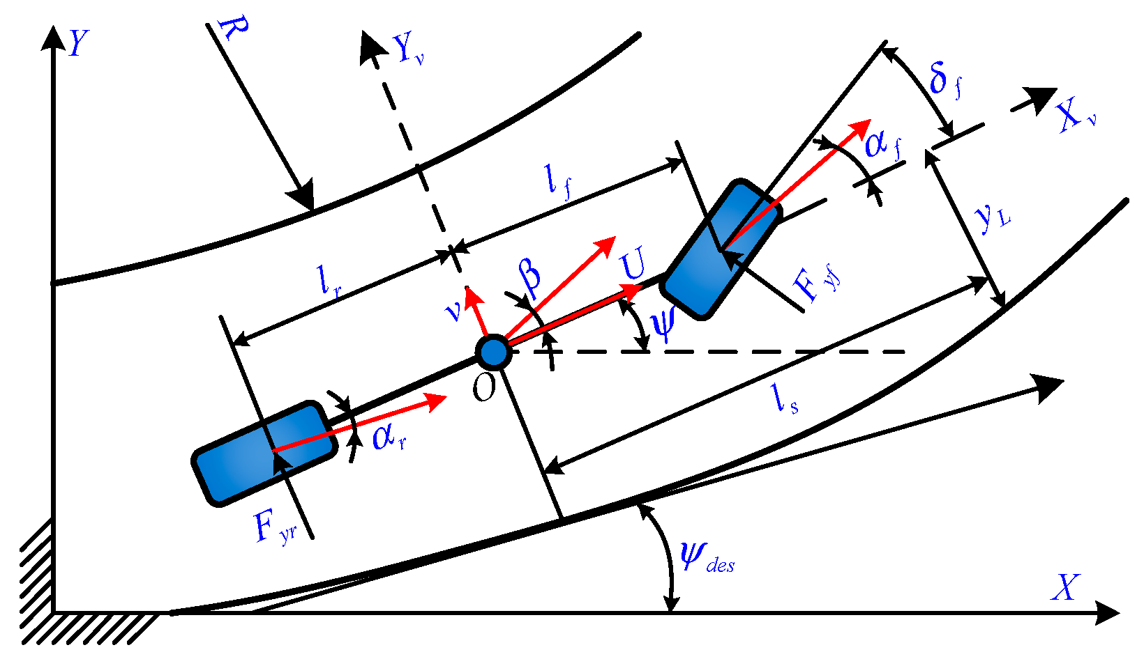
2.1. Vehicle Dynamic Error Tracking Model

It is essential to analyze the trajectory tracking problem to study vehicle lateral dynamics since the vehicle system is an unknown, complicated system with substantial nonlinearity and hysteresis. The vehicle dynamics model is reduced in this work to a two-degree-of-freedom lateral dynamics model for error modeling. Approximations are simplified based on the modeling. The lateral force and the lateral acceleration are roughly proportionate to the tire’s lateral deflection angle and lateral acceleration, respectively.

In Figure 1, $\phi$is the swing angle of the vehicle (rad); $\beta$is the lateral deviation angle of the center of mass of the vehicle (rad). The black arrow $V_x$is the longitudinal speed of the vehicle (m/s); $V_y$is the lateral speed of the vehicle (m/s); X,Y is the natural coordinate system; R is the radius of vehicle trajectory. The red arrow u indicates the velocity of the vehicle’s center of mass; v denotes the transverse velocity of the center of mass of the vehicle.

With the two-degree-of-freedom vehicle model, the following differential equations are obtained assuming a small wheel turning angle and uniform speed:

$$\left(\begin{array}{c}{\dot{V}}_y\\ \ddot{\phi }\end{array}\right)=\left(\begin{array}{cc}\frac{C_{\alpha f}+C_{\alpha r}}{m{V}_x}& \frac{a{C}_{\alpha f}-b{C}_{\alpha r}}{m{V}_x}-V_x\\ \frac{a{C}_{\alpha f}-b{C}_{\alpha r}}{I{V}_x}& \frac{a^2{C}_{\alpha f}+b^2{C}_{\alpha r}}{I{V}_x}\end{array}\right)\left(\begin{array}{c}{V}_y\\ \dot{\phi }\end{array}\right)+\left(\begin{array}{c}-\frac{C_{\alpha f}}{m}\\ -\frac{a{C}_{\alpha f}}{I}\end{array}\right){\delta }_f$$

(1)

where $m$ is the mass of the vehicle (kg); $a,b$is the distance from the center of mass to the front and rear axes (m); $C_{\alpha f }$, $C_{\alpha r}$ is the lateral stiffness of the front and rear wheels (N/rad); and $I$ is the rotational moment of inertia of the center of mass about the Z-axis (kg∙m²).

When the vehicle is under transverse control, the transverse error $e_d$ as well as the cross-swing error $e_{\phi }$ are expected to converge to zero as much as possible to ensure the safety and stability of the tracking control. The lateral and longitudinal decoupling is carried out in the Frenet coordinate system and calculated:

$${\dot{e}}_d=\left|\stackrel{\rightharpoonup }{V}\right|\sin \left(\beta +\phi -{\theta }_r\right)$$

(2)

$${\theta }_r=\theta +{\kappa }_r{e}_s$$

(3)

where $\left|\overline{V}\right|$ is the center-of-mass velocity of the vehicle (m/s); ${\theta }_r$ is the reference heading angle at the current moment (rad); $\theta$is the heading angle of the matching point (rad); $e_s$is the longitudinal error (m); $k_r$is the curvature of the matching point.

The first-order derivative and second-order derivative of the simplified transverse error $e_d$ by the decomposition of coordinate vectors with a small angle assumption are, respectively:

$${\dot{e}}_d=V_y+V_x\left(\phi -{\theta }_r\right)=V_y+V_x{e}_{\phi }$$

(4)

$${\ddot{e}}_d={\dot{V}}_y+V_x{\dot{e}}_{\phi }$$

(5)

The general road curvature change is relatively small, ignoring ${\ddot{\theta }}_{r }$, and the transverse pendulum error and its derivatives are, respectively:

$$e_{\phi }=\phi -{\theta }_r$$

(6)

$${\dot{e}}_{\phi }=\dot{\phi }-{\dot{\theta }}_r$$

(7)

$${\ddot{e}}_{\phi }=\ddot{\phi }$$

(8)

Substituting Equations (4), (5), (7), and (8) into (1) yields a dynamic error tracking model of the vehicle in the natural coordinate system:

$$\left(\begin{array}{c}{\dot{e}}_d\\ {\ddot{e}}_d\\ {\dot{e}}_{\phi }\\ {\ddot{e}}_{\phi }\end{array}\right)=\left(\begin{array}{cccc}0& 1& 0& 0\\ 0& \frac{C_{\alpha f}+C_{\alpha r}}{m{V}_x}& -\frac{C_{\alpha f}+C_{\alpha r}}{m}& \frac{a{C}_{\alpha f}-b{C}_{\alpha r}}{m{V}_x}\\ 0& 0& 0& 1\\ 0& \frac{a{C}_{\alpha f}-b{C}_{\alpha r}}{I{V}_x}& -\frac{a{C}_{\alpha f}-b{C}_{\alpha r}}{I}& \frac{a^2{C}_{\alpha f}+b^2{C}_{\alpha r}}{I{V}_x}\end{array}\right)\left(\begin{array}{c}{e}_d\\ {\dot{e}}_d\\ e_{\phi }\\ {\dot{e}}_{\phi }\end{array}\right)+\left(\begin{array}{c}0\\ -\frac{C_{\alpha f}}{m}\\ 0\\ -\frac{a{C}_{\alpha f}}{I}\end{array}\right){\delta }_f+\left(\begin{array}{c}0\\ \frac{a{C}_{\alpha f}-b{C}_{\alpha r}}{m{V}_x}-V_x\\ 0\\ \frac{a^2{C}_{\alpha f}+b^2{C}_{\alpha r}}{I{V}_x}\end{array}\right){\dot{\theta }}_r$$

Thus, the state space is obtained as

$${\dot{e}}_r=A{e}_r+Bu+C{\dot{\theta }}_r$$

(9)

Among them:

$$A=\left(\begin{array}{cccc}0& 1& 0& 0\\ 0& \frac{C_{\alpha f}+C_{\alpha r}}{m{V}_x}& -\frac{C_{\alpha f}+C_{\alpha r}}{m}& \frac{a{C}_{\alpha f}-b{C}_{\alpha r}}{m{V}_x}\\ 0& 0& 0& 1\\ 0& \frac{a{C}_{\alpha f}-b{C}_{\alpha r}}{I{V}_x}& -\frac{a{C}_{\alpha f}-b{C}_{\alpha r}}{I}& \frac{a^2{C}_{\alpha f}+b^2{C}_{\alpha r}}{I{V}_x}\end{array}\right)$$

$$B=\left(\begin{array}{c}0\\ -\frac{C_{\alpha f}}{m}\\ 0\\ -\frac{a{C}_{\alpha f}}{I}\end{array}\right)C=\left(\begin{array}{c}0\\ \frac{a{C}_{\alpha f}-b{C}_{\alpha r}}{m{V}_x}-V_x\\ 0\\ \frac{a^2{C}_{\alpha f}+b^2{C}_{\alpha r}}{I{V}_x}\end{array}\right)$$

2.2. Continuous Error State Space

Consider that the optimal control problem can be defined abstractly as a function of the objective to minimize the trajectory tracking error, subject to the vehicle dynamic model, control input limitations, and environmental factor constraints, while taking into account the phase constraints to ensure that the implementation of the control strategy does not lead to unstable vehicle behavior.

$$Minimize=J\left(X\left(t\right),U\left(t\right)\right)$$

(10)

Subject to:

$$X_{t+1}=f\left(x_t,u_t\right)$$

(11)

The discretization of Equation (8) starts by neglecting ${\dot{C\theta }}_r$, and integrating both sides of the equation simultaneously:

$${\displaystyle {\int }_t^{t+dt}{\dot{e}}_{r}dt={\displaystyle {\int }_t^{t+dt}\left(A{e}_r+Bu\right)}}dt$$

(12)

Through the integral median theorem as well as Euler’s formula:

$$X(t+dt)={(I-Adt/2)}^{(-1)}(I+Adt/2)X(t)+BdtU(t)$$

(13)

where $I$ is the unit matrix and $dt$ is the sampling time (s).

The state space equation tracking error of the discrete vehicle model can be expressed as

$$X_{k+1}=\overline{A}{X}_k+\overline{B}{u}_k$$

(14)

where

$$\overline{A}={(I-Adt/2)}^{-1}(I+Adt/2)$$

$$\overline{B}=Bdt$$

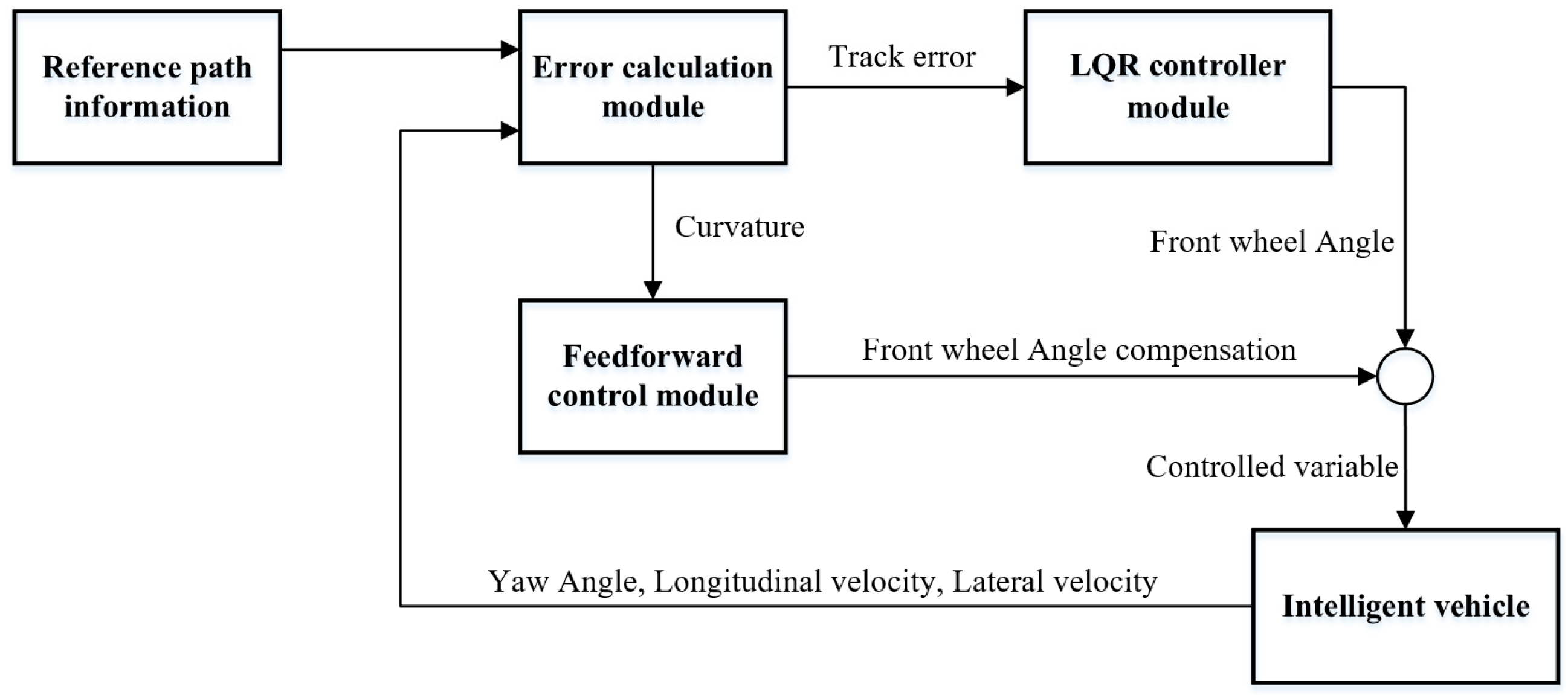
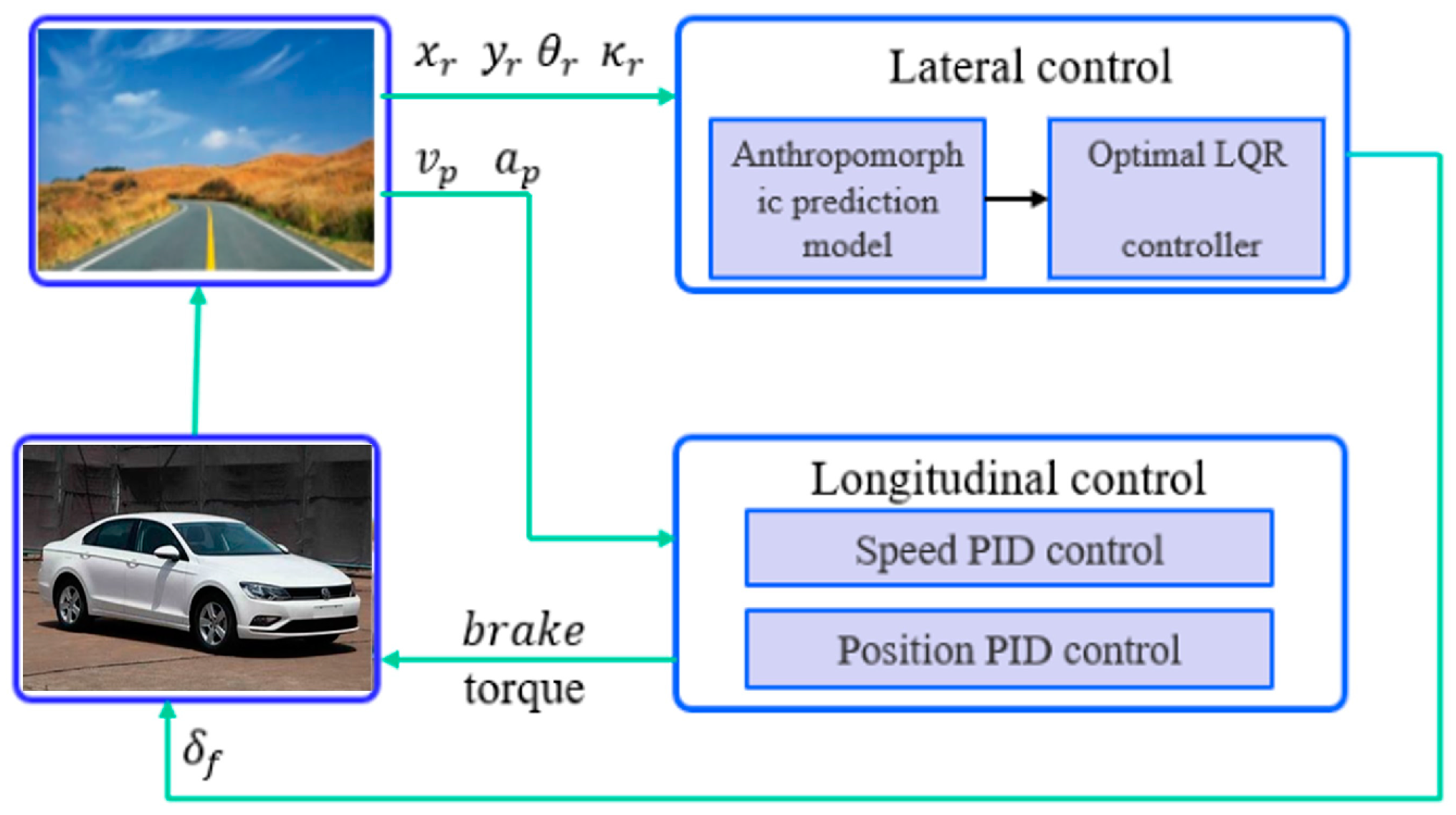
3. Lateral Trajectory Tracking Controller Design

Based on the intelligent vehicle lateral tracking error model, the lateral controller shown in Figure 2 is designed to suppress the distance error and heading error during the tracking process and eliminate the state error between the current position of the intelligent vehicle and the reference position.

3.1. Design of an Optimal Controller

Using LQR in lateral trajectory tracking control can ensure vehicle driving stability when the vehicle deviates from the equilibrium state. Therefore, LOR control in intelligent driving can realize closed-loop optimal control through state feedback. Based on the two-degree-of-freedom differential equations of the vehicle established above, the lateral velocity and the transverse angular velocity are taken as the system’s state variables, and the front wheel angle is taken as the input variable of the system. Based on the discrete vehicle state space equation established by Equation (13) in the previous section, the cost function of the LOR controller is constructed as

$$J={\displaystyle {\sum }_{k=0}^{+\infty }(X_k^{T}Q{X}_k+u_k^{T}R{u}_k)}$$

(15)

where $X_k$ is the state variable of the system, $u_k$ is the control quantity of the system, $Q$is the weighting matrix of the state errors, and $R$ is the weighting matrix of the control inputs.

The Lagrange multiplier method is used to solve Equation (14) for the minima under the constraints of Equation (13):

$$\begin{array}{l}J={\displaystyle {\sum }_{k=0}^{n-1}(X_k^{T}Q{X}_k+u_k^{T}R{u}_k)}+X_n^{T}Q{X}_n\\ +{\displaystyle {\sum }_{k=0}^{n-1}{\lambda }_{k+1}^T}(\overline{A}{X}_k+\overline{B}{u}_k-X_{k+1})\end{array}$$

(16)

The simplification yields:

$$u_k=-{(R+B^T{P}_{k}B)}^{-1}{B}^T{P}_{k+1}A{x}_k$$

(17)

where $P_k=Q+A^T{P}_k{(I+B{R}^{-1}{B}^T{P}_k)}^{-1}A$ is the Riccati equation and $X_K$ represents the error.

The optimal sequence of feedback control is obtained by iterative solving, and the control quantities of the LQR controller for intelligent driving vehicles are obtained as

$$u_k=-k{X}_k$$

(18)

where $k={(R+B^T{P}_{k+1}B)}^{-1}{B}^T{P}_k$ is the feedback gain of the LQR controller.

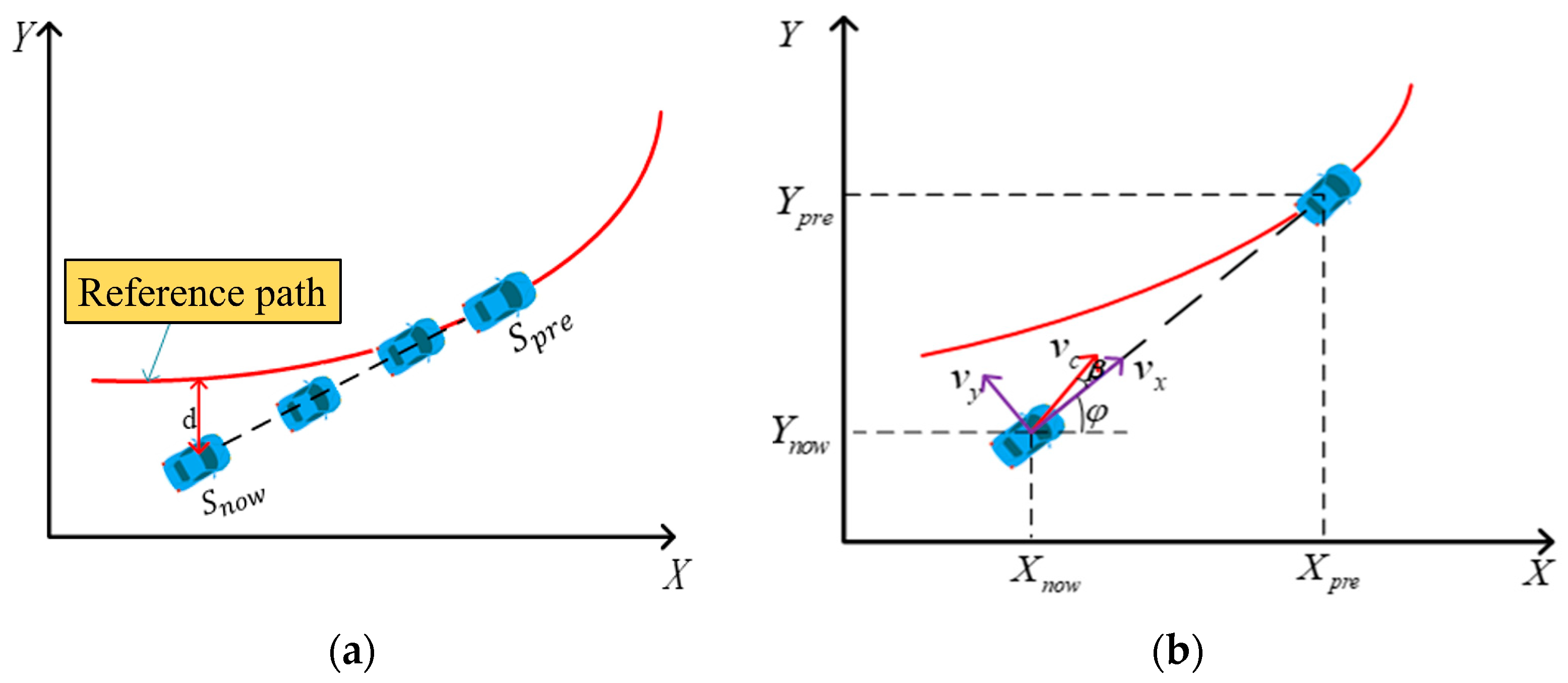
3.2. Anthropomorphic Prediction Module

3.2.1. Feedforward Control Design

At this point, the controller will have some steady state error, which requires the use of the previously ignored $\dot{C{\theta }_r}$ to calculate the amount of feedforward control.

$${\dot{e}}_{rr}=\left(A-BK\right)e_{rr}\cdot C{\dot{\theta }}_r$$

(19)

Introduce feedforward control and wait for the system to stabilize:

$$e_{rr}=-{(A-BK)}^{-1}(B{\delta }_a+C{\dot{\theta }}_r)=0$$

(20)

where ${\delta }_a$is the amount of feedforward control.

$$e_{rr}=\left(\begin{array}{c}\frac{1}{k_1}({\delta }_a-\frac{{\dot{\theta }}_r}{V_x}(a+b-b{k}_3-\frac{m{V_x}^2}{a+b}(\frac{b}{C_{\alpha f}}+\frac{a}{C_{\alpha r}}{k}_3-\frac{a}{C_{\alpha r}})))\\ 0\\ -\frac{{\dot{\theta }}_r}{V_x}(b+\frac{a}{a+b}\frac{m{V_x}^2}{C_{\alpha r}})\\ 0\end{array}\right)$$

When ${\delta }_a=\frac{{\dot{\theta }}_r}{V_x}(a+b-b{k}_3-\frac{m{V_x}^2}{a+b}(\frac{b}{C_{\alpha f}}+\frac{a}{C_{\alpha r}}{k}_3-\frac{a}{C_{\alpha r}})$, lateral displacement error is equal to zero, where $k=\left[\begin{array}{cccc}{k}_1& k_2& k_3& k_4\end{array}\right]$ is the feedback matrix.

As

$${\dot{\theta }}_r=k_r\cdot v_x$$

(21)

Equation (20) is brought into the feedforward control to obtain

$${\delta }_a=k_r(a+b-b{k}_3-\frac{m{V_x}^2}{a+b}(\frac{b}{C_{\alpha f}}+\frac{a}{C_{\alpha f}}{k}_3-\frac{a}{C_{\alpha r}}))$$

(22)

$$k_r(t)=\frac{y^{″}\cdot x\left(t\right)}{{\left(1+y^{\prime }\cdot x{\left(t\right)}^2\right)}^{\frac{3}{2}}}$$

(23)

where $k_r$ is the curvature of the projection point.

In summary, the control volume of the whole system can be obtained as

$$U=-k{e}_{rr}+{\delta }_a$$

(24)

3.2.2. Anthropomorphic Prediction Module

As shown in Figure 3a,b, $S_{now }$is the current location of the driverless car, $S_{pre }$ is the prediction point, and $d$ is the lateral error between the current moment and the reference trajectory. In the case of someone’s cab, the driver will predict the future path for efficient and accurate trajectory tracking in time, the current moment, and the reference path error; the driver will not turn the steering wheel, the future moments will be able to drive into the reference trajectory, and the algorithm can only mechanically calculate the current moment of the position and the matching point of the existence of the error, for the front wheels of the corner control, but not predict the future reference path. Therefore, adding the prediction module can solve the lag of the controller, offset the delay, and improve the driving efficiency.

The prediction time is set to $t_s$, replacing the information of the current point with the information of the predicted point, as can be seen in Figure 3b:

$$x_{pre}=x+(V_x{t}_s+\frac{1}{2}{a}_x{t}_s^2)\cos \phi -(V_y{t}_s+\frac{1}{2}{a}_y{t}_s^2)\sin \phi$$

(25)

$$y_{pre}=y+(V_y{t}_s+\frac{1}{2}{a}_y{t_s}^2)\cos \phi -(V_x{t}_s+\frac{1}{2}{a}_x{t}_s^2)\sin \phi$$

(26)

$${\phi }_{pre}=\phi +\dot{\phi }{t}_s$$

(27)

$$v_{x_{pre}}=v_x v_{y_{pre}}=v_y$$

(28)

where $a_x$ is the longitudinal acceleration and $a_y$ is the lateral acceleration.

The main parameter values of the lateral controller are shown in

Table 1. Main parameter values of the lateral controller.

Symbol	Value	Unite
a	1015	mm
b	1895	mm
m	1270	$\mathrm{kg}$
I	1536.71	$\mathrm{kg}·{\mathrm{m}}^2$
$C_{\partial f}$	124,760	N/rad
$C_{\partial r}$	85,200	N/rad

:

3.3. Lateral Velocity Viewer Design

In trajectory tracking control research, it is impossible to observe the lateral velocity of intelligent vehicles due to the lack of lateral velocity sensors. Thus, numerous lateral speed observation algorithms are derived, and different algorithms have different advantages. The Luenberger observer utilizes the pole configuration method to freely set the bandwidth of the observer, which is widely used in engineering technology [36]. Firstly, the observation error equation is established according to the vehicle two-degree-of-freedom model and the Luenberger observer to analyze the source of uncertainty of the observation error; secondly, by setting up the observation feedback gain L-matrix, to achieve error compensation and optimize the observer bandwidth. The Luenberger observer with gain matrix L mainly consists of the gain matrix L and the observer state-space equation is based on the vehicle’s two degrees of freedom, as shown in Figure 4.

Luenberger Observer with Gain Matrix L

In this section, a closed-loop Luenberger observer is chosen for lateral velocity observations to improve the accuracy of the estimation of the parameters. A CarSim real-time vehicle model is used instead of an actual vehicle, and to analyze the characteristics of the observer, a two-degree-of-freedom vehicle model will be used:

$$\left\{\begin{array}{l}\dot{x}=Ax+Bu\hfill \\ y=Cx+Du\hfill \end{array}\right.$$

(29)

where x is the state quantity of the CarSim vehicle model containing the transverse angular velocity and lateral velocity of the sensor outputs, A, B, C, and D are the matrices of state-space equation coefficients of the approximate two-degree-of-freedom model, and the inputs are$\delta$.

Similarly, the state space equations of the observer are simplified to the same form as for the two-degree-of-freedom model of the vehicle:

$$\left\{\begin{array}{l}\dot{\tilde{x}}=\tilde{A}x+\tilde{B}u+L(y-\tilde{y})\hfill \\ \tilde{y}=\tilde{C}x+\tilde{D}u\hfill \end{array}\right.$$

(30)

The observer error equation is established based on the state space equation of the Lomborg observer with CarSim:

$$\left(\dot{\tilde{x}}-\dot{x}\right)=\left(\tilde{A}-L\tilde{C}\right)\left(\tilde{x}-x\right)+\mathsf{\Delta }Ax+\mathsf{\Delta }Bu+L\mathsf{\Delta }Cx+L\mathsf{\Delta }Du$$

(31)

where $\mathsf{\Delta }Ax+\mathsf{\Delta }Bu+L\mathsf{\Delta }Cx+L\mathsf{\Delta }Du$ is generated by parameter uncertainty. In order to reduce the effect of parameter uncertainty and the amplification of the error by the observer, the amount of error in each error matrix will be specifically analyzed in the following equation:

$$\begin{array}{l}\mathsf{\Delta }A=\left[\begin{array}{cc}\mathsf{\Delta }\left(\frac{C_{\alpha f}+C_{\alpha r}}{m{v}_x}\right)& \mathsf{\Delta }\left(\frac{a{C}_{\alpha f}-b{C}_{\alpha r}}{m{v}_x}\right)\\ \mathsf{\Delta }\left(\frac{a{C}_{\alpha f}-b{C}_{\alpha r}}{I{v}_x}\right)& \mathsf{\Delta }\left(\frac{a^2{C}_{\alpha f}+b^2{C}_{\alpha r}}{I{v}_x}\right)\end{array}\right]\mathsf{\Delta }B=\left[\begin{array}{c}-\frac{\mathsf{\Delta }{C}_{\alpha f}}{m}\\ -\frac{a\mathsf{\Delta }{C}_{\alpha f}}{I}\end{array}\right] \\ \mathsf{\Delta }C=\left[\begin{array}{cc}0& 0\\ \mathsf{\Delta }\left(\frac{C_{\alpha f}+C_{\alpha r}}{m{v}_x}\right)& \mathsf{\Delta }\left(\frac{a{C}_{\alpha f}-b{C}_{\alpha r}}{m{v}_x}\right)\end{array}\right] \mathsf{\Delta }D=\left[\begin{array}{c}0\\ -\frac{\mathsf{\Delta }{C}_{\alpha f}}{m}\end{array}\right]\end{array}$$

(32)

Parameter uncertainty analysis does not analyze every parameter, but analyzes the elements in the parameter error matrix and turns them into the comprehensive error of many elements, which is convenient ffor the subsequent calculation and design. Split the state space equation into lateral velocity and transverse pendulum angular velocity, and specifically analyze the role of different elements of the feedback matrix L in the two states. According to the analysis, the following can be obtained.

Conclusion 1: When $L_{12}=0.5\sim 1.0$, where $L_{12}$ is the first row and second column elements of the L matrix, which can minimize the error caused by the uncertainty of the parameters, the specific analysis process is as follows:

$$\begin{array}{ll}{\dot{\tilde{v}}}_y-{\dot{v}}_y& =(1-l_{12})\frac{C_{\alpha f}+C_{\alpha r}}{m{v}_x}({\tilde{v}}_y-v_y)\\ & +\left(\frac{a{C}_{\alpha f}-b{C}_{\alpha r}}{m{v}_x}(1-l_{12})-v_x-l_{11}\right)(\tilde{\phi }-\phi )\\ & +\mathsf{\Delta }\left(\frac{C_{\alpha f}+C_{\alpha r}}{m{v}_x}\right)v_y+\mathsf{\Delta }\left(\frac{a{C}_{\alpha f}-b{C}_{\alpha r}}{m{v}_x}\right)\phi +\left(-\frac{\mathsf{\Delta }{C}_{\alpha f}}{m}\right)u\\ & -l_{12}\mathsf{\Delta }\left(\frac{C_{\alpha f}+C_{\alpha r}}{m{v}_x}\right)v_y-l_{12}\mathsf{\Delta }\left(\frac{a{C}_{\alpha f}-b{C}_{\alpha r}}{m{v}_x}\right)r-l_{12}\left(-\frac{\mathsf{\Delta }{C}_{\alpha f}}{m}\right)u\end{array}$$

(33)

By analyzing the error equation for lateral velocity separately, the above setting of the magnitude of $L_{12}$ affects the magnitude of the lateral velocity error, which can play the role of feedforward compensation and also reduces the effect of parameter uncertainty in the lateral velocity error equation.

Conclusion 2: When $L_{22}=0$, where $L_{22}$ is the second row and second column element of the L matrix, which can reduce the error caused by parameter uncertainty, the specific analysis process is as follows:

$$\begin{array}{ll}\dot{\tilde{\phi }}-\dot{\phi }& =\left(\frac{a{C}_{\alpha f}-b{C}_{\alpha r}}{I{v}_x}-l_{22}\frac{C_{\alpha f}+C_{\alpha r}}{m{v}_x}\right)({\tilde{v}}_y-v_y)\\ & +\left(\frac{a^2{C}_{\alpha f}+b^2{C}_{\alpha r}}{I{v}_x}-l_{22}\frac{a{C}_{\alpha f}-b{C}_{\alpha r}}{m{v}_x}-l_{21}\right)(\tilde{r}-r)\\ & +\mathsf{\Delta }\left(\frac{a{C}_{\alpha f}-b{C}_{\alpha r}}{I{v}_x}\right)v_y+\mathsf{\Delta }\left(\frac{a^2{C}_{\alpha f}+b^2{C}_{\alpha r}}{I{v}_x}\right)r+\mathsf{\Delta }\left(-\frac{a\mathsf{\Delta }{C}_{\alpha f}}{I}\right)u\\ & -l_{22}\mathsf{\Delta }\left(\frac{C_{\alpha f}+C_{\alpha r}}{m{v}_x}\right)Vy-l_{22}\mathsf{\Delta }\left(\frac{a{C}_{\alpha f}-b{C}_{\alpha r}}{m{v}_x}\right)r-l_{22}\left(-\frac{\mathsf{\Delta }{C}_{\alpha f}}{m}\right)u\end{array}$$

(34)

By analyzing the error equation for the transverse pendulum angular velocity separately, the size of $L_{22}$ mentioned above ensures the convergence speed of the transverse pendulum angular velocity. It achieves a rapid reduction in error.

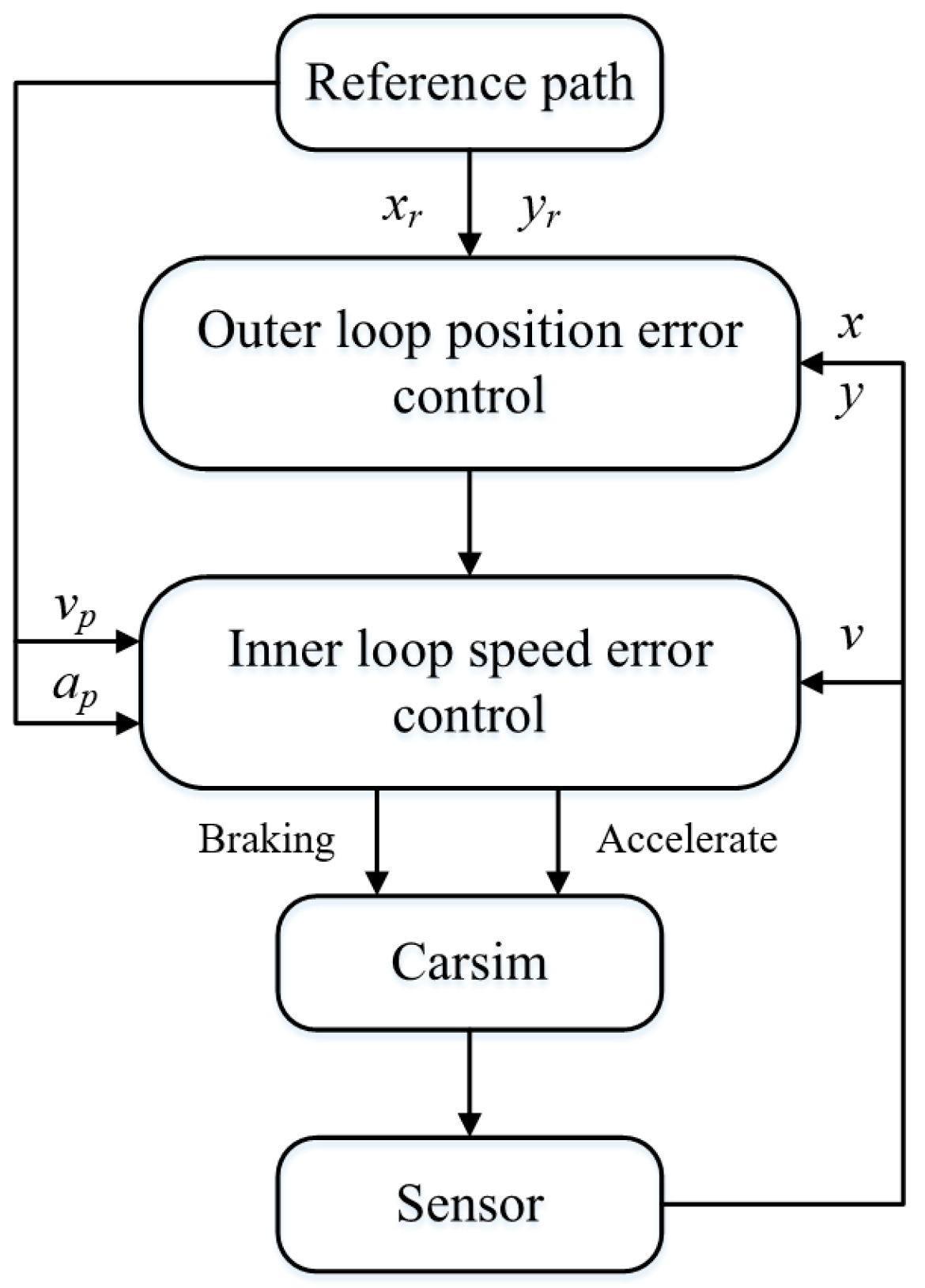
4. Longitudinal Controller Design

To ensure that the vehicle can travel along the target path, longitudinal tracking control and lateral control are required. In the longitudinal tracking control, to meet the speed tracking conditions, this paper will add longitudinal position error for PID control to the speed PID control so that the position and longitudinal speed are in the ideal range.

$$e_v=v_p-\dot{s}$$

(35)

$$V_p=\sqrt{{\dot{x}}_r+{\dot{y}}_r}$$

(36)

$$a_p=\sqrt{{\ddot{x}}_r+{\ddot{y}}_r}$$

(37)

$$\dot{s}=\frac{V_x\cos \left(\phi -{\theta }_r\right)-V_y\sin \left(\phi -{\theta }_r\right)}{1-{\kappa }_r{e}_d}$$

(38)

where $e_v$ is the longitudinal error (m); $\dot{s }$ is the longitudinal velocity (m/s); $a_p$ is the desired acceleration (m/s²).; and $x_r,y_{r }$is the planning point.

The longitudinal tracking control framework diagram is shown in Figure 5:

For the setting of the above two controller parameters, the position of the outer loop controller plays a role in compensating for the speed controller, so the coefficient should not be too large; among the speed controllers, the speed change should be kept continuous, and the change is not easy to be too large, so the coefficient size of the speed controller can be set moderately. The optimal controller parameters can be obtained through repeated parameter adjustments.

Combining the above transverse and longitudinal controls, the trajectory tracking controller is designed as shown in Figure 6.

5. Simulation Verification

5.1. Software Simulation Verification and Analysis

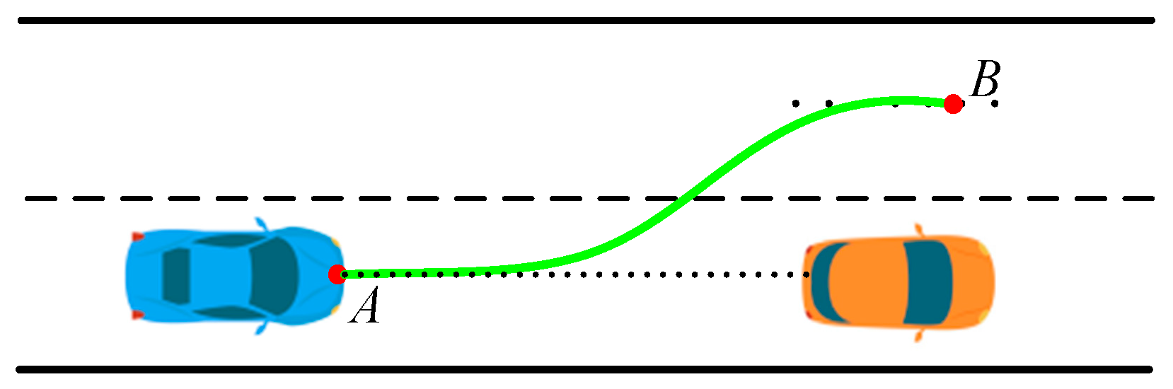
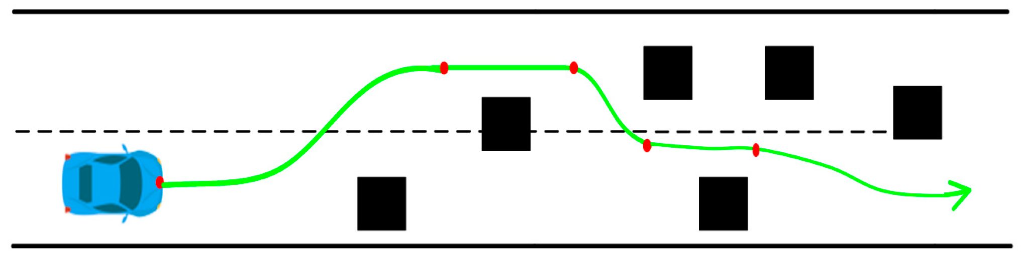
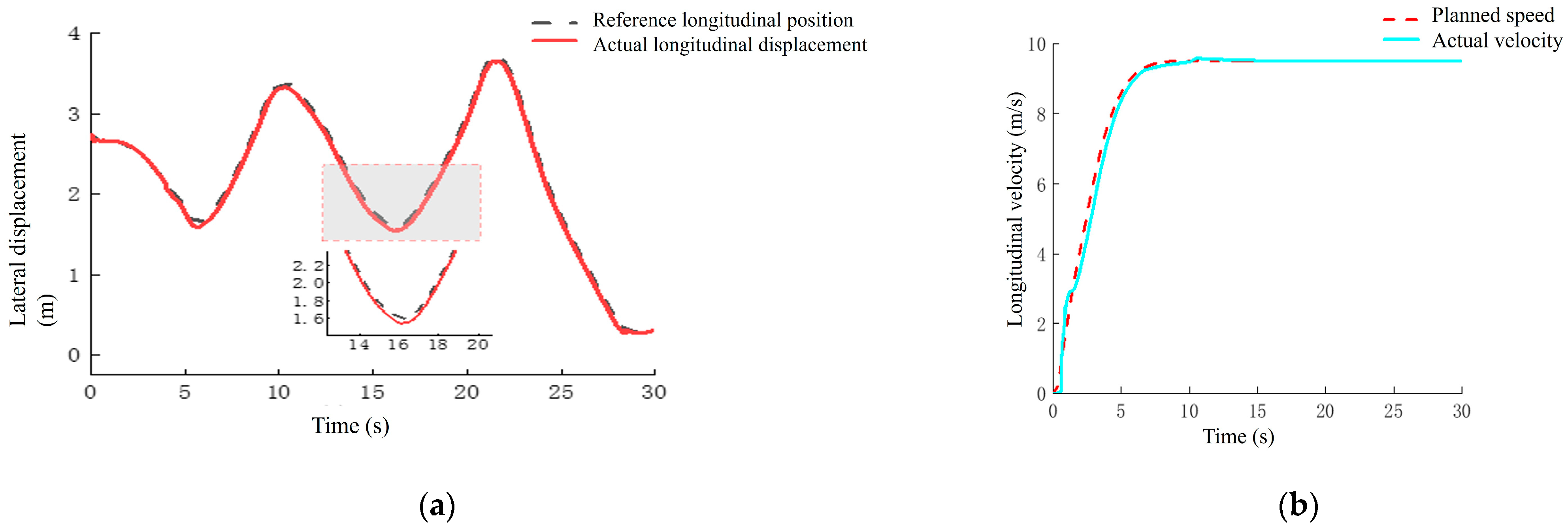
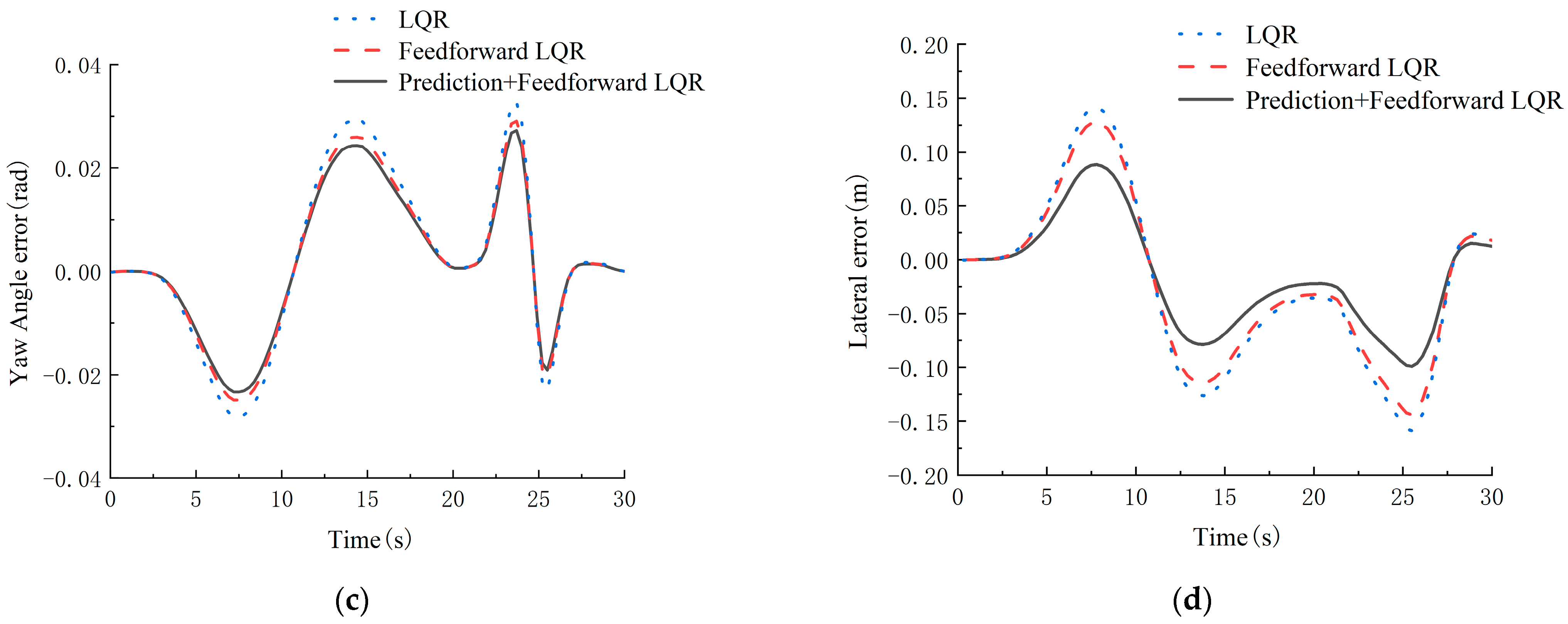
5.1.1. Experimental Verification of Trajectory Tracking Simulation

To verify the performance of the designed tracking algorithm, the dynamics model of the vehicle is modeled using Carsim2019.0 software, and the control system is simulated using Matlab/Simulink2021b software for joint simulation of the control system integration and vehicle dynamics model. Three horizontal control strategies using traditional linear quadratic regulator (LQR), feedforward LQR, and prediction+feedforward LQR as comparisons, and two vertical control strategies using traditional PID and double PID as comparisons are selected, aiming to demonstrate the effectiveness of the proposed anthropomorphic look-ahead reference path and longitudinal speed closed-loop control strategies in the enhancement of the trajectory tracking accuracy and stability of the intelligent vehicles through the comparisons of different methods.

The path in Figure 7, Case 1, is used as the reference path for simulation experiments to verify.

In Figure 7, the dashed line indicates the distance between the vehicle and the vehicle in front of it. The green line indicates the reference path of the vehicle. A is the starting point of the vehicle and B is the target point.

Figure 8 shows the trajectory tracking simulation results for Case 1. Figure 8a shows the longitudinal displacement curve. As shown in the figure, both the PID controller and double-PID controller can track the longitudinal displacement well, but it can be seen that the longitudinal tracking error of the vehicle with double-PID control is smaller and more accurate. Figure 8b shows the transverse displacement curve. As shown in the figure, the LQR controller, feedforward LQR controller, and prediction + feedforward LQR controller can track the transverse displacement very well, but it can be seen that the vehicle transverse trajectory tracking error of the prediction + feedforward LQR control is smaller compared to the other two control methods, and the accuracy is more accurate and more satisfied with the expected value. Figure 8c shows the traverse angle error curve. The traverse angle error at the peak of the LQR controller is 0.030 rad/s, the traverse angle error at the peak of the feedforward LQR controller is 0.029 rad/s, and the traverse angle error at the peak of the predictive+feedforward LQR controller is 0.025 rad/s. Through comparative analysis, the predictive+feedforward controller has a 16.7% reduction in error compared with that of the LQR controller, and the predictive+feedforward controller has a 16.7% reduction in error compared with that of the LQR controller. By comparison, the error of the prediction+feedforward controller is reduced by 16.7% and the error of the prediction+feedforward controller is reduced by 13.8% compared with the feedforward LQR controller, and the error in the whole tracking process is less than 0.03 rad/s. The error meets the theoretical requirement and satisfies the stability of the vehicle. Figure 8d shows the lateral error curve: the lateral displacement error at the peak of the LQR controller is 0.135 m, the maximum lateral displacement error at the peak of the feedforward LQR controller is 0.124, and the maximum lateral displacement error at the peak of the prediction+feedforward LQR controller is 0.078 m. The prediction+feedforward LQR controller decreases the error by 42.2% compared to the LQR controller, and the prediction+feedforward LQR controller decreases the error by 13.8% compared to the LQR controller, and the prediction+feedforward LQR controller decreases the error by 13.8% compared to the LQR controller. Prediction+feedforward LQR controller reduces the error by 37.1% compared to the feedforward LQR controller, and the error is less than 0.1 m during the whole tracking process, which not only ensures the smoothness of the vehicle traveling but also ensures sufficient tracking accuracy.

The path in Figure 9, Case 2, is taken as the reference path for simulation experiments to verify.

In Figure 9, the black square indicates the obstacles on the path. The green line indicates the reference path of the vehicle.

Figure 9 shows the trajectory tracking simulation results for Case 2. In Figure 10a, the red solid line is the actual lateral position, and the dashed line indicates the desired lateral position, from which it can be seen that the lateral position error is within a reasonable range, and continuous obstacle avoidance can be performed. In Figure 10b, the solid line is the actual longitudinal speed of the vehicle, and the dashed line is the desired longitudinal speed, from which it can be seen that its longitudinal speed can also track up the desired speed better. Figure 10c shows the traverse angle error curve. The traverse angle error at the peak of the LQR controller is 0.033 rad/s, the traverse angle error at the peak of the feedforward LQR controller is 0.029 rad/s, and the traverse angle error at the peak of the prediction+feedforward LQR controller is 0.028 rad/s. Through the comparative analysis, the prediction+feedforward controller reduces 15.2% of the traverse angle error compared with that of the LQR controller, and the prediction+feedforward controller reduces 15.2% of the error compared with that of the LQR controller. reduced by 15.2%, and the error of the prediction+feedforward controller is reduced by 3.5% compared to that of the feedforward LQR controller, and the error in the whole tracking process is less than 0.04 rad/s. It meets the theoretical requirement error and satisfies the stability of the vehicle. Figure 10d shows the lateral error curve: the lateral displacement error at the peak of the LQR controller is 0.148 m, the maximum lateral displacement error at the peak of the feedforward LQR controller is 0.147, the maximum lateral displacement error at the peak of the prediction+feedforward LQR controller is 0.098 m, and the prediction+feedforward LQR controller reduces the error by 38.0% compared to the LQR controller, the prediction+feedforward LQR controller reduces the error by 3.5% compared to the LQR controller, and the prediction+feedforward LQR controller reduces the error by 3.5% compared to the LQR controller. feedforward LQR controller reduces the error by 33.3% compared to the feedforward LQR controller, and the error is less than 0.01 m throughout the tracking process, which not only ensures the smoothness of the vehicle traveling but also ensures sufficient tracking accuracy.

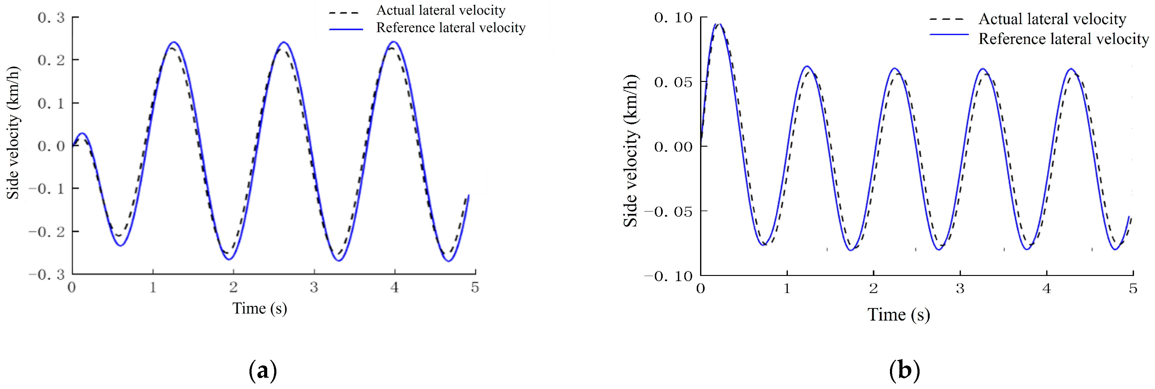
5.1.2. Experimental Validation of Lateral Observer Simulation

To verify the effectiveness of the observer, CarSim and MATLAB/Simulink are utilized for joint simulation to set different steering frequencies, and the estimation algorithm of lateral velocity has a strong tracking performance. The simulation results are plotted in Figure 11.

As shown in Figure 10a,b, the accuracy of the lateral velocity observation algorithm is verified under different steering frequencies. It can be seen from the simulation graphs that when the steering wheel is rotated faster, the lateral velocity performance decreases slightly. However, it is also within a reasonable range. From the above simulation results, it can be seen that the Lomburg observer with gain matrix L can observe the lateral velocity more accurately.

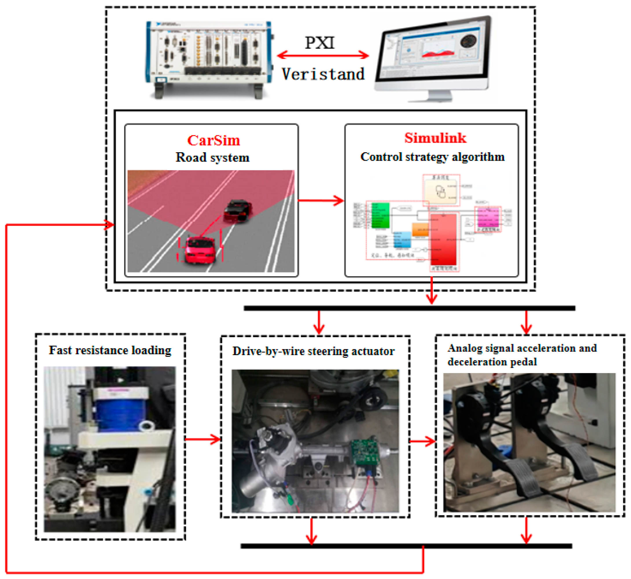
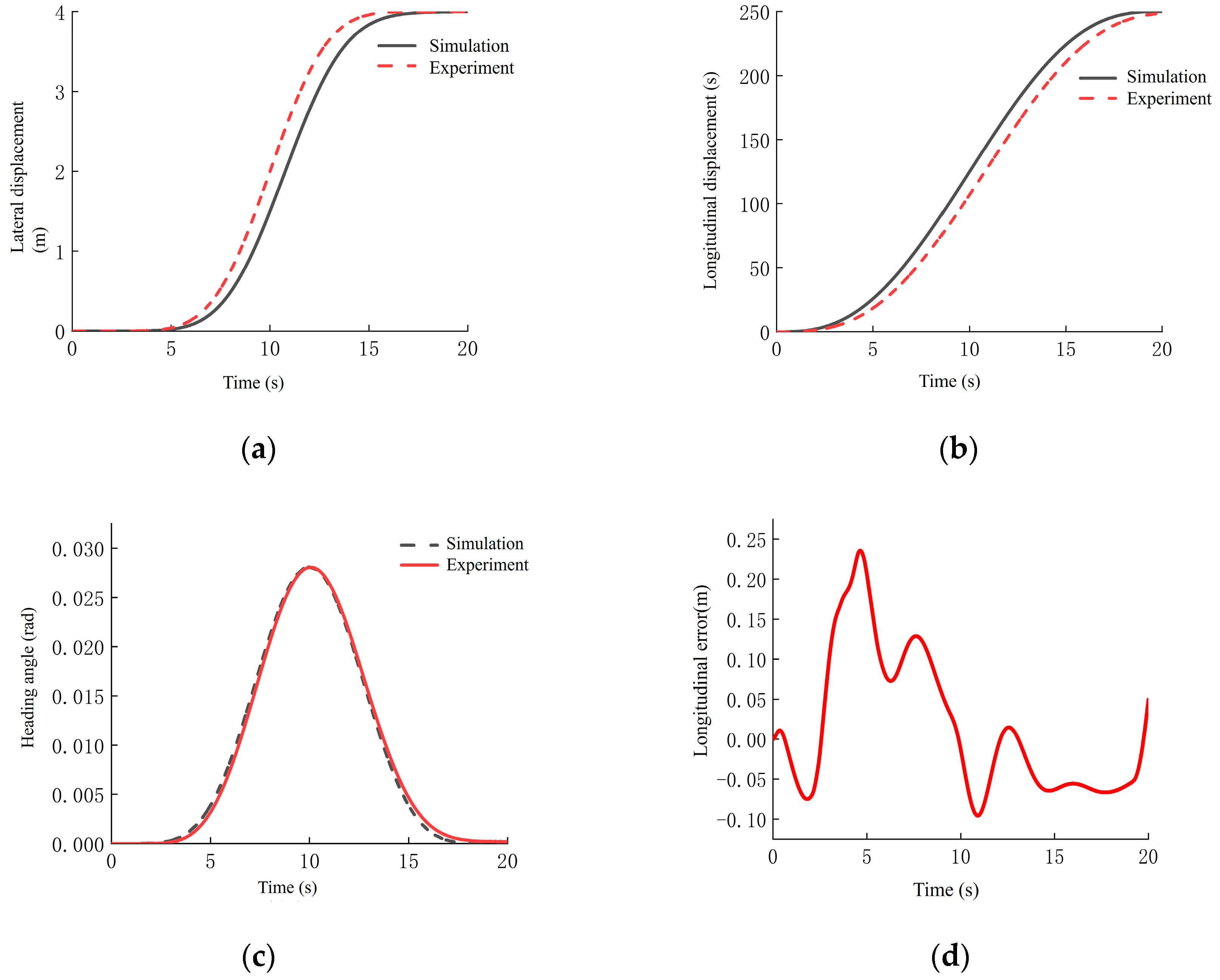
5.2. Hardware-in-the-Loop Simulation Verification and Analysis

Figure 12 shows the schematic diagram of the HIL test in this section. In this HIL system, the vehicle-road system model of CarSim2019.0 and the obstacle avoidance lane change trajectory tracking algorithm are embedded into the PXI real-time system through the upper computer software Veristad2011, which calculates the target steering angle and target acceleration/deceleration signals and sends the control commands to the actuator controller through the CAN bus. Then, the column angle and rotational speed data of the steering system and the pressure data of the brake wheel cylinder are collected by the angle sensor and pressure sensor and sent to the PXI real-time system to realize the closed loop.

The trajectory tracking algorithm was verified and analyzed using a steer-by-wire testbed, as shown in Figure 13.

From the HIL bench test, it can be seen that Figure 13 transverse displacement compared to the software simulation error will become more extensive but also within a reasonable range; the reason for the more significant error may include the controller and the communication of the real-time poor and other situations. The longitudinal and lateral displacements are more similar, but the error is also to meet its requirements. (c) The pendulum angle data collected through the test is closer to the pendulum angle obtained from the simulation, and the maximum error is within 0.002 rad. (d) As shown in (d), the maximum longitudinal position error is about 0.24 m, which also meets the tracking requirements in the longitudinal control.

6. Conclusions

In this paper, a trajectory tracking control method with anthropomorphic horizontal and vertical joint control is studied for intelligent vehicles. To address the problem that most of the current algorithms in the trajectory tracking process require too much computational power from the controller, which makes it difficult to ensure the real-time sensitivity and stability of the control and thus affects the accuracy and stability of the trajectory tracking. Firstly, based on the dynamic tracking error model of the vehicle, an anthropomorphic prediction model of the intelligent vehicle is designed to be combined with the optimal controller for the transverse tracking control algorithm. Secondly, to improve the accuracy of vehicle longitudinal speed tracking, a vehicle speed tracking controller is designed to incorporate longitudinal position error control into speed control. Aiming at the problem that it is difficult to observe the vehicle lateral speed, the vehicle lateral speed observation algorithm is designed according to the vehicle two-degree-of-freedom model and the Luenberger observer to observe the vehicle lateral speed. Finally, two typical working conditions are selected for joint simulation on CarSim2019.0 and MatLab/Simulink2021b software, as well as hardware-in-the-loop testing on a semi-physical experimental platform. The simulation and test results show that the lateral tracking control algorithm designed in this paper can effectively compensate for the system delay and improve the accuracy of the track lateral trail tracking. The speed tracking controller designed in this paper can realize a more accurate and stable speed tracking effect, improve the driving safety and stability of intelligent vehicles in complex road environments, and also provide a new way of thinking for the design of the control system of intelligent vehicles in the future.

This study also has some limitations. The proposed algorithm in the current study has only been verified by software simulation and hardware in-loop testing. The actual effectiveness of the algorithm has not been verified on real vehicles. Therefore, the effectiveness of the algorithm can be further verified for application on real vehicles in future work.

References

1. Akopov, A.S.; Beklaryan, L.A.; Beklaryan, A.L. Simulation-Based Optimisation for Autonomous Transportation Systems Using a Parallel Real-Coded Genetic Algorithm with Scalable Nonuniform Mutation. Cybern. Inf. Technol. 2021, 21, 127–144. [Google Scholar] [CrossRef]
2. Chen, H.; Chen, S.; Gong, J. Research review on lateral control methods for intelligent vehicles. J. Mil. Eng. 2017, 38, 1203–1214. [Google Scholar] [CrossRef]
3. Ji, J.; Khajepour, A.; Melek, W.W.; Huang, Y. Path Planning and Tracking for Vehicle Collision Avoidance Based on Model Predictive Control With Multiconstraints. IEEE Trans. Veh. Technol. 2017, 66, 952–964. [Google Scholar] [CrossRef]
4. Zhang, S.; Zhao, X.; Zhu, G.; Shi, P.; Hao, Y. Adaptive trajectory tracking control strategy of intelligent vehicle. Int. J. Distrib. Sens. Netw. 2020, 16, 5. [Google Scholar] [CrossRef]
5. Li, R.; Yang, Z.; Yan, G.; Jian, L.; Li, G.; Li, Z. Robust Approximate Optimal Trajectory Tracking Control for Quadrotors. Aerospace 2024, 11, 149. [Google Scholar] [CrossRef]
6. Deng, C.; Qian, Y.; Dong, H.; Xu, J.; Wang, W. Lane Change Trajectory Planning Based on Quadratic Programming in Rainy Weather. World Electr. Veh. J. 2023, 14, 252. [Google Scholar] [CrossRef]
7. Wang, W.; Li, G.; Liu, S. Research on Trajectory Tracking Control of a Semi-Trailer Train Based on Differential Braking. World Electr. Veh. J. 2024, 15, 30. [Google Scholar] [CrossRef]
8. Fu, W.; Liu, Y.; Zhang, X. Research on Accurate Motion Trajectory Control Method of Four-Wheel Steering AGV Based on Stanley-PID Control. Sensors 2023, 23, 7219. [Google Scholar] [CrossRef]
9. Li, P.; Zhong, R.; Lu, S. Optimal control scheme of space tethered system for space debris deorbit. ACTA Astrona 2019, 165, 355–364. [Google Scholar] [CrossRef]
10. Hui, S.; Li, Y.; Li, F.; Niu, X. Distributed LQR Optimal Protocol for Leader-Following Consensus. IEEE Trans. Cybern. 2019, 49, 3532–3546. [Google Scholar] [CrossRef]
11. Carlos, O.; Ramon, L.; Abdelali, E.; Isabelle, Q. Robust LQR Control for PWM Converters: An LMI Approach. IEEE Trans. Ind. Electron. 2009, 56, 2548–2558. [Google Scholar] [CrossRef]
12. Sharp, R.S.; Peng, H. Vehicle dynamics applications of optimal control theory: Vehicle System Dynamics. Veh. Syst. Dyn. 2011, 49, 1073–1111. [Google Scholar] [CrossRef]
13. Snider, J.M. Automatic steering methods for autonomous automobile path tracking. In Robotics Institute. CMURITR-09-08; Carnegie Mellon University: Pittsburgh, PA, USA, 2009. [Google Scholar]
14. Xu, S.; Peng, H.; Tang, Y. Preview Path Tracking Control With Delay Compensation for Autonomous Vehicles. IEEE Trans. Intell. Transp. Syst. 2021, 22, 2979–2989. [Google Scholar] [CrossRef]
15. Zhang, Y.; Niu, R.; Wang, J.; Liang, H.; Chen, Z.; Huang, Z. Path Tracking Control Algorithm Considering Delay Compensation. In Proceedings of the 2022 7th Asia-Pacific Conference on Intelligent Robot Systems (ACIRS), Tianjin, China, 1–3 July 2022; pp. 64–69. [Google Scholar]
16. Saif, A.-W.A.; El-Ferik, S.; Elkhider, S.M. Robust Stabilization of Linear Time-Delay Systems under Denial-of-Service Attacks. Sensors 2023, 23, 5773. [Google Scholar] [CrossRef]
17. Okasha, M.; Kralev, J.; Islam, M. Design and Experimental Comparison of PID, LQR and MPC Stabilizing Controllers for ParrotMambo Mini-Drone. Aerospace 2022, 9, 298. [Google Scholar] [CrossRef]
18. Wang, L.; Zhai, Z.; Zhu, Z.; Mao, E. Path Tracking Control of an Autonomous Tractor Using Improved Stanley Controller Optimized with Multiple-Population Genetic Algorithm. Actuators 2022, 11, 22. [Google Scholar] [CrossRef]
19. AbdElmoniem, A.; Osama, A.; Abdelaziz, M.; Maged, S.A. A path-tracking algorithm using predictive Stanley lateral controller. Int. J. Adv. Robot. Syst. 2020, 17, 1729881420974852. [Google Scholar] [CrossRef]
20. Luan, Z.; Zhang, J.; Zhao, W.; Wang, C. Trajectory Tracking Control of Autonomous Vehicle With Random Network Delay. IEEE Trans. Veh. Technol. 2020, 69, 8140–8150. [Google Scholar] [CrossRef]
21. Yu, J.; Guo, X.; Pei, X.; Chen, Z.; Zhou, W.; Zhu, M.; Wu, C. Path tracking control based on tube MPC and time delay motionprediction. IET Intell. Transp. Syst. 2019, 14, 1–12. [Google Scholar] [CrossRef]
22. Xu, S.; Peng, H.; Song, Z.; Chen, K.; Tang, S. Design and test of speed tracking control for the self-driving Lincoln MKZ platform. IEEE Trans. Intell. Veh. 2019, 5, 324–334. [Google Scholar] [CrossRef]
23. Yu, S.; Li, X.; Chen, H.; Allgöwer, F. Nonlinear model predictive control for path following problems. Int. J. Robust Nonlinear Control 2015, 25, 1168–1182. [Google Scholar] [CrossRef]
24. Mayne, D.Q. Model predictive control: Recent developments and future promise. Automatica 2014, 50, 2967–2986. [Google Scholar] [CrossRef]
25. Pang, H.; Liu, N.; Hu, C.; Xu, Z. A practical trajectory tracking control of autonomous vehicles using linear time-varying MPC method. Proc. Inst. Mech. Eng. 2021, 236, 709–723. [Google Scholar] [CrossRef]
26. Xu, S.; Peng, H. Design, Analysis, and Experiments of Preview Path Tracking Control for Autonomous Vehicles. IEEE Trans. Intell. Transp. Syst. 2019, 21, 48–58. [Google Scholar] [CrossRef]
27. Hayase, M.; Ichikawa, K. Optimal servosystem utilizing future value of desired function. Trans. Soc. Instrum. Control Eng. 1969, 5, 86–94. [Google Scholar] [CrossRef]
28. Katayama, T.; Hirono, T. Design of an optimal servomechanism with preview action and its dual problem. Int. J. Control 1987, 45, 407–420. [Google Scholar] [CrossRef]
29. Wu, J.; Liao, F.; Tomizuka, M. Optimal preview control for a linear continuous-time stochastic control system in finite-time horizon. Int. J. Syst. Sci. 2017, 4, 129–137. [Google Scholar] [CrossRef]
30. Katayama, T.; Ohki, T.; Inoue, T.; Kato, T. Design of an optimal controller for a discrete-time system subject to previewable demand. Int. J. Control 1985, 41, 677–699. [Google Scholar] [CrossRef]
31. Gad, A.S. Preview Model Predictive Control Controller for Magnetorheological Damper of Semi-Active Suspension to Improve Both Ride and Handling. SAE Int. J. Veh. Dyn. Stab. NVH 2020, 4, 305–326. [Google Scholar] [CrossRef]
32. Leon, F.; Gavrilescu, M. A Review of Tracking and Trajectory Prediction Methods for Autonomous Driving. Mathematics 2021, 9, 660. [Google Scholar] [CrossRef]
33. Liu, H.; Liu, C.; Hao, L.; Zhang, D. Stability Analysis of Lane-Keeping Assistance System for Trucks under Crosswind Conditions. Appl. Sci. 2023, 13, 9891. [Google Scholar] [CrossRef]
34. Pontryagin, L.S.; Boltyanskii, V.G.; Gamkrelidze, R.V.; Mishchenko, E.F. Mathematical Theory of Optimal Processes; Wiley Interscience: London, UK, 1987. [Google Scholar] [CrossRef]
35. Xu, D.; Wang, Q.; Li, Y. Adaptive Optimal Robust Control for Uncertain Nonlinear Systems Using Neural Network Approximation in Policy Iteration. Appl. Sci. 2021, 11, 2312. [Google Scholar] [CrossRef]
36. Li, B.; Lu, Y.; Huang, Y. Research and simulation of control system based on improved Lomborg observer. Instrum. Technol. 2019, 9, 32–36. [Google Scholar] [CrossRef]
Figure 1. Two-degrees-of-freedom model of vehicle.
Wevj 15 00160 g001
Figure 2. Lateral tracking control algorithm flow.
Wevj 15 00160 g002
Figure 3. (a) Anthropomorphic prediction scene; (b) predicted position and actual position reference.
Wevj 15 00160 g003
Figure 4. Schematic diagram of the Luenberger observer.
Wevj 15 00160 g004
Figure 5. Vertical tracking control framework.
Wevj 15 00160 g005
Figure 6. Trajectory tracking controller.
Wevj 15 00160 g006
Figure 7. Reference path for working condition 1.
Wevj 15 00160 g007
Figure 8. Trajectory tracking curve for condition 1. (a) Comparison of longitudinal displacement; (b) comparison of lateral displacement; (c) transverse pendulum angle error; (d) lateral error.
Wevj 15 00160 g008
Figure 9. Reference path for working condition 2.
Wevj 15 00160 g009
Figure 10. Trajectory tracking curve for condition 2. (a) Comparison of horizontal line displacements; (b) longitudinal velocity comparison diagram; (c) transverse pendulum angle error; (d) lateral error.
Wevj 15 00160 g010aWevj 15 00160 g010b
Figure 11. Lateral velocity: (a) slow steering frequency; (b) fast steering frequency.
Wevj 15 00160 g011
Figure 12. Schematic diagram of the test architecture.
Wevj 15 00160 g012
Figure 13. A graph of the bench test results. If there are multiple panels, they should be listed as (a) comparison of lateral displacement; (b) comparison of longitudinal displacement; (c) transverse swing angle comparison chart; (d) vertical error.
Wevj 15 00160 g013