
Research on Obstacle Avoidance Trajectory Planning for Autonomous Vehicles on Structured Roads


Abstract
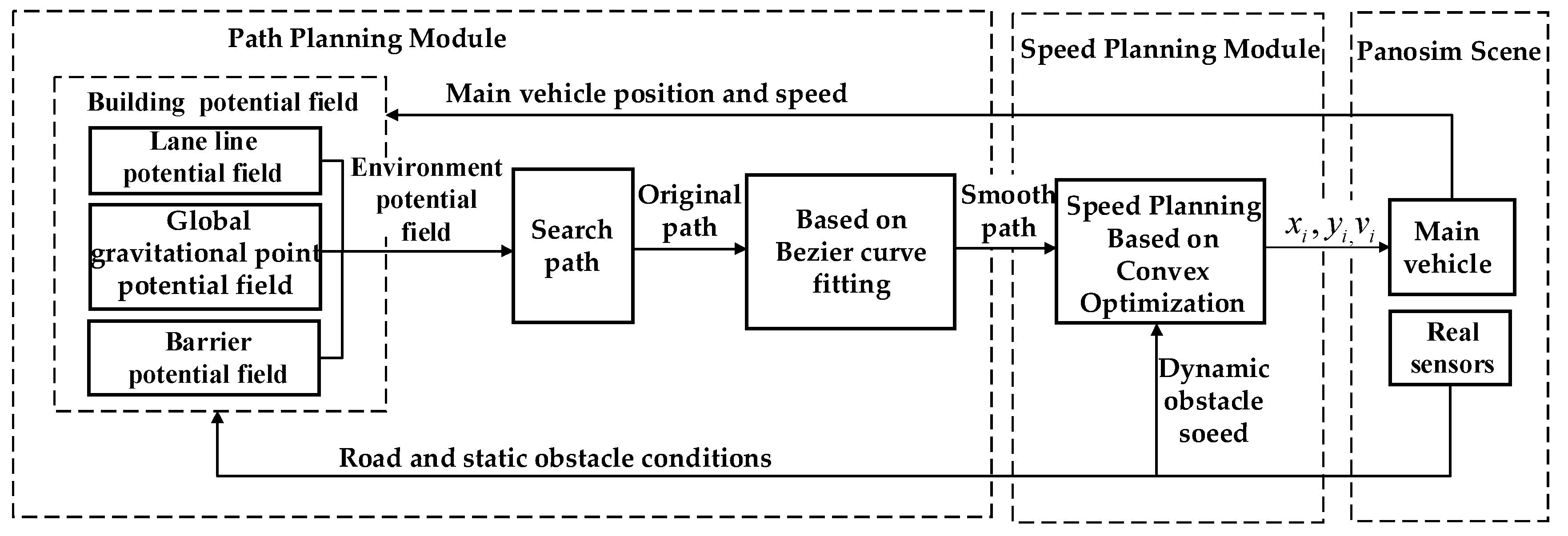
1. Introduction
2. Improvement of the Artificial Potential Field Method
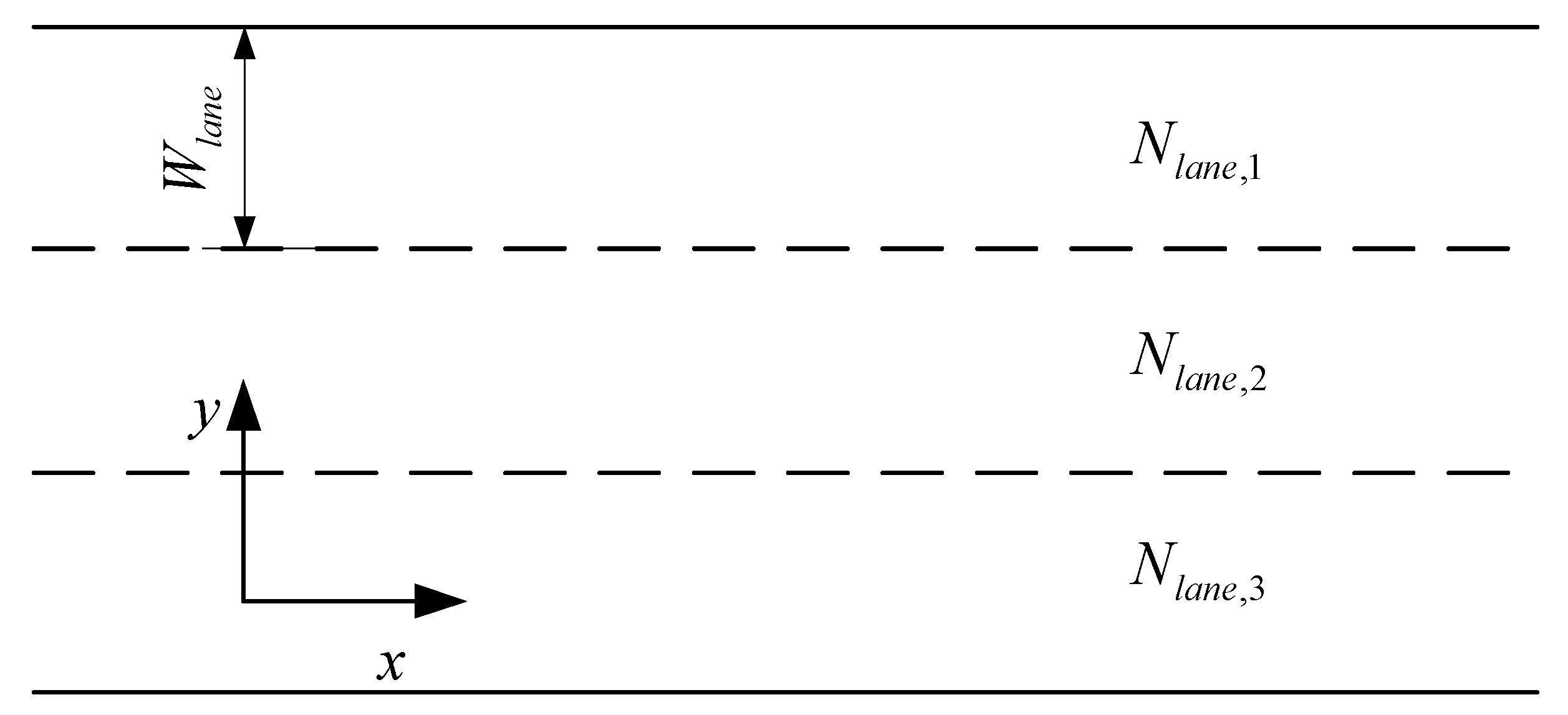
2.1. Road Boundary Repulsive Force Field
2.2. Gravitational Potential Field
2.3. Obstacle-Repulsive Potential Field
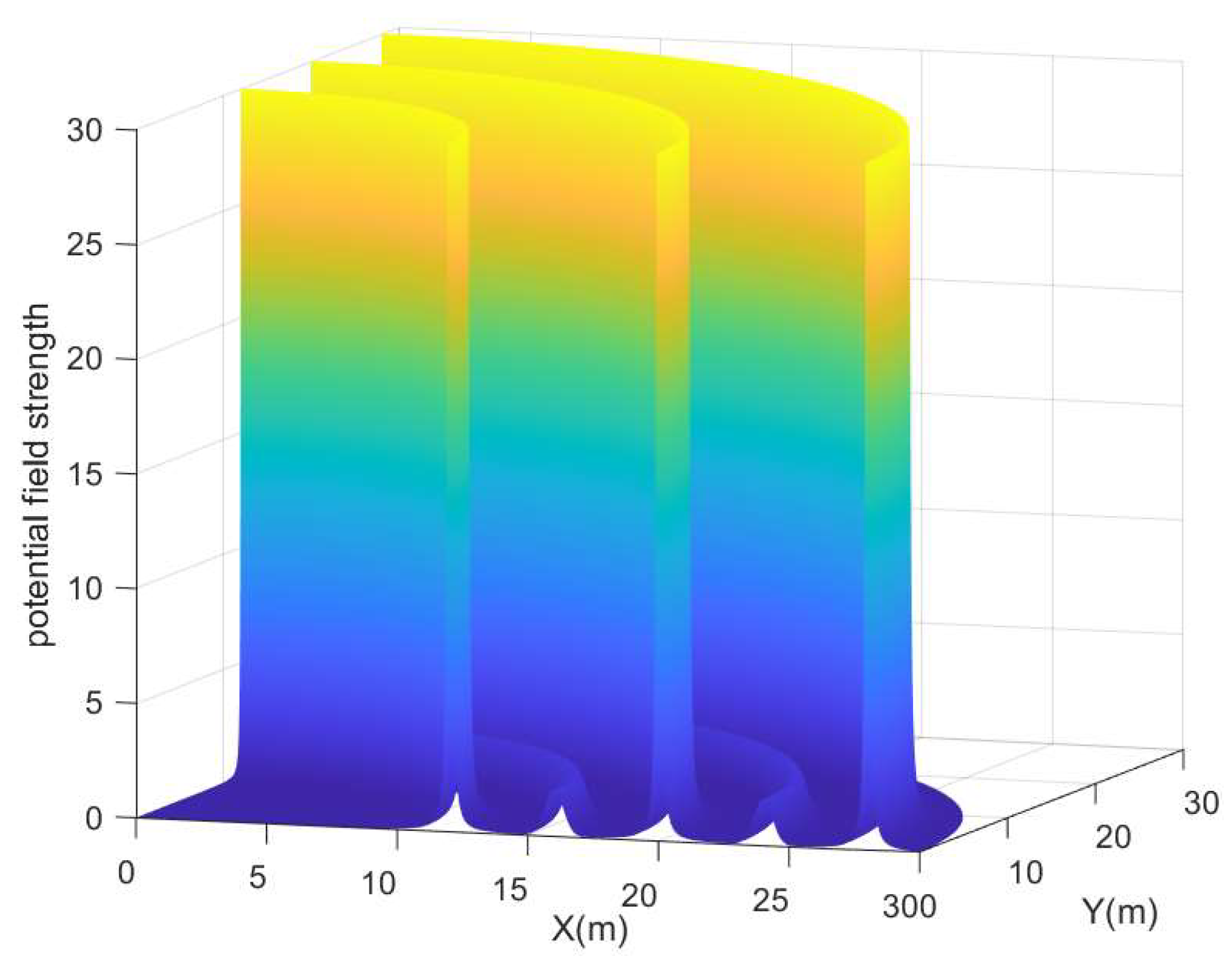
2.3.1. Potential Field Model
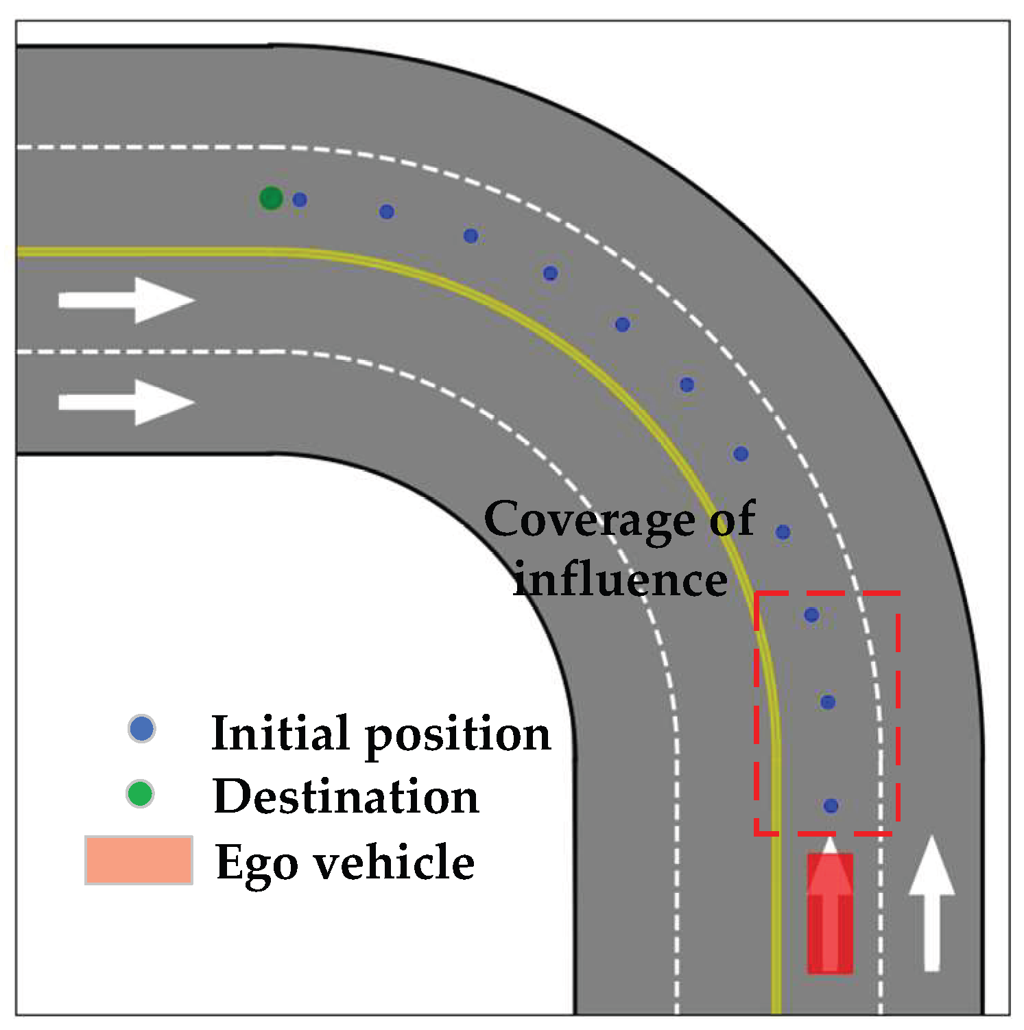
2.3.2. Range of Repulsive Force Field
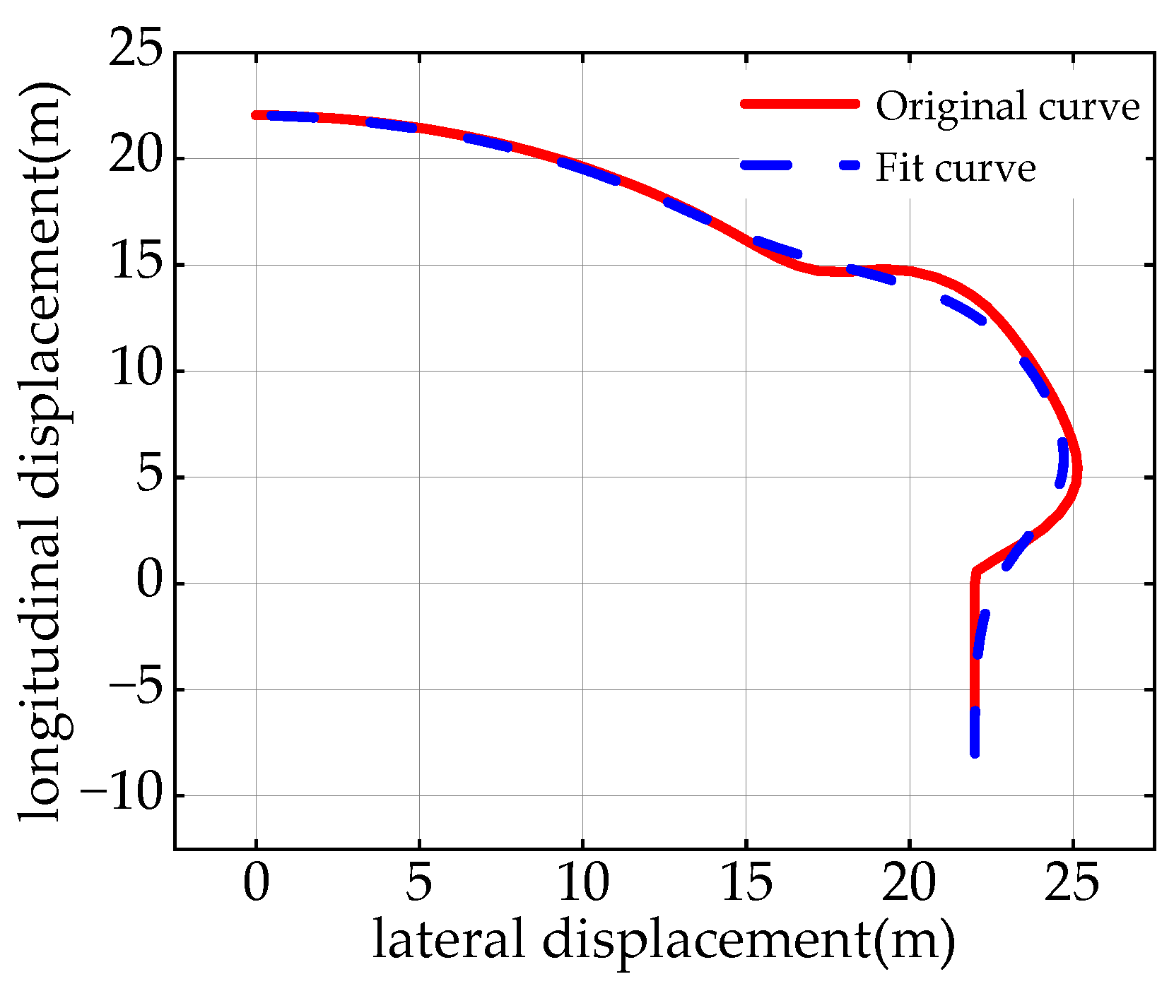
2.4. Bezier Curves Fitting
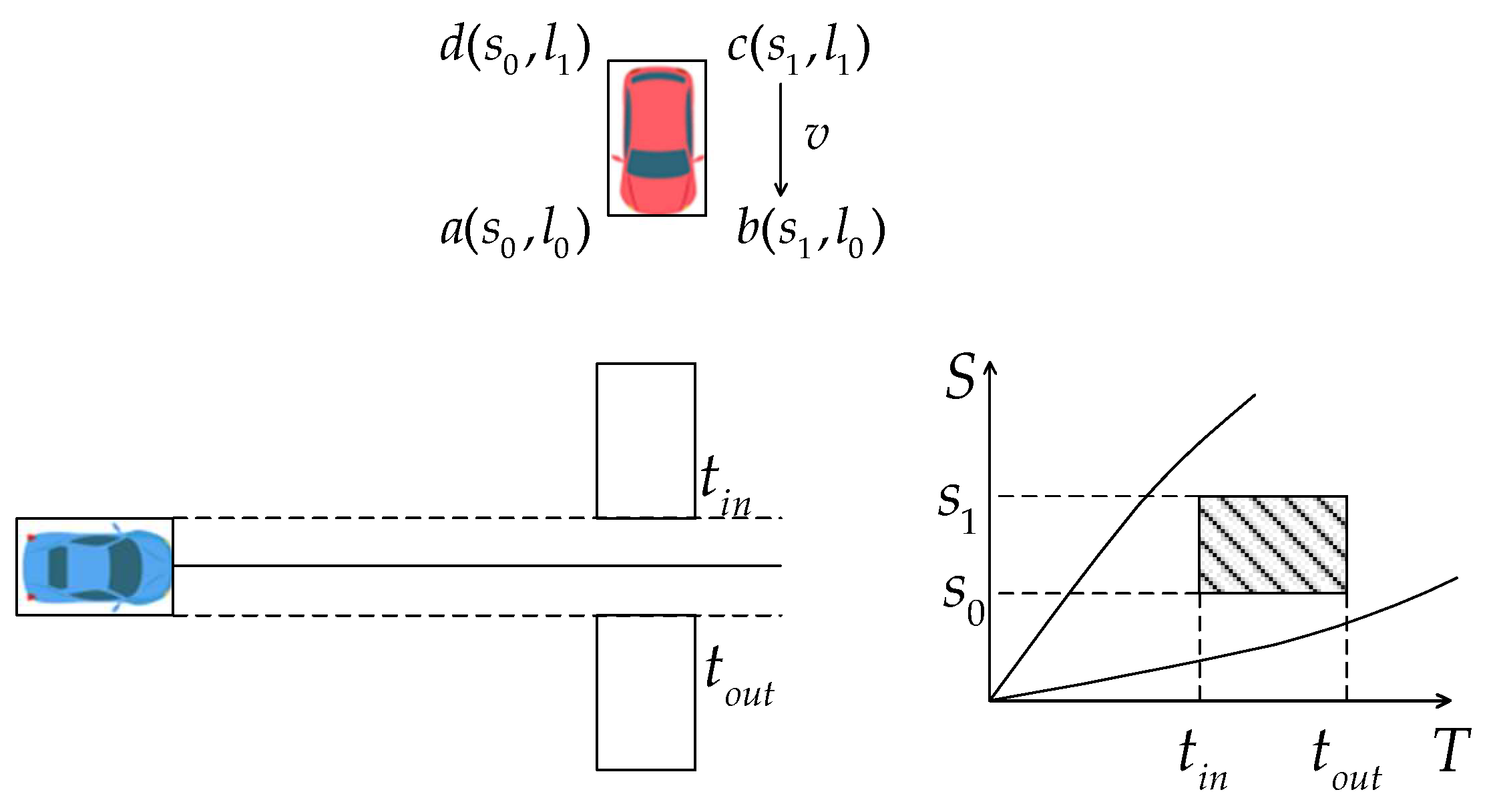
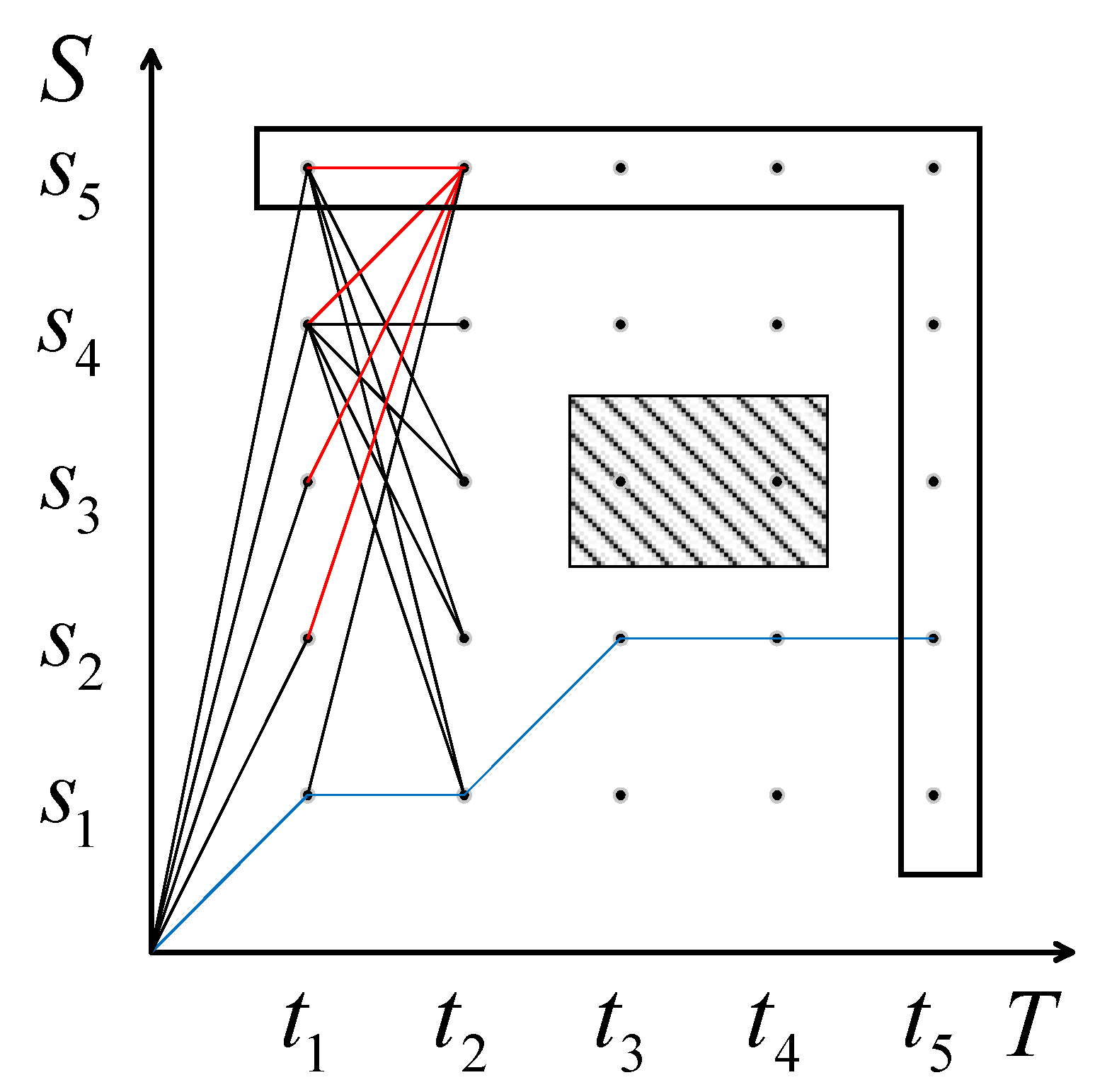
3. Speed Planning Based on the S-T Graph
3.1. Dynamic Planning
- (1)
- Obstacle Distance Cost Function
- (2)
- Recommended Speed Cost Function
- (3)
- Acceleration Cost Function
- (4)
- The Jerk Cost Function
3.2. Quadratic Planning
3.2.1. Establishing the Cost Function
- (1)
- The Cost of Speed
- (2)
- The Cost of Acceleration
- (3)
- The Cost of Jerk
3.2.2. Constraint Condition
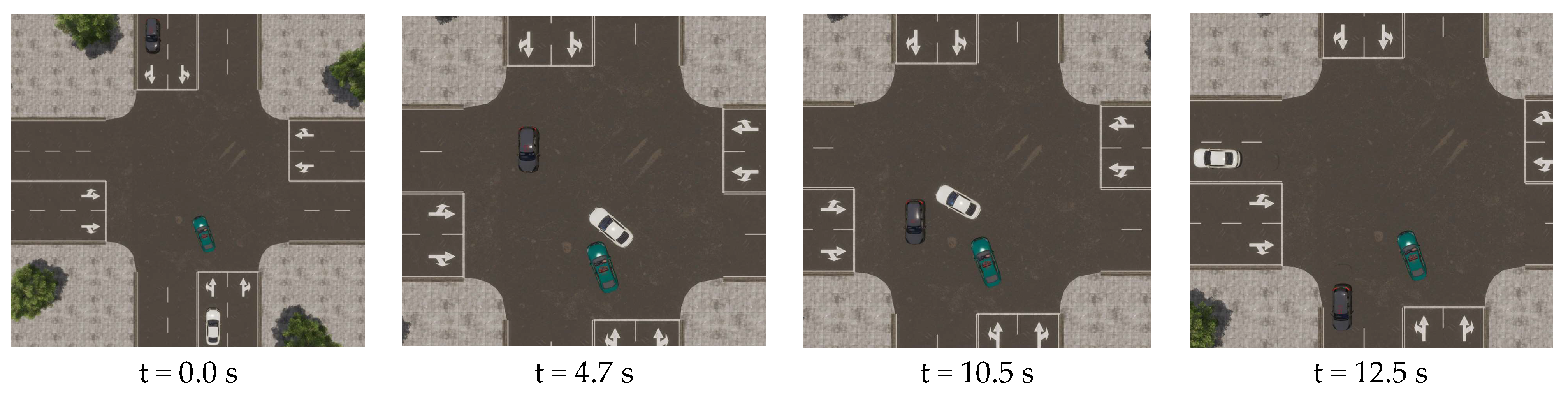
4. Simulation Verification
4.1. Description of the Simulation
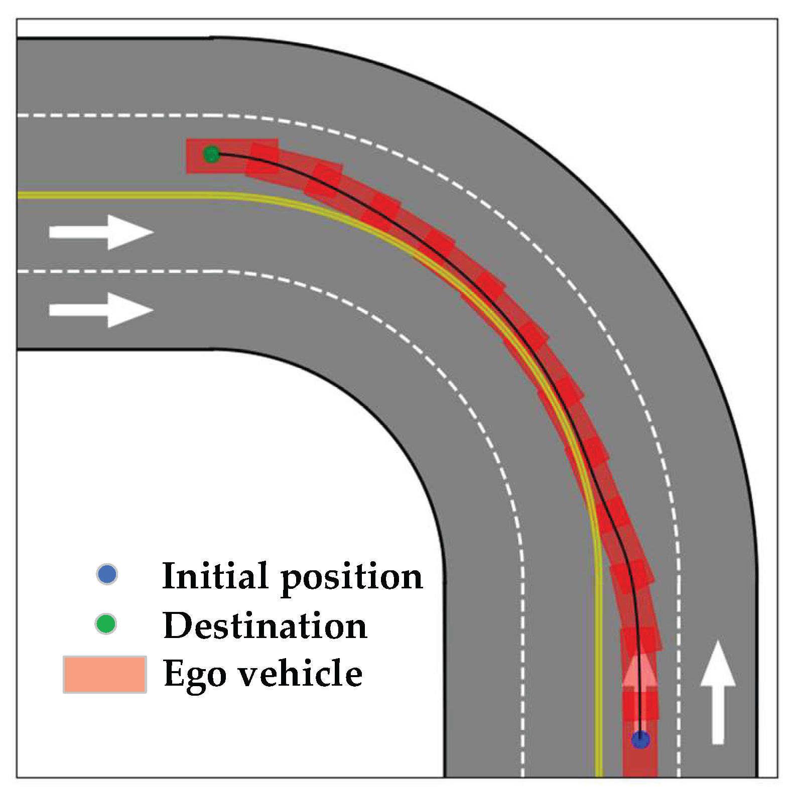
4.2. Path Planning
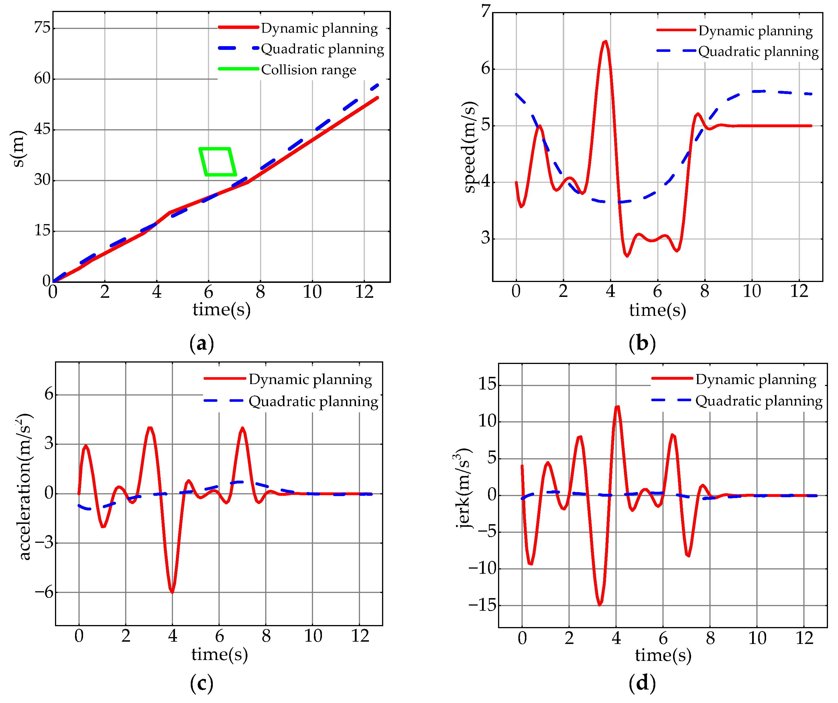
4.3. Speed Planning
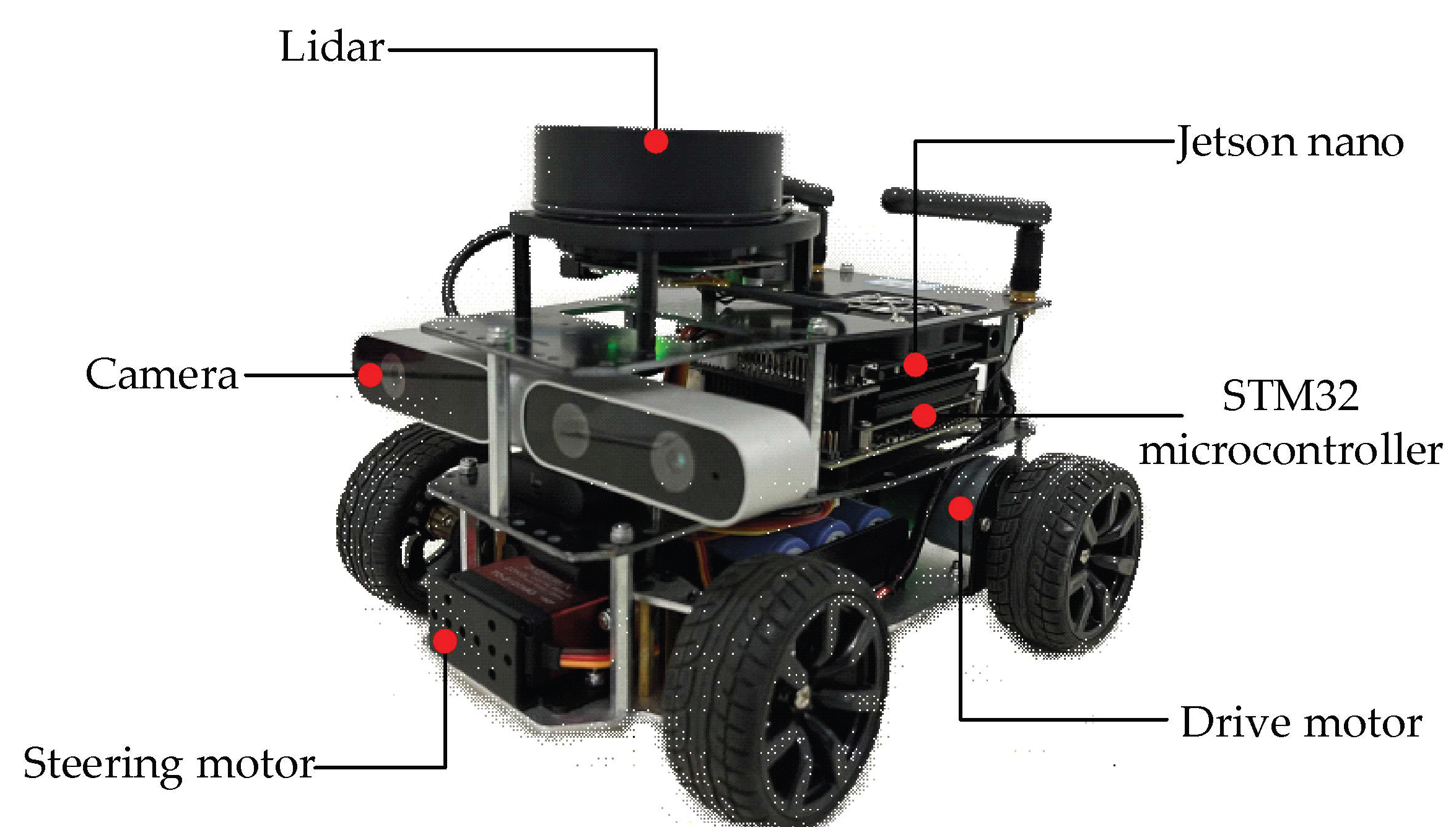
5. Experimental Verification
5.1. Experimental Condition
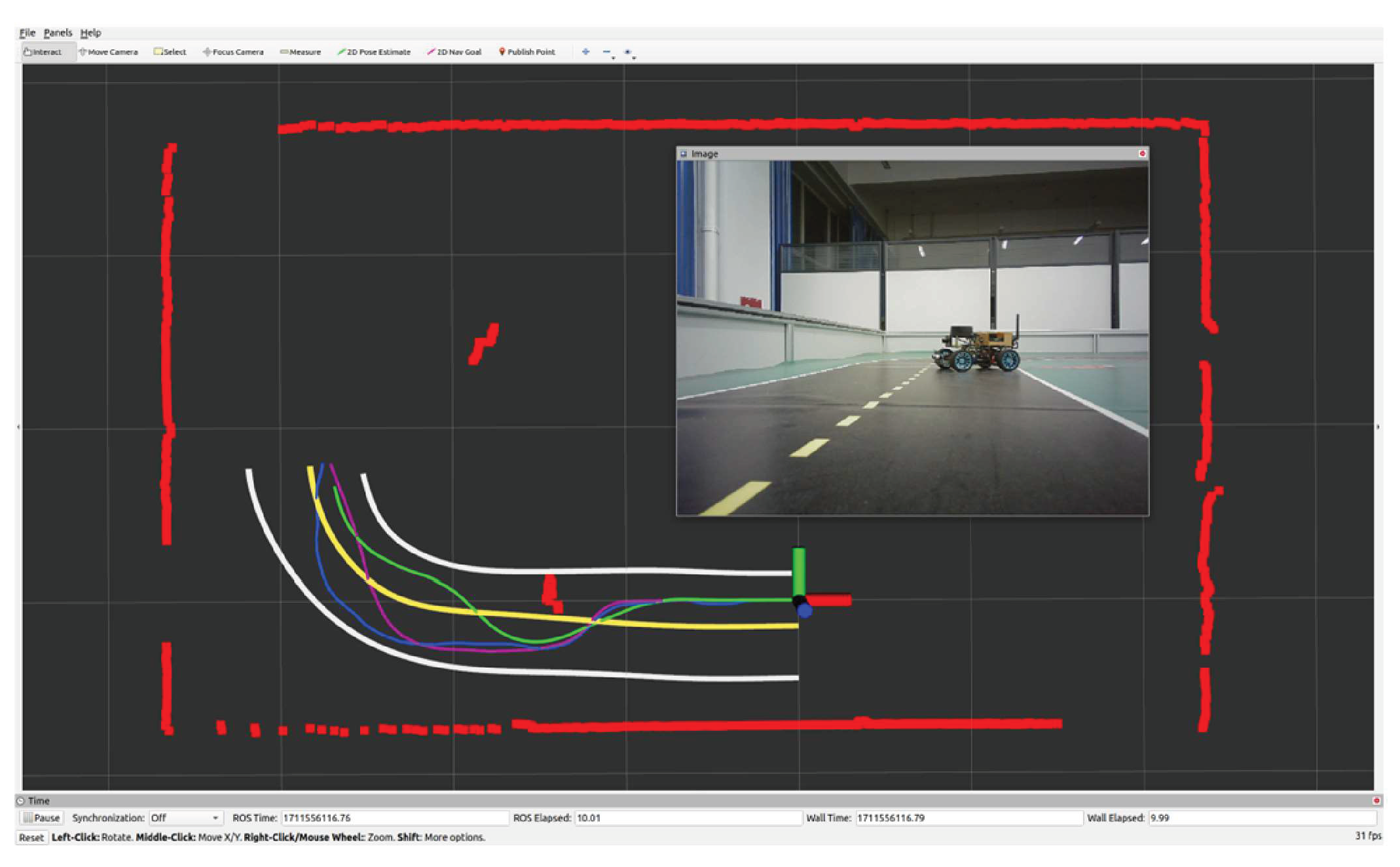
5.2. Experimental Results
5.3. Analysis of Results
6. Conclusions
Author Contributions
Funding
Data Availability Statement
Conflicts of Interest
References
- Zhang, Y.; Chen, H.; Waslander, S.L.; Gong, J.; Xiong, G.; Yang, T.; Liu, K. Hybrid trajectory planning for autonomous driving in highly constrained environments. IEEE Access 2018, 6, 32800–32819. [Google Scholar] [CrossRef]
- Zhu, D.-D.; Sun, J.-Q. A new algorithm based on Dijkstra for vehicle path planning considering intersection attribute. IEEE Access 2021, 9, 19761–19775. [Google Scholar] [CrossRef]
- Li, X.; Sun, Z.; Cao, D.; He, Z.; Zhu, Q. Real-time trajectory planning for autonomous urban driving: Framework, algorithms, and verifications. IEEE/ASME Trans. Mechatron. 2015, 21, 740–753. [Google Scholar] [CrossRef]
- Kavraki, L.E.; Kolountzakis, M.N.; Latombe, J.-C. Analysis of probabilistic roadmaps for path planning. IEEE Trans. Robot. Autom. 1998, 14, 166–171. [Google Scholar] [CrossRef]
- Kavraki, L.E.; Svestka, P.; Latombe, J.-C.; Overmars, M.H. Probabilistic roadmaps for path planning in high-dimensional configuration spaces. IEEE Trans. Robot. Autom. 1996, 12, 566–580. [Google Scholar] [CrossRef]
- Karaman, S.; Frazzoli, E. Sampling-based algorithms for optimal motion planning. Int. J. Robot. Res. 2011, 30, 846–894. [Google Scholar] [CrossRef]
- LaValle, S.M.; Kuffner, J.J., Jr. Randomized kinodynamic planning. Int. J. Robot. Res. 2001, 20, 378–400. [Google Scholar] [CrossRef]
- Khatib, O. Real-time obstacle avoidance for manipulators and mobile robots. Int. J. Robot. Res. 1986, 5, 90–98. [Google Scholar] [CrossRef]
- Duan, Y.; Yang, C.; Zhu, J.; Meng, Y.; Liu, X. Active obstacle avoidance method of autonomous vehicle based on improved artificial potential field. Int. J. Adv. Robot. Syst. 2022, 19, 17298806221115984. [Google Scholar] [CrossRef]
- Park, G.; Choi, M. Optimal Path Planning for Autonomous Vehicles Using Artificial Potential Field Algorithm. Int. J. Automot. Technol. 2023, 24, 1259–1267. [Google Scholar] [CrossRef]
- Yuan, C.; Weng, S.; Shen, J.; Chen, L.; He, Y.; Wang, T. Research on active collision avoidance algorithm for intelligent vehicle based on improved artificial potential field model. Int. J. Adv. Robot. Syst. 2020, 17, 1729881420911232. [Google Scholar] [CrossRef]
- Fan, X.; Guo, Y.; Liu, H.; Wei, B.; Lyu, W. Improved artificial potential field method applied for AUV path planning. Math. Probl. Eng. 2020, 2020, 6523158. [Google Scholar] [CrossRef]
- Tian, J.; Bei, S.; Li, B.; Hu, H.; Quan, Z.; Zhou, D.; Zhou, X.; Tang, H. Research on active obstacle avoidance of intelligent vehicles based on improved artificial potential field method. World Electr. Veh. J. 2022, 13, 97. [Google Scholar] [CrossRef]
- Santos, S.D.; Azinheira, J.R.; Botto, M.A.; Valério, D. Path planning and guidance laws of a formula student driverless car. World Electr. Veh. J. 2022, 13, 100. [Google Scholar] [CrossRef]
- Bevan, G.P.; Gollee, H.; O’reilly, J. Trajectory generation for road vehicle obstacle avoidance using convex optimization. Proc. Inst. Mech. Eng. Part D J. Automob. Eng. 2010, 224, 455–473. [Google Scholar] [CrossRef]
- Wiseman, Y. Autonomous Vehicles. In Encyclopedia of Information Science and Technology, 5th ed.; Khosrow-Pour, M., Ed.; IGI Global: Hershey, PA, USA, 2021; Volume 1, pp. 1–11. [Google Scholar] [CrossRef]
- Feng, S.; Qian, Y.; Wang, Y. Collision avoidance method of autonomous vehicle based on improved artificial potential field algorithm. Proc. Inst. Mech. Eng. Part D J. Automob. Eng. 2021, 235, 3416–3430. [Google Scholar] [CrossRef]
- Duraklı, Z.; Nabiyev, V. A new approach based on Bezier curves to solve path planning problems for mobile robots. J. Comput. Sci. 2022, 58, 101540. [Google Scholar] [CrossRef]
- Li, B.; Ouyang, Y.; Li, L.; Zhang, Y. Autonomous driving on curvy roads without reliance on frenet frame: A cartesian-based trajectory planning method. IEEE Trans. Intell. Transp. Syst. 2022, 23, 15729–15741. [Google Scholar] [CrossRef]
- Wang, P.; Liu, Y.; Yao, W.; Yu, Y. Improved A-star algorithm based on multivariate fusion heuristic function for autonomous driving path planning. Proc. Inst. Mech. Eng. Part D J. Automob. Eng. 2023, 237, 1527–1542. [Google Scholar] [CrossRef]
- Zhang, X.; Zhu, T.; Du, L.; Hu, Y.; Liu, H. Local path planning of autonomous vehicle based on an improved heuristic bi-rrt algorithm in dynamic obstacle avoidance environment. Sensors 2022, 22, 7968. [Google Scholar] [CrossRef] [PubMed]


| Parameters | Value | Parameters | Value |
|---|---|---|---|
| 10 | · (m) | 2 | |
| 0.35 | · (m) | 3.3 | |
| 0.5 | 1000 | ||
| 3 | · (m) | 0.5 | |
| 2 | · (m) | 1.5 | |
| 1.5 | 235 | ||
| 1.5 | 10 | ||
| 4.9 | 500 |
| C-APF | E-APF | DE-APF | |
|---|---|---|---|
| Fall into local optimality * | N | Y | N |
| Maximum longitudinal safety distance/m | 6.1211 | \ | 8.4459 |
| Maximum lateral safety distance/m | 4.9507 | \ | 4.4117 |
| Average curvature | 0.0709 | \ | 0.0652 |
| Maximum curvature | 0.2020 | \ | 0.1630 |
Disclaimer/Publisher’s Note: The statements, opinions and data contained in all publications are solely those of the individual author(s) and contributor(s) and not of MDPI and/or the editor(s). MDPI and/or the editor(s) disclaim responsibility for any injury to people or property resulting from any ideas, methods, instructions or products referred to in the content. |
© 2024 by the authors. Licensee MDPI, Basel, Switzerland. This article is an open access article distributed under the terms and conditions of the Creative Commons Attribution (CC BY) license (https://creativecommons.org/licenses/by/4.0/).
Share and Cite
Li, Y.; Li, G.; Peng, K. Research on Obstacle Avoidance Trajectory Planning for Autonomous Vehicles on Structured Roads. World Electr. Veh. J. 2024, 15, 168. https://doi.org/10.3390/wevj15040168
Li Y, Li G, Peng K. Research on Obstacle Avoidance Trajectory Planning for Autonomous Vehicles on Structured Roads. World Electric Vehicle Journal. 2024; 15(4):168. https://doi.org/10.3390/wevj15040168
Chicago/Turabian StyleLi, Yunlong, Gang Li, and Kang Peng. 2024. "Research on Obstacle Avoidance Trajectory Planning for Autonomous Vehicles on Structured Roads" World Electric Vehicle Journal 15, no. 4: 168. https://doi.org/10.3390/wevj15040168
APA StyleLi, Y., Li, G., & Peng, K. (2024). Research on Obstacle Avoidance Trajectory Planning for Autonomous Vehicles on Structured Roads. World Electric Vehicle Journal, 15(4), 168. https://doi.org/10.3390/wevj15040168