
Evaluation of Vehicle Lateral and Longitudinal Dynamic Behavior of the New Package-Saving Multi-Link Torsion Axle (MLTA) for BEVs


Abstract
1. Introduction
1.1. State of the Art
1.2. The Concept of the Novel Multi-Link Torsion Axle
1.3. Research Subject
2. Design, Modeling, and Full-Vehicle Integration of the MLTA
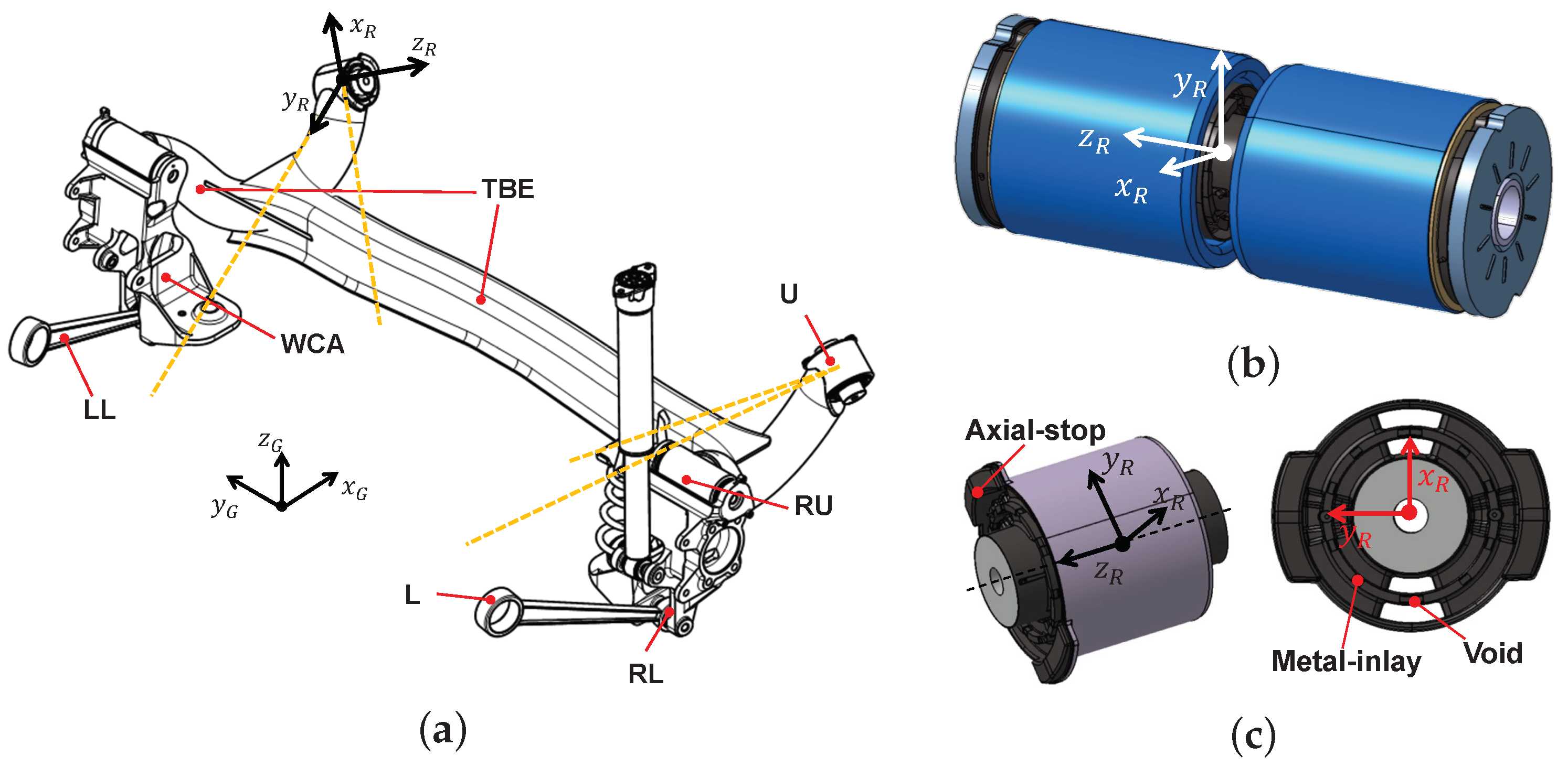
2.1. Compliance Analysis and Bushing Design
- -
- LC 1 (right cornering): in y-direction at wheel patch (WP)
- -
- LC 2 (obstacle crossing): in x-direction at wheel center (WC)
- -
- LC 3 (braking): in x-direction at wheel patch (WP)
2.2. Suspension Design and Manufacturing
2.2.1. Prototype Bushings
2.2.2. Component Design
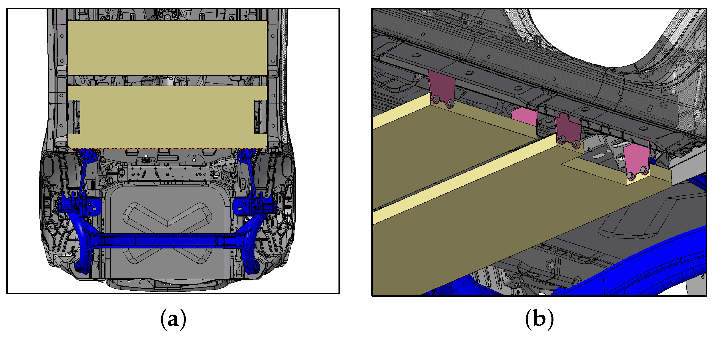
2.3. Full Vehicle—Design of the Battery Equivalent and Mass Properties
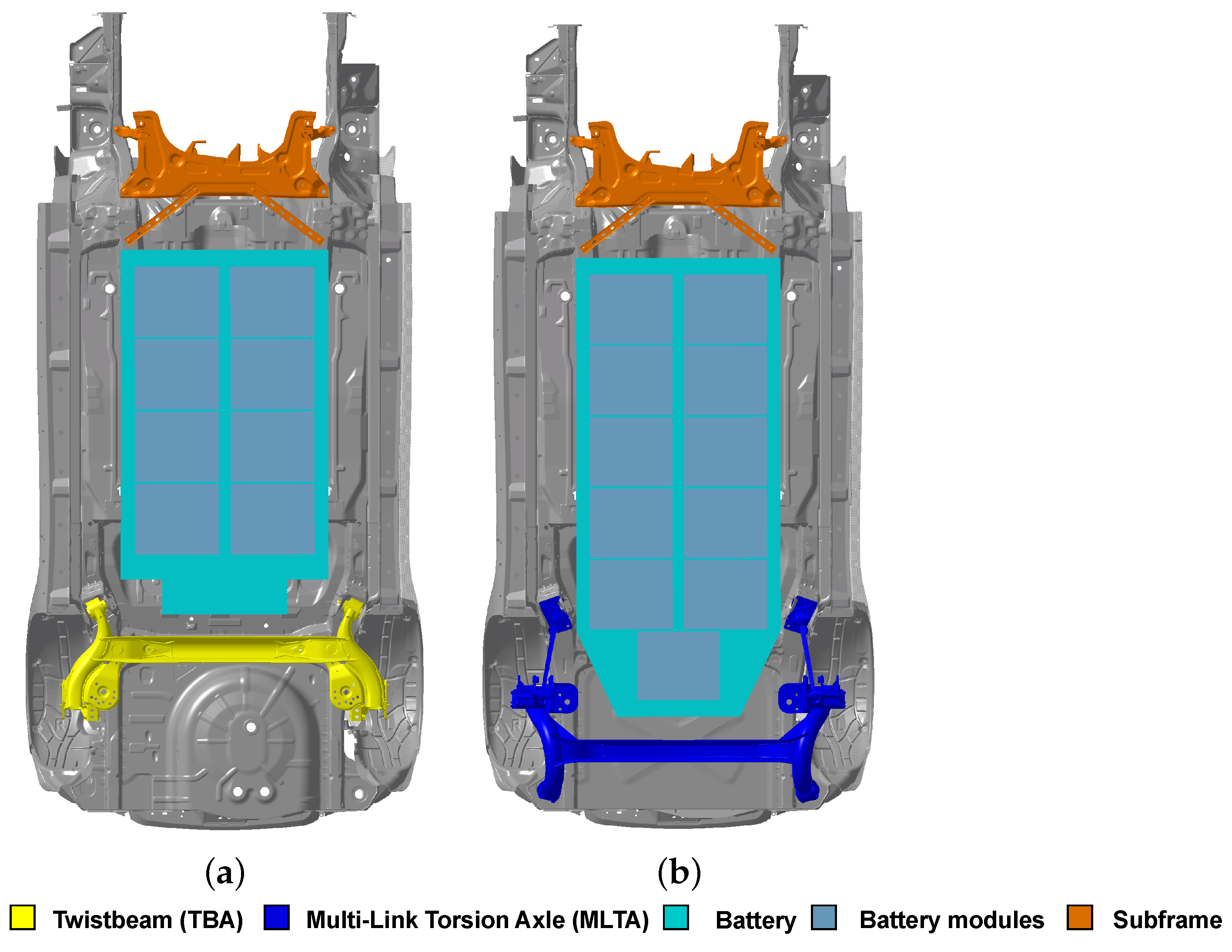
2.3.1. Vehicle Variants
2.3.2. Mass Dummy Development
3. Objective Evaluation of the MLTA
3.1. Testing the Component-Level Kinematics and Compliance
3.2. Testing at Vehicle Level—Objective Evaluation
3.2.1. Vehicle Instrumentation
3.2.2. Steady-State Evaluations—Constant-Radius Cornering
3.2.3. Steady-State Evaluations—Braking
3.2.4. Lateral Transient Response—Frequency Response with Sweep Steer Maneuver

| Characteristic Values | Figure | VarA | VarB | VarC | C to B |
|---|---|---|---|---|---|
| Constant-radius cornering (CRC) | |||||
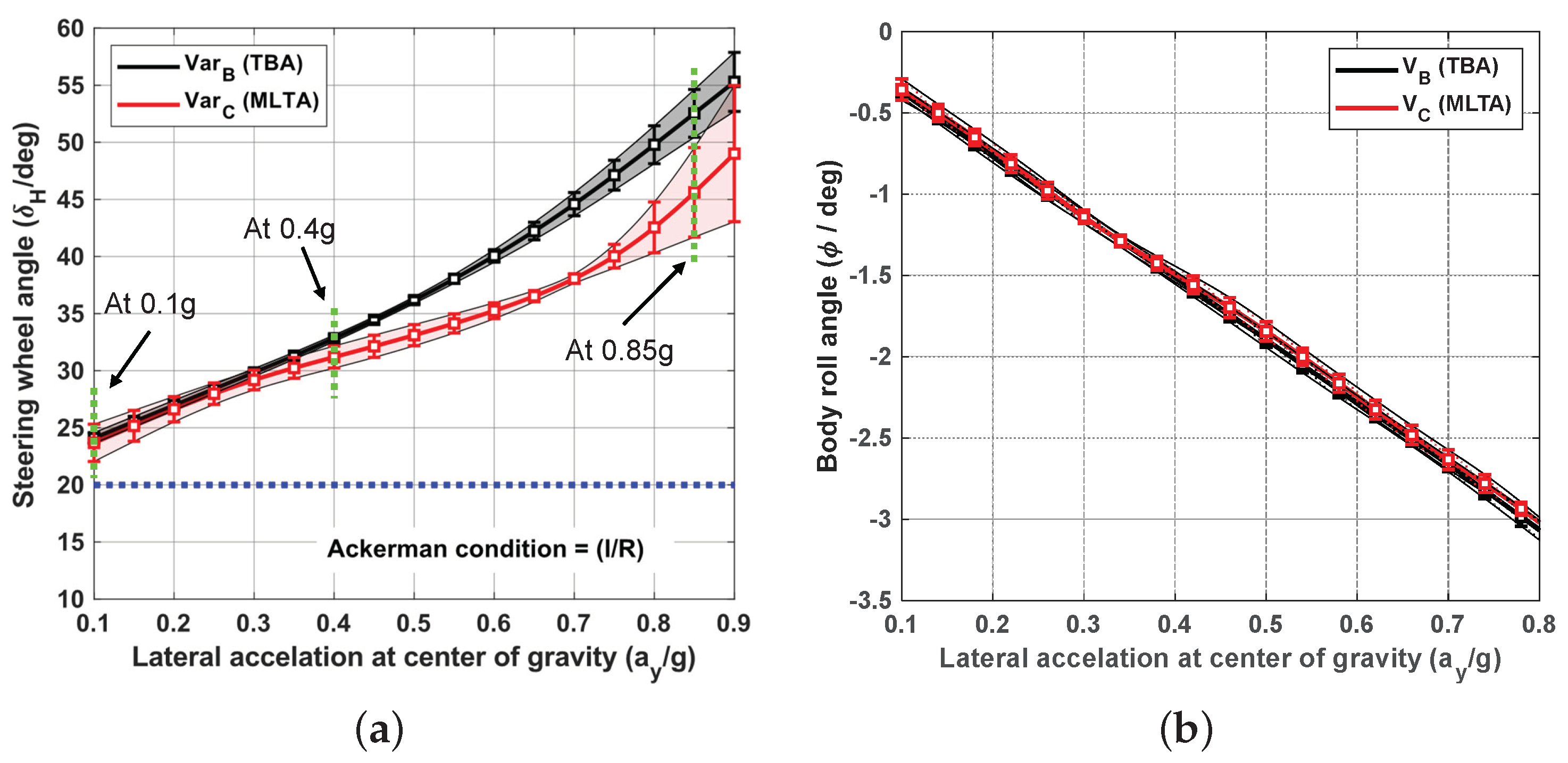
| ()0.1 Self-steering gradient @ 0.1g (deg/g) | Figure 14a | 29.0 | 30.0 | +3.4% | |
| ()0.4 Self-steering gradient @ 0.4g (deg/g) | Figure 14a | 31.0 | 19.0 | −38.7% | |
| ()0.85 Self-steering gradient @ 0.85g (deg/g) | Figure 14a | 55.0 | 66.0 | +20.0% | |
| () Roll gradient (deg/g) | Figure 14b | −3.85 | −3.81 | −1.0% | |
| Straight-line braking (SLB) | |||||
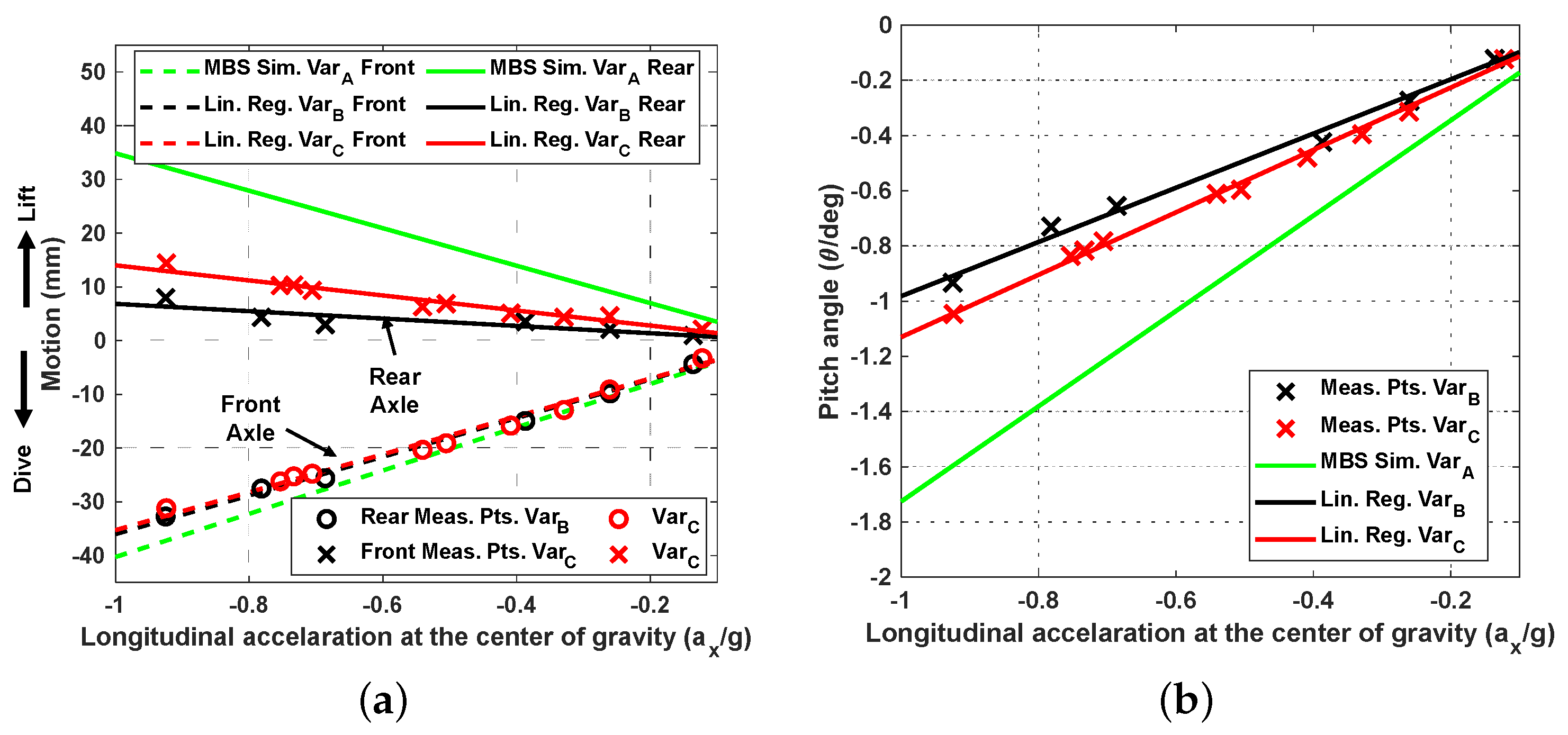
| Dive gradient (mm/g) | Figure 15a | 40.3 | 36.0 | 35.3 | −1.9% |
| Lift gradient (mm/g) | Figure 15a | −34.9 | −6.8 | −14.0 | −105.9% |
| Hip-point rise gradient (mm/g) | Figure 15a | −0.1 | 15.40 | 11.6 | −24.7% |
| Total pitch gradient (deg/g) | Figure 15b | 1.7 | 1.0 | 1.1 | 10% |
| Frequency response (FR) | |||||
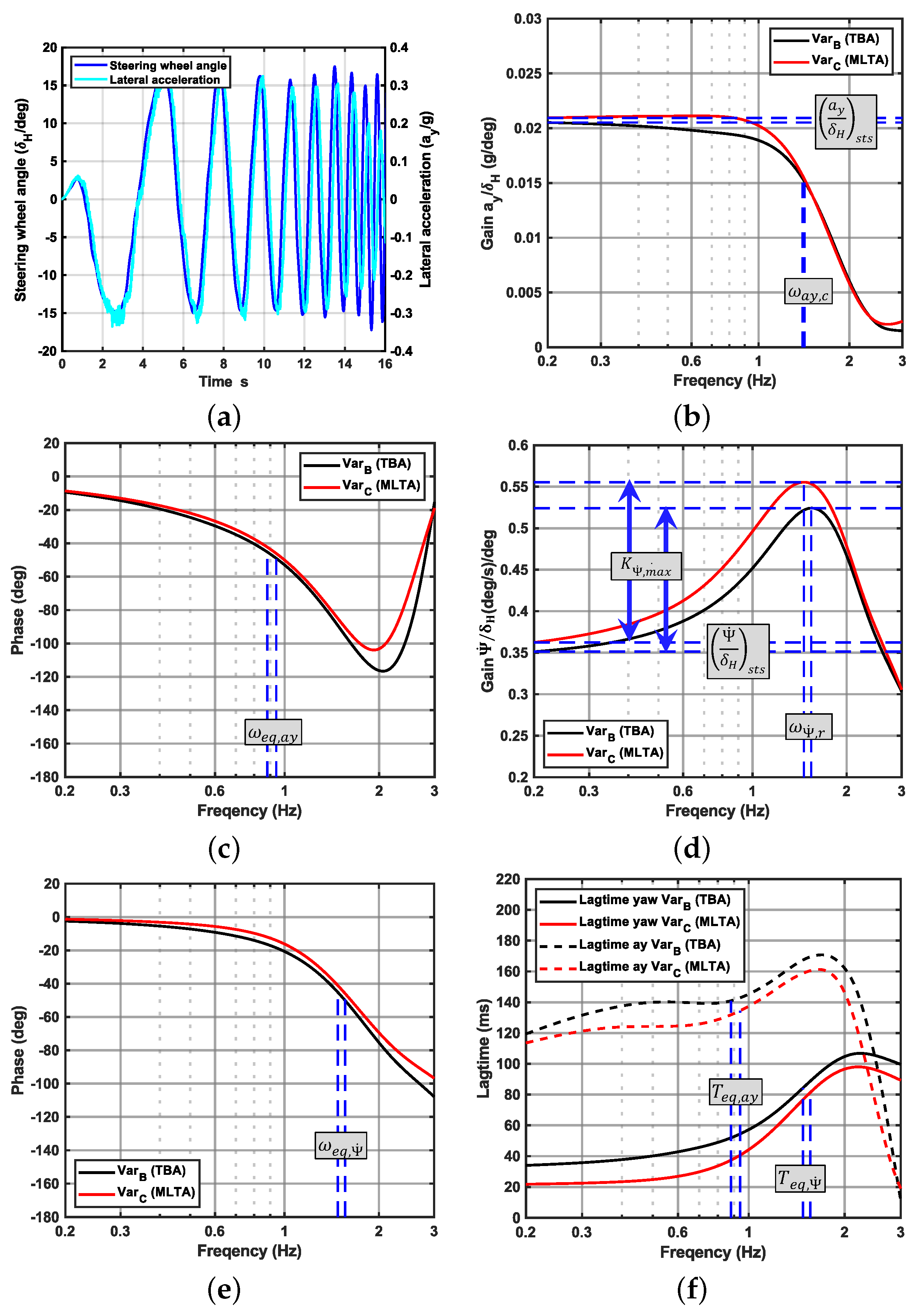
| Cut-off frequency (Hz) | Figure 16b | 1.42 | 1.4 | −1.4% | |
| Resonant frequency (Hz) | Figure 16d | 1.54 | 1.46 | −5.2% | |
| Gain for lateral acc. (g/deg) | Figure 16b | 2.05 | 2.09 | 2.1% | |
| Gain for yaw rate (deg/s)/deg | Figure 16d | 3.51 | 3.62 | 3.2% | |
| Gain ratio (−) | Figure 16d | 1.49 | 1.53 | 2.7% | |
| Effective time constant (ms) | Figure 16f | 141 | 135 | −4.6% | |
| Effective time constant (ms) | Figure 16f | 84 | 81 | −3.6% |
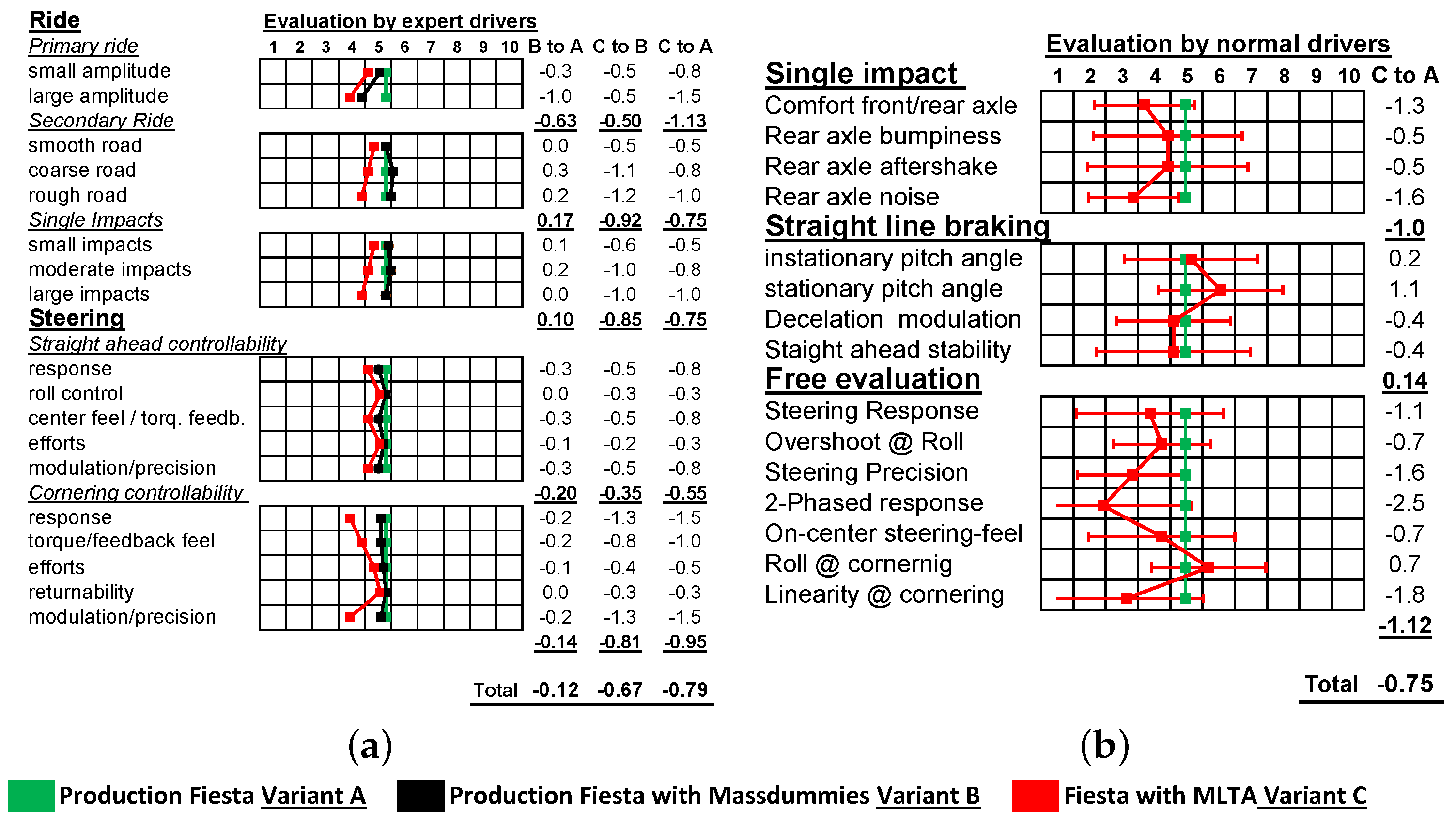
4. Subjective Evaluation of the MLTA Prototype
4.1. VarA to VarB Evaluation—Experts
4.2. VarA to VarC Evaluation—Experts
4.3. VarA to VarC Evaluation—Normal Drivers
5. Summary and Conclusions
- −
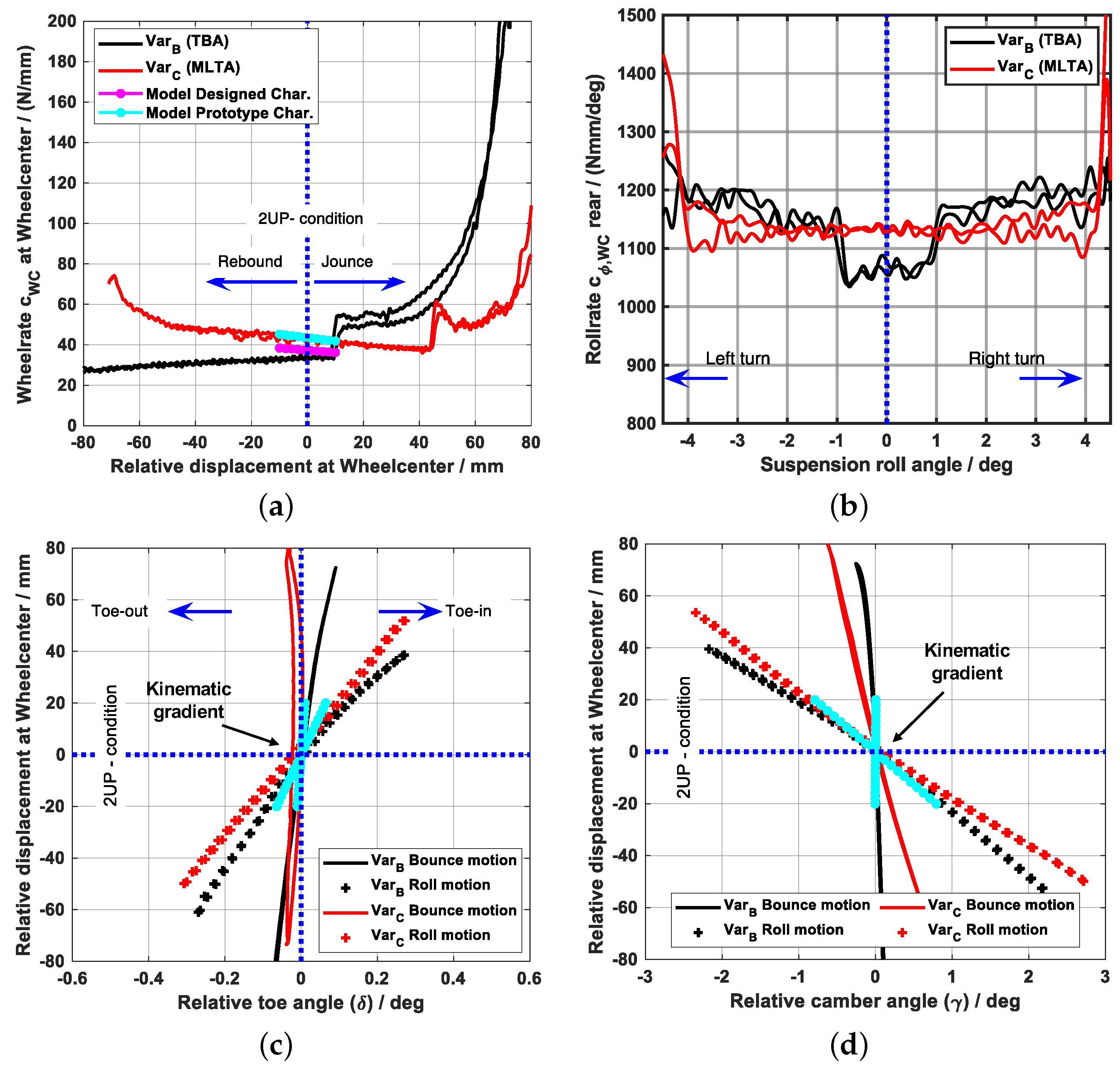
- The wheel rate was 30% higher and the camber compliance was 60% higher than VarB. Both deviations can be attributed to the tolerances in MLTA, especially the reduced stiffness of the elastomer bushings compared to the target stiffness values.
- −
- Together with the missing bump stop spacer for VarC, its wheel rate–wheel center displacement curves are different, as well as the roll rate–roll angle characteristics.
- −
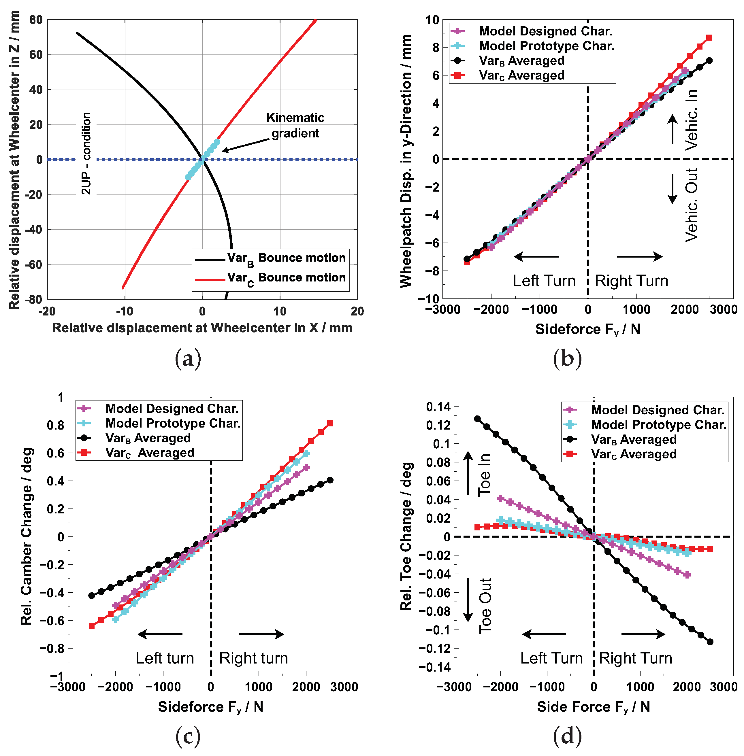
- The kinematic toe and camber gradients of MLTA are similar to VarB.
- −
- The wheel center recession characteristic was considerably improved, thus confirming the MLTA concept.
- −
- The constant-radius cornering tests show a reduced understeer of VarC compared with VarC that can be explained by the KnC findings.
- −
- In a straight-line braking maneuver, the MLTA (VarC) shows a 35% lower pitch gradient than VarA and a 10% higher gradient than VarB.
- −
- The results of the frequency response test based on a sweep steer input indicate an increased yaw gain and resonance peak. However, the lateral acceleration and yaw rate response times were reduced overall, leading to the conclusion that the MLTA vehicle should be more agile than VarB.
Author Contributions
Funding
Data Availability Statement
Acknowledgments
Conflicts of Interest
Glossary
| TBA | Twist-beam axle |
| BEV | Battery electric vehicle |
| KnC | Kinematic and compliance |
| MBS | Multibody simulation |
| MEB | Modular electric drive matrix |
| CLA | Composite leaf spring axle |
| MLTA | Multi-link torsion axle |
| MLA | Multi-link axle |
| OEM | Original equipment manufacturer |
| WCA | Wheel carrier |
| WP | Wheel patch |
| EEM | Elastic equivalent mechanism |
| DOF | Degree of freedom |
| PWT | Parallel wheel travel |
| OWT | Opposite wheel travel |
| WC | Wheel center |
| BC | Boundary condition |
| TBE | Twist-beam equivalent |
| LL | Longitudinal link |
| SC | Shear center |
| WN | Wheel normal |
| BIW | Body in white |
| U | Upper body mount |
| L | Lower body mount |
| RU | Upper wheel carrier point middle |
| RUi | Upper wheel carrier point inner |
| RUo | Upper wheel carrier point outer |
| RL | Lower wheel carrier point |
| G | Global coordinate system |
| IC | Instantaneous center of motion |
| VarA | Variant A |
| VarB | Variant B |
| VarC | Variant C |
| ICE | Internal combustion engine |
| IMU | Inertia measurement unit |
| CRC | Constant-radius cornering |
| FFT | Fast Fourier transformation |
| PSD | Power spectral density |
| Notation | Description | Unit |
| Braking force at the wheel patch | N | |
| Wheel load change caused by load transfer | N | |
| Resulting force vector at the wheel patch during braking | N | |
| Force that is counteracted via the suspension | N | |
| Force vertical direction at the wheel patch that needs to be counteracted via the spring | N | |
| Spring force at the wheel carrier (spring attachment) | N | |
| Kinematic spring ratio between spring position and the wheel patch | – | |
| Ideal brake support angle | deg | |
| Brake support angle resulting from the suspension geometry | deg | |
| Unit vector oriented in the spring direction | mm | |
| Anti-lift ratio at the rear axle | % | |
| Dive gradient at the front axle | deg/mm | |
| Lift gradient at the rear axle | deg/mm | |
| Pitch angle of the vehicle | deg | |
| Pitch angle gradient | deg/g | |
| Body roll angle of the vehicle | deg | |
| Roll angle gradient | deg/g | |
| DOF rotation axis for parallel wheel travel | – | |
| DOF rotation axis for opposite wheel travel | – | |
| First Euler rotation angle around the z-axis (Z-X’-Z”) convention | deg | |
| Second Euler rotation angle around the -axis (Z-X’-Z”) convention | deg | |
| Third Euler rotation angle around the -axis (Z-X’-Z”) convention | deg | |
| Mass of the battery pack | kg | |
| Mass of the internal combustion engine | kg | |
| Mass of the fuel tank | kg | |
| Overall mass of the mass dummies | kg | |
| Overall mass of the vehicle | kg | |
| Front axle load | kg | |
| Rear axle load | kg | |
| Center of gravity | mm | |
| Inertia tensor | kg·mm2 | |
| 12x12 Compliance matrix to represent the TBE structure | ||
| Coefficient matrix for reaction force calculation | ||
| Coefficient matrix for deformation velocity calculation | ||
| Constant vector for reaction force calculation | ||
| Constant vector for deformation velocity calculation | ||
| Global reaction force and moment vector | ||
| Input force corresponding to the different load cases | ||
| Velocity vector for the multibody system caused by elastic deformation velocity | ||
| Wheel rate: force gradient in vertical direction at the wheel center during bounce motion | N/mm | |
| Roll rate: moment gradient in vertical direction at the wheel center during roll motion | N·mm/deg | |
| Camber compliance | deg/kN | |
| Toe compliance | deg/kN | |
| Lateral compliance at the wheel patch position | mm/kN | |
| Camber gradient: camber angle change during roll motion | deg/mm | |
| Toe gradient: toe angle change during roll motion | deg/mm | |
| Static toe angle | deg | |
| Static camber angle | deg | |
| Wheel center recession: ratio longitudinal to vertical wheel center motion | mm/m | |
| Steering wheel angle | deg | |
| Longitudinal acceleration at the center of gravity | g | |
| Lateral acceleration at the center of gravity | g | |
| Self-steering gradient | deg/g | |
| Side slip angle at the driver’s hip point | deg | |
| Side slip angle gradient at the driver’s hip point | deg/deg | |
| R | Cornering radius | m |
| l | Vehicle length: front wheel center to rear wheel center | m |
| Vehicle side slip angle at the rear | deg | |
| Vehicle side slip angle at the front | deg | |
| Distance from the correvit sensor to the front wheel center | m | |
| Velocity vector measured from the correvit sensor | m/s | |
| Yaw rate measured from the IMU | deg/s | |
| Cornering stiffness at the front | N/deg | |
| Cornering stiffness at the rear | N/deg | |
| Cut-off frequency: reduction in the signal power, -3dB | Hz | |
| Resonant frequency of the yaw rate | Hz | |
| Steady-state gain of the yaw rate | (deg/s)/deg | |
| Steady-state gain of the lateral acceleration | g/deg | |
| Peak-to-gain ratio | ||
| Effective time constant: lag time at phase angle | ms | |
| Signal x in the time domain | ||
| Signal x in the frequency domain | ||
| Conjugate complex signal x in the frequency domain | ||
| Auto-power spectrum | ||
| Cross-power spectrum | ||
| Bandwidth of the frequency bin (frequency resolution of the FFT) | Hz | |
| Sample rate of the time signal | Hz | |
| N | Number of discrete FFT points | |
| Complex transfer function |
References
- European Commission. Fit for 55: Delivering the EU’s 2030 Climate Target on the Way to Climate Neutrality; European Commission: Brussels, Belgium, 2021. [Google Scholar]
- Kraftfahrt-Bundesamt. Fahrzeugzulassungen Im Dezember 2021—Jahresbilanz: Press Release Nr. 1/2022; Technical Report; Kraftfahrt-Bundesamt: Flensburg, Germany, 2022. [Google Scholar]
- Wilmes, M.; Kraaijeveld, R.; Schrage, M.; Schummers, F. Challenges and Solutions of Converting Conventional Vehicles to Hybrid Electric or Battery Electric Vehicles. In Proceedings of the 10th International Munich Chassis Symposium, Munich, Germany, 25–26 June 2019; Pfeffer, P.E., Ed.; Springer Fachmedien Wiesbaden: Wiesbaden, Germany, 2020; pp. 343–353. [Google Scholar] [CrossRef]
- Hacker, C.; Hofmann, P.; Krahn, S.; Lobo Casanova, I. Composite Leaf Spring Axle für Pkw: Glasfaserverstärkt. Lightweight Des. 2015, 8, 14–19. [Google Scholar] [CrossRef]
- Ditzer, B.; Rosta, S.; Koopmann, J. Leichtbau von Tragfedern für Plug-in-Hybrid- und Elektrofahrzeuge. Automobiltechnische Zeitschrift 2022, 124, 50–55. [Google Scholar] [CrossRef]
- Fang, X.F. Rear Suspension for Electric Vehicle and Vehicle Body. Patent CN105365543A, 2 March 2016. [Google Scholar]
- Niessing, T.; Fang, X.F. Kinematic Analysis and Optimisation of a Novel Multi-Link Torsion Axle. Mech. Mach. Theory 2021, 165, 104432. [Google Scholar] [CrossRef]
- Olschewski, J.; Fang, X.F. Elastokinematic design and optimization of the multi-link torsion axle—A novel rear axle concept for BEVs. Mech. Based Des. Struct. Mach. 2024, 1–32. [Google Scholar] [CrossRef]
- Fang, X.F.; Tan, K. Analytical Modelling of Twist Beam Axles. Int. J. Veh. Syst. Model. Test. 2018, 13, 1–25. [Google Scholar] [CrossRef]
- Seth, M.K.; Glorer, J.; Schellhaas, R. Design of A New Weight and Cost Efficient Torsion Profile for Twistbeam Suspension. In Proceedings of the WCX™17: SAE World Congress Experience, Detroit, MI, USA, 4–6 April 2017. [Google Scholar] [CrossRef]
- A2Mac1. 3D-Scan, Opel Ampera-e, 2018.
- Lu, Y.; Rong, X.; Hu, Y.S.; Chen, L.; Li, H. Research and Development of Advanced Battery Materials in China. Energy Storage Mater. 2019, 23, 144–153. [Google Scholar] [CrossRef]
- International Energy Agency. Global EV Outlook 2023: Catching Up with Climate Ambitions; Global EV Outlook; International Energy Agency: Paris, France, 2023. [Google Scholar] [CrossRef]
- Wang, C.; He, L.; Sun, H.; Zhu, J.; Lu, Z.; Zhu, Y.; Hu, S. A kind of Lithium Ion Battery, Battery Module, Battery Pack and Automobile. Chinese Patent CN110518156A, 29 November 2019. [Google Scholar]
- Sumpf; Pires, A.; Stockton, W.B.; Spooner, C.; Prodan, C.; Gorasia, J.B.; Harris, K.; Burke, D.; Szafer, D.G.; Patel, K.; et al. Integrated Energy Storage System. U.S. Patent WO2021102340A1, 27 May 2021. [Google Scholar]
- Wassiliadis, N.; Steinsträter, M.; Schreiber, M.; Rosner, P.; Nicoletti, L.; Schmid, F.; Ank, M.; Teichert, O.; Wildfeuer, L.; Schneider, J.; et al. Quantifying the State of the Art of Electric Powertrains in Battery Electric Vehicles: Range, Efficiency, and Lifetime from Component to System Level of the Volkswagen ID.3. eTransportation 2022, 12, 100167. [Google Scholar] [CrossRef]
- Matschinsky, W. Radführungen Der Straßenfahrzeuge, 3rd ed.; Springer: Berlin/Heidelberg, Germany, 2007. [Google Scholar]
- Tavernini, D.; Velenis, E.; Longo, S. Feedback Brake Distribution Control for Minimum Pitch. Veh. Syst. Dyn. 2017, 55, 902–923. [Google Scholar] [CrossRef]
- DIN ISO 7401; Straßenfahrzeuge: Testverfahren Für Querdynamisches Übertragungsverhalten. ISO: Geneva, Switzweland, 1989.
- Havelock, D.; Kuwano, S.; Vorländer, M. (Eds.) Handbook of Signal Processing in Acoustics, 1st ed.; Springer: New York, NY, USA, 2016. [Google Scholar]
- Decker, M. Zur Beurteilung Der Querdynamik von Personenkraftwagen. Ph.D. Thesis, Technische Universität München, Munich, Germany, 2009. [Google Scholar]
- Weir, D.H.; Dimarco, R.J. Correlation and Evaluation of Driver/Vehicle Directional Handling Data. In Proceedings of the 1978 Automotive Engineering Congress and Exposition, Detroit, MI, USA, 1 February 1978; p. 780010. [Google Scholar] [CrossRef]
- Chen, D.C.; Crolla, D.A. Subjective and Objective Measures of Vehicle Handling: Drivers & Experiments. Veh. Syst. Dyn. 1998, 29, 576–597. [Google Scholar] [CrossRef]
- Becker, K. (Ed.) Subjektive Fahreindrücke Sichtbar Machen IV: Korrelation Zwischen Objektiver Messung und Subjektiver Beurteilung in der Fahrzeugentwicklung; Number 4 in Subjektive Fahreindrücke Sichtbar Machen; Expert: Renningen, Germany, 2010. [Google Scholar]
- Schindler, E. Fahrdynamik: Grundlagen Des Lenkverhaltens Und Ihre Anwendung Für Fahrzeugregelsysteme, 3rd ed.; Expert: Tübingen, Germany, 2019. [Google Scholar]
- Mimuro, T.; Ohsaki, M.; Yasunaga, H.; Satoh, K. Four Parameter Evaluation Method of Lateral Transient Response. In Proceedings of the Passenger Car Conference & Exposition, Dearborn, MI, USA, 17–20 September 1990; p. 901734. [Google Scholar] [CrossRef]
- Barter, N.F. Analysis and Interpretation of Steady-State and Transient Vehicle Response Measurements. Veh. Syst. Dyn. 1976, 5, 79–103. [Google Scholar] [CrossRef]
- Mitschke, M.; Wallentowitz, H. Dynamik Der Kraftfahrzeuge, 5th ed.; Springer Vieweg: Wiesbaden, Germany, 2014. [Google Scholar]


| Right Cornering | Obstacle Crossing | Braking | |||||||
|---|---|---|---|---|---|---|---|---|---|
| LC1 | LC2 | LC 3 | |||||||
| X | Y | Z | X | Y | Z | X | Y | Z | |
| % | % | % | % | % | % | % | % | % | |
| U | 67 | −200 | 37 | −64 | 0 | 4 | 36 | 0 | −2 |
| RUi | −40 | −50 | −968 | −281 | 0 | −114 | −392 | −12 | −388 |
| RUo | 40 | −50 | 968 | 281 | 0 | 114 | 392 | −12 | 388 |
| WP | 0 | 0 | 22 | 0 | 0 | −19 | 0 | 0 | −55 |
| RL | 1 | 0 | 0 | −36 | 6 | 15 | −136 | 24 | 57 |
| L | 1 | 0 | 0 | −36 | 6 | 15 | −136 | 24 | 57 |
| LC1 | LC1 | LC1 | LC2 | LC3 | |
|---|---|---|---|---|---|
| RU | 0.15 | 1.20 | 0.10 | ||
| WC | 0.06 | 0.006 | 0.30 | ||
| TBE | 0.04 | 0.025 | 0.44 | 0.11 | |
| WP | 0.03 | 0.18 | 0.14 | ||
| L | 0.50 | ||||
| RL | < | 0.01 | |||
| U | 1.04 | 0.07 | |||
| SUM | 0.24 | 3.16 | 0.95 | ||
| TBA (reference) | 0.18 | 3.03 | 1.49 |
| Eulerangles | |||||||
|---|---|---|---|---|---|---|---|
| U (designed) | 100% | 100% | 100% | - | - | 100% | 348.7, 122.8, 114.7 |
| U (prototype) | 121% | 107% | 163% | - | - | 178% | 348.7, 122.8, 114.7 |
| RU (designed) | 100% | 100% | 100% | 100% | 100% | 100% | 180, 90, 0 |
| RU (prototype) | 80% | 80% | 95% | 80% | 80% | 201% | 180, 90, 0 |
| RL | 660 | - | - | - | 180, 90, 0 | ||
| L | 310 | 1730 | 175 | - | - | - | 169.9, 90, 202.6 |
| WP | - | - | 250 | - | - | - | 0, 0, 0 |
| WC | - | - | - | 4818 | 4818 | - | 180, 90, 0 |
| Vehicle Variant | VarA | VarB | VarC |
|---|---|---|---|
| Vehicle weight (kg) | 1312 | 1643 | 1644 |
| Axle load front (kg) | 781 | 876 | 872 |
| Axle load rear (kg) | 531 | 767 | 772 |
| Weight distribution | 60%/40% | 53%/47% | 53%/47% |
| Center of gravity (rel.) | 100% | 106% | 106% |
| Center of gravity (rel). | 100% | 86% | 86% |
| (curb) (rel.) | 100% | 107% | 107% |
| (curb) (rel.) | 100% | 117% | 119% |
| (curb) (rel.) | 100% | 115% | 119% |
| Characteristic Values | Figure | VarB | VarC | C to B |
|---|---|---|---|---|
| Knc | ||||
| Wheel rate (N/mm) | Figure 11a | 33.37 | 43.45 | +30.2% |
| Roll rate (Nmm/deg) | Figure 11b | 1065.14 | 1132.00 | +6.3% |
| Camber gradient @ roll (deg/mm) | Figure 11c | −4.71 × 10⁻² | −4.93 × 10⁻² | −4.7% |
| Toe gradient @ roll (deg/mm) | Figure 11d | 5.20 × 10⁻³ | 5.83 × 10⁻³ | +12.1% |
| Wheel-center recession (mm/m) | Figure 12a | −130 | 167 | +228% |
| Lateral compliance (mm/kN) | Figure 12b | 2.94 | 3.27 | +11.2% |
| Camber compliance (deg/kN) | Figure 12c | 0.18 | 0.3 | +66.7% |
| Toe compliance (deg/kN) | Figure 12d | −0.05 | −0.01 | +80.0% |
Disclaimer/Publisher’s Note: The statements, opinions and data contained in all publications are solely those of the individual author(s) and contributor(s) and not of MDPI and/or the editor(s). MDPI and/or the editor(s) disclaim responsibility for any injury to people or property resulting from any ideas, methods, instructions or products referred to in the content. |
© 2024 by the authors. Licensee MDPI, Basel, Switzerland. This article is an open access article distributed under the terms and conditions of the Creative Commons Attribution (CC BY) license (https://creativecommons.org/licenses/by/4.0/).
Share and Cite
Olschewski, J.; Fang, X. Evaluation of Vehicle Lateral and Longitudinal Dynamic Behavior of the New Package-Saving Multi-Link Torsion Axle (MLTA) for BEVs. World Electr. Veh. J. 2024, 15, 310. https://doi.org/10.3390/wevj15070310
Olschewski J, Fang X. Evaluation of Vehicle Lateral and Longitudinal Dynamic Behavior of the New Package-Saving Multi-Link Torsion Axle (MLTA) for BEVs. World Electric Vehicle Journal. 2024; 15(7):310. https://doi.org/10.3390/wevj15070310
Chicago/Turabian StyleOlschewski, Jens, and Xiangfan Fang. 2024. "Evaluation of Vehicle Lateral and Longitudinal Dynamic Behavior of the New Package-Saving Multi-Link Torsion Axle (MLTA) for BEVs" World Electric Vehicle Journal 15, no. 7: 310. https://doi.org/10.3390/wevj15070310
APA StyleOlschewski, J., & Fang, X. (2024). Evaluation of Vehicle Lateral and Longitudinal Dynamic Behavior of the New Package-Saving Multi-Link Torsion Axle (MLTA) for BEVs. World Electric Vehicle Journal, 15(7), 310. https://doi.org/10.3390/wevj15070310