Abstract
In recent years, China’s urbanization rate has been increasing rapidly, reaching 59.58% in 2018. Urbanization drives rural-to-urban migration, and inevitably promotes urban sprawl. With the development of remote sensing and geographic information technologies, the monitoring technology for urban sprawl has been constantly innovated. In particular, the emergence of night light data has greatly promoted monitoring research of large-scale and long-time-series urban sprawl. In this paper, the urban sprawl in China in 1992, 1997, 2002, 2007, 2012, and 2017 was identified via night light data, and the Artificial Neural Network-Cellular Automata-Markov (ANN-CA-Markov) model was developed to simulate the future urban sprawl in China. The results show that the suitability of urban sprawl based on the ANN model is as high as 0.864, indicating that the ANN model is very suitable for the simulation of urban sprawl. The Kappa coefficient of simulation results was 0.78, indicating that the ANN-CA-Markov model has a high simulation accuracy on urban sprawl. In the future, the hotspot areas of urban sprawl in China will change over time. Although the urban sprawl in the Beijing-Tianjin-Hebei region, the Yangtze River delta, and the Pearl River delta will still be considerable, the urban sprawl in the Chengdu-Chongqing city cluster, the Guanzhong Plain city cluster, the central plains city cluster, and the middle reaches of the Yangtze River will be more prominent. Overall, China’s urban sprawl will be concentrated in the east of Hu’s line in the future.
1. Introduction
Since the reform and opening-up, China’s urbanization rate increased from 17.92% in 1978 to 59.58% in 2018. In the future, it will continue to grow at a high speed in the next ten years. Urbanization migrates a great deal of rural population into urban residents, and inevitably promotes drastic urban sprawl. The expansion of urban areas is influenced by human activities and natural factors, and urban sprawl also affects human activities and the natural environment simultaneously. Research on urban sprawl is an important topic related to the vital interests of human beings [1,2]. With the development of remote sensing and geographic information technologies, the monitoring technology for urban sprawl has been continuously innovated. In particular, the emergence of night light data has greatly promoted the monitoring development of large-scale and long-time-series urban sprawl.
At present, China is the country with the fastest speed of urban sprawl in the world. The urban sprawl scope of China has become an important issue in urban development research [3,4]. Since 1981, urban built-up areas in China have been growing rapidly, and in 2015, such areas reached 52,102.31 km2 [5]. Urban built-up areas increased rapidly with an average annual rate of 5.93%. The rapid urban sprawl urges the Chinese government to strengthen the supervision of urban sprawl, while scientific supervision needs the support of predicting the sprawl accurately. Therefore, investigating and summarizing the features of urban sprawl, including the sprawl in the future, is crucial.
Remote sensing technology is an effective means to monitor urban sprawl. In particular, Defense Meteorological Satellite Program/The Operational Linescan System (DMSP/OLS) night light data have huge advantages in monitoring large-scale urban sprawl [6,7]. Generally, the satellite sensor mainly acquires the solar radiation reflection signals from the ground, while the DMSP/OLS sensor is specially designed to collect the radiation signals generated by night light, ground flame, and other light sources. The DMSP/OLS sensors work at night and have high photoelectric detection and amplification capabilities, enabling them to detect various photoelectric phenomena on the ground, such as lights in urban built-up areas, lights in small-scale residential areas, and lights of traffic flow on the road [8]. Therefore, DMSP/OLS night light data can represent the scope and intensity of human activities and can be viewed as a good data source for urban sprawl monitoring [9]. Nowadays, such data are being widely used by many scholars all over the world for urban sprawl identification [10,11], socio-economic factor estimation [12,13,14,15], environmental pollution monitoring [16], disaster monitoring [17], fishing fire monitoring [18], natural gas combustion monitoring, and other aspects.
Simulation of spatial urban sprawl is one of the important parts of global environment change [19]. In the 1960s, econometric models began to be applied in the study of urban development, and the “top-down” system dynamics model with simulation function played an important role in reflecting the dynamic evolution of cities. With the deepening of urban microcosmic research, the “bottom-up” modeling idea has gradually been popularized, promoting the generation of intelligent urban space simulation and prediction methods. Among these methods, the commonly used simulation models include the cellular automata (CA) model [20] and the multi-agent system (MAS) model [21]. Simulation of urban sprawl can be divided into numerical simulation and spatial simulation, according to the simulation methods. The former mainly predicts the quantity of urban land, for example, by using the SD (system dynamics) model [22], and the simulation results can only reflect the urban land quantity, but fail to simulate the characteristics of the spatial distribution pattern. Spatial simulation is represented by simulation with the CA or the MAS model. These models can be used to simulate the specific spatial distribution of spatial urban sprawl.
However, there are also some shortcomings if the simulation simply uses these models. Due to their limitations in numerical simulation, these models have relatively poor capability for numerical simulation when compared to the SD model. Against this background, in the further development of urban sprawl simulation, many composite models have been proposed, such as CA-SD, CA-SVM (Support vector machines), and CA-MSA [23,24]. For example, Quan et al. [25] constructed a dynamic model of urban sprawl with the support of Geographic Information System (GIS) technology by combining the cellular automata model and the multi-agent model. Dimitrios et al. [26] proposed a CA model based on random forest (RF-CA) for urban sprawl simulation, which used random forest to extract the transformation rules of urban sprawl CA and could improve the prediction accuracy without significantly increasing the computation cost. Ye et al. [27] viewed urban sprawl as an outward diffusion process of urban land by overcoming the ecological resistance, conducted method innovation based on the minimum cumulative resistance (MCR) model, introduced the relative resistance factor of different grade sources to the model, and built an urban expansion ecological resistance model to simulate urban sprawl considering the rigid constraints of ecological barriers.
For urban sprawl simulation, most previous research focused on using data of urban built-up areas extracted by multi-spectral remote sensing (such as Thematic Mapper (TM) images, spot images), but such data result in a huge remote sensing workload in large macro-scale research, which is time- and labor-consuming. As a result, there are only few studies focusing on large-scale urban sprawl simulation. By contrast, the use of night light data for the extraction of urban built-up areas within a wider range can greatly reduce the data extraction time. In addition, in previous ANN-CA (Artificial Neural Network-cellular automata) simulation studies, researchers mostly adopted the traditional three-layer neural network model. Theoretically, the higher the number of the neural network models, the better the training results. Considering these problems, this paper tries to develop a more convenient data processing paradigm for large-scale urban sprawl simulation research based on DMSP/OLS night light data, and uses multi-layer neural network model to assess the urban sprawl, improving the accuracy of urban sprawl simulation.
2. Methods and Data Source
2.1. Methods
In this paper, we developed an ANN-Markov-CA composite model to simulate the urban sprawl in China. The composite model developed in this paper coupled the advantage of the Markov model in predicting long-term quantity change, the advantage of ANN in addressing complex nonlinear data, and the advantage of CA model in simulating the spatial changes of complex systems. Therefore, the developed composite model can improve both the accuracy of land use pattern simulation and land use quantity forecast.
2.1.1. CA-Markov Model
The Markov model is a long-term prediction method that predicts the state of an incident in the next period according to the state of the incident in the current period [28]. The key of prediction by this model is to determine the occurrence probability of incident transition. Land use change under the Markov model can be expressed as follows [29]:
where X (t + 1) represents the state of a random incident at time t + 1, i.e., the prediction result by the Markov model; X (t) is the state of the random event at time t; P is the transition probability matrix, which represents the transition probability of the transition between different states of the random event.
X (t + 1) = X (t) × P,
The CA model is a complex dynamic model consisting of cellular space, cellular unit size, state set, state transition rules, and neighborhood range, among which the determination of cellular state transition rules is the most important [30]. The model can be expressed as follows [31]:
where S is the finite or discrete state set of the cellular unit; f is the transition rule; N is the neighborhood of the cellular unit.
S (t, t + 1) = f [S (t), N],
These two models have been widely used in land use simulation and prediction [32,33]. However, they have their own intrinsic advantages and disadvantages. Specifically, land use prediction by the Markov model only stays at the quantitative level, while the CA model ignores the actual influencing factors, although it can simulate the spatial pattern. Via combination, the two models can complement each other, that is, making full use of the powerful spatial simulation ability of the CA model and the long-term prediction ability of the Markov model [34,35].
The Markov and the CA model both conduct calculation by using the build-in Markov module and the CA-Markov module of the IDRISI software. The grid data type used in the IDRISI software is the unique grid data type of this software. Hence, it is necessary to convert the existing grid data into American Standard Code for Information Interchange (ASCII) code files, which are then converted into unique grid data in IDRIS by the conversion tool in the IDRISI software.
2.1.2. ANN Model
Based on a basic understanding of the human neural network, ANN can be abstracted into a simplified model by mathematical and physical methods from the perspective of information processing. In short, the ANN is an information-processing system that simulates the structure and functions of human brains.
The ANN model is a kind of nonlinear dynamic system, which has various types and can describe and simulate the system from different angles and at different levels. The neural network has a unique information-processing ability and has successfully realized the construction of a neural network expert system, pattern recognition, intelligent control, and solution of combinatorial optimization problems, demonstrating the potential of the neural network. At the same time, ANN also has strong potential regarding the recognition of land use conversion rules [36,37].
Urban sprawl is affected by various factors, and its expansion process is extremely complex [38]. It is difficult to use simple linear models to express the conversion rules in the expansion process. The ANN has the ability to learn and build models of nonlinear complex relationships and has a strong nonlinear problem-processing ability which can better simulate heteroscedasticity, that is, data with high volatility and unstable variance. This is because the ANN can learn the hidden relationship in data, without imposing any fixed relationship on the data. Based on the above advantages, the ANN model is suitable for the establishment of conversion rules in the complex urban sprawl process and can effectively extract these conversion rules. In this study, ANN model was used to generate a suitability map of urban sprawl.
Python was adopted as the development language, and the Keras learning library was selected to build the ANN model. The driving force factor data were acquired by ArcGIS’s built-in ArcPy library, and the driving force grid data were converted into NumPy data. The compiler used was a Jupyter Notebook. However, ArcGIS’s build-in ArcPy library should run in Python 2.7 and TensorFlow only supports the Python 3.5+ environment. Consequently, two Python environments were built to conduct suitability evaluation of urban sprawl.
2.1.3. Driving Factors
There are complex relationships between the spatial distribution pattern, the urban sprawl, and the regional site conditions [39]. Human activities are the largest driving force of urban sprawl. However, they are restricted by environmental factors and influenced by social and economic factors simultaneously [40,41]. Among the environmental factors, topographic and climatic conditions affect the distribution probability and conversion probability of land use types, and humans generally choose the best terrain and the best climate for production and living activities. Among the social and economic factors, human activities are concentrated in areas with certain production advantages, such as a developed economy, a dense population, and convenient transportation [42]. Based on the basic competition model in neoclassical economics and following the rules of optimal utility and optimal utilization, this study selected 11 factors from three aspects as the driving factors of urban sprawl and transformed them into grid layers using the ArcGIS software (Figure 1).
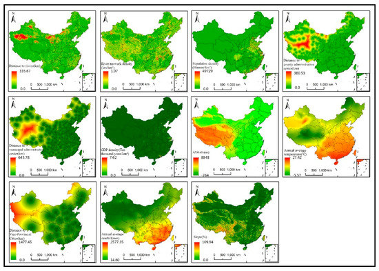
Figure 1.
Driving forces for urban sprawl simulation.
2.1.4. Extraction Methods for Urban Built-Up Areas
Night light data can show the spatial difference and spatial aggregation of human activity intensity. The closer the built-up area to the urban center, the larger its pixel value, while at the edge of the city, the pixel value decreases rapidly. Based on this principle, the Canny edge detection algorithm can effectively detect the boundary information between built-up and non-built-up areas. According to the detected boundary, the segmentation threshold can be calculated to extract the urban built-up areas.
2.2. Data Source
Night light data were obtained from the National Oceanic and Atmospheric (NOAA). We used two types of night light data, i.e., DMSP/OLS and net primary production (NPP/VIIRS). The DMSP/OLS data included the data of a total of 34 night light images from 1992 to 2013, and part of the light data for some years were acquired by different satellites. Night light data were obtained for the years 1992, 1997, 2002, 2007, 2012, and 2017. Although not all data from 1992 to 2013 were required, all 34 images needed to be downloaded for night light data correction. The night light data for 2017 were replaced by NPP/VIIRS data. These data were the monthly composite night light remote sensing data and inherited the basic characteristics of DMSP/OLS stable night light remote sensing data. In the official website of the NOAA, only annual composite products for 2015 and 2016 are provided, and therefore, the data for 2017 needed to be processed using the monthly composite product. Hence, the NPP/VIIRS image data for all 12 months in 2017 were downloaded. DMSP/OLS data are raster data with a spatial resolution of 1000 m × 1000 m. There was no addition data processing for DMSP/OLS. However, NPP/VIIRS data are raster data with a spatial resolution of 500 m × 500 m. Therefore, they were resampled in ArcGIS to a resolution of 1000 m × 1000 m.
The driving factors of urban sprawl can be divided into three categories: environmental factors, socio-economic factors, and distance factors, with a total of 11 indicators (Table 1). Annual average temperature and annual average rainfall data were obtained from the Dataset of China’s Surface Cumulative Annual Value (1981–2010) of the National Meteorological Information Center, which integrated the data of meteorological stations of all provinces, municipalities, autonomous regions, and special administrative regions in China. The original data of temperature and rainfall are vector point data and they are converted into 1000 m × 1000 m raster data through spatial interpolation.

Table 1.
Driving forces of urban sprawl.
Elevation and slope data were derived from the geospatial data cloud. After downloading the national digital elevation model (DEM) data with a resolution of 90 m, the national elevation data were obtained by stitching and resampling those DEM data, and slope data could be generated by processing DEM data with the slope tool in ArcGIS. The elevation and slope data were resampled to a spatial resolution of 1000 m × 1000 m.
River network data, population data, and GDP data were obtained from the Resources and Environment Science Data Center, Chinese Academy of Sciences. Population and GDP data consisted of 1000 × 1000 m spatial grid data. The original data of the river network are vector line data. In ArcGIS, the density and distance tools were used to acquire the spatial raster data of the river network density and the distance to the river network.
The coordinate data of the build-up areas for various kinds of administrative centers were acquired by the Application Program Interface (API) from the Baidu Map. The original data were all vector point data. Since the data of the Baidu Map follow the coordinate system defined by Baidu itself, the obtained data should be processed by coordinate conversion. Subsequently, distance factors could be generated in ArcGIS by using the coordinate data of administrative centers. All the above data were processed into 1000 × 1000 m grid data. The geographical coordinate system was WGS-84, and the projection coordinate system was Albers_Conic_Equal_Area.
3. Results and Analysis
3.1. Simulation Accuracy Test
3.1.1. Probability Accuracy Test of Urban Sprawl Suitability
Whether the urban sprawl suitability results obtained by the above models were reliable needed to be further verified. For the verification of the neural network model, the k-fold cross-validation method was adopted. The k-fold cross-validation has become a common model validation method after a long period of development, and it performs well in terms of model error estimation. The basic principle is to segment the training sample data into k subsets with the same sample number, and then conduct k times of training on the segmented data set. In each training, k−1 sample subsets were used as training datasets, and the remaining sample subset was used as the prediction dataset. The prediction results were obtained by the trained model, and the error of the prediction model was calculated. Finally, after k times of training, k error results were obtained, and their average value was taken as the approximate error value of the model. The advantages of this algorithm are that the sample datasets are randomly segmented and that each data point only appears once in k−1 times of training, which ensures the accuracy of the verification method. Generally, 10-fold cross-validation can meet the test requirements of the model.
Based on the calculation results (Table 2), in the 10-fold cross-validation, all accuracies were greater than 0.8, with a minimum value of 0.810, a maximum value of 0.924, and an average value of 0.864. Overall, the model had a high accuracy and passed the accuracy test. Hence, it can be used to make the suitability map of urban sprawl. By running the model, we can obtain the suitability probability of built-up and non-built-up areas (Figure 2).
Table 2.
Results of k-fold cross-validation.
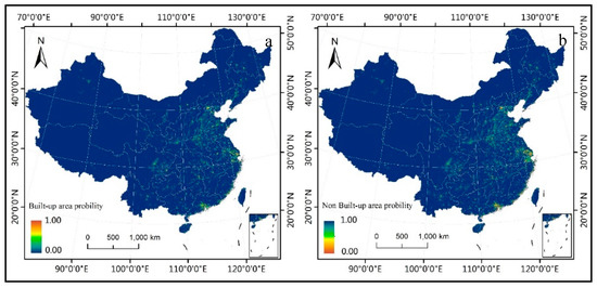
Figure 2.
Suitability probability of built-up and non-built-up areas. Notes: The suitability probability ranges from 0 to 1. A larger value indicates a higher probability of becoming urban areas (a) or non-urban areas (b).
3.1.2. Simulation Accuracy Test of Urban Sprawl
In this study, the full number test method was used to test the simulation results. This method can test each grid data point of the simulation results, leading to a high reliability. In IDRIS, the CROSSTAB tool was used for accuracy verification. This tool crossed the predicted data in 2017 with the extraction results of night light data and was used to obtain the cross-check error graph (Figure 3) as well as the Kappa coefficient of the simulation accuracy test. The Kappa coefficient was 0.78, indicating that the simulation results of urban sprawl by the CA model were of relatively high accuracy. Hence, the ANN-Markov-CA composite model is suitable for the simulation of urban sprawl in China and can guarantee simulation accuracy.
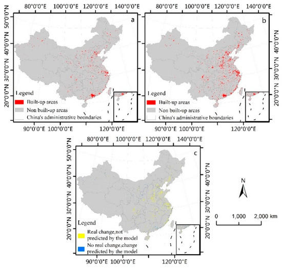
Figure 3.
(a) China’s urban built-up areas in 2017; (b) simulation results of built-up areas in China in 2017; (c) error check.
3.2. Simulation Result Analysis
Taking 2017 as the base year and presetting the prediction interval as five years, we simulated the variation of urban built-up areas in China in 2022, 2027, 2032, and 2037 (Figure 4). We also conducted a comparative analysis on the urban sprawl on two sides of Hu’s line. The term “Hu’s line” represents the boundary line of the spatial distribution of China’s population density, which was discovered by Hu Huanyong. At the same time, Hu’s line is also the dividing line between China’s eastern and western population, economy, and other important human factors. According to the statistics of the simulation results, the urban built-up area in China, the urban built-up area on both sides of Hu’s line, and the proportion of urban built-up areas on both sides of Hu’s line of the total urban built-up area of China from 2022 to 2037 could be obtained (Figure 5).
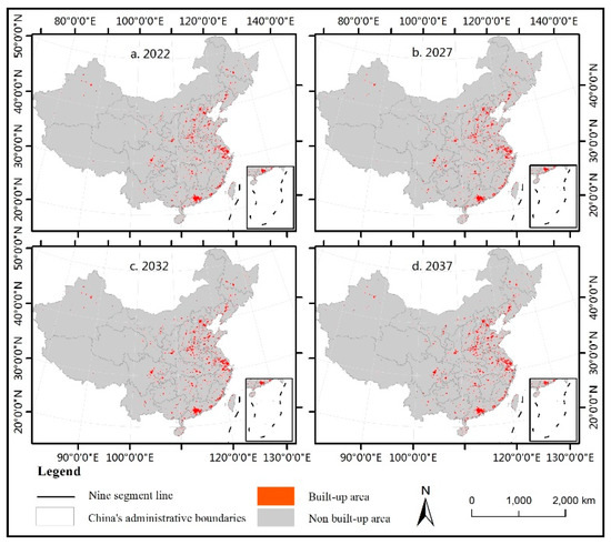
Figure 4.
Simulation results of urban sprawl in China in (a) 2022; (b) 2027; (c) 2032, and (d) 2037.
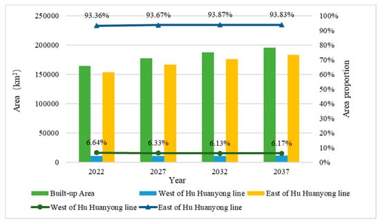
Figure 5.
Predicted built-up areas on the two sides of Hu’s Line from 2022 to 2037.
From 2022 to 2037, the total built-up area in China will gradually increase, along with the urban built-up area on both sides of Hu’s line, while the proportion of urban built-up areas on both sides of Hu’s line will remain unchanged. From 2022 to 2037, on the two sides of Hu’s line, the urban built-up area on the eastern side will account for the highest proportion of the total area in 2022, 2027, 2032, and 2037, with 93.36%, 93.67%, 93.87%, and 93.83%, respectively, which are all above 93%. By contrast, the built-up areas on the western side of Hu’s line will account for about 6% of the total area at each time point. The built-up areas on both sides of Hu’s line will significantly differ. The growth rates of the built-up areas on the eastern side in the three periods of 2022–2027, 2027–2032, and 2032–2037 are predicted to be 8.51%, 5.97%, and 4.08%, respectively, showing a gradual decrease, while those on the western side in the three periods of 2022–2027, 2027–2032, and 2032–2037 are predicted to be 3.21%, 2.44%, and 4.96%, respectively, which are obviously lower than those on the eastern side. Considering the larger base number of the built-up area on the eastern side, the increase in the build-up area on the western side is insufficient to alter the current spatial distribution pattern, according to which urban built-up areas in China are unevenly distributed on the two sides of Hu’s line.
As shown in Figure 6, the urban sprawl from 2022 to 2037 is predicted to be mainly distributed in the central and eastern regions of China; in flat areas such as plains and basins, urban sprawl will be more significant. With Hu’s line as the boundary, the built-up areas will be more distributed and more significantly expanded on the eastern than on the western side. The major areas of urban sprawl in China from 2022 to 2027 will have greatly changed when compared to those from 1992 to 2017. The Pearl River delta and the Yangtze River delta are no longer the major areas of urban sprawl, while the Chengdu-Chongqing city cluster, the Guanzhong Plain city cluster, the Central Plains city cluster, and the middle reaches of the Yangtze River become the new urban sprawl areas. In successive periods from 2027 to 2032 and from 2032 to 2037, the urban sprawl will mainly be distributed around the built-up areas of existing cities, with no significant regions. In spite of this, the area proportion of urban sprawl on both sides of Hu’s line is still considerable. Based on the above analysis, it will be difficult for urban sprawl in China to break the limits of Hu’s line. The Yangtze River delta and the Pearl River delta are no longer the most popular areas for urban sprawl, and the hotspot regions of urban sprawl gradually change from first-tier cities to second- and third-tier cities.
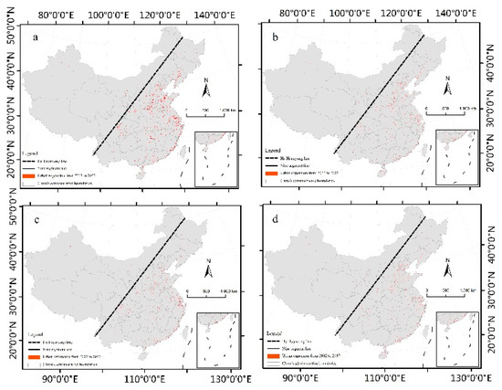
Figure 6.
Spatial distribution of urban sprawl in (a) 2022; (b) 2027; (c) 2032, and (d) 2037.
4. Conclusions
In this study, a total of 11 factors, namely annual average air temperature, annual average precipitation, elevation, slope, river network density, population density, GDP density, distance to rivers, distance to county-level administrative centers, distance to municipal administrative centers, and distance to vice-provincial cities, were selected as driving factors for urban sprawl. The ANN model was developed with Python language, and the suitability of urban sprawl was obtained by training data with those 11 driving force factors. The Markov model was used to predict the increased area of future urban sprawl, combined with the CA model to simulate the urban sprawl of China in 2022, 2027, 2032, and 2037. The simulation results were analyzed, and Hu’s line was introduced to predict urban sprawl on both sides of Hu’s line.
The test accuracy of the suitability evaluation of urban sprawl based on the ANN model was 0.864. This is a relatively high accuracy, indicating that the ANN model is suitable for the suitability evaluation of urban sprawl. The CA-Markov model was used to simulate urban sprawl in China, and the Kappa coefficient was 0.78. This suggests that the CA-Markov model has a high simulation accuracy and is suitable for the simulation of urban sprawl. However, there were also some defects in the simulation. For example, when simulating land use change, it is better to include the protected areas to improve the simulating accuracy and authenticity. Unfortunately, we did not acquire the protected area data of China. Thus, it is possible that the simulated urban sprawl occurs in protected areas which is against the reality. However, since the protected area usually does not distribute to nearby urban areas, this kind of simulation error would not appear a lot. When the CA model is used to simulate land use change, it is necessary to input spatialized driving force data. The spatial resolution of these spatialized driving force data should be the same. Otherwise, the model cannot run. However, because the driving force data involve different types of data, such as natural condition data, economic condition data, and social condition data, it is difficult to obtain all of them from one channel. This also leads to differences in the resolution of different driving force data and the necessity for data format conversion. In the process of data conversion, certain data distortion problems would occur. However, the data processing methods used in this paper were all verified by many previous researches, which can guarantee the accuracy of the data conversion and can retain the valid information of the data to a large degree. At the same time, there may be some distortion problems in the process of data processing. However, considering the huge research area of the paper (the whole mainland China), the impact of a few data distortion problems on the final research results could be small.
In the future, from 2022 to 2037, the hotspot areas of urban sprawl in China will change over time. Although the scale of urban sprawl in the Beijing-Tianjin-Hebei region, the Yangtze River delta, and the Pearl River delta will still be considerable, the urban sprawl scale in the Chengdu-Chongqing city cluster, the Guanzhong Plain city cluster, the Central Plains city cluster, and the middle reaches of the Yangtze River will be more prominent. There will be a large gap between the numbers of urban build-up areas in the eastern and western sides of Hu’s line. Under current environmental and socio-economic conditions, it is difficult for urban sprawl in China to break the limits of Hu’s line in the near future.
The ANN-CA-Markov composite model was used to simulate the future urban sprawl in China. The simulation results demonstrated that the composite model had a higher simulation accuracy and excellent simulation effects. When the CA model was run, the expansion areas were selected according to the suitability probability of urban sprawl, which would result in the aggregation of a large number of new urban built-up areas in a certain region with higher suitability. To solve this problem, the method of regional simulation could be adopted to control the number of newly built areas in a single region, thus further improving the simulation accuracy.
Based on the results of the ANN-Markov-CA composite model, the hotspot areas of urban sprawl will be shifting from first-tier cities to second- and third-tier cities. The limitation of Hu’s line was mainly related to the spatial distribution of China’s natural environment and social and economic conditions. In terms of environmental conditions, the regions east of Hu’s line are subtropical monsoon and temperate monsoon regions, which are affected by water vapor from the Pacific and Indian oceans. They therefore receive sufficient rainfall while also containing numerous flat areas, such as the Northeast Plain, the North China Plain, the Middle and Lower Yangtze River Plain, and the Sichuan Plain, which are conducive to the development of cities. These regions have many large rivers, such as the Yangtze River, the Yellow River, and the Pearl River, as well as lakes such as Poyang Lake, Dongting Lake, and Taihu Lake, with sufficient freshwater resources. In terms of socio-economic conditions, these regions have the three largest city clusters in China: the Beijing-Tianjin-Hebei city cluster, the Yangtze River delta city cluster, and the Pearl River delta city cluster. In addition, they also have a large population base, accounting for 94% of China’s population, and the economic volume far exceeds that of the regions west of Hu’s line, where most areas are plateau, Gobi, and desert areas. Blocked by the Qinghai-Tibet Plateau, these areas receive little precipitation. Most urban areas are distributed in the provincial capitals; there are few cities and the economic volume is small. The level of economic development of these regions differs largely from that of the eastern regions. As a result, the regions east of Hu’s line are comprehensively ahead of the regions west of Hu’s line in terms of population attraction capacity and urban construction and development, which creates a loop in the long-term development and makes it difficult to break Hu’s line.
Author Contributions
Conceptualization, X.Z. and W.S.; methodology, J.Z.; software, J.Z.; formal analysis, X.Z., J.Z. and W.S.; investigation, X.Z.; resources, X.Z. and W.S.; writing—original draft preparation, X.Z. and J.Z.; writing—review and editing, W.S.; supervision, X.Z. and W.S.; funding acquisition, X.Z. and W.S. All authors have read and agreed to the published version of the manuscript.
Funding
This research was funded by the National Natural Science Foundation of China (Grant Nos. 41501202 and 41701100), Research Fund of Hebei University of Economics and Business (Grant No. 2019ZD06) and the Program of the Humanities and Social Sciences Research of Ministry of Education of China (17YJCZH192).
Conflicts of Interest
The authors declare no conflict of interest. The funders had no role in the design of the study; in the collection, analyses, or interpretation of data; in the writing of the manuscript; nor in the decision to publish the results.
References
- Zheng, D.; Zhang, G.; Shan, H.; Tu, Q.; Wu, H.; Li, S. Spatio-Temporal Evolution of Urban Morphology in the Yangtze River Middle Reaches Megalopolis, China. Sustainability 2020, 12, 1738. [Google Scholar] [CrossRef]
- Khanal, N.; Uddin, K.; Matin, M.A.; Tenneson, K. Automatic detection of spationtemporal urban expansion patterns by fusing OSM and Landsat data in Kathmandu. Remote Sens. 2019, 11, 2296. [Google Scholar] [CrossRef]
- Fei, W.; Zhao, S. Urban land expansion in China’s six megacities from 1978 to 2015. Sci. Total Environ. 2019, 664, 60–71. [Google Scholar] [CrossRef]
- Dadashpoor, H.; Salarian, F. Urban sprawl on natural lands: Analyzing and predicting the trend of land use changes and sprawl in Mazandaran city region, Iran. Environ. Dev. Sustain. 2020, 22, 593–614. [Google Scholar] [CrossRef]
- National Bureau of Statistics of China. 2015 China Statistical Yearbook 2015; China Statistical Publishing House: Beijing, China, 2016. [Google Scholar]
- Huang, X.; Schneider, A.; Friedl, M.A. Mapping sub-pixel urban expansion in China using MODIS and DMSP/OLS nighttime lights. Remote Sens. Environ. 2016, 175, 92–108. [Google Scholar] [CrossRef]
- Marais, L.; Denoon-Stevens, S.; Cloete, J. Mining towns and urban sprawl in South Africa. Land Use Policy 2020, 93, 103953. [Google Scholar] [CrossRef]
- Zhou, Y.; Smith, S.J.; Elvidge, C.D.; Zhao, K.; Thomson, A.; Imhoff, M. A cluster-based method to map urban area from DMSP/OLS nightlights. Remote Sens. Environ. 2014, 147, 173–185. [Google Scholar] [CrossRef]
- Elvidge, C.D.; Sutton, P.C.; Tuttle, B.T.; Baugh, K.E.; Howard, A.T.; Erwin, E.H. Change Detection in Satellite Observed Nighttime Lights: 1992–2003. In Proceedings of the 2007 Urban Remote Sensing Joint Event, Paris, France, 11–13 April 2007; pp. 1–4. [Google Scholar]
- Liu, X.; Ning, X.; Wang, H.; Wang, C.; Zhang, H.; Meng, J. A Rapid and Automated Urban Boundary Extraction Method Based on Nighttime Light Data in China. Remote Sens. 2019, 11, 1126. [Google Scholar] [CrossRef]
- Al-Bilbisi, H. Spatial Monitoring of urban expansion using satellite remote sensing images: A case study of Amman City, Jordan. Sustainability 2019, 11, 2260. [Google Scholar] [CrossRef]
- Lo, C.P. Modeling the population of China using DMSP operational linescan system nighttime data. Photogramm. Eng. Remote Sens. 2001, 67, 1037–1047. [Google Scholar]
- Sutton, P.; Roberts, D.; Elvidge, C.; Baugh, K. Census from Heaven: An estimate of the global human population using night-time satellite imagery. Int. J. Remote Sens. 2001, 22, 3061–3076. [Google Scholar] [CrossRef]
- Welch, R. Monitoring urban population and energy utilization patterns from satellite Data. Remote Sens. Environ. 1980, 9, 1–9. [Google Scholar] [CrossRef]
- Raupach, M.R.; Rayner, P.J.; Paget, M. Regional variations in spatial structure of nightlights, population density and fossil-fuel CO2 emissions. Energy Policy 2010, 38, 4756–4764. [Google Scholar] [CrossRef]
- Xu, Z.; Xia, X.; Liu, X.; Qian, Z. Combining DMSP/OLS Nighttime Light with Echo State Network for Prediction of Daily PM2.5 Average Concentrations in Shanghai, China. Atmosphere 2015, 6, 1507–1520. [Google Scholar] [CrossRef]
- Takashima, M.; Hayashi, H.; Kimura, H.; Kohiyama, M. Earthquake damaged area estimation using DMSP/OLS night-time imagery-application for Hanshin-Awaji earthquake. In Proceedings of the IGARSS 2000, IEEE 2000 International Geoscience and Remote Sensing Symposium, Taking the Pulse of the Planet: The Role of Remote Sensing in Managing the Environment (Cat. No.00CH37120), Honolulu, HI, USA, 24–28 July 2000; Volume 331, pp. 336–338. [Google Scholar]
- Trathan, P.N. Remote sensing of the global light-fishing fleet: An analysis of interactions with oceanography, other fisheries and predators. Adv. Mar. Biol. 2001, 39, 261–278. [Google Scholar] [CrossRef]
- Xu, T.; Gao, J. Directional multi-scale analysis and simulation of urban expansion in Auckland, New Zealand using logistic cellular automata. Comput. Environ. Urban Syst. 2019, 78, 101390. [Google Scholar] [CrossRef]
- Gomes, E.; Abrantes, P.; Banos, A.; Rocha, J. Modelling future land use scenarios based on farmers’ intentions and a cellular automata approach. Land Use Policy 2019, 85, 142–154. [Google Scholar] [CrossRef]
- Huang, Q.; Song, W. A land-use spatial optimum allocation model coupling a multi-agent system with the shuffled frog leaping algorithm. Comput. Environ. Urban Syst. 2019, 77, 101360. [Google Scholar] [CrossRef]
- Geng, B.; Zheng, X.; Fu, M. Scenario analysis of sustainable intensive land use based on SD model. Sustain. Cities Soc. 2017, 29, 193–202. [Google Scholar] [CrossRef]
- Chotchaiwong, P.; Wijitkosum, S. Predicting urban expansion and urban land use changes in Nakhon Ratchasima City using a CA-Markov Model under two different scenarios. Land 2019, 8, 140. [Google Scholar] [CrossRef]
- Zhao, Z.; Guan, D.; Du, C. Urban growth boundaries delineation coupling ecological constraints with a growth-driven model for the main urban area of Chongqing, China. GeoJournal 2019, 4, 1–17. [Google Scholar] [CrossRef]
- Quan, Q.; Tian, G.; Sha, M. Dynamic simulation of Shanghai urban expansion based on multi-agent system and cellular automata models. Shengtai Xuebao/Acta Ecol. Sin. 2011, 31, 2875–2887. [Google Scholar]
- Gounaridis, D.; Chorianopoulos, I.; Symeonakis, E.; Koukoulas, S. A Random Forest-Cellular Automata modelling approach to explore future land use/cover change in Attica (Greece), under different socio-economic realities and scales. Sci. Total Environ. 2019, 646, 320–335. [Google Scholar] [CrossRef] [PubMed]
- Ye, Y.; Su, Y.; Zhang, H.-o.; Liu, K.; Wu, Q. Construction of an ecological resistance surface model and its application in urban expansion simulations. J. Geogr. Sci. 2015, 25, 211–224. [Google Scholar] [CrossRef]
- Firozjaei, M.K.; Sedighi, A.; Argany, M.; Jelokhani-Niaraki, M.; Arsanjani, J.J. A geographical direction-based approach for capturing the local variation of urban expansion in the application of CA-Markov model. Cities 2019, 93, 120–135. [Google Scholar] [CrossRef]
- Cilliers, S.S.; Bredenkamp, G.J. Vegetation of road verges on an urbanisation gradient in Potchefstroom, South Africa. Landsc. Urban Plan. 2000, 46, 217–239. [Google Scholar] [CrossRef]
- Fu, X.; Wang, X.; Yang, Y.J. Deriving suitability factors for CA-Markov land use simulation model based on local historical data. J. Environ. Manag. 2018, 206, 10–19. [Google Scholar] [CrossRef]
- Zhao, M.; He, Z.; Du, J.; Chen, L.; Lin, P.; Fang, S. Assessing the effects of ecological engineering on carbon storage by linking the CA-Markov and InVEST models. Ecol. Indic. 2019, 98, 29–38. [Google Scholar] [CrossRef]
- Aburas, M.M.; Ho, Y.M.; Ramli, M.F.; Ash’aari, Z.H. Improving the capability of an integrated CA-Markov model to simulate spatio-temporal urban growth trends using an Analytical Hierarchy Process and Frequency Ratio. Int. J. Appl. Earth Obs. Geoinf. 2017, 59, 65–78. [Google Scholar] [CrossRef]
- Varga, O.G.; Pontius, R.G.; Singh, S.K.; Szabó, S. Intensity Analysis and the Figure of Merit’s components for assessment of a Cellular Automata—Markov simulation model. Ecol. Indic. 2019, 101, 933–942. [Google Scholar] [CrossRef]
- Siddiqui, A.; Siddiqui, A.; Maithani, S.; Jha, A.K.; Kumar, P.; Srivastav, S.K. Urban growth dynamics of an Indian metropolitan using CA Markov and Logistic Regression. Egypt. J. Remote Sens. Space Sci. 2018, 21, 229–236. [Google Scholar] [CrossRef]
- Gidey, E.; Dikinya, O.; Sebego, R.; Segosebe, E.; Zenebe, A. Cellular automata and Markov Chain (CA_Markov) model-based predictions of future land use and land cover scenarios (2015–2033) in Raya, northern Ethiopia. Modeling Earth Syst. Environ. 2017, 3, 1245–1262. [Google Scholar] [CrossRef]
- Li, X.; Yeh, A.G.-O. Calibration of Cellular Automata by Using Neural Networks for the Simulation of Complex Urban Systems. Environ. Plan. A Econ. Space 2001, 33, 1445–1462. [Google Scholar] [CrossRef]
- Yeh, A.G.-O.; Li, X. Simulation of development alternatives using neural networks, cellular automata, and GIS for urban planning. Photogramm. Eng. Remote Sens. 2003, 69, 1043–1052. [Google Scholar] [CrossRef]
- Song, W.; Deng, X.Z. Land-use/ land-cover change and ecosystem service provision in China. Sci. Total Environ. 2017, 576, 705–719. [Google Scholar] [CrossRef] [PubMed]
- Rimal, B.; Keshtkar, H.; Sharma, R.; Stork, N.; Rijal, S.; Kunwar, R. Simulating urban expansion in a rapidly changing landscape in eastern Tarai, Nepal. Environ. Monit. Assess. 2019, 191, 255. [Google Scholar] [CrossRef]
- Zhang, Y.; Li, X.; Song, W. Determinants of cropland abandonment at the parcel, household and village levels in mountain areas of China: A multi-level analysis. Land Use Policy 2014, 41, 186–192. [Google Scholar] [CrossRef]
- Zubair, O.A.; Ji, W.; Festus, O. Urban expansion and the loss of Prairie and agricultural lands: A satellite remote-sensing-based analysis at a Sub-watershed scale. Sustainability 2019, 11, 4673. [Google Scholar] [CrossRef]
- Song, W.; Pijanowski, B.C. The effects of China’s cultivated land balance program on potential land productivity at a national scale. Appl. Geogr. 2014, 46, 158–170. [Google Scholar] [CrossRef]


© 2020 by the authors. Licensee MDPI, Basel, Switzerland. This article is an open access article distributed under the terms and conditions of the Creative Commons Attribution (CC BY) license (http://creativecommons.org/licenses/by/4.0/).