A Novel Smart Energy Management as a Service over a Cloud Computing Platform for Nanogrid Appliances

Abstract

There will be a dearth of electrical energy in the world in the future due to exponential increase in electrical energy demand of rapidly growing world population. With the development of Internet of Things (IoT), more smart appliances will be integrated into homes in smart cities that actively participate in the electricity market by demand response programs to efficiently manage energy in order to meet this increasing energy demand. Thus, with this incitement, the energy management strategy using a price-based demand response program is developed for IoT-enabled residential buildings. We propose a new EMS for smart homes for IoT-enabled residential building smart devices by scheduling to minimize cost of electricity, alleviate peak-to-average ratio, correct power factor, automatic protective appliances, and maximize user comfort. In this method, every home appliance is interfaced with an IoT entity (a data acquisition module) with a specific IP address, which results in a wide wireless system of devices. There are two components of the proposed system: software and hardware. The hardware is composed of a base station unit (BSU) and many terminal units (TUs). The software comprises Wi-Fi network programming as well as system protocol. In this study, a message queue telemetry transportation (MQTT) broker was installed on the boards of BSU and TU. In this paper, we present a low-cost platform for the monitoring and helping decision making about different areas in a neighboring community for efficient management and maintenance, using information and communication technologies. The findings of the experiments demonstrated the feasibility and viability of the proposed method for energy management in various modes. The proposed method increases effective energy utilization, which in turn increases the sustainability of IoT-enabled homes in smart cities. The proposed strategy automatically responds to power factor correction, to protective home appliances, and to price-based demand response programs to combat the major problem of the demand response programs, which is the limitation of consumer’s knowledge to respond upon receiving demand response signals. The schedule controller proposed in this paper achieved an energy saving of 6.347 kWh real power per day, this paper achieved saving 7.282 kWh apparent power per day, and the proposed algorithm in our paper saved $2.3228388 per day.

1. Introduction

Internet of Things (IoT) is a paradigm that bridges a variety of real, digital, and virtual devices through information networks into smart environments and spans across domains such as energy, transportation, cities, etc. [1]. An important and rapidly growing application of the IoT is the smart grid/nanogrid. The smart grid/nanogrid is an important domain of the Internet of Things (IoT), which aims to achieve reliable information transmission through smart facilities (e.g., smart meters) and realize real-time control, accurate management, and scientific decision-making of the smart grid/nanogrid by smart devices [2]. The smart grid seeks to increase performance, dependability, and protection via automation and advanced technologies of communication [3,4].

In the nanogrid, the capacity to make self-decisions is one of the most essential features that businesses create and deliver to customers. To enable the self-decision-making ability in a nanogrid, utilities developed effective and viable demand response (DR) mechanisms for electrical energy management/demand side management (DSM).

In a nanogrid, DSM refers to programs and innovations that enable the end customers to optimize their energy of electrical consumption, while enhancing the stability and efficiency of the compromises in the conventional nanogrid grid. The first important move to participate in DR programs/DSM at a nanogrid is to monitor fine grain electrical energy in the realistic areas of interest consumed by each major electrical unit. For example, a smart home energy management system (EMS), which is connected to the nanogrid via advanced metering infrastructure (AMI), can be used in DSM/e-energy management, using smart plug-ins which connect to an AMI power supply smart meter and keep track of energy consumption for each major app [5].

The home energy management system (HEMS) is a core feature of the smart grid. The HEMS aims at lowering energy cost to customers and enhancing comfort levels of customers while ensuring grid reliability [6]. In addition, the physical quantities determined by (HEMS) exhibit broader range, greater frequency, and improved grain size than earlier when backed by the advanced metering infrastructure (AMI) technology [7].

Worldwide adoption of HEMSs, which recognize and communicate electricity consumption data through invasive smart plug deployments, leads to modern, user-focused, DSM-based IoT applications. It is based on a central cloud architecture model that generates large quantities of data that must be distributed, saved, and processed in powerful cloud computing in smart homes in the nanogrid. IoT devices are deployed. Cloud-centered analytics of data science, cloud analytics, is focused on the non-restrictive or not always accessible network connectivity/internet, typically inappropriate for the nanogrid’s user-centric latency-oriented IoT applications for smart home services [8]. In comparison with cloud analysis, where data collected and transmitted through IoT terminals to the cloud are handled via centralized cloud-centric analysis, fog analysis is an advanced technique devoted to and used for the analysis of the data that must be processed immediately for analytical, interpretable, and accurate data in IoT sources. Compared with cloud analysis, fog analysis is extended. This means that for latency-sensitive user-focused IoT application in intelligent homes, artificial intelligent models are trained in cloud analysis and then deployed on-site on IoT ends, as edge analysis at the edge of internet and edge analytics, which immediately support analytical, interpretable, and real-time operative data insights at IoT sources are required.

In applications of energy management, wireless sensor networks (WSNs) play a major part, rendering smart grids open to homes. Wireless connectivity also has certain benefits over wired communication, such as low-cost setups and quick access to remote or inaccessible places. Today there are many smart home wireless communication technologies: Infrared, Home RF, ZigBee, Z-wave, Wi-Fi, Bluetooth, etc. [9].

The effective usage of electricity in smart homes saves resources, boosts efficiency, and ultimately lowers carbon footprint. Therefore, for smart homes and intelligent cities, the necessity of smart management of energy is growing. Nonetheless, the absence of low cost, simple to use and low-maintenance technologies has reduced a widespread implementation of such setups to some degree [10].

In particular, daily and seasonal changes in energy output and demand profiles, significant energy storage costs, and the responsive balance between grid stability and flexibility are among the most troublesome aspects, due to a large number of technical and economic problems associated with the high rate of penetration into the electrical grid [11].

To deal with such issues, suitable energy management systems have been discussed in the technical literature [12,13,14]. Monitoring and optimizing of power flow are the main functions of EMSs. These systems allow consumers to be actively engaged on the energy market at the end-user level. On the other hand, they provide support to a grid operator in terms of optimized decisions, for example implementing demand side management schemes [15,16].

Energy management systems are also useful for the industrial and commercial sectors when it comes to intelligent homes where various types of device elements (e.g., software algorithms, hardware elements, network links, and sensors) collaborate together to provide different services supporting the human lifestyle [11]. A framework for energy management should display unique features that are useful to the end-user. Besides providing a commodity and an advantage, it should easily fit into a home appliance setup, it should require a smooth set-up and a minimal amount of cabling, and it should not be bulky. Therefore, it is also important to examine how to incorporate and integrate them more effectively into an intelligent household, apart from research into the practical aspects of energy management systems (e.g., how they are described, configured, and which technique they use) for their real-world implementation. The IoT paradigm is currently the preferred approach to this goal.

For latency sensitive user centric IoT applications in DSM, edge analytics are required to ensure the immediate analysis, interpretation, and real-time operating information processed and detected by an IoT system in the IoT sources and are collaborated with the cloud analytics. Additionally, much attention remains to be paid in conducting and applying fog-cloud analytics in smart homes, as examples, for demand-side management in a nanogrid. Therefore this work develops and implements a prototype of intelligent analytical power meters, intelligent algorithms for smart home demand side management.

2. Knowledge and Objectives

In ref. [17], hybrid meta-heuristic techniques for scheduling of appliances are proposed. The main point of designing a hybrid technique is a balance of exploration and exploitation. In order to achieve this balanced hybrid of optimal stopping rule (OSR) with genetic algorithm (GA), teaching learning based optimization (TLBO) and the Firey algorithm (FA) are proposed. The objective of this research is to reduce energy consumption and minimize waiting time along with peak-to-average ratio and cost as optimized parameters. MATLAB simulation has been conducted while considering user priorities, and RTP for heterogeneous homes. The limitation of the proposed methodology is the use of a limited number of appliances. This proposed scheme has not considered the effect of HVAC, which is the major energy consumer in the residential sector.

A hybrid technique uses two optimization approaches of bacterial foraging algorithm (BFA) and GA [18] with the objective of reducing cost and peak to average ratio (PAR). PAR is one of the important performance metrics used to evaluate how peak electricity consumption affects the system. There are a variety of appliances that require either high voltage or low voltage. DSM persuades the electricity consumer to shift the high voltage required appliances to the low peak hours so that less energy is consumed during peak hours. However, most of the schedulers often result in the increase of PAR, as they increase the load during low peak hours. The proposed algorithm used the fitness function of cost reduction, but it also minimizes peak to average ratio (PAR) using day ahead real time price (RTP).

A novel air conditioning system [19] was developed for better demand response by shifting the load in order to balance the power of the smart grid. The proposed system used two demand response strategies named the demand-side bidding (DSB) strategy and demand as frequency-controlled reserve (DFR) strategy. The objective of the study was cost and energy saving while considering a building in Hong Kong with the synthetic dynamic price for RTP. The proposed system only works for the office building. Simulations are performed for the 40-story building using EnergyPlus by comparing the conventional air conditioning approach and proposing an approach that a results in reduction in cost and energy use.

In ref. [20] paper, a fuzzy logic rule-based algorithm is developed along with wireless sensors integration. A wireless programmable thermostat is simulated in MATLAB GUI. The proposed system uses outdoor temperature, load demand, electricity price, and user occupancy parameters in real-time to reduce the thermostat set points for better energy utilization in heating/cooling systems. Performance metrics are demand response participation, energy consumption, and occupants user comfort. The center of gravity (COG) method is used for defuzzication, whereas membership functions of parameters are defined as a triangular shape. As the output parameter decides how much load reduction should be done, the defuzzied value reveals by how much value an initialized set point will change. The objective of the research is to reduce energy consumption while having the best indoor temperature, but user comfort is sacrificed.

In ref. [21], an energy consumption management approach considers household users, in which each house consists of two types of requests or demands: (i) essential and (ii) flexible, where flexible demands are further delay-sensitive and delay-tolerant. To optimize energy for both delay-sensitive and delay-tolerant demands, a new centralized algorithm is presented for scheduling. This approach also aims to reduce the aggregated electricity bill and delay of the flexible demands for achieving the optimum power decisions. The authors design a cost-efficient demand-side day-ahead bidding process and RTP mechanisms by using fractional programming methods in [22].

Article [23] formulated the finite time horizon by considering the 30 min time-slot and modeled mixed-integer non-linear programming using RTP tariff for scheduling. The proposed scheme schedules the electrical and thermal appliances of a smart home. This scheme reduces 22.2% cost for peak price and 11.7% for normal price scheme while shifting the peak load on the thermal resources. Authors in [24] proposed linear programming based optimal scheduling technique to minimize the electricity cost while focusing on energy storage. The discussed technique saved 20.39% average cost and reduced 21.6% average peak load.

In ref. [25] authors proposed a dynamic choice artificial neural network (DCANN). This model is used for day-ahead price forecasting. This model is a combination of supervised and unsupervised learning, which deactivates the bad samples and search optimal inputs for a model to learn. In ref. [26], authors proposed an energy efficient delivery system (ECDS) to analyze the performance of D2D delivery. D2D is robust and efficient. It does not need any knowledge of content distribution, device mobility, and user demand. ECDS is used to minimize the energy consumption of smart cities. This system achieves the optimal solution for a random and dynamic environment. ECDS only performed a few logical operations by utilizing local information of each device to make decisions. After getting information through the green communication system about the usage of different devices, The smart grid can easily forecast the load of power consumption of consumers. In ref. [27], the authors described the local energy market (LEM) concept with an operational auction mechanism. Private blockchain is used for a small size community that determined the prices, based on agents’ order in a decentralized way. Agents participate in a market for short term electricity trading. Photo voltaic (PV) panels are used to produce electricity. A market is designed for a small community in which consumers and prosumers are acting as agents. The authors also forecast the prices of electricity according to the consumption and generation of electricity.

In ref. [28], the author has applied the differential development algorithm which limits the cost of home appliances to users and electricity. On the other hand, the impact of more bill payments on low energy use impacted lower power usage users. In ref. [29], the researchers proposed a home-energy management system, which offers usage particulars of individual product use and enables customers to decide. There is, however, no method for automating the function of the appliance. In ref. [30] the author used harmony search-echo state networks algorithms, particle swarm optimization, and recursive least squares to tune ESN for better prediction. Similar work is reported in [31], where the grey wolf optimization algorithm is used to tune fuzzy control system parameters in order to reduce computational cost.

The researchers in [10] measured the performance of the EMS by taking into account data on power use, room temperature, ambient temperature, and customer use profile before and post EMS setup implementation. Considerable power decreases are said to be accomplished by adjusting the TV use pattern, eliminating standby power usage and modifying the refrigerator capabilities on the basis of the above stated restrictions. In ref. [32], the researchers used algorithms for optimized real-time scheduling devised to adjust the peak window and reduce general energy usage by prioritizing devices. In ref. [33], the authors concentrated on more complex circumstances, where power and electricity costs for electrical appliances operations with the overall grid charge are not shiftable, and renewable energy production is uncertain. The artificial neural network was used in [34] to change the weights for the agglomeration in order to adjust the prediction intervals using the genetic algorithm and the simulated ringing algorithms. This will reduce the uncertainties and disruptions with the prediction. The researchers in [35] implemented a protocol to maximize the WSN by means of a design for a smart home. This design consists of two settings, external and internal, interacting by means of an access point. The home of the consumer can be managed with a smartphone any time and from anywhere. For the deployment and deferent validation checks, the SQLite database framework was utilized. An IoT technology for smart housing monitoring and surveillance has been introduced in [36]. In other terms, it enables users to access and manage devices by means of touch or voice commands, including the protection net. App Inventor and Android Studio have created this program. In ref. [37] for IoT devices in the intelligent grid, a fog-based architecture is created. The goal of this work is to provide the IoT smart grid with latency-sensitive monitoring, localization awareness, and smart control. In order to extend computing to the edge of the network, a novel fog based architecture is further developed. The experimental analysis reveals the efficiency over other equivalents of their proposed model.

Chilipirea et al. [38] suggested a way of developing IoT models which promote, in a home safety mechanism, the creation of strong energy-efficient setups. The model overlapped the features of the devise to conserve and momentarily deactivate some of the energy. In ref. [39], the authors used an algorithm of optimization on embedded devices but did not explain the algorithm specifics. Additionally, only rule-based EMSs or short-term controllers were introduced. For example, some works implemented very simple on/off device switching functionalities based either on the hour of the day and the presence of users [40] or on a user-selected power consumption limit [41]. In ref. [42], a shedding algorithm and a design of an intelligent home energy management system is suggested. The work was focused on grid management, domestic sources of renewable energy, wireless connectivity between household appliances, a control mechanism, and a home management mechanism. In ref. [43], the authors present an EMS platform of buildings that are based on a distributed agent. The cloud-based architecture that permits data collection, control of devices, and the definition of energy management systems as cloud-based services is presented in [44].

The researchers in [45] demonstrated a smart mechanism for energy-efficient IoT-based households having a cooling system. The heat dissemination in the kitchen region and virtual model of flow was exhibited. When a person exits or reaches the kitchen, the mechanism remotely regulates heating/cooling and illumination.

In ref. [46], the authors showed that they considered fog cloud computing as the Open Fog reference architectural smart home system. The simulation system has not, however, been tested in a realistic environment; the analysis lacked a functional evaluation. Furthermore, the study lacked proof of the analytical capabilities with which AI is trained in cloud analytics and deployed on-site in IoT end devices as edge analytical systems for user-centered IoT applications in intelligent homes. The authors in [47] sought to build a multi-layer cloud architectural model that enables efficient operations/interactions on heterogeneous IoT appliances from various IoT smart houses. In order to support the protection and privacy conservation during the interaction/operation of heterogeneous IoT devices, an ontology-based security service architecture was developed and utilized. In ref. [48], the authors propose a home administration self-learning system that consists of (1) an EMS, (2) a DSM system, and (3). For real-time operation of a smart house, the three parts of the house management system were created and incorporated. The unified, integrated domestic management system involves price forecasts, price clusters, and the power alerting system capabilities for the management of intelligent domestic electricity.

The EMS depends on MQTT, is driven by business intelligence (BI) and analytics, and utilizes big data. The method has been tested using HVAC for the simulation of small residential region structures. A control technique for digital power factor correction (PFC), centered on the speed of the digital signal processor, has been proposed in [49] to address the issue of restricted frequency of switching. A microcontroller was utilized in [50] for regulating switch capacitors for PFC near single-phase electric appliances. Depending on the load, the power factor has various limitations. A new methodology for learning-based optimization (TLBO) was explored, more intricate PFC decision algorithm was scrutinized and a cloud-driven data warehouse for electronic parameters was examined in [51].

In brief, the introduction of the platform for energy management raises the significant challenges stated below:

(1)

Output, interactivity, and interoperability in heterogeneous appliances within an energy management platform.

(2)

Capacity to tailor the adaptability, services, and scalability of the energy management program to different kinds of houses, buildings, and devices.

(3)

Costs of the energy management framework, hardware, and software stack deployment.

To address the above-mentioned challenges, a novel platform for energy management system is proposed that employs interoperability, adaptability, scalability, and connectivity between smart appliances over the cloud computing platform.

The key contributions are summed up here:

• We formulate the energy management and sharing economy problem and present the optimal approach to tackle this problem based on cloud computing.
• We propose a cost and imported electricity minimization scheme to make the environment greener.
• Another contribution of this paper is the proposal of a MAS for micro-grid representation that integrates IoT devices for energy management inside the buildings. The proposed MAS was developed for low-performance hardware, such as single-board computers. This helps agents to be installed in inexpensive and sufficiently compact hardware in the building’s electrical switchboard. The proposed MAS, however, utilizes strong IoT device penetration to conduct energy management solutions within buildings. This is the most critical addition by this work.
• A communication protocol based on IoT and proven specifications such as MQTT, which allows the system to be flexible, is proposed in this study. Furthermore, analytics and business intelligence (BI) are provided in the proposed system, offering a profound insight on the data gathered by visualizing dashboards and reporting. In addition, the usage of data storage technologies based on Big Data enables system scalability at the national level, offering energy efficiency systems for both household owners and utilities companies.
• The appliances presented in this paper capitalize on the developments in information and communication technology (ICT) to build a new telemetry methodology and remote power factor correction. This method is versatile and flexible so as to respond to multiple loads, adjusting the capacitance stages and power factor correction unit settings effectively.
• A hierarchical two-layered communication architecture, which is founded on MQTT protocol and utilizes a cloud based server named Node Red, is implemented to realize local and global communications required for neighborhood appliance controllers.
• A cloud-based platform is developed to store data and share energy among smart users.

3. Methodology

This section describes the modelling methodology for proposed energy management system. Energy management is a key objective in this paper to minimize the electricity cost and automate the protection of devices by appliance scheduling and correct power factor. The proposed framework using Wi-Fi technology for the smart community energy systems is illustrated in Figure 1.

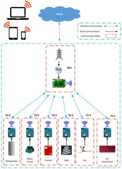
Figure 1. Structure of proposed nanogrid.

The home energy management is a service platform for consumers to monitor and control demand side management effectively. It comprises house devices linked by an integrated device network with consumer comfort as preference. The framework can be used for the control of energy use by various forms of community houses.

At its heart, IoT is an extensive-ranging system of everyday detailed objects connected to the internet, capable of identifying themselves and informing data to objects on an internet network. In our study, IoT is used as a web server for WiFi clients, which are represented by terminal units (TUs), using the BSU (Raspberry Pi3), and all appliances and sensors are connected to these TUs. All home parameters could be related to the Internet to develop IoT structures via this topology. The proposed framework of Raspberry Pi3 and WeMos-D1 was constructed for the MQTT (message queue telemetry transportation) broker. As the portal for the IoT services, the MQTT broker monitored and managed the smart home devices. The advantage of the Internet portal is that the home devices are handled from anywhere in the world. Figure 1 displays the proposed nanogrid system.

3.1. Smart Device Classification

The tasks of consumer usability have been achieved, as future consumers of intelligent devices have been diverse in houses such as launders, boilers, dish washers, fridges, TVs, heating, and lighting systems. There are two key types of devices below: The shiftable devices are controlled and scheduled over scheduling periods times by the energy management system ($\mathcal{T}=24$). These machines are scheduled to reduce the energy bill from one slot to other time slot. Shiftable equipment has a particular load profile in which versatile delays occur in the stable period of consumption. For example, the washing machine, vacuum cleaner, dishwasher, and dryer, and so on. Suppose the handling system collection is denoted as ${\mathcal{D}}_{𝓂,𝓃}$ and ${𝒹}_{𝓂}=1,\dots ,{\mathcal{D}}_{𝓂,𝓃}$ for $𝓃\in \mathcal{N}$ for each user [52].

$${ℒ}_{𝓂,𝓃}={\displaystyle \sum }_{{𝒹}_{𝓂}\in {\mathcal{D}}_{𝓂}}{ℒ}_{{\mathcal{D}}_{𝓂,𝓃}}$$

(1)

where ${ℒ}_{𝓂,𝓃}$ is manageable devices load profile and ${\mathcal{D}}_{𝓂,𝓃}$ is the manageable devices set.

During operating times $\in \mathcal{T}$, the energy usage of non-shiftable devices is constant. Unchanging equipment cannot be moved to full time for scheduling and cost savings. Electrical energy consumer profiles include lamps, ventilators, refrigerators, television, etc. Let us define a group of user nonshiftable devices as:

$${\mathit{ℒ}}_{\mathit{𝓷}\mathit{𝓶},\mathit{𝓷}}={\displaystyle \sum }_{{\mathit{𝓭}}_{\mathit{𝓷}\mathit{𝓶}}\in {\mathcal{D}}_{\mathit{𝓷}\mathit{𝓶}}}{\mathit{ℒ}}_{{\mathcal{D}}_{\mathit{𝓷}\mathit{𝓶},\mathit{𝓷}}}$$

(2)

The aspiration of an optimization model is to schedule a limited resource of energy for operation of devices based on their period preference and cost of electricity. The devices are operating based on 24 h ahead Time of Uses (ToU) electricity tariff. Here, ${ℒ}^{𝓃,𝓉}$ is total power consumption of users $𝓃\in \mathcal{N}$ in $𝓉\in \mathcal{T}$ time slot.

The optimization model aims at estimating the limited energy resource for the service of equipment on the basis of their choice for time and electricity costs. Electrical equipment works under the tariff on energy 24 h ahead of time (TOU). Here, ${ℒ}^{𝓃,𝓉}$ is the total individual power consumption profile of user $𝓃\in \mathcal{N}$ in $𝓉\in \mathcal{T}$ time slot.

$${\mathit{ℒ}}_{\mathit{𝓭}}^{\mathit{𝓷}}={\mathit{ℒ}}_{\mathit{𝓶},\mathit{𝓷}}+{\mathit{ℒ}}_{\mathit{𝓷}\mathit{𝓶},\mathit{𝓷}}$$

(3)

$${\mathit{ℒ}}_{\mathit{𝓭}}^{\mathit{𝓷},\mathit{𝓽}}={\displaystyle \sum }_{\mathit{𝓽}=\mathbf{1}}^{\mathcal{T}}{\mathit{ℒ}}_{\mathit{𝓭}}^{\mathit{𝓷},\mathit{𝓽}}$$

(4)

In community of $\mathcal{N}$ user, ${ℒ}_{\mathcal{T}}$ is the total combined power profile of all customers in community. Let denote ${ℒ}^{𝓃,𝓉}$ be a power profile of user $𝓃\in \mathcal{N}$ at time $𝓉\in \mathcal{T}$,

$${\mathit{ℒ}}_{\mathcal{T}}={\displaystyle \sum }_{\mathit{𝓷}\mathbf{\in }\mathcal{N}}{\displaystyle \sum }_{\mathit{𝓽}\mathbf{\in }\mathcal{T}}{\displaystyle \sum }_{\mathit{𝓭}\mathbf{\in }\mathcal{D}}{\mathit{ℒ}}_{\mathit{𝓭}}^{\mathit{𝓷},\mathit{𝓽}}\mathbf{\forall }\mathit{𝓽}\mathbf{\in }\mathcal{T}$$

(5)

In order to minimize the facts and different demand peaks in other periods of the day, each customer has their own energy consumption schedule. For evaluating the peak to average (PAR) ratio [52], a combined power profile is used. This is the characteristic shape of all machine demand. In Equations (6)–(8), PAR is defined. Calculate the peak and average load levels in this regard first.

$${\mathit{ℒ}}_{\mathit{p}\mathit{e}\mathit{a}\mathit{k}}=\mathit{m}\mathit{a}\mathit{x}{\mathit{ℒ}}_{\mathcal{T}}$$

(6)

$${\mathit{ℒ}}_{\mathit{a}\mathit{v}\mathit{g}}=\frac{\mathbf{1}}{\mathcal{T}}{{\displaystyle \sum }}_{\mathit{𝓷}=\mathbf{1}}^{\mathcal{N}}{{\displaystyle \sum }}_{\mathit{𝓽}=\mathbf{1}}^{\mathcal{T}}{\mathit{ℒ}}^{\mathit{𝓷},\mathit{𝓽}}\mathbf{\forall }\mathit{𝓽}\mathbf{\in }\mathcal{T}$$

(7)

$$\mathit{P}\mathit{A}\mathit{R}=\frac{{\mathit{ℒ}}_{\mathit{p}\mathit{e}\mathit{a}\mathit{k}}}{{\mathit{ℒ}}_{\mathit{a}\mathit{v}\mathit{g}}}$$

(8)

3.2. Formulation of Problem

The objective function minimizes the running costs for the devices in individual and community users. The community users have preferences with regard to their idle modes of operating. Equation (9) objective function and constraints in equations below [52].

$$\begin{gathered} \mathit{m}\mathit{i}\mathit{n}{\mathfrak{P}}_{\mathit{𝓷}}={\displaystyle \sum }_{\mathit{𝓷}\mathbf{\in }\mathcal{N}}{\displaystyle \sum }_{\mathit{𝓽}\mathbf{\in }\mathcal{T}}{\displaystyle \sum }_{\mathit{𝓺}\mathbf{\in }\mathcal{Q}}{\displaystyle \sum }_{\mathit{𝓭}\mathbf{\in }\mathcal{D}}({\mathit{\alpha }}_{\mathit{𝓺}\mathit{𝓭}}^{\mathit{𝓷},\mathit{𝓽}}\times {\mathit{ℒ}}_{\mathit{𝓺}\mathit{𝓭}}^{\mathit{𝓷},\mathit{𝓽}}\times {\mathfrak{P}}_{\mathit{ℰ}}^{\mathit{𝓷},\mathit{𝓽}}-{\mathit{\beta }}_{\mathit{𝓻}}^{\mathit{𝓷},\mathit{𝓽}}\times {\mathfrak{S}}_{\mathit{𝓻}}^{\mathit{𝓷},\mathit{𝓽}}\times {\mathfrak{P}}_{\mathit{𝓻}}^{\mathit{𝓷},\mathit{𝓽}} \\ \hspace{1em}\hspace{1em}\hspace{1em}\hspace{1em}\hspace{1em}\hspace{1em}+{\mathit{\gamma }}_{\mathfrak{P}}^{\mathit{𝓷},\mathit{𝓽}}\times {\mathfrak{L}}_{\mathfrak{L}}^{\mathit{𝓷},\mathit{𝓽}}\times {\mathfrak{P}}_{\mathfrak{P}}^{\mathit{𝓷},\mathit{𝓽}}) \end{gathered}$$

(9)

where, ${\gamma }_{\mathfrak{P}}^{𝓃,𝓉}$ is the decision variable for energy storage, $\mathcal{N}$ is the total users number, $\mathcal{T}$ is a time, $\mathcal{Q}$ is load type, $\mathcal{D}$ is the total devices number, ${\alpha }_{𝓆𝒹}^{𝓃,𝓉}$ is the decision variable for devices scheduling, ${\mathfrak{P}}_{ℰ}^{𝓃,𝓉}$ is electricity cost with respect to time $𝓉$, ${\mathfrak{S}}_{𝓻}^{𝓃,𝓉}$ is the decision variable for energy, ${\mathfrak{L}}_{\mathfrak{L}}^{𝓃,𝓉}$ is electricity storage at time $𝓉$, and ${ℒ}_{𝓆𝒹}^{𝓃,𝓉}$ is the power profile of home load devices with respect to time $𝓉$,

3.2.1. Period Preference of Operation

The willing factor of devices operation, the binary matrix, is used. This provides the time to run the devices in a t time slot with the desired ${𝓌}_{𝓆𝒹}^{𝓃,𝓉}$. Therefore, home users tend to run some equipment more during one day and substitute it with other equipment. These devices work according to the preference for the operating period.

$${\mathfrak{P}}_{\mathbf{1}}:{\mathit{\alpha }}_{\mathit{𝓺}\mathit{𝓭}}^{\mathit{𝓷},\mathit{𝓽}}={\mathit{\alpha }}_{\mathit{𝓺}\mathit{𝓭}}^{\mathit{𝓷},\mathit{𝓽}}\times {\mathit{𝔀}}_{\mathit{𝓺}\mathit{𝓭}}^{\mathit{𝓷},\mathit{𝓽}}$$

(10)

3.2.2. Variable Decision

The constraint ${\mathfrak{P}}_2$ is decision variable of devices OFF and ON. When the decision variable is 1, the device is ON, and when it is 0, the device is OFF. The constraint ${\mathfrak{P}}_3$ is the decision variable of the user for self generation energy. When ${\beta }_{𝓇}^{𝓃,𝓉}=1$, the user is a prosumer, and ${\beta }_{𝓇}^{𝓃,𝓉}=0$ for user is a consumer. The consumer buys the energy from the community microgrid or from the utility grid [52].

$${\mathfrak{P}}_{\mathbf{2}}:{\mathit{\alpha }}_{\mathit{𝓺}\mathit{𝓭}}^{\mathit{𝓷},\mathit{𝓽}}\mathbf{\in }\left\{\mathbf{0},\mathbf{1}\right\}\mathbf{\forall }\mathit{𝓺}, \mathit{𝓽}\mathbf{\in }\mathcal{T}$$

(11)

$${\mathfrak{P}}_{\mathbf{3}}:{\mathit{\beta }}_{\mathit{𝓻}}^{\mathit{𝓷},\mathit{𝓽}}\mathbf{\in }\left\{\mathbf{0},\mathbf{1}\right\}\mathbf{\forall }\mathit{𝓺}, \mathit{𝓽}\mathbf{\in }\mathcal{T}$$

(12)

$${\mathfrak{P}}_{\mathbf{4}}:{\mathit{\gamma }}_{\mathfrak{P}}^{\mathit{𝓷},\mathit{𝓽}}\mathbf{\in }\left\{\mathbf{0},\mathbf{1}\right\}\mathbf{\forall }\mathit{𝓺}, \mathit{𝓽}\mathbf{\in }\mathcal{T}$$

(13)

3.2.3. Task Completion of Devices

In the power profile calculation, the intelligent devices must be conscious of energy usage and working life, and various running times of various home load devices.${𝓉}_{𝓆𝒹}$ is the operation time of $d_{th}$ devices in T time slot in ${\mathfrak{P}}_5$. ${\alpha }_{𝓆𝒹}^{𝓃,𝓉}$ is the decision variable to turn OFF or ON the device. The constraints ${\mathfrak{P}}_5$ and ${\mathfrak{P}}_6$ are continuous time to accomplish the task, and it has to remain ON at time $\mathcal{T}$, until it finishes the task. It gives the start time and end time of devices. For example, if the washing machine starts to run, it will continue to function until the final time allocation. For the continuous operation of a particular system in the appropriate time slot, ${\mathfrak{P}}_6$ is formulated. $𝓉𝓈$ is the device’s starting time.

$${\mathfrak{P}}_{\mathbf{5}}:{\displaystyle \sum }_{\mathit{𝓽}=\mathbf{1}}^{\mathcal{T}}{\mathit{\alpha }}_{\mathit{𝓺}\mathit{𝓭}}^{\mathit{𝓷},\mathit{𝓽}}={\mathit{𝓽}}_{\mathit{𝓺}\mathit{𝓭}}\mathbf{\forall }\mathit{𝓺}, \mathit{𝓽}\mathbf{\in }\mathcal{T}$$

(14)

$${\mathfrak{P}}_{\mathbf{6}}:{\displaystyle \sum }_{\mathit{𝓽}=\mathit{𝓽}\mathit{𝓼}}^{\mathit{𝓽}\mathit{𝓼}+\mathit{𝓽}\mathit{𝓺}\mathit{𝓭}-\mathbf{1}}{\mathit{\alpha }}_{\mathit{𝓺}\mathit{𝓭}}^{\mathit{𝓷},\mathit{𝓽}}={\mathit{𝓽}}_{\mathit{𝓺}\mathit{𝓭}}\mathbf{\forall }\mathit{𝓺}, \mathit{𝓽}\mathbf{\in }\mathcal{T}$$

(15)

3.2.4. Sequence Priority of Devices

When another device completes the operating period, the device will begin operation. Unless the washing machine is operationally calibrated, a dryer machine will not operate. ${𝓈}_{𝒾}$ is group of these kind of loads. In each time period, the decision variable chooses the single devices of each party.

$${\mathfrak{P}}_{\mathbf{7}}:{\displaystyle \sum }_{\mathit{𝓭}\mathbf{\in }{\mathit{𝓼}}_{\mathit{𝓲}}}{\mathit{\alpha }}_{\mathit{𝓺}\mathit{𝓭}}^{\mathit{𝓷},\mathit{𝓽}}=\mathbf{1}\mathbf{\forall }\mathit{𝓺}, \mathit{𝓽}\mathbf{\in }\mathcal{T}$$

(16)

3.3. The Price

The price signal is obtained from microgrid community. Our function optionally covers the power grid and the quantity of electricity for community level imports and exports. For the procurement of power from the community grid, a dynamic price system is used. It is meant to be known, and cannot change the price of electricity after the announcement. The costs, rates, time of use (ToU) and real time pricing (RTPs) are the basis for these prices. Consumers can choose the price scheme free of charge. At different times in a day, the cost of the same load can differ. Electricity in the neighborhood microgrid is cheap in the daytime and costly to buy from the power grid, or vice versa at night. The energy price depends on energy use and energy use time in one day.

$${\mathfrak{P}}_{\mathit{ℰ}}^{\mathit{𝓷},\mathit{𝓽}}=\left\{\begin{array}{cc}\begin{array}{c}{\mathfrak{P}}_{\mathit{𝓻}}=\mathbf{0.3}\\ {\mathfrak{P}}_{\mathit{𝓫}}=\mathbf{0.7}\\ {\mathfrak{P}}_{\mathit{𝓰}}>{\mathfrak{P}}_{\mathit{𝓫}}>{\mathfrak{P}}_{\mathit{𝓻}}\end{array}& \begin{array}{c}\mathit{i}\mathit{f} {\mathit{𝓻}}_{\mathit{𝓼}\mathit{𝓪}}=\mathbf{1}\\ \mathit{i}\mathit{f} {\mathit{ℰ}}_{\mathit{𝓫}\mathit{𝓪}}=\mathbf{1}\\ \mathit{O}.\mathit{W}\end{array}\end{array}\right\}$$

(17)

where ${\mathfrak{P}}_{ℰ}^{𝓃,𝓉}$ is electricity tariff, ${\mathfrak{P}}_{𝓇}$ and ${\mathfrak{P}}_{𝒷}$ are the electricity price from community nanogrid, and ${\mathfrak{P}}_{ℊ}$ is the electricity purchase from utility grid.

The flow chart of proposed methodology is shown in Figure 2.

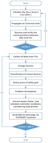
Figure 2. Flowchart of methodology.

4. Proposed Internet of Energy Communication Platform

Constructing an energy-management distributed Internet of Energy (IoE) base is a demanding job. The tasks that the platform must perform are: (1) the integration of the microgrid tools in the communication system and (2) interconnected devices with the IoE cloud for control and monitoring. The proposed IoE communication network consists of four separate layers for carrying out these activities, as depicted in Figure 3. A description of every layer is given below.

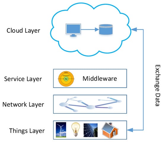
Figure 3. Proposed Internet of Energy platform architecture.

(a)

A things layer that incorporates accessible hardware for controlling/sensing the status of the thing.

(b)

Layer of network that describe the networks and protocols utilized for linking the thing.

(c)

Layer of service producing and handling the resources as necessary. This layer depends on the technology of middleware that offers messaging and routing cover to back run time switching between RR, and publishes and advocates communication patterns to assimilate MG services and features in IoE.

(d)

IoE application cloud layer: The top of the design is this layer, which is responsible for data stowage and analytics. The application layer includes custom MG applications which utilize the data of things.

The HEM has to administer the proposed algorithm by assimilating historical data along with the user input preferences. Hence, a decision has to be made speedily. Furthermore, the state action pair and user inclinations change swiftly during the day and the HEMaaS platform has to offer service in a timely way [53]. Thus, in this study, a Linux based fast microcontroller called Raspberry Pi3 has been utilized. Raspberry Pi3 runs the proposed algorithm by utilizing python programming language.

The web-driven Node-Red programming model has been selected to employ the controlling setup of HEMaaS platforms.

In this research, the BSU and its home appliances communicate via Wi-Fi using a low-power, lightweight, and secure protocol. The MQTT [54] protocol is optimized for a high latency or non-deployable network. MQTT provides network data protection on three levels. It uses a broker in which customers who subscribe to a particular topic publish messages. The topics are described inside the home as a hierarchy of devices [(Room)/(Device)/D1/RaspberryPi]. This pattern was used by the Mosquito [55] broker. The broker supports username and password protection, X.2 certification, and client identifier for HEM network corroboration, and thus intrusion can be prevented. For more details, it is presumed that every microcontroller board of TUs is identified through the single name, and Figure 4 is deployed for the topics.

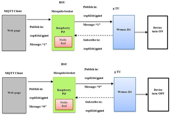
Figure 4. An example for following the information between the web page and TU through BSU.

5. Architecture Proposed Communication

5.1. MQTT Knowledge

The MQTT is the lightweight protocol that uses a network bandwidth with the fixed header of 2 bytes effectively. MQTT operates on the transmission control protocol (TCP) and ensures messages are sent from the node into the server.

There are three key player in MQTT messaging: the MQTT broker, the MQTT publisher, and the MQTT subscriber. The subscriber and publisher of MQTT are not directly connected and are not usually operating concurrently by an IP address. The MQTT Broker is a network gateway that receives, filters, prioritizes, and distributes messages from publishers from up to thousands of simultana-connected MQTT subscribers. The MQTT broker is responsible for customer authorization and the initialization process for communication. For publishing info, MQTT publishers use custom themes to subscribe to clients. MQTT protocol does not allow metadata marking. MQTT topic management can then present metadata for the message load and become considerable in order to attach meaningful attributes to the subject. MQTT is a string with a multi-level, multi-attribute, hierarchical structure. A forward slash in the theme tree separates each stage [56]. These subjects can be updated for routing information. The initialization of connection by exchanging control packet between broker and clients is shown in Figure 5a. The check packets for Link, CONNAC, PUBLISH, PUBACK, SUBACK, SUBSCRIBE, etc., contain specifics of the transmission, theme, and payload quality of service (QoS). The components of the MQTT contact are illustrated in Figure 5b.

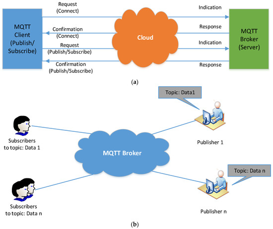
Figure 5. (a) Procedure of protocol MQTT, (b) topic and components of protocol MQTT.

5.2. Proposed Architecture Design Specifications

Figure 6 provides an overview of the proposed hierarchical platform for intelligent building with a physical layer, control layer, and cyber layer. The proposed hybrid platform consists of two communication layers. The smart building devices publish, in their first layer (local layer) for event/measurement reporting, MQTT message to the Building MQTT Clients (BMC), and subscribed for the control/protection intent of BMC published MQTT messages. The second (global) layer consists of BMC-cloud interactions via HTTP POST/GET requests. Each system is fitted with a Wi-Fi module in the proposed architecture, connects to a local portal, and regularly publishes measures on a specially specified theme. The BMC covers all topics and publishes the measurements obtained on a cloud channel. The cloud’s aggregated data can be obtained through the Node-Red cloud interface, which operates an algorithm for the allocation of devices. The algorithm’s results are passed via the BMC from the cloud to the appliances. In the event of a partial communication breakdown in any stage (local or global), the proposed architecture provides resilience. In other words, the BMC is intended to act as a local control (backup controller) for building devices in the event of high network latency or communication connections breakdown. In the results section of this paper, this BMC feature is indicated in a case scenario.

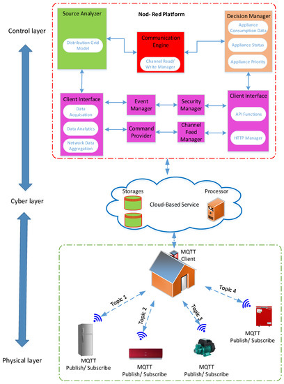
Figure 6. Smart home proposed architecture of communication.

6. Hardware Design of Proposed System

The system hardware comprises one BSU, a wide range of terminal lights (TU), air conditioner, freezer, refrigerator, fans, water level sensors, etc. The following details:

6.1. Base Station Unit

The base station unit (BSU) plays a key part in the proposed system. The BSU hardware comprises a Raspberry Pi3 board. The BSU is in charge of evaluating and diffusing the terminal unit’s data to the web page of the owner. In order to create the Wi-Fi link to which terminals will connect, the BSU needs to be configured in the point of access mode. The Mosquito, an open-source message broker that uses the MQTT protocol, is built in BSU. MQTT provides a lightweight (2 Byte Fixed Header) message management technique using a publishing/subscription model. The internal BSU building for the use of the device is shown in Figure 7.

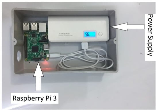
Figure 7. System BSU internal structure.

6.2. The Terminal Units

The Terminal Unit (TU) represents a sub-unit of the wireless sensor network (WSN) setup. Every TU contains a processor, sensor, power module, and wireless communication. TU is a system in charge of gauging water level, current, humidity, temperature, and voltage, as per the sensor content in the node.

The TU controller is a Wemos-D1 board that is in charge of collecting and processing sensor data and conveying acquired information to the BSU. Figure 8 depicts the internal setup of a TU.

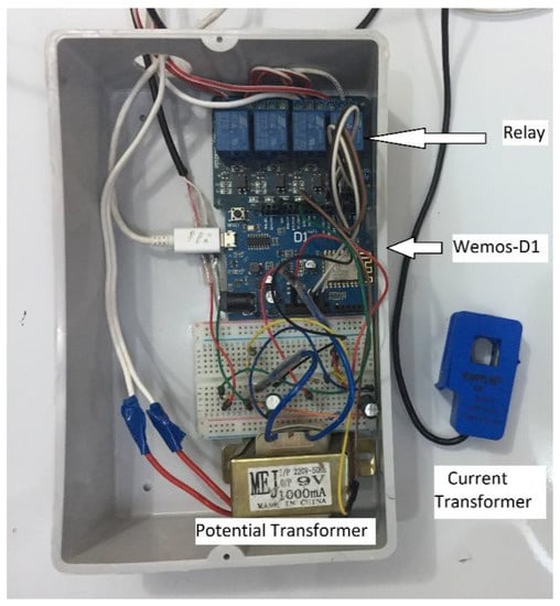
Figure 8. The TU structure of the proposed system.

7. Correction of Power Factor

The ratio of active power (kW) to apparent power (kVA) consumed by an electrical load is known as the power factor (PF) [57]. It may also be understood as ratio of real power use against the total provided power. An inadequate power factor leads to several issues like higher kVA rating of the electricals, higher conductor requirements, relatively ineffective voltage regulation, and higher copper loss, among others. The power factor of a system may be improved using numerous methods like the use of a static capacitor or a synchronous condenser; however, these techniques are either not cost-effective or are inefficient. To overcome these shortcomings, this algorithm based on reactive power was formulated. This algorithm is relatively inexpensive and much more efficient compared to the other techniques. A capacitor is connected to the circuit to have the power factor approach unity to the best possible extent. Capacitor use should be determined based on the reactive power requirement—kVAR. An automatic power factor controller enhances the PF when it falls below a specified threshold. There is a steady increase in energy requirement where both industry and domestic loads are being increasingly inductive. Electrical loads of an inductive nature are the primary reason for a reduced power factor [58]. This section presents a new method to correct the power factor depending on the reactive power method. The mathematical expression for PF is stated in Figure 9.

$$cos\varnothing =\frac{RP}{AP}=PF$$

(18)

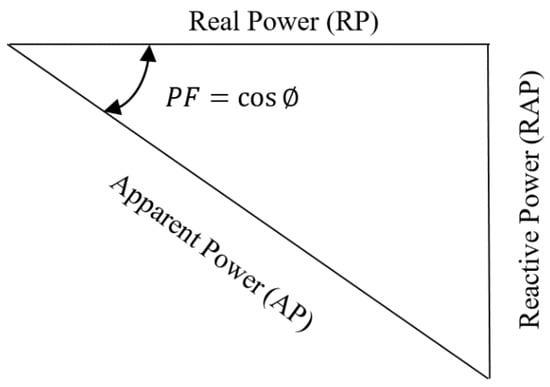
Figure 9. The triangle of power.

The benefits of improving power factor can be defined from the equations below:

$$RP=I\times V\times \cos \varnothing$$

(19)

$$I=\frac{P}{V\times \cos \varnothing }$$

(20)

$$AP=\frac{RP}{\cos \varnothing }$$

(21)

where RP is the Real Power, AP is the Apparent Power, PF is the Power Factor, I is the Current, V is the Voltage, and RAP is the Reactive Power

In the nonsinusoidal system, the Equation (18) changes into Equation (22):

$$PF=\frac{RP}{AP}=\frac{RP}{\sqrt{R{P}^2+RA{P}^2+D^2}}$$

(22)

Even without reactive power, the power factor remains below 1, due to its non-sinusoidal deforming power. The cancelation of reactive power does not necessarily increase the power factor of the sinusoidal device. It is likely that the deformation power will increase further by reducing the reactive power. In non-sinusoidal mode, the power factor can sometimes even worsen if condensers are added [49]:

$$\rho =\frac{RAP}{RP}$$

(23)

$$\tau =\frac{D}{\sqrt{R{P}^2+RA{P}^2}}$$

(24)

Equation (22) turns into Equation (23), where $\cos \zeta$ is a notation given by Equation (26):

$$PF=\frac{RP}{AP}=\frac{RP}{\sqrt{R{P}^2+RA{P}^2}}\times \frac{\sqrt{R{P}^2+RA{P}^2}}{\sqrt{R{P}^2+RA{P}^2+D^2}}=\cos \varnothing \times \cos \zeta$$

(25)

$$\cos \zeta =\frac{\sqrt{R{P}^2+RA{P}^2}}{\sqrt{R{P}^2+RA{P}^2+D^2}}<1$$

(26)

The power factor expression is rewritable as Equation (27):

$$PF=\frac{1}{\sqrt{1+{\rho }^2}}\times \frac{1}{\sqrt{1+{\tau }^2}}$$

(27)

The definition of the power factor in a non-sinusoidal system does not express the degree of power used available in network, as harmonic sources are not the network generators, but non-linear receivers.

Two power factor values have been described and calculated in the non-sinusoidal mode: the power factor for the basic component (fundamental 50/60 Hz or DPF) and the total PF (true/total power factor):

$$DPF=\cos {\varnothing }_1=\frac{R{P}_1}{A{P}_1}$$

(28)

$$PF=\frac{RP}{AP}=\frac{RP}{I\times V}$$

(29)

The total power factor involves the effect of harmonics on apparent power and active power offers information on how effectively the active power is used by the client.

Depending on current and voltage distortions variables, an expression may be defined for total power factor in a non-sinusoidal system. To do this, there are written expressions of apparent power and active power. The active power in the non-sinusoidal system is generated by the number of active powers, which each partly coincide with each harmonic, producing two parts, the fundamental active power and a harmonic active power [49].

$$RP={\displaystyle \sum }_{h=1}{I}_h\times V_h\times \cos \left({\propto }_h-{\beta }_h\right)={\displaystyle \sum }_{h=1}{I}_h\times V_h\times \cos {\varnothing }_h=P_1+P_h$$

(30)

$$R{P}_1=I_1\times V_1\times \cos {\varnothing }_1$$

(31)

$$R{P}_h={\displaystyle \sum }_{h=1}{I}_h\times V_h\times \cos {\varnothing }_h$$

(32)

The apparent power of an electrical dipole is defined by the voltage and current RMS value, as AP in Equation (33) is indicated. Similarly, the apparent power of the non-sinusoidal system is capable of decomposing itself into the fundamental apparent power of Equation AP1 (34) and Equation (35) harmonic apparent (residual apparent) power of SN. The key obvious power—AP1 and its RP1 and RAP1 components—is of great concern, since they interfere in the circuit’s circulation of power. The apparent power can be expressed in the non-sinusoidal mode in accordance with the voltage RMS and the current RMS values accordingly in Equation (36):

$$AP=V\times I$$

(33)

$$A{P}_1=V_1\times I_1$$

(34)

$$A{P}_1^2=R{P}_1^2+RA{P}_1^2$$

(35)

$$A{P}^2={\left(I\times V\right)}^2=\left(V_1^2+V_h^2\right)\times \left(I_1^2+I_h^2\right)=S_1^2+S_h^2$$

(36)

$$k_{d1}=TH{D}_I=\frac{I_h}{I_1}=\sqrt{\frac{{{\displaystyle \sum }}_{h\ne 1}{I}_h^2}{I_1^2}},k_{dV}=TH{D}_V=\frac{V_h}{V_1}=\sqrt{\frac{{{\displaystyle \sum }}_{h\ne 1}{V}_h^2}{V_1^2}}$$

(37)

where (THDV) is total harmonic distortion factor for voltage and (THDI) is the total harmonic distortion factor for current, both defined below:

$$PF=\frac{RP}{AP}=\frac{R{P}_1+R{P}_h}{\sqrt{A{P}_1^2+A{P}_N^2}}=\frac{\frac{R{P}_1}{A{P}_1}\times \left(1+\frac{R{P}_h}{R{P}_1}\right)\times DPF}{\sqrt{1+{\left(\frac{A{P}_N}{A{P}_1}\right)}^2}}=\frac{\left(1+\frac{R{P}_h}{R{P}_1}\right)\times DPF}{\sqrt{1+TH{D}_I^2+TH{D}_V^2+{\left(TH{D}_I+TH{D}_V\right)}^2}}$$

(38)

For $TH{D}_I>40\%$ and $TH{D}_V<5\%$, the Equation (39) shows the relation between fundamental power factor and total power factor:

$$PF=\frac{1}{\sqrt{1+TH{D}_I^2}}\times DPF=\frac{I_1}{I}\times \cos {\varnothing }_1$$

(39)

The power factor fundamental is nearly at 1, but the overall power factor can be 0.5–0.6 for certain modern devices such as switching power supplies or speed changing equipment. The power factor fundamental and total power factor must be calculated in order to prevent non-compliant situations [49].

Equation (40) shows the arithmetic apparent power:

$$A{P}_a={\displaystyle \sum }_{x\in A,B,C}A{P}_x=A{P}_A+A{P}_B+A{P}_C={\displaystyle \sum }_{x\in A,B,C}\sqrt{R{P}_x^2+RA{P}_x^2}$$

(40)

where, $A{P}_{A,B,C}$, $R{P}_{A,B,C}$, and$RA{P}_{A,B,C}$, show active power, apparent power, and reactive power on a phase.

Geometrical apparent power can be written as:

$$A{P}_g=\sqrt{R{P}^2+RA{P}^2}$$

(41)

$$RP={\displaystyle \sum }_{x\in A,B,C}R{P}_x=R{P}_A+R{P}_B+R{P}_C$$

(42)

$$RAP={\displaystyle \sum }_{x\in A,B,C}RA{P}_x=RA{P}_A+RA{P}_B+RA{P}_C$$

(43)

However, it can also be written in the form of Equation (44):

$$A{P}_g=\left|R{P}_A+R{P}_B+R{P}_C+j\times \left(RA{P}_A+RA{P}_B+RA{P}_C\right)\right|=\left|RP+j\times RAP\right|$$

(44)

$$P{F}_a=\frac{RP}{A{P}_a}=\frac{R{P}_A+R{P}_B+R{P}_C}{A{P}_A+A{P}_B+A{P}_C}$$

(45)

$$P{F}_g=\frac{RP}{A{P}_g}=\frac{R{P}_A+R{P}_B+R{P}_C}{\left|\underset{\_}{A{P}_A}+\underset{\_}{A{P}_B}+\underset{\_}{A{P}_C}\right|}$$

(46)

where,

$$\underset{\_}{A{P}_A}=R{P}_A+j\times RA{P}_A;\underset{\_}{A{P}_B}=R{P}_B+j\times RA{P}_B;\underset{\_}{A{P}_C}=R{P}_C+j\times RA{P}_C$$

(47)

$$RA{P}_A=\sqrt{R{P}_A^2+RA{P}_A^2+D_A^2};RA{P}_B=\sqrt{R{P}_B^2+RA{P}_B^2+D_B^2};RA{P}_C=\sqrt{R{P}_C^2+RA{P}_C^2+D_C^2}$$

(48)

The apparent arithmetic power is:

$$A{P}_a=A{P}_A+A{P}_B+A{P}_C$$

(49)

where geometrical apparent power is given in (48), and its components are given in (49):

$$A{P}_g=\sqrt{R{P}^2+RA{P}^2+D^2}$$

(50)

$$RP=R{P}_A+R{P}_B+R{P}_C,RAP=RA{P}_A+RA{P}_B+RA{P}_C,D=D_A+D_B+D_C$$

(51)

The term equal apparent power is used to describe an apparent intensity in the case of an unbalanced load. In the same way as we have an obvious capacity for balance loads, this is connected to losses in power lines and transformers. Compared to Equation (52), an equivalent current $I_e$ and an equivalent phase voltage $V_e$ can be defined in Equation (53):

$$AP=\sqrt{3}\times V\times I$$

(52)

$$A{P}_e=\sqrt{3}\times V_e\times I_e$$

(53)

The equivalent voltage is given by Equation (54) for a three phase circuit with a neutral conductor:

$$V_e=\sqrt{\frac{V_a^2+V_b^2+V_c^2}{3}}$$

(54)

The equivalent voltage can be calculated with Equation (55) for a three-phase circuit without a neutral conductor:

$$V_e=\sqrt{\frac{V_{AB}^2+V_{BC}^2+V_{CA}^2}{9}}$$

(55)

The RMS value of the equivalent current is evaluated according to the RMS values of the currents, $I_A$, $I_B$, and $I_C$ in Equation (56):

$$I_e=\sqrt{\frac{I_A^2+I_B^2+I_C^2}{3}}$$

(56)

For the particular case of a balanced and linear load, we have $V_e$ = V, $I_e=I_A=I_B=I_C$, and the apparent power is written according to Equation (57):

$$A{P}_e=AP=\sqrt{3}\times V\times I$$

(57)

Equivalent power-factor results in Equation (58):

$$P{F}_e=\frac{RP}{A{P}_e}$$

(58)

The automated power factor correction (APFC) system proposed in the study relies on a microcontroller-based system to control capacitor control. This work uses a system comprising of three capacitors for the APFC system, and a series connection between the microcontroller and the capacitors. The intent is to have the microcontroller determine the system PF, voltage, and current levels. Subsequently, the microcontroller should compute the number of capacitors required to achieve the desired power factor level. The primary components comprising the system are capacitors, microcontroller, interfacing devices (voltage, current, and PF), contactors, and relays.

The system uses a 220 V supply and uses a potential transformer (PT) to step down the voltage to 9 V and then the AC supply is converted to less than 5 volts to provide a signal appropriate for the microcontroller. A current transformer (CT) is attached to the load to determine the current. The CT output is fed to the current sensing circuit, and the output feeds to the analogue input of the microcontroller. Subsequently, the microcontroller computes the PF and switches the capacitors required for the circuit. Circuit parameters like voltage, current, apparent power, and real power are shown on a web page. The schematic of proposed APFC system is illustrated in Figure 10.

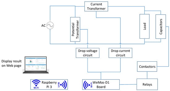
Figure 10. The proposed APFC diagram.

7.1. Voltage Measurement

The potential transformer (PT), as depicted in Figure 11b, converts the 220 V input to 9 V. Since the microcontroller accepts an analogue input in the 0–5 V range, it is essential to step down the 9 V output of the transformer in this range.

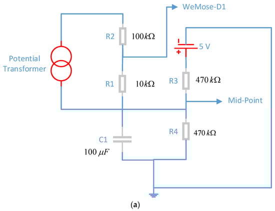
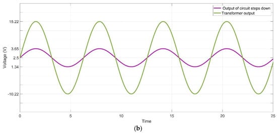
Figure 11. (a) Step down voltage circuit diagram, (b) the input and output signal of the circuit diagram.

The RMS voltage reading is required to determine the apparent and real power values and, therefore, the power factor. An AC/AC power transformer may be utilized for this purpose. The transformer steps down the high voltage, and then a conditioning circuit is employed to adapt the PT output signal. The positive peak value for a 9 V signal is +12.727 V, while the negative peak is −12.727 V. The conditioning circuit should be able to change the transformer output within a 0–5 V signal range, i.e., the positive peak should not exceed 5 volts, while the negative peak should be higher than 0 volts.

The PT output waveform is sinusoidal, and a voltage divider attached across the transformer terminals is used to scale down the voltage. Furthermore, the signal shift is achieved using the addition of one more voltage divider connected to the power source of the microcontroller. The output should be in the 0 V to 5 V reference range required for the analogue-to-digital converter (ADC). The circuit diagram for the voltage sensing circuit is depicted in Figure 11.

The PT output is scaled using the two resistors R1 and R2 that form the voltage divider. The circuit output is smoothened using C1, which removes the ripples from the output. The 2.5 V signal is achieved across R3 and R4, which act as voltage dividers.

$$\begin{gathered} POV = \frac{ R1}{\left(R2 + R1\right)} \times PIV \\ = \frac{10k}{\left(10k+100k\right)}\times 12.72= 1.156\mathrm{V} \end{gathered}$$

(59)

where POV is the peak output voltage, PIV is the peak input voltage

$$\begin{gathered} PPV=2\times POV \\ =2\times 1.156=2.312 \mathrm{V} \end{gathered}$$

(60)

where PPV is the peak to peak voltage.

Resistors R3 and R4 had a resistance of 470 k ohm and facilitated the voltage signal shift. The other microcontroller also uses a supply of 5 V, and the resulting sinusoidal waveform is

$$\begin{gathered} Positive peak = \frac{RMV}{2} + \frac{PPV}{2} \\ = \frac{5}{2}+\frac{2.312}{2}=3.656 \mathrm{V} \end{gathered}$$

(61)

where RMV is the reference microcontroller voltage

$$\begin{gathered} Negative peak = \frac{RMV}{2}- \frac{PPV}{2} \\ = \frac{5}{2}-\frac{2.312}{2}=1.344 \mathrm{V} \end{gathered}$$

(62)

Using Equations (61) and (62), it can be seen that the positive peak voltage is 3.65 V, while the negative peak is 1.344 V, both of which are in the acceptable voltage range of the microcontroller.

7.2. Current Measurement

Using a current transformer with microcontrollers requires current transformer output to be scaled so that the signal is in the acceptable range for microcontroller input. The current sensing circuit diagram is depicted in Figure 12.

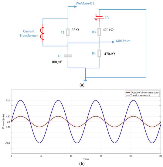
Figure 12. (a) Step down current circuit diagram, (b) current sensing circuit diagram.

Resistance computation requires the CT signal to provide a signal that crosses the resistor. Since the maximum current is 100 A, the same value is selected as the CT current. The peak value of current is specified as:

$$\begin{gathered} PPI = \sqrt{2}\times I \\ =1.41\times 100=141 A \end{gathered}$$

(63)

where PPI is the primary peak current and I is the RMS current

Furthermore, the secondary coil peak current is given by:

$$\begin{gathered} SPI = \frac{PPI}{N} \\ =\frac{141}{2000}=70 \mathrm{mA} \end{gathered}$$

(64)

where SPI is the secondary peak current and N is the number of turns.

The load resistor should have a voltage value equivalent to half of the microcontroller’s reference voltage while functioning under a peak current to increase voltage resolution.

$$\begin{gathered} BR= \frac{\frac{RMV}{2}}{SPI} \\ = 2.5\mathrm{V}/0.0707\mathrm{A} = 35.36 \mathsf{\Omega } \end{gathered}$$

(65)

where BR is the burden resistance.

The value of the burden resistance is kept at 33 Ω (and not 35.36 Ω), since that value is not available on a standard resistor.

$$\begin{gathered} PCTO = \sqrt{2}\times I \\ =\sqrt{2}\times 50\mathrm{mA}=70.71\mathrm{mA} \end{gathered}$$

(66)

where PCTO is the peak current transformer output

$$\begin{gathered} PPCTO=2 \times PCTO \\ = 2\times 70.71\mathrm{mA}=141.42\mathrm{mA} \end{gathered}$$

(67)

where PPCTO is the peak to peak current transformer output

$$\begin{gathered} PPV = PPCTO\times BR \\ =141.42\mathrm{mA}\times 33\Omega =4.66\mathrm{V} \end{gathered}$$

(68)

The voltage, as measured between the peaks, is 4.66 V, which is in the operational range of the microcontroller. The voltage ripples in the output are eliminated using a capacitor ($C_1$), and the output waveform is smoother. Resistors ($R_3$) and ($R_4$) form the voltage divider that is used to get the 2.5 V signal. The microcontroller has an operational voltage of 5 V, and the sinusoidal waveform has negative and positive peaks. The positive peak may be calculated using Equation (61):

$$Positive peak=\frac{5}{2}+ \frac{4.66}{2}=4.83 \mathrm{V}$$

The negative peak is determined with Equation (62) as:

$$Negative peak=\frac{5}{2}-\frac{4.66}{2}=0.16 \mathrm{V}$$

The positive voltage peak has a value of 4.83 V, while the negative peak stands at 0.16 V, both of which are in the operational range of the microcontroller input.

7.3. Capacitor Bank

The capacitor bank comprises multiple capacitors having different capacitance values. The shunt connection provided between the capacitors provided the adequate value required for correcting the power factor. The reactive power load is a determinant of the capacitance requirement. The proposed system had capacitors having 5 µF, 10 µF, and 20 µF capacitance. Figure 13 shows complete APFC and energy monitoring system.

$$RAP= \sqrt{{\left(AP\right)}^2-{\left(RP\right)}^2}$$

(69)

where RAP is reactive power in VAR, AP is apparent power in VA, and RP is real power in kW

$$C = \left(RP/2\pi f V^2\right)$$

(70)

where C is the capacitance in Farad

$$RAP = V^2\times 2\pi fC$$

(71)

where V is a voltage, and $f$ is power system frequency.

$$Reactive power of 20 \mathsf{\mu }\mathrm{F}=5\times {10}^{-6}\times 50\times 2\times 20\times 3.14\times {220}^2=304 VAR$$

$$Reactive power of 10 \mathsf{\mu }\mathrm{F}=5\times {10}^{-6}\times 50\times 2\times 10\times 3.14\times {220}^2=152 VAR$$

$$Reactive power of 5 \mathsf{\mu }\mathrm{F}=5\times {10}^{-6}\times 50\times 2\times 5\times 3.14\times {220}^2=76 VAR$$

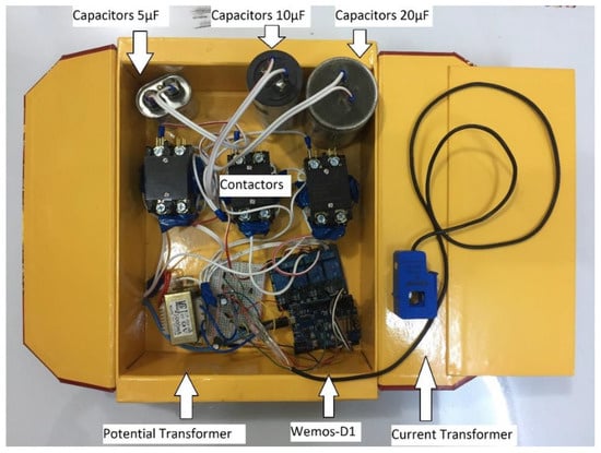
Figure 13. Complete APFC and energy monitoring system.

8. Automatic Protective System Manager

The design of the automatic protective system manager for a smart home is such that it can safeguard television, lamps, fans, refrigerator, and other home appliances from excess current, excess voltage, or drop in voltage situations. The fundamental benefit of such a system is that it can add automatic functionality to turn on and turn off appliances independently based on certain pre-determined criteria and priorities related to over-current, over-voltage, and under voltage. There is a mechanism in the system to make comparisons between actual and set values of voltage and current. The controller is designed to send the trip signal to the intended device whenever these values exceed the threshold values. In this study, the current and voltage values have been between the limits.

$$V<V_{Min} or V>V_{Max}$$

(72)

$$V_{Min}<V<V_{Max}$$

(73)

$$I<I_{Min}, I>I_{Max}$$

(74)

where $V_{Min}$ is minimum voltage, $V_{Max}$ is maximum voltage, $I_{Min}$ is minimum current, and $I_{Max}$ is maximum current.

9. Experimental Results

To experiment and demonstrate the advantages of HEMS over a cloud as a service (HEMaaS), numerous services have been evaluated and implemented over the platform.

In this section, the outcomes of smart energy management as a service implemented with the suggested algorithm over a cloud platform to regulate appliances in a sample smart home have been presented and discussed. As elaborated in the software communication and architecture interface, there is a Raspberry-Pi3 in the main command and control unit (MCCU) organizing the Node-Red platforms. MQTT (Mosquitto) functions as a broker between subscribing home appliances and the MCCU publisher. In order to regulate the home appliances through a MQTT gateway, custom python code using proposed algorithm has been deployed on it, which runs on Raspberry Pi3. In this work, the Node-Red dashboard interface that has been designed is a simple and convenient user interface (UI) that enables a homeowner to access and interact with HEMS over a cloud as a service system. Figure 14 shows the dashboard control and the UI flow design.

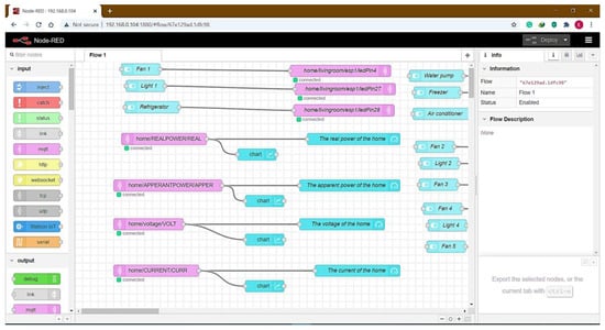
Figure 14. User interface design platform (Node-Red platform).

During the demand response (DR) event, there are certain challenges with regards to attaining the most optimal or the best schedule for house devices, so that customer loads can be switched to reduce cost of electric power consumption through the proposed rules. As a result, specific advanced optimization procedures are needed to schedule house devices. An optimal schedule controller constitutes of three sub-components that include an optimization technique, schedule condition of customer, and design of suggested schedule controller. Based on appliance priority and customer comfort preference, each appliance is compared against a number of set points, which include power consumption, load priority, and customer preference setting on the water level of tank or the room temperature of air conditioner. Table 1 presents the load priority and the homeowner preference settings. Figure 15 demonstrates the flow of schedule controller conditions in terms of the house devices. In initial stages, data is read from all the connected devices. Thereafter, as shown in Table 1, each appliance is compared against a range of set points. If the overall power consumption is greater than the demand limit (DL), the system algorithm will turn OFF an appliance with the lowest priority starting with REF. The algorithm would further compel the loads to shift their operating time to maintain total power consumption under DL after the DR interval has elapsed.

Table 1. Characteristics of load priority and power ratings.

Devices	Priority Load	Effected by under Voltage	Effected by over Voltage	Priority According Current	Customer Comfortable Lifestyle	Max Number
Refrigerator	1	yes	yes	Maybe	24 h	1
Water pump	2	yes	yes	Maybe	Maybe	1
Freezer	3	yes	yes	Maybe	24 h	1
Fluorescent Light	4	no	no	Maybe	Maybe	15
Fan	5	no	no	No	24 h	6
Air conditioner	6	yes	yes	Yes	Temperature of room 23–26	1

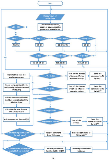
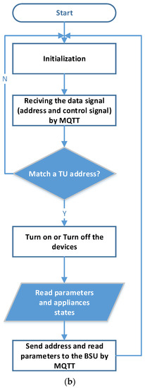
Figure 15. Diagram of the time limit for load priority controls, (a) BSU flowchart, (b) TU flowchart.

9.1. The Protocol of the Proposed System

After the software starts operating, the BSU receives a command from a web page, and it is forwarded by the BSU to a TU with an address. All TUs receive addresses from BSU. When the TU address matches the address received from the BSU, then it will interact with received message and execute the command present in the message. Each TU passes the specified parameters in a message and sends these parameters to the BSU with their address. The BSU passes these data to the web page after receiving sensed data from all TUs. The flowchart of the proposed BSU webpage structure is illustrated in Figure 15a. The TU flowchart is also shown in Figure 15b.

9.2. Access of Internet Web Page

In order to access the web page locally, the internet protocol (IP) used is Raspberry Pi3 IP local ports 1880 dedicated to the web-page Node-Red. The local IP is http://192.168.0.104:1880/ui. Ngrok helps convert the Raspberry Pi3 local IP address to a global IP address for page access through the internet from anywhere in the world. The web page http:/4a652641cd68.ngrok.io is accessible during Ngrok’s registration for the web page. Figure 16 shows the internet webpage in any browser, after entering and providing the username and password in the uniform resource locator (URL).

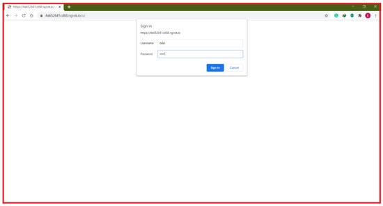
Figure 16. Web site and prompt to enter username and password after entering the URL in the browser.

9.3. Result without Corrective Method

The HEMS comprises the GUI (graphical user interface) and related software to facilitate customers in examining individual and total cost, power consumption, voltage, and current of the home appliances; their power factor and apparent power before the proposed algorithm is implemented as displayed in Figure 17. Moreover, every home appliance can also be turned on/off manually using a push button switch available in interface of the dashboard.

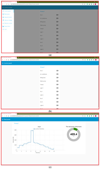
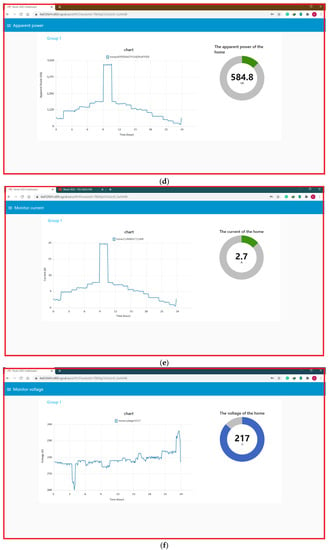
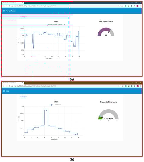
Figure 17. Graphical user interface of proposed HEMS before implementing the proposed algorithm, (a) main page, (b) control panel, (c) real power consumption, (d) apparent power consumption, (e) current of home loads, (f) voltage of home load, (g) power factor of loads, and (h) the cost.

The information regarding power consumption is collected in real time for 24 h without the controllers at week days in Iraq. In the case of the weekdays, the individual and the total power consumption of all the home appliances including light, water pump, refrigerator, and air conditioning system have been obtained from HEMS without use of a schedule controller as displayed in Figure 17. The proposed schedule controller that is proposed is used to decrease energy during DR events, taking into consideration many devices per hour for the weekdays.

The total consumption of real power is found to be 277.428 kWh in the case of weekdays. The total consumption of apparent power is found to be 305.416 kWh in the case of weekdays. Additionally, in Iraq, the price is $0.067 per kW/h, and the total cost is found to be $18.5877035 in the case of weekdays. The home appliance performance for energy saving is considered significant for developing better groundwork that can be used by customer.

Furthermore, every home appliance’s performance can be conveniently changed as per the requirement of the customer; for instance, the refrigerator and the air conditioning system function for 24 h on weekdays. To validate the established controller, the proposed schedule controller is compared with no schedule controller. The Appendix A contains details and data of the nanogrid before implementing the proposed correction method

9.4. Result with Corrective Method

Real data representing a residential sector in Iraq were collected to demonstrate the efficiency of the proposed algorithms. The total consumption of real power after applying the proposed algorithm is found to be 271.081 kWh in the case of weekdays. The total consumption of apparent power after applying the proposed algorithm is found to be 298.134 kWh in the case of weekdays. In Iraq, the price is $0.067 per kW/h, and the total cost after applying the proposed algorithm is found to be $16.2648647 in the case of weekdays.

Figure 18 displays the results in the case of weekdays obtained by using developed schedule controller at different time of day. In Figure 18, the proposed HEMS schedule controller can be observed. The outcomes of the schedule controller proposed in this study can significantly lessen peak hour consumption of energy on the weekdays during the DR, whose value amounts to 271.081 kWh per day. Additionally, the outcomes of the developed schedule controller can decrease the energy usage cost as well as correct the power factor value of the home loads.

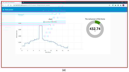
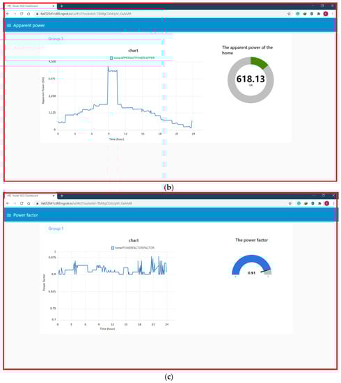
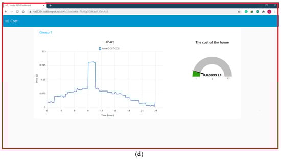
Figure 18. Graphical user interface of the proposed HEMS after implementing proposed algorithm, (a) real power consumption, (b) apparent power consumption, (c) power factor of loads, and (d) the cost.

This Appendix B contains details and data of the nanogrid after implementing the proposed correction method.

10. Discussion

The performance of microgrid communication and control system under various operation modes is investigated. The poor performance of the system of control is due to the limitation of MQTT TCP/IP in distributed communication mode. The MQTT communication protocol is suitable for applications with a simple structure and high data transmission. With the distributed communication system, it can be seen that the optimization system of the microgrid reduces the operating costs. The information regarding power consumption is collected in real time for 24 h without the controllers on weekdays in Iraq. In the case of the weekdays, the individual and total power consumption of all the home appliances including light, water pumps, refrigerators, and air conditioning systems have been obtained from the home energy management system without use of schedule controller. Before applying the proposed algorithm, the total consumption of real power was found to be 277.428 kWh in the case of wee days. The total consumption of apparent power before applying the proposed algorithm is found to be 305.416 kWh in the case of weekdays. The price before applying the proposed algorithm is $0.067 per kW/h, and the total cost is found to be $18.5877035 in the case of weekdays.

After applying the proposed algorithm, the total consumption of real power is found to be 271.081 kWh in the case of week days. The total consumption of apparent power after applying the proposed algorithm is found to be 298.134 kWh in the case of weekdays. In Iraq, the price is $0.067 per kW/h, and the total cost after applying the proposed algorithm is found to be $16.2648647 in the case of weekdays. By comparing applying the proposed algorithm with the traditional algorithm approximately, the schedule controller proposed in this paper achieved an energy saving of 6.347 kWh real power per day, this paper achieved saving 7.282 kWh apparent power per day, and the proposed algorithm in our paper saved $2.3228388 per day.

11. Conclusions

In this study, we have proposed a novel smart energy management employed as a service over the cloud computing platform. This study has presented the implementation of a cloud-based communication platform for appliance-level in smart neighborhood areas with the utility grid. The use of the platform of cloud computing provides the connectivity, interoperability, flexibility, and data privacy, as well as the real-time features essential for energy management. This study is the major contribution to the literature on smart home functioning and it proposes RTES (real-time electricity scheduling) for HEMS, which considers the errors of information prediction. Unlike the majority of the earlier HEMS approaches that revolve around DAES (day-ahead electricity scheduling), we proposed a real-time scheduling system that makes sure that the scheduling of every period is the soundest decision based on information prediction within the upcoming 24 h. The proposed algorithm has a hierarchical architecture with local and global communication layers based on MQTT and HTTP TCP/IP protocols for cloud interactions. The wireless communication (Wi-Fi) is set up between the TUs and the BSU controller. It is also integrated with a novel advanced self-diagnostic system to form a reliable network. Experimental results show that the RTES system gives better performance compared to DAES in terms of total electricity cost payment, and the HEMS integrated with RTES approach can quickly act when there is a sudden variation in the system inputs. The schedule controller proposed in this paper achieved an energy saving of 6.347 kWh real power per day, this paper achieved saving 7.282 kWh apparent power per day, and the proposed algorithm in our paper saved $2.3228388 per day.

The newly designed closed-loop adaptive power factor controller proposed in this paper is a very effective device to compensate for the reactive power of rapidly varying loads. The device has a large number of features that make it very promising for a wide range of industrial applications. The new design ensures the best possible compensation even when some of the switching circuit components fail. The results of the field test, so far, show that the device can provide almost unity (equal 1) power factor at the point of installation regardless of the dynamic variation of the load reactive power. Another advantage of the proposed device was that it could observe and regulate power factor correction distantly using an internet connection from anywhere in the world, enabling easy fine-tuning of the control parameters of the algorithm to possibly obtain better functioning.

Lastly, in order to access the data regarding power consumption of individual load, a reliable web portal related to an IoT environment is created. A graphical user interface (GUI) is provided with plotting of power consumption to examine every appliance’s power usage on daily basis and, further, a database is also provided for energy management, which can also be used for further analysis of the data.

The proposed algorithm results were compared with the previous schedule controller, and the presented results show that the proposed algorithm schedule controller is better than the previousw algorithm. Where the total consumption before is applied, the proposed algorithm found that real power is 277.428 kWh, apparent power is found to be 305.416 kWh, and total cost is found to be $185,877,035 in the case of weekdays. However, the total consumption of real power after applying the proposed algorithm is found to be 271.081 kWh, apparent power is found to be 298.134 kWh, and the total cost after is found to be $16.2648647 in the case of weekdays. From comparing applying the proposed algorithm with previous works, the proposed algorithm in this paper achieved an energy saving of 6.347 kWh real power per day, and saved 7.282 kWh apparent power per day, and the proposed algorithm in our paper saved $2.3228388 per day.

The results revealed that the proposed schedule controller performs better in minimizing the energy consumed by household devices during weekdays, and the power factor is improved. The results indicated that the proposed home energy management system is effective. In addition, the model can control the devices and keep total consumption of residential energy below the given demand limit.

Future extension of this work may include the integration of the LoRaWAN network with the proposed IoT architecture, because the use of the LoRaWAN technology could lead to a very promising solution, due to its good coverage capabilities (both in outdoor and in hybrid environments), whereas its most critical aspect is represented by the relatively low data throughput and duty cycle limitation.

References

- Wang, Y.; Nguyen, T.L.; Syed, M.H.; Xu, Y.; Guillo-Sansano, E.; Burt, G.; Tran, Q.T.; Caire, R. A Distributed Control Scheme of Microgrids in Energy Internet Paradigm and Its Multi-Site Implementation. IEEE Trans. Ind. Inform. 2020. [Google Scholar] [CrossRef]
- Zou, H.; Wang, Y.; Mao, S.; Zhang, F.; Chen, X. Distributed Online Energy Management in Interconnected Microgrids. IEEE Internet Things J. 2020, 7, 2738–2750. [Google Scholar] [CrossRef]
- Li, S.; Yang, J.; Song, W.; Chen, A. A Real-Time Electricity Scheduling for Residential Home Energy Management. IEEE Internet Things J. 2019, 6, 2602–2611. [Google Scholar] [CrossRef]
- Tajalli, S.Z.; Mardaneh, M.; Taherian-Fard, E.; Izadian, A.; Kavousi-Fard, A.; Dabbaghjamanesh, M.; Niknam, T. DoS-Resilient Distributed Optimal Scheduling in a Fog Supporting IIoT-Based Smart Microgrid. IEEE Trans. Ind. Appl. 2020, 56, 2968–2977. [Google Scholar] [CrossRef]
- Chen, Y.Y.; Lin, Y.H.; Kung, C.C.; Chung, M.H.; Yen, I. Design and Implementation of Cloud Analytics-Assisted Smart Power Meters Considering Advanced Artificial Intelligence as Edge Analytics in Demand-Side Management for Smart Homes. Sensors 2019, 19, 2047. [Google Scholar] [CrossRef] [PubMed]
- Naji Alhasnawi, B.; Jasim, B.H.; Esteban, M.D. A New Robust Energy Management and Control Strategy for a Hybrid Microgrid System Based on Green Energy. Sustainability 2020, 12, 5724. [Google Scholar] [CrossRef]
- Alhasnawi, B.N.; Jasim, B.H. Internet of Things (IoT) for Smart Grids: A Comprehensive Review. J. Xi’an Univ. Archit. 2020, 63, 1006–7930. [Google Scholar]
- Khalid, A.; Aslam, S.; Aurangzeb, K.; Haider, S.I.; Ashraf, M.; Javaid, N. An Efficient Energy Management Approach Using Fog-as-a-Service for Sharing Economy in a Smart Grid. Energies 2018, 11, 3500. [Google Scholar] [CrossRef]
- Bedi, G.; Venayagamoorthy, G.K.; Singh, R.; Brooks, R.; Wang, K.C. Review of internet of things (IoT) in electric power and energy systems. IEEE Internet Things J. 2019, 5, 847–870. [Google Scholar] [CrossRef]
- Al-Ali, A.R.; Zualkernan, I.A.; Rashid, M.; Gupta, R.; Alikarar, M. A Smart Home Energy Management System Using IoT and Big Data Analytics Approach. IEEE Trans. Consum. Electron. 2017, 63, 426–434. [Google Scholar] [CrossRef]
- La Tona, G.; Luna, M.; Di Piazza, A.; Di Piazza, M.C. Towards the Real-World Deployment of a Smart Home EMS: A DP Implementation on the Raspberry Pi. Appl. Sci. 2019, 9, 2120. [Google Scholar] [CrossRef]
- Soares, A.; Gomes, A.; Antunes, C.H.; Oliveira, C. A Customized Evolutionary Algorithm for Multiobjective Management of Residential Energy Resources. IEEE Trans. Ind. Inform. 2017, 13, 492–501. [Google Scholar] [CrossRef]
- Paterakis, N.G.; Erdinç, O.; Bakirtzis, A.G.; Catalão, J.P.S. Optimal household appliances scheduling under day-ahead pricing and load-shaping demand response strategies. IEEE Trans. Ind. Inform. 2015, 11, 1509–1519. [Google Scholar] [CrossRef]
- Nambi, S.N.A.U.; Pournaras, E.; Venkatesha Prasad, R. Temporal Self-Regulation of Energy Demand. IEEE Trans. Ind. Inform. 2016, 12, 1196–1205. [Google Scholar] [CrossRef]
- Palensky, P.; Dietrich, D. Demand side management: Demand response, intelligent energy systems, and smart loads. IEEE Trans. Ind. Inform. 2011, 7, 381–388. [Google Scholar] [CrossRef]
- Nunna, K.H.S.V.S.; Doolla, S. Responsive End-User based Demand Side Management in Multi-Microgrid Environment. IEEE Trans. Ind. Inform. 2014, 10, 1262–1272. [Google Scholar] [CrossRef]
- Nadeem, Z.; Javaid, N.; Malik, A.W.; Iqbal, S. Scheduling Appliances with GA, TLBO, FA, OSR and Their Hybrids Using Chance Constrained Optimization for Smart Homes. Energies 2018, 11, 888. [Google Scholar] [CrossRef]
- Khalid, A.; Javaid, N.; Mateen, A.; Khalid, B.; Khan, Z.A.; Qasim, U. Demand Side Management using Hybrid Bacterial Foraging and Genetic Algorithm Optimization Techniques. In Proceedings of the 2016 10th International Conference on Complex, Intelligent, and Software Intensive Systems (CISIS), Fukuoka, Japan, 6–8 July 2016; IEEE: Piscataway, NJ, USA, 2016; pp. 494–502. [Google Scholar]
- Yan, C.; Xue, X.; Wang, S.; Cui, B. A novel air-conditioning system for proactive power demand response to smart grid. Energy Convers. Manag. 2015, 102, 239–246. [Google Scholar] [CrossRef]
- Keshtkar, A.; Arzanpour, S. A fuzzy logic system for demand-side load management in residential buildings. In Proceedings of the 2014 IEEE 27th Canadian Conference on Electrical and Computer Engineering (CCECE), Toronto, ON, Canada, 4–7 May 2014; IEEE: Piscataway, NJ, USA, 2014; p. 15. [Google Scholar]
- Liu, Y.; Yuen, C.; Yu, R.; Zhang, Y.; Xie, S. Queuing-based energy consumption management for heterogeneous residential demands in smart grid. IEEE Trans. Smart Grid 2016, 7, 1650–1659. [Google Scholar] [CrossRef]
- Ma, J.; Chen, H.H.; Song, L.; Li, Y. Residential load scheduling in smart grid: A cost-efficiency perspective. IEEE Trans. Smart Grid 2016, 7, 771–784. [Google Scholar] [CrossRef]
- Shirazi, E.; Jadid, S. Optimal residential appliance scheduling under dynamic pricing scheme via HEMDAS. Energy Build. 2015, 93, 40–49. [Google Scholar] [CrossRef]
- Khalid, A.; Javaid, N.; Mateen, A.; Ilahi, M.; Saba, T.; Rehman, A. Enhanced Time-of-Use Electricity Price Rate Using Game Theory. Electronics 2019, 8, 48. [Google Scholar] [CrossRef]
- Wang, J.; Liu, F.; Song, Y.; Zhao, J. A novel model: Dynamic choice articial neural network (DCANN) for an electricity price forecasting system. Appl. Soft Comput. 2016, 48, 281–297. [Google Scholar] [CrossRef]
- Zhou, L.; Wu, D.; Chen, J.; Dong, Z. Greening the smart cities: Energy-efficient massive content delivery via D2D communications. IEEE Trans. Ind. Inform. 2018, 14, 1626–1634. [Google Scholar] [CrossRef]
- Mengelkamp, E.; Notheisen, B.; Beer, C.; Dauer, D.; Weinhardt, C. A blockchain-based smart grid: Towards sustainable local energy markets. Comput. Sci. Res. Dev. 2018, 33, 207–214. [Google Scholar] [CrossRef]
- Cortes-Arcos, T. Multi-objective demand response to real-time prices (RTP) using a task scheduling methodology. Energy 2017, 138, 19–31. [Google Scholar] [CrossRef]
- Alhasnawi, B.N.; Jasim, B.H. Adaptive Energy Management System for Smart Hybrid Microgrids. In Proceedings of the 3rd Scientific Conference of Electrical and Electronic Engineering Researches (SCEEER), Basrah, Iraq, 15–16 June 2020. [Google Scholar] [CrossRef]
- Saadat, J.; Moallem, P.; Koofigar, H. Training Echo State Neural Network Using Harmony Search Algorithm. Int. J. Artif. Intell. 2017, 15, 163–179. [Google Scholar] [CrossRef]
- Precup, R.; David, R.; Petriu, E.M. Grey Wolf Optimizer Algorithm-Based Tuning of Fuzzy Control Systems with Reduced Parametric Sensitivity. IEEE Trans. Ind. Electron. 2017, 64, 527–534. [Google Scholar] [CrossRef]
- Ahmed, M.S.; Mohamed, A.; Khatib, T.; Shareef, H.; Homod, R.Z.; Abd Ali, J. Real time optimal schedule controller for home energy management system using new binary backtracking search algorithm. Energy Build. 2017, 138, 215–227. [Google Scholar] [CrossRef]
- Werminski, S. Demand side management using DADR automation in the peak load reduction. Renew. Sustain. Energy Rev. 2017, 67, 998–1007. [Google Scholar] [CrossRef]
- Hosen, M.A.; Khosravi, A.; Nahavandi, S.; Creighton, D. Improving the Quality of Prediction Intervals through Optimal Aggregation. IEEE Trans. Ind. Electron. 2015, 62, 4420–4429. [Google Scholar] [CrossRef]
- Marzal, S.; González-Medina, R.; Salas-Puente, R.; Garcerá, G.; Figueres, E. An Embedded Internet of Energy Communication Platform for the Future Smart Microgrids Management. IEEE Internet Things J. 2019, 6, 7241–7252. [Google Scholar] [CrossRef]
- Mahapatra, C.; Moharana, A.K.; Leung, V. Energy Management in Smart Cities Based on Internet of Things: Peak Demand Reduction and Energy Savings. Sensors 2017, 17, 2812. [Google Scholar] [CrossRef] [PubMed]
- Wang, P.; Liu, S.; Ye, F.; Chen, X. A Fog-based Architecture and Programming Model for IoT Applications in the Smart Grid. arXiv 2018, arXiv:1804.01239. [Google Scholar] [CrossRef]
- Sánchez, H.; González-Contreras, C.; Agudo, J.E.; Macías, M. IoT and iTV for Interconnection, Monitoring, and Automation of Common Areas of Residents. Appl. Sci. 2017, 7, 696. [Google Scholar] [CrossRef]
- Belcredi, G.; Modernell, P.; Sosa, N.; Steinfeld, L.; Silveira, F. An implementation of a home energy management platform for Smart Grid. In Proceedings of the 22015 IEEE PES Innovative Smart Grid Technologies Latin America (ISGT LATAM), Montevideo, Uruguay, 5–7 October 2015; pp. 270–274. [Google Scholar] [CrossRef]
- Park, S.; Choi, M.I.; Kang, B.; Park, S. Design and Implementation of Smart Energy Management System for Reducing Power Consumption Using ZigBeeWireless Communication Module. Procedia Comput. Sci. 2013, 19, 662–668. [Google Scholar] [CrossRef][Green Version]
- Bhuvaneswari, S.; Satish, B.; Mahalaksmi, R. Wireless Home Energy Consumption Control based on prioritised load switching. In Proceedings of the 2015 International Conference on Smart Technologies and Management for Computing, Communication, Controls, Energy and Materials (ICSTM), Chennai, India, 6–8 May 2015; pp. 548–553. [Google Scholar] [CrossRef]
- Elkhorchani, H.; Grayaa, K. Novel home energy management system using wireless communication technologies for carbon emission reduction within a smart grid. J. Clean. Prod. 2016, 135, 950–962. [Google Scholar] [CrossRef]
- Khamphanchai, W.; Saha, A.; Rathinavel, K.; Kuzlu, M.; Pipattanasomporn, M.; Rahman, S.; Akyol, B.; Haack, J. Conceptual architecture of building energy management open source software (BEMOSS). In Proceedings of the IEEE PES Innovative Smart Grid Technologies, Europe, Istanbul, Turkey, 12–15 October 2014; pp. 1–6. [Google Scholar] [CrossRef]
- Li, W.T.; Yuen, C.; Hassan, N.U.; Tushar, W.; Wen, C.K.; Wood, K.L.; Hu, K.; Liu, X. Demand Response Management for Residential Smart Grid: From Theory to Practice. IEEE Access 2015, 3, 2431–2440. [Google Scholar] [CrossRef]
- Al Faruque, M.A.; Vatanparvar, K. Energy Management-as-a-Service over Fog Computing Platform. IEEE Internet Things J. 2016, 3, 161–169. [Google Scholar] [CrossRef]
- Chen, Y.D.; Zulfan Azhari, M.; Leu, J.S. Design and implementation of a power consumption management system for smart some over fog-cloud computing. In Proceedings of the 2018 3rd International Conference on Intelligent Green Building and Smart Grid (IGBSG), Yi Lan, Taiwan, 22–25 April 2018; pp. 1–5. [Google Scholar] [CrossRef]
- Taoa, M.; Zuo, J.; Liu, Z.; Castiglione, A.; Palmieri, F. Multi-layer cloud architectural model and ontology-based security service frame-work for IoT-based smart homes. Future Gener. Comput. Syst. 2018, 78, 1040–1051. [Google Scholar] [CrossRef]
- Li, W.X.; Logenthiran, T.; Phan, V.T.; Woo, W.L. Implemented IoT based self-learning home management system (SHMS) for Singapore. IEEE Internet Things J. 2018, 5, 2212–2219. [Google Scholar] [CrossRef]
- Coman, C.M.; Florescu, A.; Oancea, C.D. Improving the Efficiency and Sustainability of Power Systems Using Distributed Power Factor Correction Methods. Sustainability 2020, 12, 3134. [Google Scholar] [CrossRef]
- Alhasnawi, B.N.; Jasim, B.H. Automated Power Factor Correction for Smart Home. Iraqi J. Electr. Electron. Eng. 2018, 14, 30–40. [Google Scholar] [CrossRef]
- Cano-Ortega, A.; Sánchez-Sutil, F.; Hernandez, J.C. Power Factor Compensation Using Teaching Learning Based Optimization and Monitoring System by Cloud Data Logger. Sensors 2019, 19, 2172. [Google Scholar] [CrossRef] [PubMed]
- Afzal, M.; Huang, Q.; Amin, W.; Umer, K.; Raza, A.; Naeem, M. Blockchain Enabled Distributed Demand Side Management in Community Energy System with Smart Homes. IEEE Access 2020, 8, 37428–37439. [Google Scholar] [CrossRef]
- Adam, G.K. DALI LED Driver Control System for Lighting Operations Based on Raspberry Pi and Kernel Modules. Electronics 2019, 8, 1021. [Google Scholar] [CrossRef]
- Liu, X.; Zhang, T.; Hu, N.; Zhang, P.; Zhang, Y. The method of Internet of Things access and network communication based on MQTT. Comput. Commun. 2020, 153, 169–176. [Google Scholar] [CrossRef]
- Raj, J.S.; Bashar, A.; Ramson, S.J. Innovative Data Communication Technologies and Application. In Lecture Notes on Data Engineering and Communications Technologies; Springer: Berlin/Heidelberg, Germany, 2019. [Google Scholar] [CrossRef]
- Jamborsalamati, P.; Fernandez, E.; Moghimi, M.; Hossain, M.J.; Heidari, A.; Lu, J. MQTT-Based Resource Allocation of Smart Buildings for Grid Demand Reduction Considering Unreliable Communication Links. IEEE Syst. J. 2019, 13, 3304–3315. [Google Scholar] [CrossRef]
- Pradhan, S.; Ghose, D.; Singh, A.K. Impact of Power Factor Correction Methods on Power Distribution Network—A Case Study. In Advances in Greener Energy Technologies; Springer: Singapore, 2020. [Google Scholar] [CrossRef]
- Kabir, Y.; Mohsin, Y.M.; Khan, M.M. Automated power factor correction and energy monitoring system. In Proceedings of the IEEE 2017 Second International Conference on Electrical, Computer and Communication Technologies (ICECCT), Coimbatore, India, 22–24 February 2017; IEEE: Piscataway, NJ, USA, 2017. [Google Scholar] [CrossRef]
Publisher’s Note: MDPI stays neutral with regard to jurisdictional claims in published maps and institutional affiliations. |
© 2020 by the authors. Licensee MDPI, Basel, Switzerland. This article is an open access article distributed under the terms and conditions of the Creative Commons Attribution (CC BY) license (http://creativecommons.org/licenses/by/4.0/).