Design and Operating Mode Study of a New Concept Maglev Car Employing Permanent Magnet Electrodynamic Suspension Technology

Abstract

Based on the principle of permanent magnet electrodynamic suspension (PMEDS), a new concept maglev car was designed by using rotary magnetic wheels and a conductor plate. It has the advantages of being high-speed, low-noise, environmentally friendly, safe and efficient. The PMEDS car is designed to use a permanent magnet electrodynamic wheel (EDW) to achieve the integration of levitation force and driving force. The levitation force is generated by the repulsive force of the eddy current magnetic field, and the driving force is generated by the reaction force of magnetic resistance. A simplified electromagnetic force model of the EDW and a dynamics model of the PMEDS car were established to study the operating mode. It shows that the PMEDS car can achieve suspension when the rotational speed of the EDWs reaches a certain threshold and the critical speed of the EDWs is 600 rpm. With the cooperation of four permanent magnet EDWs, the PMEDS car can achieve stable suspension and the maximum suspension height can reach 7.3 mm. The working rotational speed of EDWs is 3500 rpm. At the same time, the movement status of the PMEDS car can be controlled by adjusting the rotational speed of rear EDWs. The functions of propulsion, acceleration, deceleration, and braking are realized and the feasibility of the PMEDS car system is verified.

1. Introduction

According to the suspension mechanism, the maglev scheme is divided into a high temperature superconducting (HTS) maglev, electromagnetic suspension (EMS) and electrodynamic suspension (EDS). The HTS maglev makes use of the unique strong magnetic flux pinning ability of high-temperature superconductors in the external magnetic field, so that the superconductor can induce the superconducting current that hinders the change of the applied magnetic field. This unique electromagnetic interaction macroscopically realizes self-suspension and self-stability. Based on this characteristic, HTS maglev has been successfully applied in magnetic bearing, flywheel energy storage, rail transit, and other fields. Magnetic bearing has been studied for nearly 20 years in the United States [1], Germany [2], and Japan [3], and has gradually been extended to large-scale commercial applications. Other countries, such as South Korea [4], are gradually increasing their investment in this field. The HTS flywheel energy storage system (HTS-FESS) has the advantages of a simple control, high energy storage density, high efficiency, long service life and wide application range. Several teams in the United States [5], Japan [6,7], and Germany [8] are developing the HTS-FESS prototype. In 2000, the first man-loading HTS maglev test vehicle “Century” was successfully developed in Southwest Jiaotong University, Chengdu, China [9]. In 2013, the team manufactured a 45-m-long HTS maglev ring test line and the second-generation HTS maglev vehicle “Super-Maglev” [10]. In addition, institutions in Germany [11], Japan [12], Brazil [13], and Italy [14] also developed HTS maglev vehicles in succession. The EMS is based on the force of attraction between the energized conductor and rail ferromagnets and maintains the gap through active control. Germany’s “Transrapid (TR)” series is an outstanding representative of EMS in the field of maglev transportation, which has been developed into the TR09 train. The low-speed EMS maglev system is represented by Japan’s HSST, which runs at a maximum speed of 130 km/h and is oriented towards a medium and low-speed urban rail transit system. The EDS [15] is composed of magnetic materials and non-magnetic passive tracks that induce eddy current flowing inside, while magnetic materials move above it. The induced current forms the magnetic field opposite to that of the magnetic materials, which produces the force in the vertical and horizontal directions. The main applications of EDS are low-temperature superconducting EDS and permanent magnet EDS. Japan is in the leading position in the low-temperature superconducting EDS and the L0 series has set a world record of 603 km/h [16]. The permanent magnet EDS field is dominated by the United States. In 1998, the US state of Georgia [17] adopted the Inductrack [18] technology developed by Lawrence Livermore National Laboratory in its urban maglev transportation technology development project. Compared with other maglev methods, EDS has a simpler track structure which can achieve self-stabilizing suspension and does not require a complex control system [19]. Because of low cost, EDS is being studied as a substitute for existing high-speed maglev systems [20,21,22]. Therefore, it has become one of the hot spots in maglev research.

However, the traditional structure of EDS has the limitations of a large electromagnetic resistance, high energy consumption, and incapability to achieve static suspension. Reducing magnetic resistance or effectively using magnetic resistance is the key to promoting the development of EDS technology. Various methods are used to reduce this kind of magnetic resistance, but their cost is huge. R. F. Post and D. L. Trumper et al. have proposed that linear Halbach arrays can provide a low cost means of providing sufficient levitation force for a maglev system [23,24,25]. But such a system still creates magnetic resistance and requires a separate expensive linear synchronous motor to generate thrust. Another option is to try to use the magnetic resistance for propulsion. This can be achieved by rotating the magnetic source instead of simply translating. The generation of magnetic thrust is similar to the generation of the car wheel thrust that uses friction. The magnetic rotor rotates and translates above the track at the same time. This generates eddy currents and a reverse field which interacts with the source field to generate not only levitation force but also propulsion force [26,27,28].

In the 1970s, it was proposed that rotating superconducting magnets on a non-magnetic conductive track could provide an integrated suspension and propulsion mechanism for high-speed ground transportation [29,30]. This structure is almost certainly complicated by the need to rotate a superconductor cooled by helium. With the rapid improvement of a rare earth magnet, it is thought that it may use a permanent magnet instead of a superconductor to create a low-cost rotor with a small air gap [31].

N. Fujii et al. [32,33] proposed a vertical permanent magnet wheel structure which was placed above the edge of the conductive track. It can not only generate levitation force, but also generate propulsion force and lateral force. Meanwhile, when the track is inclined, it will also increase the lateral force. However, there are few examples in the literature that report on the performance and thrust efficiency of such maglev systems during translation, and discussion on the prototype of the axial magnetic rotating maglev system has not been carried out. T. Lipo et al. [32,34] proposed a horizontal permanent magnet wheel structure where a radial Halbach permanent magnet array mechanically rotates above a non-magnetic conductive track to form a time-varying magnetic field, which interacts with the track to induce levitation and propulsion force at the same time. This structure can be used to build a relatively inexpensive form of maglev transportation because the track does not require electrical installation, and the levitation and propulsion force will be generated by a single mechanism. J. Bird et al. [35] used a two-dimensional steady-state method to study various parameters that affect the performance of this maglev system and proposes corresponding methods to improve the performance.

In this paper, in order to make full use of the advantages of permanent magnet electrodynamic suspension (PMEDS), we introduced the PMEDS technology into the automobile structural system, designed a new concept maglev car structure based on the radial Halbach permanent magnet array, and fabricated the principal prototype. The PMEDS car applies EDS technology to the structure of the car system, which breaks the traditional driving mode and can realize the functions of suspension, propulsion, braking, etc. Combined with finite element analysis, a simplified electromagnetic force model was established, and the dynamics model was designed and built in Adams dynamics simulation software. Based on the dynamics model, the operating mode of the PMEDS car under static suspension, acceleration, uniform speed, and deceleration were studied. The simulation results provide a groundbreaking exploration for the application of new concepts of maglev transportation.

2. Structural Design and Schematic

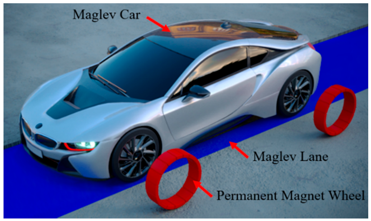
The PMEDS car system consists of a maglev car and maglev lane, as shown in Figure 1. The entire body of a maglev car is similar to a traditional car, except that the rubber wheel is embedded with the ring-shaped permanent magnet wheel. A non-ferromagnetic conductor plate is paved on the surface of ordinary roads as a special maglev lane. The PMEDS car can get rid of the constraints of the track existing in other classical maglev systems, and steer actively rather than being passively guided by the track. At the same time, the flat and simple maglev lane structure can be more easily integrated into the existing traffic infrastructure. In addition, the PMEDS car has strong adaptability, and can switch freely between a maglev car and conventional electric car. When the speed is low, a maglev car can run on ordinary roads, which is no different from a traditional car. When the maglev car needs to run at high speed, it can switch to the maglev lane and enter suspension mode, so as to reduce the resistance and greatly improve the driving speed. Therefore, it is expected to be a promising transportation tool in the future.

Our group designed and built a 1:50 PMEDS car model. Figure 2 shows its structure diagram and Figure 3 shows the experimental prototype of the PMEDS car. A maglev car is composed of four permanent magnet electrodynamic wheels (EDW), four brushless outer rotor DC motors, a chassis, and four auxiliary wheels. The permanent magnet EDW adopts the annular Halbach structure. The motors use a brushless outer rotor DC motor. The controller controls four motors separately.

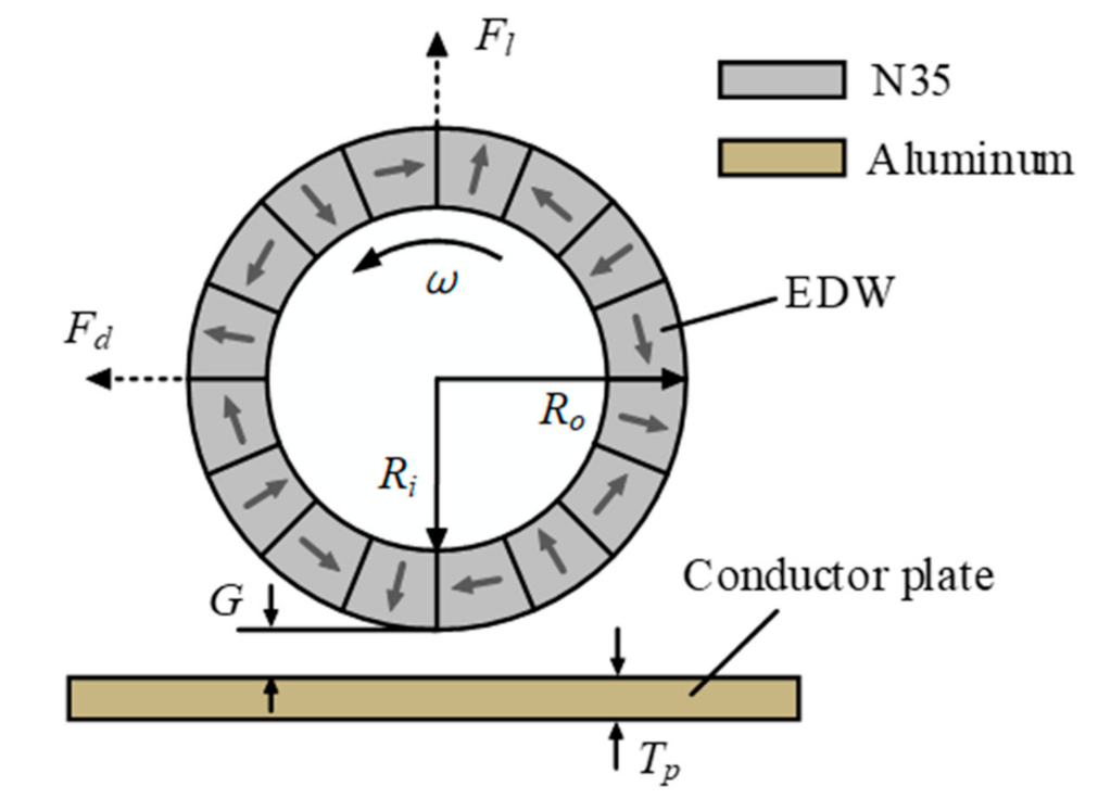
Magnetic wheels are the core components of a maglev car, and they are the direct source of levitation force and driving force. Figure 4 shows the structure and operating state of a permanent magnet EDW. The magnetic wheel adopts a four-pole annular Halbach structure, including 16 magnetic monomers. The permanent magnet array adopts radial and tangential magnetization methods to form the Halbach permanent magnet array, which has a strong magnetic field outside and a weak magnetic field inside.

The Halbach array is fixed on a horizontally placed outer rotor of the motor that rotates at high speed, which forms a time-varying magnetic field on the surface of the secondary induction plate that is located below the permanent magnet array. According to Lenz’s law, eddy current will be generated in the secondary induction plate. The interaction between the eddy current field and the external magnetic field will generate a repulsive force related to the magnetic induction intensity of the external magnetic field and the relative speed of movement. The tangential force is expressed as a driving force in the horizontal direction and the normal force is expressed as a levitation force that overcome the self-weight of the EDW. It makes full use of the characteristics of the annular Halbach structure permanent magnet array and converts the inherent magnetic resistance into the driving force in the direction of travel by rotating.

At this time, the driving force and the levitation force have a strong coupling relationship. The only factor affecting them is the relational speed between the magnetic wheel and the induction plate. Under the action of the driving force, the magnetic wheel generates the traveling speed in the forward direction, which makes the relative rotational speed of the magnetic wheel with the induction plate decrease and the suspension capacity gradually reduce, so a single suspension unit cannot achieve the integration of suspension and driving.

The rotational speed of four permanent magnet EDWs are controlled by motors to realize the suspension function and operating state control function. Figure 5 shows the schematic diagram of a PMEDS car model. The front EDWs turn counterclockwise at the rotational speed of ω₁ and the direction of magnetic resistance F_d1 is backward, while the rear EDWs turn clockwise at the rotational speed of ω₂ and the direction of magnetic resistance F_d2 is forward. The suspension function is achieved by synchronizing the rotational speed of the front and rear EDWs and turning in opposite directions, which generates driving force of the same size and opposite directions that offsets each other. At the same time, the levitation force F_l1+F_l2 generated by the four EDWs overcomes the weight of the entire device to achieve in-situ suspension. Then, the difference in driving force between the front and rear EDWs formed by different rotational speed is used to form a forward propulsion when F_d1<F_d2 or backward braking force when F_d1>F_d2 to realize a propulsion and braking function. In addition, by adjusting the difference in rotational speed on the left and right sides, the device is driven by different propulsion forces on the left and right sides and achieves a steering function.

3. Simplified Model of Electromagnetic Force

To provide electromagnetic force input for dynamic simulation to accurately analyze the dynamic response of the PMEDS system, it is necessary to transform the interaction relationship between the EDW and the conductor plate and establish a simplified electromagnetic force model. The main core of the PMEDS electromagnetic model is an induction eddy current model composed of a moving permanent magnet and an induction plate. There are two main research methods: one is the analytical approach, and the other is the numerical approach (mainly the finite element method). The circular geometry of the EDW combined with the linear geometry of the lane makes the analytical approach a formidable problem and both 2D and 3D analytical calculations lack an accurate and universal analytical equation. On the other hand, the research on the linear Halbach structure accounts for the majority of the PMEDS based on the Halbach structure. The research on the annular Halbach structure is less extensive and the methods are mostly equivalent to the linear Halbach structure. The calculation results are quite different. Therefore, in this paper we used the finite element method to carry out numerical calculations of the force of the suspension system, and studied the law of the levitation force and driving force with the system parameters, so as to obtain a simple and effective electromagnetic force mathematical model of the suspension system. Finally, the mathematical model was used to quantitatively describe the levitation force and driving force, which provides an effective reference for the characteristic analysis of PMEDS systems. We used the finite element analysis software Maxwell to numerically analyze the electromagnetic force characteristics of the EDW and proposed a simplified mathematical model of electromagnetic force for dynamic calculations. The mathematical model has a simple expression form and is more suitable for engineering calculations.

The outer radius of EDW was fixed to 50 mm according to the size ratio of car model. In order to reduce the eddy current loss and increase the levitation force, other parameters of EDW were optimized by Maxwell 2D simulation. The values of model parameters are shown in

Table 1. The parameters in the Maxwell 3D simulation.

Parameter	Value
Pole pairs, P	4
Remanence of permanent, Br/T	1.42
Inner radius of EDW, Ri/mm	34
Outer radius of EDW, Ro/mm	50
Width of EDW, Ww/mm	35
Width of Conductor Plate, Wp/mm	100
Thickness of Conductor Plate, Tp/mm	10
Conductivity of Conductor Plate, σ/(S/m)	3.8 × 107
Rotational speed ω/rpm	0~6000
Air gap, G/mm	5~15

. In order to make the simulation result closer to the experimental data, a simplified three-dimensional finite element model of the permanent magnet EDW was established, as shown in Figure 6. The model includes five parts: EDW, conductor plate, motion domain Band, and solution region. Since the EDW is rotating, the motion domain Band uses a polygonal cylinder to wrap the EDW. The material of EDW is N35 whose remanence is 1.42 T and the magnetization direction is set according to the ring Halbach. The material of the conductor plate is set to aluminum, and the motion domain Band and solution region are set as a vacuum. The rotational speed is set to 0 to 6000 rpm, while the air gap is set to 5 to 15 mm and the length step is 1 mm.

The boundary condition is defined as the infinity boundary condition which is called Balloon Boundary. The introduction of this boundary condition is a very ideal processing method because it removes the necessity of drawing the solution domain in a way that is too large, thereby reducing the overhead of computing resources such as the memory and CPU.

The excitation source consists of two parts: the first is the main excitation magnetic field provided by the permanent magnet, which has been completed in the material setting, and the second is the eddy current effect of the conductor plate, which is set in the excitations.

Due to the regular size of the model, the mesh division adopts manual division. Since the EDW and the motion domain band need to calculate their motion properties, their meshes are refined. The conductor plate is a fixed part, so its mesh size can be slightly enlarged. The mesh of the solution region can be divided into the maximum size. The meshing diagram of the permanent magnet EDW model is shown in Figure 7. The total number of meshes is 217,659.

Figure 8 shows the distribution of magnetic flux density in the conductor plate when the rotational speed of EDW is 3000 rpm and the air gap is 10 mm. The direction of the induction magnetic field is opposite to the magnetic field of EDW. The induction magnetic field below the EDW is stronger, which affects the levitation force and driving force. The maximum magnetic flux density can reach 0.4931 T.

Figure 9 shows the distribution of eddy current in the conductor plate when the rotational speed of EDW is 3000 rpm and the air gap is 10 mm. The eddy current is mainly concentrated in the rearward position below the wheel, and there are two current loops.

Figure 10 shows the levitation force and driving force of the EDW with different rotational speeds under different suspension air gaps. As shown in Figure 10a, the levitation force firstly increases rapidly with the increase of the rotation speed of the EDW and starts to increase slowly around 2000 rpm. This is because the higher the rotational speed of the EDW is, the greater the magnetic density passing through the conductor plate per unit time, which is equivalent to a faster frequency of the time-varying electromagnetic field, which induces a larger eddy current magnetic field in the induction plate so that the levitation force becomes greater. The levitation force tends to be stable at higher rotational speeds due to the saturation of the eddy current magnetic field. As shown in Figure 10b, the driving force firstly increases rapidly with the increase of the rotation speed of the EDW, reaching a peak at about 1200 rpm, and continues to decrease thereafter. This is because when the EDW runs at a low speed, the ampere force is related to the speed of the magnetic induction wire cutting induction plate, so the driving force is positively related to the speed. When the EDW runs at a high speed, the induced current is concentrated on the surface of the induction plate, and the vertical magnetic field related to the driving force is weakened, so the driving force is negatively related to the speed. Considering the actual application requirements, the finite element simulation model only calculates up to 6000 rpm. Under ideal conditions, as the speed increases indefinitely, the levitation force tends to stabilize, and the driving force attenuates close to zero. This phenomenon verifies the conclusion that PMEDS is suitable for high-speed and ultra-high-speed application scenarios.

For the EDW, the total power, P_total, includes the rotational power of EDW, P_EDW, for levitation and driving and the loss power, P_loss, in the form of heat in the conductor plate [27]. The P_EDW is computed from:

$$P_{EDW}=\frac{T\times n}{9550}=\frac{F_T\times R_o\times n}{9550}$$

(1)

where T is the torque computed by multiplying the load force by the outer radius, F_T is the load force, R_o is the outer radius, and n is the rotational speed. The P_loss in the conductor plate is obtained by Maxwell simulation. The EDW efficiency, η_EDW, is given by:

$${\eta }_{EDW}=\frac{P_{EDW}}{P_{total}}=\frac{P_{EDW}}{P_{EDW}+P_{loss}}$$

(2)

This ratio indicates the proportion of power that is used to create the levitation and driving forces.

The rotational speed of EDW has a significant effect on the performance. When the air gap is 10 mm, the power requirements with different rotational speed are shown in Figure 11. Figure 12 shows that the EDW efficiency increases with the increasing rotational speed. This is because at higher rotational speeds, the electrical frequency becomes higher and the induced eddy current in the conductor plate saturates gradually, which causes the loss power to stop increasing. The result is that the EDW power increases with an increasing rotational speed compared with the loss power and the EDW efficiency increases. The EDW efficiency is higher than 80% when the rotational speed is higher than 4500 rpm.

The establishment of a mathematical model requires determining the correlation coefficient according to the data fitting, and then obtaining the final mathematical fitting formula. The utilization of the MATLAB fitting toolbox for data fitting has the characteristics of a convenient solution and high accuracy. Therefore, the MATLAB fitting toolbox was selected as the surface fitting tool, and the best fitting formula was selected according to the goodness of fit test result that is the final mathematical model of the suspension characteristic curve.

In this article, the polynomial fitting of Matlab’s curve fitting toolbox cftool was selected as the method of data fitting. With the parameters of the suspension system fixed, the levitation force and driving force could be regarded as a binary function of the rotational speed of the EDW and the suspension air gap. We assumed that its functional form is:

$$F={\displaystyle \sum }_{i=0}^{n_1}{\displaystyle \sum }_{j=0}^{n_2}{p}_{ij}{x}^i{y}^j$$

(3)

where x is the rotational speed of the EDW, y is the suspension air gap, F is the electromagnetic force, p_ij is the polynomial coefficient, n₁ is the highest order of the rotational speed of the EDW, and n₂ is the highest order of the suspension air gap.

When using the fitting algorithm, the appropriate highest power should be selected, but a higher power is not better. This is because the Runge phenomenon is prone to occur when the power is too high, which results in large deviations in data point that outside the test point. The best fitting coefficients of the suspension characteristics are obtained by polynomial fitting. Finally, the mathematical models of the levitation force F_l and driving force F_d are:

$$\begin{array}{ll}{F}_l=& 0.13x-\left(2.23\times {10}^{-5}\right)x^2-0.02xy+\left(1.39\times {10}^{-9}\right)x^3\\ & +\left(2.78\times {10}^{-6}\right)x^{2}y+\left(1.35\times {10}^{-3}\right)x{y}^2-\left(1.43\times {10}^{-10}\right)x^{3}y\\ & -\left(1.28\times {10}^{-7}\right)x^2{y}^2-\left(4.65\times {10}^{-5}\right)x{y}^3\\ & +\left(4.01\times {10}^{-12}\right)x^3{y}^2+\left(2.12\times {10}^{-9}\right)x^2{y}^3\\ & +\left(6.63\times {10}^{-7}\right)x{y}^4\end{array}$$

(4)

$$\begin{array}{ll}{F}_d=& 0.13x-\left(6.14\times {10}^{-5}\right)x^2-0.02xy+\left(1.16\times {10}^{-8}\right)x^3\\ & +\left(5.90\times {10}^{-6}\right)x^{2}y+\left(8.48\times {10}^{-4}\right)x{y}^2-\left(9.44\times {10}^{-13}\right)x^4\\ & -\left(7.67\times {10}^{-10}\right)x^{3}y-\left(2.00\times {10}^{-7}\right)x^2{y}^2\\ & -\left(1.97\times {10}^{-5}\right)x{y}^3+\left(2.31\times {10}^{17}\right)x^5+\left(3.63\times {10}^{-14}\right)x^{4}y\\ & +\left(1.17\times {10}^{-11}\right)x^3{y}^2+\left(2.52\times {10}^{-9}\right)x^2{y}^3\\ & +\left(1.37\times {10}^{-7}\right)x{y}^4\end{array}$$

(5)

As the R-square of levitation force is 0.9896, and the R-square of driving force is 0.9874, the fitting degree is high. Therefore, the fitting model can be used as the electromagnetic force simplified mathematical model of EDW in the following dynamic simulation.

4. Operating Mode

The Adams is used to simulate the suspension performance and observe the changes in suspension air gap, levitation force, driving force, and translation speed in real time. The virtual prototype simulation software Adams developed by MSC in the United States, which is Automate Dynamic Analysis of Mechanical Systems, was developed based on the Lagrangian equation method of multi-body system dynamics and integrates system modeling, solving, and visualization technologies. Users can use Adams to perform statics, kinematics, and dynamics simulation analysis and it can be used to test the performance, peak load, and motion range of the mechanical system and calculation of the finite element input load. At the same time, its open program structure and multiple external interfaces can provide a secondary development research platform to analyze special types. It has always been favored by major automobile companies and researchers, and has been widely used in the automotive industry.

The use of Adams to solve dynamic problems mainly includes two steps: modeling and solving. Modeling is completed manually or imported by other software. In order to make the virtual prototype and the real object have a high degree of similarity, special solid modeling software Solidworks is used to model, assemble each part, and finally import. The total weight of PMEDS car model is 9.2 kg. During dynamic simulation with Adams, it is necessary to arrange the position coordinates of each component in the space, restrict the movement of each component by applying constraints, and import the simplified electromagnetic force model of the levitation force and driving force. It is also possible to add rotational speed function to left front (LF), right front (RF), left rear (LR), and right rear (RR) wheels separately. The three degree of freedom dynamic model of the PMEDS car is shown in Figure 13. Solving is completed through the software’s own solver. We analyzed the operating mode under three typical working conditions of static suspension, acceleration, and uniform speed, as well as deceleration and braking.

4.1. Static Suspension

When the PMEDS car is at static suspension, the front and rear EDWs rotate at the same speed in different directions. By gradually adjusting the speed of EDWs from 0 to 4000 rpm, the process shift of the PMEDS car from a stationary state on the ground to static suspension is simulated. The relationship between the suspension air gap and rotational speed of EDWs is shown in Figure 14.

From Figure 15, it can be known that the levitation force and driving force of the EDWs gradually increases with the increase of rotational speed before suspension. After the rotational speed of EDWs reaches 600 rpm (after 3 s), the levitation force of the EDWs is sufficient to balance the deadweight of the PMEDS car and achieve suspension. As the rotational speed of EDWs continues to increase, the levitation force needs to balance with the gravity, at which time it remains at about 23 N and no longer increases, which causes the suspension air gap to increase. Due to the fact that the damping of PMEDS is almost zero, the levitation force and the suspension air gap fluctuates and cannot be stabilized, and the maximum suspension air gap reaches 7.3 mm. The driving force gradually decreases and is stable at around 4 N under the combined effect of the increasing of the rotational speed of the EDWs and the suspension air gap. Stable suspension is achieved when the rotational speed of the EDWs reaches 3500 rpm. As shown in Figure 14, when the rotational speed of the EDWs is around 3500 rpm, the maglev car reaches the maximum suspension air gap and suspends stably. At the same time, as shown in Figure 15b, when the rotational speed is more than 3500 rpm, the driving force decreases gradually. In order to produce a larger driving force and improve the driving efficiency of a maglev car, the working rotational speed of EDWs was set as 3500 rpm.

4.2. Acceleration and Uniform Speed

The method adopted for acceleration is decelerating the rotational speed of the rear EDWs and keeping the rotational speed of the front EDWs constant, so that the forward driving force is greater than the backward driving force, which generates forward propulsion force to drive the PMEDS car to accelerate. From 1 s to 8 s, the rotational speed of all EDWs increases from 0 to 3500 rpm. The PMEDS car moves from a standstill state to static suspension. From 9 s to 10 s, the rotational speed of the rear EDWs decreases from 3500 rpm to 3000 rpm, and the PMEDS car begins to accelerate. From 10 s to 13 s, due to the existence of the car’s translation speed, the rotational speed of the front EDWs relative to the induction plate increases and the driving force decreases, while the rotational speed of the rear EDWs relative to the induction plate decreases and the driving force increases. In other words, the difference between the driving force of the front EDWs and rear EDWs becomes larger and larger. In this way, the propulsion force and the car’s translation speed will continue to increase, which makes the rotational speed of the rear EDWs relative to the induction plate decrease, and eventually results in a reduction in the levitation force and the loss of suspension capacity. Therefore, the rotational speed of the EDWs needs to be adjusted twice, so that the rotational speed of the front EDWs and rear EDWs relative to the induction plate are equal, the driving force offsets each other again, and the PMEDS car enters a uniform speed driving state. From 13 s to 14 s, the rotational speed of the rear EDWs increases from 3000 rpm to 4000 rpm and the translation speed of the PMEDS car stabilizes at 1.1 m/s. The entire acceleration process lasted 5 s and the average acceleration of PMEDS car is 0.22 m/s². The rotational speed regulation process of the EDWs during acceleration and uniform speed is shown in Figure 16. The relative rotational speed of the EDWs and the translation speed of the PMEDS car are respectively shown in Figure 17 and Figure 18.

4.3. Deceleration and Braking

The method commonly adopted for deceleration is to accelerate the rotational speed of rear EDWs, and the front EDWs are kept at a constant rotational speed, so that the forward driving force is smaller than the backward driving force, which generates a backward braking force to drive the PMEDS car to decelerate. The simulation process of the first 17 s is the same as the process of acceleration and uniform speed. Then in the case of constant translation speed, from 17 s to 18 s, the rotational speed of the rear EDWs increases from 4000 rpm to 4500 rpm, and the PMEDS car begins to decelerate. From 18 s to 22.5 s, the translation speed of the PMEDS car gradually decreases to zero. Similarly, the rotational speed of the EDWs is adjusted twice. From 22.5 s to 23.5 s, the rotational speed of the rear EDWs decreases from 4500 rpm to 3500 rpm. The relative rotational speed of the front and rear EDWs are synchronized again. The driving force offsets each other again. The PMEDS car is at static suspension, thus enabling the braking function. The entire deceleration process lasts 6.5 s and the average acceleration of the PMEDS car is 0.17 m/s². The rotational speed regulation process of the EDWs during acceleration, uniform speed, deceleration and braking is shown in Figure 19. The relative rotational speed of the EDWs and the translation speed of the PMEDS car are respectively shown in Figure 20 and Figure 21.

4.4. Efficiency

For the PMEDS car, there are two kinds of efficiency: EDW efficiency and PMEDS car efficiency. We evaluated the performance of PMEDS car from different perspectives.

The efficiency of EDW, η_EDW, indicates the efficiency of the EDW using motor power to rotate and is given by:

$${\eta }_{EDW}=\frac{P_{EDW}}{P_{EDW}+P_{loss}}=\frac{P_{EDW1}+P_{EDW2}}{P_{EDW1}+P_{EDW2}+P_{loss1}+P_{loss2}}$$

(6)

where the P_EDW is the rotational power of the four EDWs including the rotational power of the front wheels, P_EDW1, and the rotational power of the rear wheels, P_EDW2. The P_loss is the loss power of the four EDWs and includes the loss power of the front wheels, P_loss1, and the loss power of the rear wheels, P_loss2. While the P_EDW1 and P_EDW2 are computed by rotational speed as shown by (1), the P_loss1 and P_loss2 are computed by relative rotational speed of EDWs in a Maxwell simulation. When the PMEDS car runs at a constant speed, the P_loss1 is equal to the P_loss2 because the driving force is zero and the relative rotational speed are equal. The P_EDW1 is different from the P_EDW2 because under the influence of the translation speed, the front and rear EDWs rotate at different speed.

When the air gap is 10 mm, the EDW efficiency with different translation speeds is shown in Figure 22. When the translation speed is 0 m/s, the PMEDS car is at static suspension and the efficiency of EDW is 59.5%. As the translation speed increases, the EDW efficiency increases because of the increasing of the rotational speed. When the translation speed is 15 m/s, the EDW efficiency achieved is 82.9%.

The power of the car, P_car, indicates the efficiency of EDW to levitate and drive the car and is given by:

$$P_{car}=\left(F_{d2}-F_{d1}\right)V_x+\left(F_{l1}+F_{l2}\right)V_z$$

(7)

where the V_x is the horizontal speed and the V_z is the vertical speed of the PMEDS car. When the PMEDS car in the process of acceleration, the PMEDS car efficiency is shown in Figure 23. The variation of the horizontal speed is shown in Figure 18. When speed and air gap of the PMEDS are constant, the driving force calculated by F_d2 − F_d1 is zero and V_z is zero, so the power and the efficiency of the PMEDS car is always zero. From 8 s to 14 s, the horizontal speed increases from 0 to 1.1 m/s, while the efficiency of the PMEDS car increases because of the increasing of the horizontal speed and driving power and reaches the maximum value of 8.56% at 12.7 s. Due to getting rid of the ground friction and the neglecting of air resistance, the PMEDS car needs only a small amount of driving force to accelerate. Due to the small speed in the starting stage, the efficiency of PMEDS car is not high. When the PMEDS car runs at a higher speed, it has better efficiency and performance.

4.5. Feasibility of Real Size Car

The parameters used for the real size PMEDS car are given in

Table 2. The parameters of the real size PMEDS car.

Parameter	Value
Inner radius of EDW/mm	400
Outer radius of EDW/mm	260
Width of EDW/mm	280
Pole pairs of EDW	4
Wheelbase of car/mm	2920
Wheel-track of car/mm	1640
Mass of car/kg	2540

.

In order to directly reflect the force characteristics of the PMEDS car, a three-dimensional transient finite element model is established with Maxwell.

Figure 24 shows the levitation force and driving force of the real size EDW with different rotational speeds under different suspension air gaps. When the air gap is less than 40 mm and the rotational speed is greater than 500 rpm, an EDW can produce more than 10 kN levitation force. Four EDWs can produce more than 40 kN of levitation force and the PMEDS car achieves suspension and is manned. When the air gap is 40 mm, the maximum driving force is 3.7 kN.

5. Conclusions

We presented a new concept maglev car employing PMEDS which achieve the integration of suspension and driving. It applies maglev technology into the automotive field to design a new type of car, which provides constructive guidance for the development of ground transportation. The mathematical model of levitation force and driving force were established through data fitting combined with the finite element method, and the dynamic model of PMEDS car was established in Adams. Based on the dynamics model, the operating mode of the PMEDS car under static suspension, acceleration and uniform speed, deceleration and braking ware analyzed. The results show that the critical speed of the EDWs for suspension is 600 rpm, and the maximum suspension air gap for stable suspension can reach 7.3 mm. The working rotational speed of EDWs is 3500 rpm. At the same time, the movement status of the PMEDS car can be controlled by only adjusting the rotational speed of rear EDWs and in turn reducing the complexity of control system. The acceleration is related to the reduction of the rotational speed of rear EDWs. When the rear EDWs are reduced by 500 rpm, the PMEDS car can obtain 0.22 m/s² acceleration. Furthermore, this control method can accurately regulate the translation speed of a PMEDS car. After the 5 s acceleration process, the translation speed of the PMEDS car stabilizes at 1.1 m/s. The EDW and PMEDS cars are more efficient when they run at higher speeds. The levitation force of real size PMEDS car is more than 40 kN to achieve suspension while being manned. The functions of propulsion, acceleration, deceleration, and braking are realized and the feasibility of the PMEDS car system is verified by the experimental prototype. The simulation method has provided a valuable reference for the future design of the PMEDS car and a new maglev transportation system.