
Ecological–Economic Modelling of Traditional Agroforestry to Promote Farmland Biodiversity with Cost-Effective Payments

 , , and
Abstract
:1. Introduction
- What role do AES play in land use and sustaining orchard meadows?
- Which types of farms are more likely to implement AES and which measures?
- How does the cost effectiveness of AES differ between farm types?
- How would AES change the regional land use and affect the diversity of individual species?
2. Materials and Methods
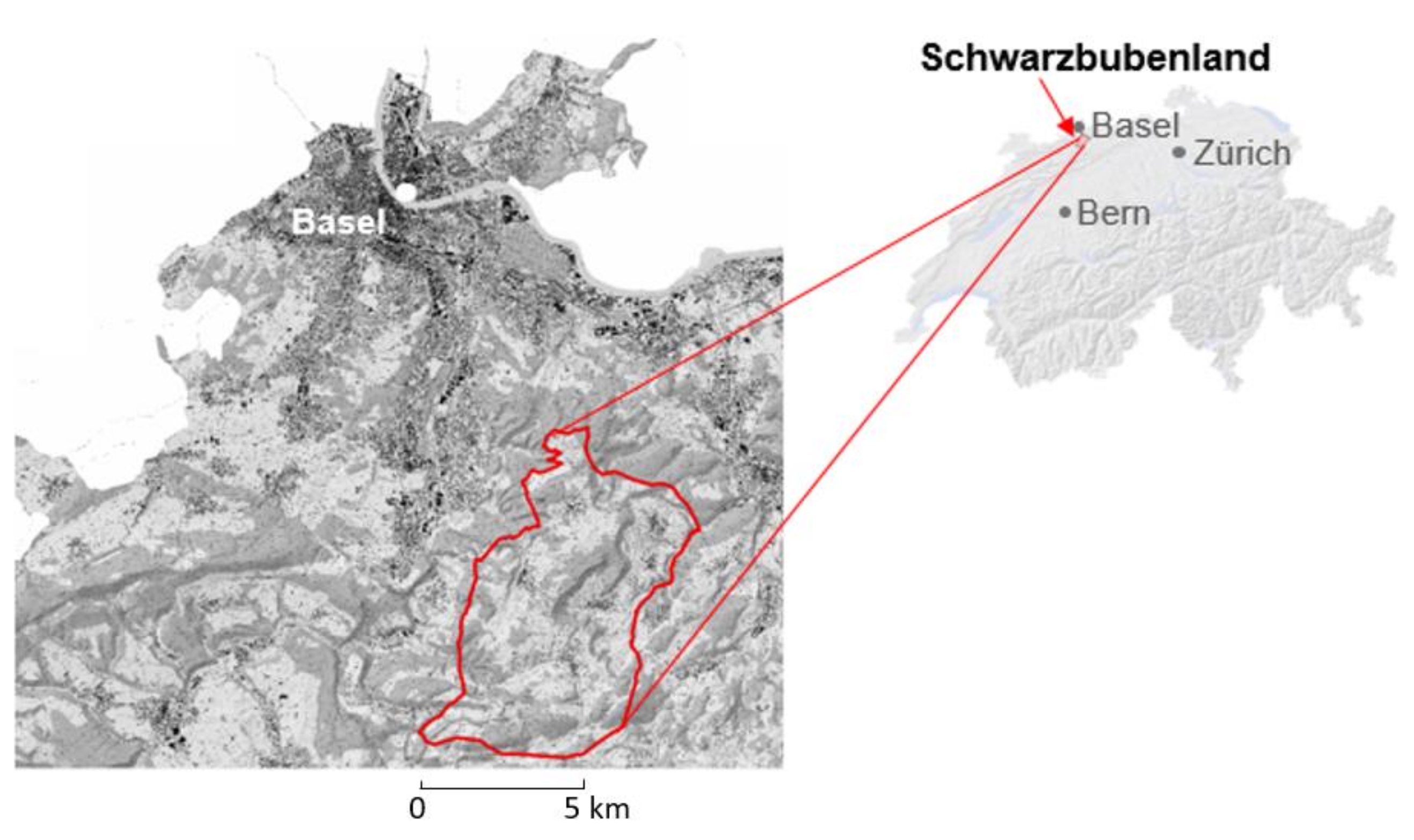
2.1. Case Study Region and Data
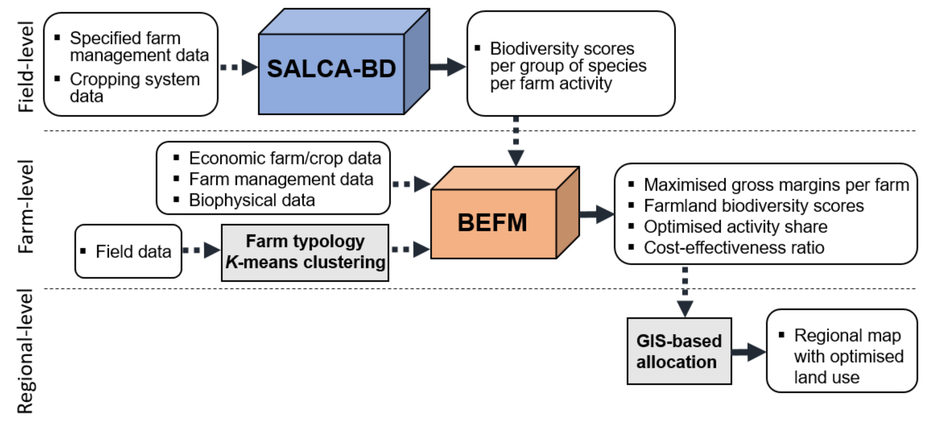
2.2. SALCA-BD (Swiss Agricultural Life Cycle Assessment—Biodiversity)
2.3. Farm Typology
2.4. BEFM (the Bio-Economic Farm Model)
2.4.1. General Approach
2.4.2. Farm Activities
2.4.3. Modules
2.4.4. Orchard Meadows
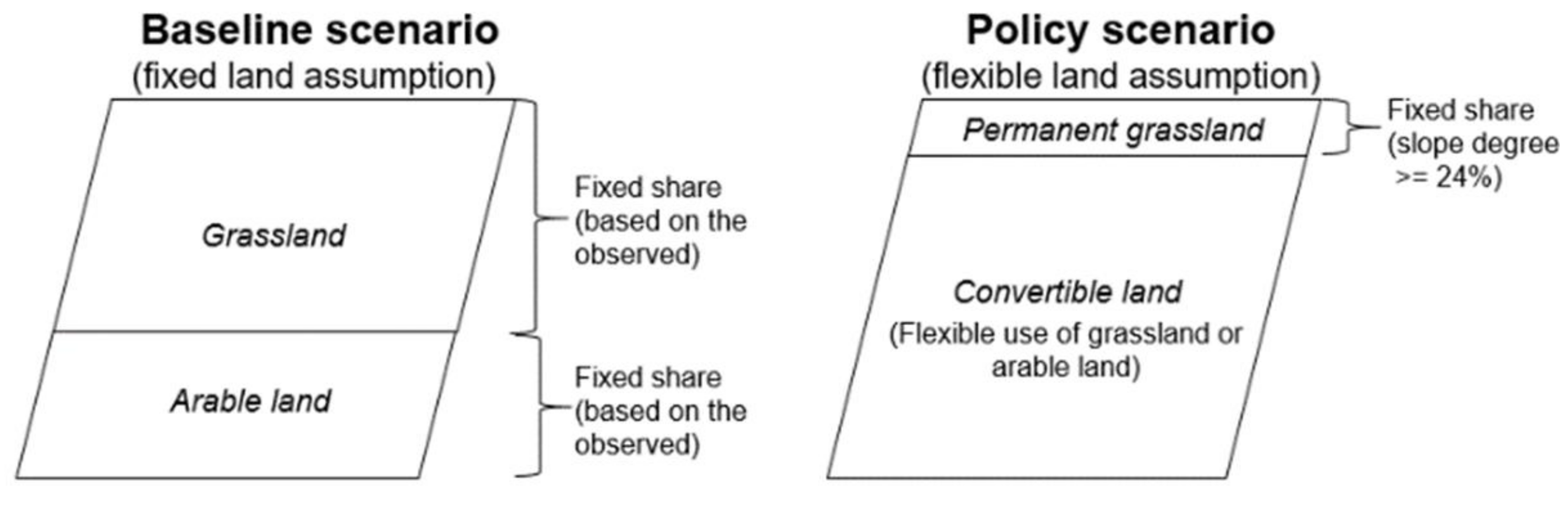
2.5. Policy Scenarios
2.6. Evaluation of Cost Effectiveness
2.7. Map Regional Change of Orchard Meadows
3. Results
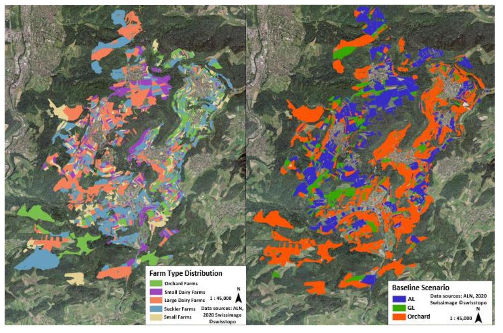
3.1. Farm Typology
3.2. Orchard Meadows with the Baseline Scenario
3.3. Policy Scenario
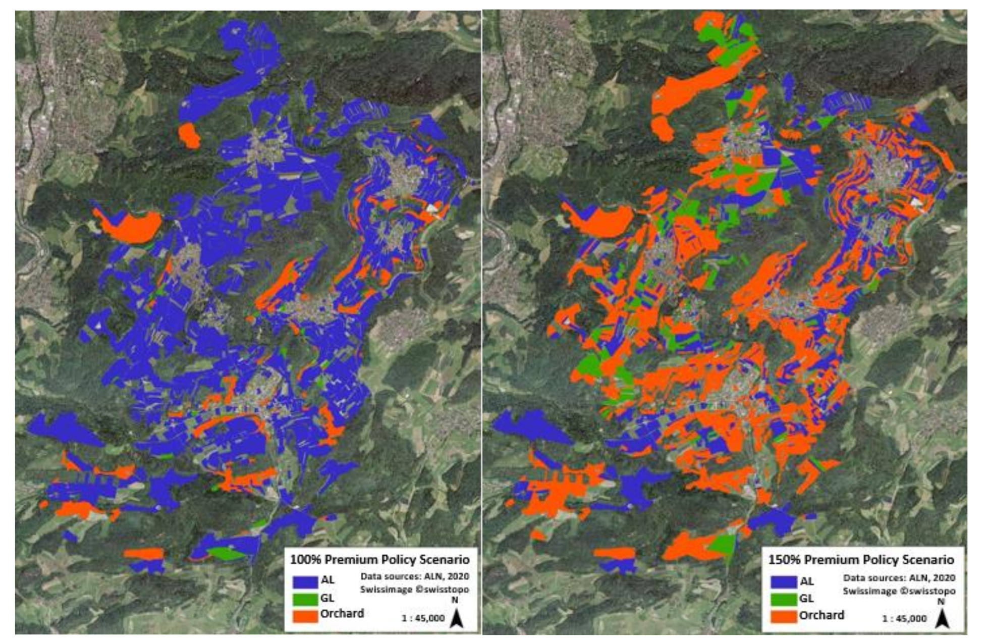
3.3.1. Role of AES in Land-Use and Sustaining Orchard Meadows
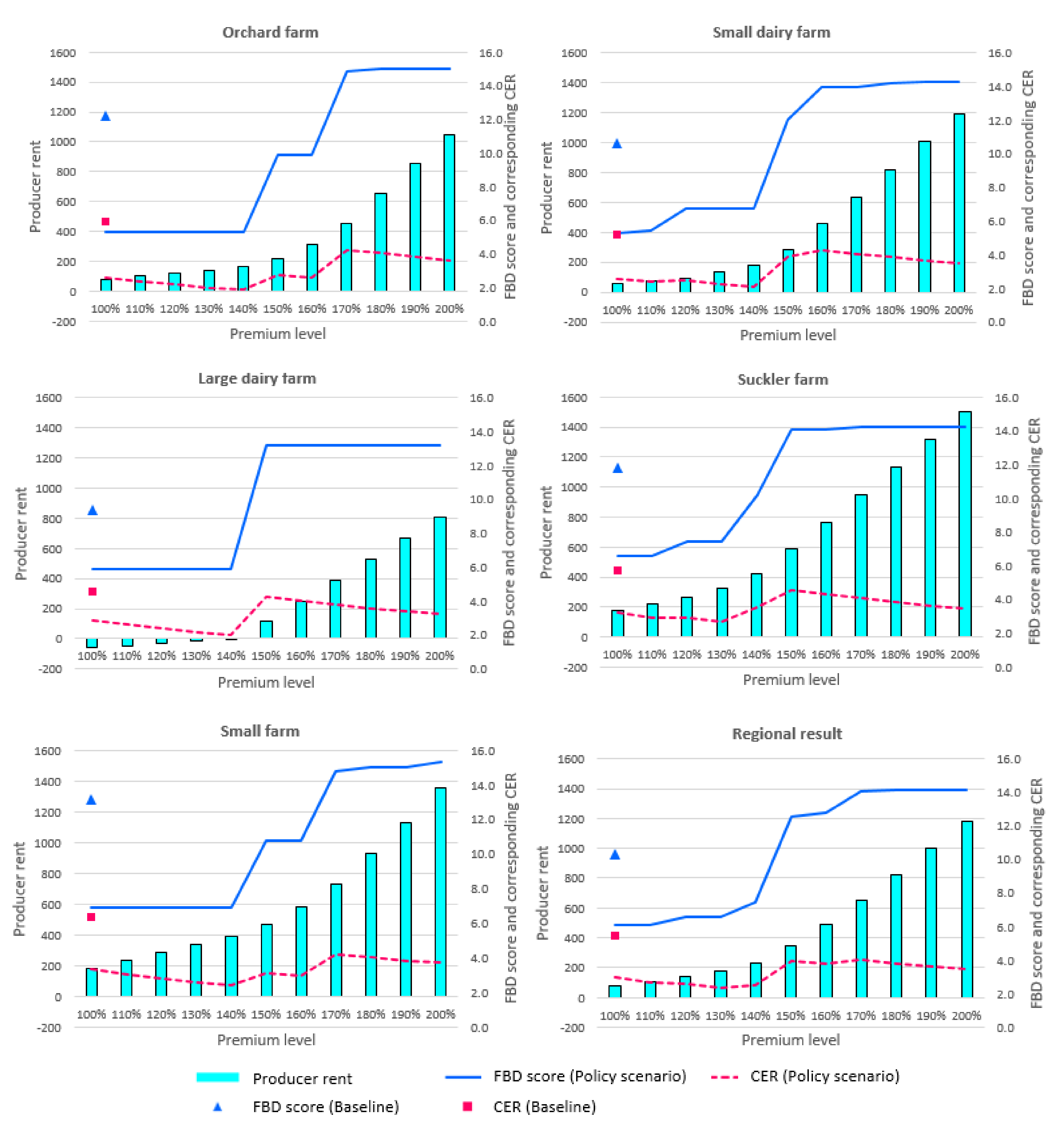
3.3.2. Difference in the Adoption of AES and the CER among Farm Types
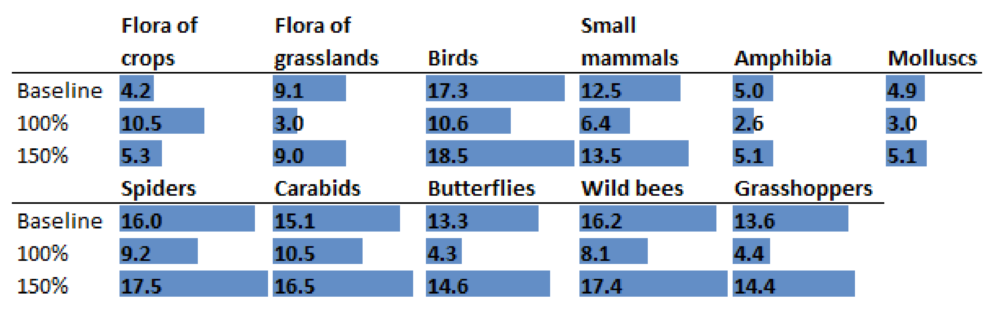
3.3.3. Change in the Regional Land Use and Individual Species Suitability with AES
4. Discussion
4.1. Orchard Meadows and Land-Use Change
4.2. Cost-Effectiveness and Its Difference over Farm Types
4.3. Methodological Limitations
4.4. Policy Implications
5. Conclusions
Supplementary Materials
Author Contributions
Funding
Institutional Review Board Statement
Informed Consent Statement
Data Availability Statement
Acknowledgments
Conflicts of Interest
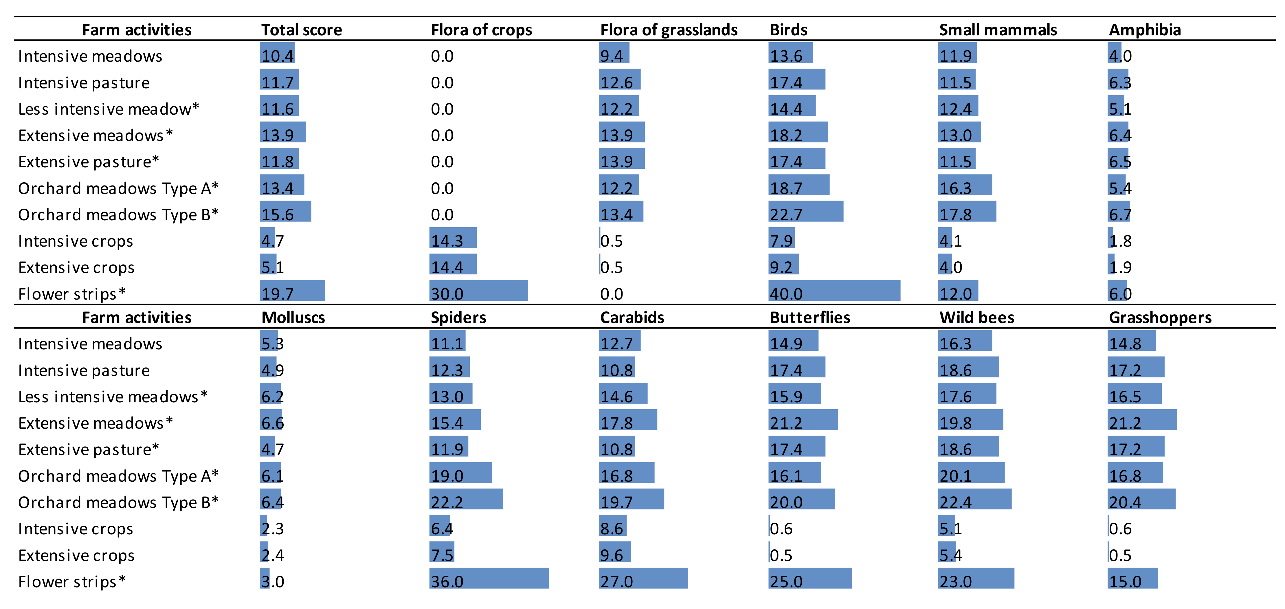
Appendix A. SALCA-BD Results
References
- BAFU. Biodiversität in der Schweiz: Zustand und Entwicklung; Bundesamt Für Umwelt: Bern, Switzerland, 2017. [Google Scholar]
- OECD. Reforming Agricultural Subsidies to Support Biodiversity in Switzerland; OECD: Paris, France, 2017. [Google Scholar]
- Bundesrat Verordnung Über Die Direktzahlungen an Die Landwirtschaft. Available online: https://www.fedlex.admin.ch/eli/cc/2013/765/de (accessed on 26 February 2022).
- OECD. Agricultural Policy Monitoring and Evaluation 2021: Addressing the Challenges Facing Food Systems; OECD: Paris, France, 2021. [Google Scholar] [CrossRef]
- Mack, G.; Ritzel, C.; Jan, P. Determinants for the implementation of action, result and multi-actor-oriented agri-environment schemes in Switzerland. Ecol. Econ. 2020, 176, 106715. [Google Scholar] [CrossRef]
- Herzog, F.; Jacot, K.; Tschumi, M.; Walter, T. The Role of Pest Management in Driving Agri-Environment Schemes in Switzerland. In Environmental Pest Management; John Wiley & Sons, Ltd.: Chichester, UK, 2017; pp. 385–403. [Google Scholar]
- Van Der Meer, M.; Kay, S.; Lüscher, G.; Jeanneret, P. What evidence exists on the impact of agricultural practices in fruit orchards on biodiversity? A systematic map. Environ. Evid. 2020, 9, 2. [Google Scholar] [CrossRef]
- Kay, S.; Crous-Duran, J.; García de Jalón, S.; Graves, A.; Palma, J.H.N.; Roces-Díaz, J.V.; Szerencsits, E.; Weibel, R.; Herzog, F. Landscape-scale modelling of agroforestry ecosystems services in Swiss orchards: A methodological approach. Landsc. Ecol. 2018, 33, 1633–1644. [Google Scholar] [CrossRef] [Green Version]
- Bailey, D.; Schmidt-Entling, M.H.; Eberhart, P.; Herrmann, J.D.; Hofer, G.; Kormann, U.; Herzog, F. Effects of habitat amount and isolation on biodiversity in fragmented traditional orchards. J. Appl. Ecol. 2010, 47, 1003–1013. [Google Scholar] [CrossRef]
- Plieninger, T.; Levers, C.; Mantel, M.; Costa, A.; Schaich, H.; Kuemmerle, T. Patterns and drivers of scattered tree loss in agricultural landscapes: Orchard meadows in Germany (1968–2009). PLoS ONE 2015, 10, e0126178. [Google Scholar] [CrossRef] [PubMed]
- Schönhart, M.; Schauppenlehner, T.; Schmid, E.; Muhar, A. Analysing the maintenance and establishment of orchard meadows at farm and landscape levels applying a spatially explicit integrated modelling approach. J. Environ. Plan. Manag. 2011, 54, 115–143. [Google Scholar] [CrossRef]
- Baroffio, C.A.; Richoz, P.; Fischer, S.; Kuske, S.; Linder, C.; Kehrli, P. Monitoring drosophila suzukii in Switzerland in 20121. J. Berry Res. 2014, 4, 47–52. [Google Scholar] [CrossRef] [Green Version]
- Knoll, V.; Ellenbroek, T.; Romeis, J.; Collatz, J. Seasonal and regional presence of hymenopteran parasitoids of drosophila in Switzerland and their ability to parasitize the invasive drosophila suzukii. Sci. Rep. 2017, 7, 40697. [Google Scholar] [CrossRef]
- ALW. Auswirkungen der AP 14 17 auf die Landwirtschaft im Kanton Solothurn; Amt für Landwirtschaft: Kanton Solothurn, Switzerland, 2019. [Google Scholar]
- Sereke, F.; Graves, A.R.; Dux, D.; Palma, J.H.N.; Herzog, F. Innovative agroecosystem goods and services: Key profitability drivers in Swiss agroforestry. Agron. Sustain. Dev. 2015, 35, 759–770. [Google Scholar] [CrossRef] [Green Version]
- Huber, R.; Zabel, A.; Schleiffer, M.; Vroege, W.; Brändle, J.M.; Finger, R. Conservation costs drive enrolment in agglomeration bonus scheme. Ecol. Econ. 2021, 186, 107064. [Google Scholar] [CrossRef]
- Hanley, N.; Acs, S.; Dallimer, M.; Gaston, K.J.; Graves, A.; Morris, J.; Armsworth, P.R. Farm-scale ecological and economic impacts of agricultural change in the uplands. Land Use Policy 2012, 29, 587–597. [Google Scholar] [CrossRef]
- Armsworth, P.R.; Acs, S.; Dallimer, M.; Gaston, K.J.; Hanley, N.; Wilson, P. The cost of policy simplification in conservation incentive programs. Ecol. Lett. 2012, 15, 406–414. [Google Scholar] [CrossRef] [PubMed]
- Bamière, L.; Havlík, P.; Jacquet, F.; Lherm, M.; Millet, G.; Bretagnolle, V. Farming system modelling for agri-environmental policy design: The case of a spatially non-aggregated allocation of conservation measures. Ecol. Econ. 2011, 70, 891–899. [Google Scholar] [CrossRef]
- Wunder, S.; Brouwer, R.; Engel, S.; Ezzine-De-Blas, D.; Muradian, R.; Pascual, U.; Pinto, R. From principles to practice in paying for nature’s services. Nat. Sustain. 2018, 1, 145–150. [Google Scholar] [CrossRef]
- Ansell, D.; Freudenberger, D.; Munro, N.; Gibbons, P. The cost-effectiveness of agri-environment schemes for biodiversity conservation: A quantitative review. Agric. Ecosyst. Environ. 2016, 225, 184–191. [Google Scholar] [CrossRef]
- Wuepper, D.; Huber, R. Comparing effectiveness and return on investment of action and results-based agri-environmental payments in Switzerland. Am. J. Agric. Econ. 2021. [Google Scholar] [CrossRef]
- Wunder, S.; Brouwer, R.; Engel, S.; Ezzine-de-Blas, D.; Muradian, R.; Pascual, U.; Pinto, R. Reply to: In defence of simplified PES designs. Nat. Sustain. 2020, 3, 428–429. [Google Scholar] [CrossRef]
- ALW. Agrarinformationen Kanton Solothurn—Tierhaltung, Flächennutzung, Ressourceneffizienz, BFF, LQB; Amt für Landwirtschaft: Kanton Solothurn, Switzerland, 2020. [Google Scholar]
- FSO. Farm Structure Survey. Federal Statistical Office. Available online: https://www.bfs.admin.ch/bfs/en/home/statistics/agriculture-forestry/farming.html/ (accessed on 26 February 2022).
- Jeanneret, P.; Baumgartner, D.U.; Freiermuth Knuchel, R.; Koch, B.; Gaillard, G. An expert system for integrating biodiversity into agricultural life-cycle assessment. Ecol. Indic. 2014, 46, 224–231. [Google Scholar] [CrossRef]
- Lüscher, G.; Nemecek, T.; Arndorfer, M.; Balázs, K.; Dennis, P.; Fjellstad, W.; Friedel, J.K.; Gaillard, G.; Herzog, F.; Sarthou, J.P.; et al. Biodiversity assessment in LCA: A validation at field and farm scale in eight European regions. Int. J. Life Cycle Assess. 2017, 22, 1483–1492. [Google Scholar] [CrossRef] [Green Version]
- Bholowalia, P.; Kumar, A. EBK-means: A clustering technique based on elbow method and k-means in WSN. Int. J. Comput. Appl. 2014, 105, 975–8887. [Google Scholar]
- Andersen, E.; Elbersen, B.; Godeschalk, F.; Verhoog, D. Farm management indicators and farm typologies as a basis for assessments in a changing policy environment. J. Environ. Manag. 2007, 82, 353–362. [Google Scholar] [CrossRef] [PubMed]
- Schuler, J.; Toorop, R.A.; Willaume, M.; Vermue, A.; Schläfke, N.; Uthes, S.; Zander, P.; Rossing, W. Assessing climate change impacts and adaptation options for farm performance using bio-economic models in Southwestern France. Sustainability 2020, 12, 7528. [Google Scholar] [CrossRef]
- Uthes, S.; Piorr, A.; Zander, P.; Bieńkowski, J.; Ungaro, F.; Dalgaard, T.; Stolze, M.; Moschitz, H.; Schader, C.; Happe, K.; et al. Regional impacts of abolishing direct payments: An integrated analysis in four European regions. Agric. Syst. 2011, 104, 110–121. [Google Scholar] [CrossRef]
- Kaiser, H.M.; Messer, K.D. Mathematical Programming for Agricultural, Environmental, and Resource Economics; Wiley: Hoboken, NJ, USA, 2011; ISBN 9780470599365. [Google Scholar]
- Mason, A.J. OpenSolver—An Open Source Add-in to Solve Linear and Integer Programmes in Excel; Springer: Berlin/Heidelberg, Germany, 2012; pp. 401–406. [Google Scholar] [CrossRef]
- Böcker, T.; Möhring, N.; Finger, R. Herbicide free agriculture? A bio-economic modelling application to Swiss wheat production. Agric. Syst. 2019, 173, 378–392. [Google Scholar] [CrossRef]
- Agristat, 2003-2020. In Statistische Erhebungen und Schätzungen über Landwirtschaft und Ernährung (SES); Schweizer Bauernverband: Brugg, Switzerland, 2021.
- AGRIDEA (Swiss Association for the Development of Agriculture and Rural Areas). Deckungsbeiträge DBKAT; AGRIDEA: Lausanne, Switzerland, 2020. [Google Scholar]
- Agroscope. 8/Düngung von Ackerkulturen: Grundlagen für Die Düngung Landwirtschaftlicher Kulturen in der Schweiz. In Grundlagen für die Düngung Landwirtschaftlicher Kulturen in der Schweiz (GRUD); Agroscope: Bern, Switzerland, 2017. [Google Scholar]
- Reidsma, P.; Janssen, S.; Jansen, J.; van Ittersum, M.K. On the development and use of farm models for policy impact assessment in the European union—A review. Agric. Syst. 2018, 159, 111–125. [Google Scholar] [CrossRef]
- Janssen, S.; Louhichi, K.; Kanellopoulos, A.; Zander, P.; Flichman, G.; Hengsdijk, H.; Meuter, E.; Andersen, E.; Belhouchette, H.; Blanco, M.; et al. A generic bio-economic farm model for environmental and economic assessment of agricultural systems. Environ. Manag. 2010, 46, 862–877. [Google Scholar] [CrossRef] [Green Version]
- FEEDBASE (The Swiss Feed Database). Available online: https://www.feedbase.ch/ (accessed on 20 February 2022).
- DLG-Akademie. DLG Futterwerttabellen Wiederkäuer; DLG-Verlag Frankfurt: Hessen, Germany, 1997. [Google Scholar]
- Giannitsopoulos, M.L.; Graves, A.R.; Burgess, P.J.; Crous-Duran, J.; Moreno, G.; Herzog, F.; Palma, J.H.N.; Kay, S.; García de Jalón, S. Whole system valuation of arable, agroforestry and tree-only systems at three case study sites in Europe. J. Clean. Prod. 2020, 269, 122283. [Google Scholar] [CrossRef]
- Schönhart, M.; Schauppenlehner, T.; Schmid, E. Integrated Bio-Economic Farm Modeling for Biodiversity Assessment at Landscape Level. In Bio-Economic Models Applied to Agricultural Systems; Flichman, G., Ed.; Springer: Dordrecht, The Netherlands, 2011; ISBN 978-94-007-1902-6. [Google Scholar]
- Drechsler, M. Ecological-Economic Modelling for Biodiversity Conservation; Cambridge University Press: Cambridge, UK, 2020. [Google Scholar] [CrossRef]
- Schweizer Bauernverband Preise Pflanzenbau. Available online: https://www.sbv-usp.ch/de/preise/pflanzenbau/ (accessed on 22 May 2021).
- Bundesrat Verordnung Über Einzelkulturbeiträge Im Pflanzenbau Und Die Zulage Für Getreide. Available online: https://www.fedlex.admin.ch/eli/cc/2013/873/de (accessed on 26 February 2022).
- Bethwell, C.; Burkhard, B.; Daedlow, K.; Sattler, C.; Reckling, M.; Zander, P. Towards an enhanced indication of provisioning ecosystem services in agro-ecosystems. Environ. Monit. Assess. 2021, 193, 269. [Google Scholar] [CrossRef]
- Wrbka, T.; Erb, K.H.; Schulz, N.B.; Peterseil, J.; Hahn, C.; Haberl, H. Linking pattern and process in cultural landscapes. An empirical study based on spatially explicit indicators. Land Use Policy 2004, 21, 289–306. [Google Scholar] [CrossRef]
- Wang, X.; Dietrich, J.P.; Lotze-Campen, H.; Biewald, A.; Stevanović, M.; Bodirsky, B.L.; Brümmer, B.; Popp, A. Beyond land-use intensity: Assessing future global crop productivity growth under different socioeconomic pathways. Technol. Forecast. Soc. Chang. 2020, 160, 120208. [Google Scholar] [CrossRef]
- Uthes, S.; Matzdorf, B. Studies on agri-environmental measures: A survey of the literature. Environ. Manag. 2012, 51, 251–266. [Google Scholar] [CrossRef] [PubMed]
- Kuhfuss, L.; Begg, G.; Flanigan, S.; Hawes, C.; Piras, S. Should Agri-Environmental Schemes Aim at Coordinating Farmers’ Pro-Environmental Practices? A Review of the Literature. In Proceedings of the 172nd EAAE Seminar, Brussels, Belgium, 28–29 May 2019. [Google Scholar]
- Manning, P.; Van Der Plas, F.; Soliveres, S.; Allan, E.; Maestre, F.T.; Mace, G.; Whittingham, M.J.; Fischer, M. Redefining ecosystem multifunctionality. Nat. Ecol. Evol. 2018, 2, 427–436. [Google Scholar] [CrossRef]
- Fastré, C.; van Zeist, W.J.; Watson, J.E.M.; Visconti, P. Integrated spatial planning for biodiversity conservation and food production. One Earth 2021, 4, 1635–1644. [Google Scholar] [CrossRef]
- Chopin, P.; Bergkvist, G.; Hossard, L. Modelling biodiversity change in agricultural landscape scenarios—A review and prospects for future research. Biol. Conserv. 2019, 235, 1–17. [Google Scholar] [CrossRef]
- Mennig, P.; Sauer, J. The impact of agri-environment schemes on farm productivity: A DID-matching approach. Eur. Rev. Agric. Econ. 2020, 47, 1045–1093. [Google Scholar] [CrossRef]
- Overmars, K.P.; Helming, J.; van Zeijts, H.; Jansson, T.; Terluin, I. A modelling approach for the assessment of the effects of common agricultural policy measures on farmland biodiversity in the EU27. J. Environ. Manag. 2013, 126, 132–141. [Google Scholar] [CrossRef]
- Sinaga, K.P.; Yang, M.S. Unsupervised K-Means Clustering Algorithm. IEEE Access 2020, 8, 80716–80727. [Google Scholar] [CrossRef]


| Grassland (Fodder) | Arable Land (Fodder) | Arable Land (Cash Crops) | |||
|---|---|---|---|---|---|
| Intensive | Meadow | Intensive | Fodder wheat | Intensive | Spelt wheat |
| Pasture | Triticale | Winter Wheat | |||
| Less intensive | Meadow 1 | Oats | Spring wheat | ||
| Extensive | Meadow 1 | Winter barley | Rye | ||
| Pasture 1 | Ley pasture | Extensive | Spelt wheat | ||
| Orchard- | Extensive | Fodder wheat | Winter Wheat | ||
| Meadow 1 | Triticale | Spring wheat | |||
| Oats | Rye | ||||
| Livestock | Winter barley | Flower strips 1 | |||
| Dairy cow | Ley pasture | ||||
| Suckler cow | White peas | ||||
| Young stock | Silo-green corn | ||||
| Dairy Cow | Suckler Cow | |||
|---|---|---|---|---|
| Adult Cow | Youngstock | Adult Cow | Youngstock | |
| Maximum DM intake per day (kg) | 16.8 | 12.5 | 14.0 | 7.8 |
| Minimum NEL per day (MJ) | 105.0 | 47.1 | 80.0 | 36.1 |
| Minimum crude-protein per day (kg) | 2.3 | 1.2 | 1.9 | 0.9 |
| Minimum crude-fiber per day (kg) | 3.4 | 2.4 | 2.8 | 1.4 |
| Type of Restrictions | Explanation |
|---|---|
| Restrictions to qualify for direct payments | Crop rotation cereals (without corn and oats < 66% of AL), crop ration wheat, spelt and triticale (<50% of AL), crop rotation oats (<25% of AL), crop rotation corn (<40% of AL), crop rotation white peas (<15% of AL), flower strips (<50% of AL), biodiversity measure (>7% of total farmland), minimal livestock intensity, grassland-based milk and meat program 1 |
| Restrictions based on expert knowledge | Pasture limitation (less than 50% of grassland), nutritional balance (upper limit of DM intake, minimum NEL, crude protein and crude fiber), permanent GL (slope degree ≥ 24%), crop rotation limit cereals (<80% of AL) |
| Restrictions based on statistics | Total farm size, area of permanent GL, GL and AL, area of flexible land, labor hour, youngstock balance (share of offspring to adult cows), stable capacity |
| Biodiversity Measures (EFA) | Quality Measure I | Quality Measure II | Modeled Payment |
|---|---|---|---|
| Extensive meadow (CHF ha−1) | 860 | 1840 | 860 |
| Less intensive meadow (CHF ha−1) | 450 | 1200 | 450 |
| Extensive pasture (CHF ha−1) | 450 | 700 | 450 |
| High-stem fruit trees (CHF tree−1) | 13.5 | 31.5 | 39.8 |
| Orchard meadow Type A (CHF ha−1) (CHF/ha) | - | - | 1642 |
| Orchard meadow Type B (CHF/ha−1) | - | - | 2052 |
| Flower strips (CHF ha−1) | 2500 | - | 2500 |
| Orchard Meadow Type A | Orchard Meadow Type B | Source | |
|---|---|---|---|
| Description | Commercial cherry production | No cherry production (maintaining trees for AES) | |
| Trees | 30 trees ha−1 | 30 trees ha−1 | Own source |
| Cherry yield | 30 kg tree−1 | - | Giannitsopoulos 2020 |
| Cherry price | 1.5/1.2/0.7 CHF kg−1 | - | Giannitsopoulos 2020 |
| Meadow management | Less intensive (2 cuts year−1) | Extensive (1 cut year−1, no fertilizer) | |
| Forage yield loss | −15% less (yield: 54 dt ha−1) | −10% less (yield: 23 dt ha−1) | According to a local expert |
| Annual replanting | 0.5 tree ha−1 | 0.5 tree ha−1 | Schönhart 2011a |
| Establishment cost | 140 CHF tree−1 | 140 CHF tree−1 | Giannitsopoulos 2020 |
| Maintenance cost 2 | 6585 CHF ha−1 | 630 CHF ha−1 | Giannitsopoulos 2020 |
| Clearing cost 1 | 60 CHF tree−1 | 60 CHF tree−1 | Giannitsopoulos 2020 |
| Labor | 44 h ha−1 | 27 h ha−1 | Giannitsopoulos 2020 |
| Subsidy for trees | 39.8 CHF tree−1 | 39.8 CHF tree−1 | Bundesrat 2016 |
| Total subsidy | 2393 CHF ha−1 | 2803 CHF ha−1 | Bundesrat 2016 |
| Total revenues | 3743 CHF ha−1 (1.5 CHF kg−1) 3473 CHF ha−1 (1.2 CHF kg−1) 3050 CHF ha−1 (0.7 CHF kg−1) | 2803 CHF ha−1 | |
| Total costs 1 | 6837 CHF ha−1 | 882 CHF ha−1 | |
| GM with subsidy | −3094 CHF ha−1 (1.5 CHF/kg) −3364 CHF ha−1 (1.2 CHF/kg) −3787 CHF ha−1 (0.7 CHF/kg) | 1921 CHF ha−1 |
| Orchard | Small Dairy | Large Dairy | Suckler Farm | Small Farm | |
|---|---|---|---|---|---|
| Farm size (ha) | 34.8 | 19.9 | 40.7 | 33.6 | 8.5 |
| Weight for aggregation | 14% | 12% | 30% | 32% | 12% |
| Initial grassland share | 72% | 60% | 56% | 70% | 81% |
| Of which extensive grassland | 41% | 29% | 19% | 31% | 46% |
| Permanent grassland | 9.4% | 10.5% | 8.1% | 5.9% | 24.8% |
| Livestock | no | yes | yes | yes | No |
| Livestock intensity (LSU ha−1) | - | 0.6 | 1.1 | 0.8 | - |
| Capacity of livestock (LSU) | - | 12 | 43 | 26 | - |
| Labor availability in AWU | 0.5 | 1.34 | 1.9 | 1.34 | 0.2 |
| Grassland-based milk and meat program 1 | - | no | yes | yes | - |
| GM | Subsidy to GM | EFA (%) | Trees | FBD Score | CER | Producer-Rent | Grass Land | Orchard | Arable Land | |
|---|---|---|---|---|---|---|---|---|---|---|
| Orchard | 73,322 | 113% | 72% | 755 | 12.2 | 6.0 | 541 | 0% | 72% | 28% |
| Small dairy | 83,414 | 51% | 52% | 313 | 10.6 | 5.2 | 589 | 8% | 52% | 40% |
| Large dairy | 236,446 | 31% | 29% | 350 | 9.4 | 4.6 | 256 | 28% | 29% | 44% |
| Suckler farm | 101,440 | 77% | 65% | 659 | 11.8 | 5.8 | 702 | 5% | 65% | 30% |
| Small farm | 17,048 | 122% | 81% | 206 | 13.2 | 6.4 | 605 | 0% | 81% | 19% |
Publisher’s Note: MDPI stays neutral with regard to jurisdictional claims in published maps and institutional affiliations. |
© 2022 by the authors. Licensee MDPI, Basel, Switzerland. This article is an open access article distributed under the terms and conditions of the Creative Commons Attribution (CC BY) license (https://creativecommons.org/licenses/by/4.0/).
Share and Cite
Nishizawa, T.; Kay, S.; Schuler, J.; Klein, N.; Herzog, F.; Aurbacher, J.; Zander, P. Ecological–Economic Modelling of Traditional Agroforestry to Promote Farmland Biodiversity with Cost-Effective Payments. Sustainability 2022, 14, 5615. https://doi.org/10.3390/su14095615
Nishizawa T, Kay S, Schuler J, Klein N, Herzog F, Aurbacher J, Zander P. Ecological–Economic Modelling of Traditional Agroforestry to Promote Farmland Biodiversity with Cost-Effective Payments. Sustainability. 2022; 14(9):5615. https://doi.org/10.3390/su14095615
Chicago/Turabian StyleNishizawa, Takamasa, Sonja Kay, Johannes Schuler, Noëlle Klein, Felix Herzog, Joachim Aurbacher, and Peter Zander. 2022. "Ecological–Economic Modelling of Traditional Agroforestry to Promote Farmland Biodiversity with Cost-Effective Payments" Sustainability 14, no. 9: 5615. https://doi.org/10.3390/su14095615
APA StyleNishizawa, T., Kay, S., Schuler, J., Klein, N., Herzog, F., Aurbacher, J., & Zander, P. (2022). Ecological–Economic Modelling of Traditional Agroforestry to Promote Farmland Biodiversity with Cost-Effective Payments. Sustainability, 14(9), 5615. https://doi.org/10.3390/su14095615