Essay

Spatio-Temporal Dynamics and Driving Forces of Multi-Scale Emissions Based on Nighttime Light Data: A Case Study of the Pearl River Delta Urban Agglomeration

1
College of Mining Engineering, North China University of Science and Technology, Tangshan 063210, China
2
Tangshan Key Laboratory of Resources and Environmental Remote Sensing, Tangshan 063210, China
3
Hebei Industrial Technology Institute of Mine Ecological Remediation, Tangshan 063210, China
4
Hebei Key Laboratory of Mining Development and Security Technology, Tangshan 063210, China
5
No.2 Geological Brigade of Hebei Bureau of Geology and Mineral Resources Exploration, Tangshan 063210, China
*
Author to whom correspondence should be addressed.
Sustainability 2023, 15(10), 8234; https://doi.org/10.3390/su15108234
Submission received: 13 April 2023 / Revised: 16 May 2023 / Accepted: 17 May 2023 / Published: 18 May 2023
(This article belongs to the Section Energy Sustainability)

Abstract

:
It is of great significance to formulate differentiated carbon emission reduction policies to clarify spatio-temporal characteristics and driving factors of carbon emissions in different cities and cities at different scales. By fitting nighttime light data (NTL) of long time series from 2000 to 2020, a carbon emission estimation model of Pearl River Delta urban agglomeration at city, county, and grid unit levels was built to quickly and accurately estimate carbon emission in the Delta cities above county level. Combining spatial statistics, spatial autocorrelation, Emerging Spatio-Temporal Hotspot Analysis (ES-THA), and Theil index (TL), this study explored the spatio-temporal differentiation of urban carbon emissions in the Delta and used a geographical detector to determine the influencing factors of the differentiation. The results of the study showed that NTL could replace a statistical yearbook in calculating carbon emissions of cities at or above county level. The calculation error was less than 18.7385% in the Delta. The three levels of carbon emissions in the Delta increased in a fluctuating manner, and the spatial distribution difference in carbon emissions at the municipal and county levels was small. Therefore, a combination of municipal and county scales can be implemented to achieve precise emission reduction at both macro and micro levels. The central and eastern parts of the agglomeration, including Guangzhou (Gz), Shenzhen (Sz), Zhongshan (Zs), and Huizhou (Hz), were a high-value clustering and spatio-temporal hot spots of carbon emissions. Zhaoqing (Zq) in the northwestern part of the agglomeration has always been a low-value clustering and a spatio-temporal cold spot because of its population, economy, and geographical location. The carbon emission differences in the Delta cities were mainly caused by carbon emission differences within the cities at the municipal level, and the cities faced the challenge of regional differences in the reduction in per capita carbon emissions. As the most influential single factor, spatial interaction between economic development and various factors was the main driving force for the growth of carbon emissions. Therefore, the results of this study provide a scientific theory and information support for carbon emission estimation and prediction, differentiated emission reduction measures, and carbon neutrality of cities in the Delta.

1. Introduction

The formulation of the United Nations Framework Convention on Climate Change (UNFCCC) [1], the signing of the Kyoto Protocol [2], and the convening of the World Climate Conference in Copenhagen [3] have continuously pushed the issues of global warming, environmental destruction, and ecological degradation to a top level. With the launch of the 75th United Nations General Assembly [4] in China, continuous promotion of carbon neutrality and carbon trading in various cities and regions has pushed the research on carbon neutrality to a climax. China has achieved revolutionary success in urbanization and industrialization, which have been the main drivers of its economic and social development. However, rapid urbanization has also resulted in significant energy consumption, land use, and environmental degradation, leading to a range of issues such as urban heat island effect and damage to ecological service systems, exacerbating the problem of carbon emissions. As one of the world’s leading carbon emitters, China has pledged to reach its emissions peak by 2030 and achieve carbon neutrality by 2060, in line with its commitment to the Paris Agreement on climate change. This ambitious target reflects China’s recognition of the urgent need to address the global challenge of climate change and underscores its leadership role in driving global efforts to mitigate its impacts and transition towards a sustainable future.
The realization of China’s dual carbon goal depends on the implementation of carbon emission reduction measures, and unbalanced economic and social development among different cities has resulted in differences in their emission reduction needs, capabilities, and responsibilities [5]. Therefore, it is of significant importance to investigate the spatio-temporal characteristics and driving factors of carbon emissions in different cities to develop precise and differentiated carbon emission reduction measures. The Delta is one of the important economic centers in China. It is located in the southeastern coast of China, adjacent to Hong Kong and Macao and close to Southeast Asia, with obvious geographical advantages. This agglomeration in Guangdong (Gd) Province constitutes about 53.35% of the population, and 79.67% of the total economic aggregate of the Province [6]. Furthermore, the agglomeration generates significant annual energy carbon emissions. Therefore, rapid and accurate estimation of carbon emissions of cities at or above county level in the Delta is important. In addition, exploration of spatial-temporal differentiation characteristics of carbon emissions and analysis of their influencing factors can provide theoretical data. These data, in turn, can support the development of scientific carbon emission reduction measures in different cities. It is also of great significance to carry out precise emission reduction work, formulate differentiated low-carbon emission reduction measures, and achieve the targets set for carbon peak and carbon neutrality.
Current international carbon emission estimation methods are mainly the input–output model method, the energy balance table method, and the carbon emission coefficient method [7,8]. The research direction of this estimation focuses on the spatio-temporal patterns of carbon emissions [9,10,11,12], the driving factors [13], and the spatial differences [14,15,16,17]. The research scale of this estimation largely pertains to national [18], provincial [19], or municipal [20] levels. While some scholars have studied energy consumption at various scales in different countries and regions, only a few have investigated carbon emissions at the county level. Given that county cities constitute the basic administrative units in China and are critical for implementing carbon emission policies, exploring the spatiotemporal distribution characteristics and the driving factors of carbon emissions in the Delta cities is of crucial practical significance in achieving carbon neutrality goals.
Current research on urban carbon emissions is largely based on energy consumption data from statistical yearbooks. However, China’s energy statistics only cover national, provincial, and select developed city data [11], which has several shortcomings, such as a coarse statistical scale, inconsistent statistical methodology, time lag, susceptibility to human influence, and lack of spatial distribution information [10]. These limitations restrict the estimation of carbon emissions at the municipal level and below. As a result, it is difficult for policymakers to develop accurate and comprehensive carbon reduction policies. Therefore, it is of significant importance to conduct spatiotemporally continuous and finely scaled investigations of carbon emissions to address this challenge [21,22].
Nighttime light (NTL) maps have been in use since the early 1990s. The Operational Linescan Sensor (OLS) was first introduced on the Defense Meteorological Satellite Program (DMSP) satellites and was later replaced by the Visible and Infrared Imaging Suite (VIIRS) Day Night Band (DNB) on board of the Joint Polar-orbiting Satellite System (JPSS), providing superior low-light imaging capabilities. NTL imagery has become a commonly used proxy variable for characterizing human socio-economic activity [23,24,25,26]. NTL has been widely used to analyze urbanization processes [27,28,29], population migration [22], economic activity [30,31], electricity consumption [32], and gas combustion [33], among other applications. Moreover, numerous studies have demonstrated the potential of NTL for retrieving the spatial distribution of carbon emissions at a fine scale [24,25]. Research by Raupach [26] and Christopher [24] has shown a statistically significant correlation between the total amount of nighttime light and total carbon dioxide emissions, which can be used to infer the spatial distribution of carbon emissions at the grid scale. Therefore, the use of NTL data enables the study of multi-scale urban carbon emissions, facilitating the accurate and rapid estimation of carbon emissions [34]. In summary, the integration of NTL data into carbon emissions research can provide valuable insights into the underlying drivers of emissions and inform the development of effective mitigation policies. NPP-VIIRS was used by Zhao [9] to analyze the spatio-temporal pattern and influencing factors of county carbon emission in Hunan Province during 2013–2017. Wang [6] used DMSP-OLS to study the spatio-temporal distribution characteristics, growth trend, and intensity trend of carbon emissions of different land types in different cities and cities in the Delta from 2000 to 2013. Xia [35] used two types of NTL to estimate CO2 emissions at the city and county levels and conducted a spatiotemporal analysis at different scales. Shi [36] found that urban carbon dioxide emissions exhibited different spatiotemporal dynamics at different scales and that there was a significant positive correlation between urban CO2 emissions and GDP and population at different levels. Lu and Liu [37] evaluated county-level residential carbon emissions using DMSP-OLS data and the Human Activity Index.
Overall, using only one type of data for research due to the inconsistency between DMSP-OLS and NPP-VIIRS sensors, resolution, and light value has resulted in a short continuous time of spatiotemporal series, making it impossible to conduct long-term carbon emission research and limiting detailed studies of cities and counties. Therefore, this study focused on cities at or above the county level in the Delta, synthesized NPP-VIIRS with DMSP-OLS, and constructed a long-term time-series dataset from 2000 to 2020 for the Delta, aiming to address the shortcomings of the previous studies with short continuous time of spatiotemporal series for carbon emission research. The study combined energy consumption statistics and carbon emission data from Gd Province and the cities in the Delta to construct carbon emission estimation models at the urban agglomeration, municipal, and county levels, and explored the spatiotemporal heterogeneity of carbon emissions at these three levels. In this study, we also used a geographic detector to analyze the spatial differentiation of the Delta urban agglomeration and reveal the driving factors behind the differentiation. The aim of this study was to provide data and theoretical support for the low-carbon development of the Delta urban agglomeration, the implementation of precise emission reduction measures, and the early realization of carbon peak, while also addressing the need for detailed studies of cities and counties in addition to large-scale regions such as nations and provinces.

2. Study Areas and Data Sources

2.1. Study Area

As shown in Figure 1, the Delta in Gd Province of China was taken as the research area for this study. This area included nine municipal cities, namely Gz, Foshan (Fs), Zq, Sz, Dongguan (Dg), Hz, Zhuhai (Zh), Zs, and Jiangmen (Jm), with 50 counties and districts. As a region with large economy, population, energy consumption, carbon emissions, and their significantly differing distribution, China is faced with severe pressure to implement carbon emission reduction and is in urgent need of effective measures and countermeasures for energy conservation and emission reduction [14].

2.2. Data Sources

Four types of data, namely DMSP-OLS- and NPP-VIIRS-type nighttime light image data, statistical yearbook data, and administrative boundary data, were used in this study. The download links for these data can be found in the “Supplementary Materials” section.

2.2.1. NTL

DMSP-OLS and NPP-VIIRS were obtained from the National Oceanic and Atmospheric Administration (NOAA). DMSP-OLS data eliminate the effects of fire and occasional noise, but they are obtained by different sensors. Therefore, these different sensors result in a lack of continuity and comparability between long time series of images, and oversaturation of DN value of a single image [38]. Compared with DMSP-OLS, NPP-VIIRS does not have the problem of oversaturation of pixel values, and has higher resolution, clearer urban internal structure, higher low-light detection ability, and higher spatio-temporal resolution than DMSP-OLS. These advantages make NPP-VIIRS a good data source for simulating carbon emissions. However, the NPP/VIIRS raw data of the study were not filtered for fire, gas combustion, and volcano or aurora, and their background noise was not eliminated. Therefore, DMSP-OLS was needed to extract effective light of NPP-VIIRS before correction [39].

2.2.2. Statistical Data and Administrative Boundary Data

Carbon emission statistics and other socio-economic data were derived from the Gd Provincial Statistical Yearbook, the Delta municipal regional Statistical Yearbook, the China Energy Statistical Yearbook, the General Principles for the Calculation of Comprehensive Energy Consumption, and the IPCC Guidelines for National Greenhouse Gas Inventories. The administrative boundary data were obtained from the National Geomatics Center of China and include four levels of boundaries: national, provincial, municipal, and county boundaries.

3. Methodology

3.1. NTL Fitting

The downloaded DMSP-OLS and NPP-VIIRS data were projected onto an Albers coordinate system, and the nearest neighbor method was used in resampling the data to 1000 m, thus eliminating the problem of light image distortion [40]. DMSP-OLS data were subjected to sensor mutual, continuity and supersaturation corrections using the invariant target correction method [41]. DMSP-OLS was used to reduce the noise of the NPP-VIIRS annual synthetic data. Finally, with DMSP-OLS of 2013 as reference, the 2013 NPP-VIIRS data were reclassified, pixel values of the two data were calculated, and the overlap of the two data in time and space was used to establish a regression model and convert the NPP-VIIRS data into DMSP-OLS data. In this way, long time-series NTL sets were established [42]. In addition, the power function had the highest goodness of fit, and the results of the fitting were as follows:
D N i = 1134 x 0.4827 ,
where Dini is the DMSP-OLS data from 2012 to 2013; and x is the NPP-VIIRS data from 2012 to 2013.

3.2. Estimation of Energy Carbon Emissions

The IPCC Guidelines for National GHG Inventories were used to estimate urban regional carbon emissions based on the data from the Energy Statistical Yearbook. The conversion coefficient of standard coal was derived from the General Principles for the Calculation of Comprehensive Energy Consumption, and the carbon emission coefficient was derived from IPCC Guidelines for National GHG Inventories [43]. Therefore,
A = 44 12 × i = 1 j E i × K i × Q i
where A represents the total carbon emissions from energy consumption (104 tons); j represents the type of energy; E represents the consumption of energy i (104 t); K represents the carbon emission coefficient of energy i; Q represents the reference coefficient for energy i conversion to standard coal (104 tons of carbon)/(104 tons of standard coal). The conversion coefficients of standard coal and carbon emission coefficients for each energy type are shown in Table 1.

3.3. Carbon Emission Estimation Models

A carbon emission estimation model was established by fitting the DN value of NTL and carbon emission. Considering the accuracy of scaling down to raster cells [44], the estimation model was as follows:
CO 2 t = a × TDN t ,
where t represents the year; CO2t is provincial carbon emission calculated by this study; TDNt is the total value of NTL in the built-up area; and a is the fitting parameter.

3.4. Corrected Simulated Grid Unit Pixel Carbon Emissions

Due to the error of the regression function, the statistical value of energy consumption carbon emission is generally not exactly the same as the simulated value. Therefore, Gu [44] and Wu [45] adopted the zero-error method of carbon emission to correct the simulated value of carbon emission on the unit pixel scale. They also built the scale coefficient of the carbon emission grid model for the NTL simulation. Here, the initial carbon emission value simulated by NTL was multiplied by the corresponding proportional coefficient, so that carbon emission of energy consumption was the same as the statistical value of the model. Finally, the carbon emission data of the grid unit of 1000 × 1000 m was obtained. For the specific formula of this correction, refer to Chen [46].

3.5. Spatiotemporal Heterogeneity Analysis of Carbon Emissions

3.5.1. Spatial Autocorrelation Analysis

This study utilized the ArcGIS10.8 software for global Moran’s I index analysis and the OpenGeoDa software for local Moran’s I index analysis. These were used to measure the degree of spatial autocorrelation and clustering of carbon emissions in adjacent counties. The study involved the measurement of carbon emission concentration in the adjacent counties and the simulation of spatial correlation and clustering type of carbon emissions between the counties and the adjacent counties [47]. The objective was to identify the overall spatial autocorrelation of carbon emissions and the spatial clustering relationship between carbon emissions in county-level cities.

3.5.2. Local Outlier Analysis Using Space–Time Cube (STC-LOF) and ES-THA

The carbon emissions of cities at different scales vary over time. However, Moran’s I index analysis can only analyze spatial autocorrelation in the same time dimension. Therefore, combining STC-LOF and ES-THA expands the concept of “proximity” from “spatial proximity” to “spatio-temporal proximity”. This approach studies the abnormal regions and complex trend changes in the entire carbon emissions over time [31].
Space–Time Cube (S-TC) is the foundation for spatio-temporal anomaly detection and hotspot analysis. It uses a two-dimensional coordinate axis to represent the spatial location in the real world and a one-dimensional time axis to represent the change in the spatial location over time. This creates a three-dimensional ST cube from the two-dimensional spatial space and one-dimensional time. The ST model aggregates the geographic event points into a series of spatio-temporal columns that make up the ST cube, and then counts the number of event points contained in each column. The ST cube structure has row, column, and time step lengths, with rows and columns determining the spatial range of the cube and the time step determining the temporal range.
STC-LOF is an algorithm used to detect anomalies in spatio-temporal data. It combines the concepts of S-TC and Local Outlier Factor algorithms to analyze and identify spatial data outliers in space–time, independent from the overall data distribution. This means that the STC-LOF algorithm can handle complex spatio-temporal data distribution and patterns, and can adaptively adjust the neighborhood radius and density to accommodate different densities and distributions of spatio-temporal data.
ES-THA is based on the ST and refers to the clustering of high-value points of geographic events in space–time. It is a method used to detect hot and cold spots in space–time and evaluate the trend of these hot and cold spots over time. It uses Getis-Ord Gi to analyze the location of spatial hot and cold spots, and then employs the Mann–Kendall test to evaluate the time-series changes in the Getis-Ord Gi statistical Z-scores at each location, forming a total of 17 patterns, including 8 hot-spot patterns, 8 cold-spot patterns, and non-significant patterns [32]. It can sensitively identify the spatio-temporal changes in hot and cold spots, supplementing Moran’s I index in spatio-temporal analysis. It can be applied to various fields, such as urban planning, environmental monitoring, and epidemiology.
Carbon emissions of cities at different scales change with time, but the Moran’s I index analysis can only analyze autocorrelation in the same time dimension. Therefore, the concept of “proximity” was expanded from “spatial proximity” to “spatio-temporal proximity” by combining a local outlier and ES-THA. The abnormal regions and complex trends of carbon emission over time were then studied [48]. The spatio-temporal cube was the basis for the analysis of spatio-temporal outliers and hotspots. Local outliers were used to identify outliers in spatio-temporal point data through spatio-temporal statistics of Anselin Local Moran’s I. Getis-Ord Gi* was used to analyze the location of spatial cold and hot spots in ES-THA. Then, the Mann–Kendall test was used to evaluate time-series changes in Getis-Ord Gi* at each location to calculate the Z-score. At the end, 17 models including 8 hot-spot, 8 cold-spot, and non-significant models were formed [49]. This analysis can sensitively identify the spatio-temporal variations of hot or cold spots and supplement Moran’s I index in spatio-temporal terms [50].

3.5.3. Analysis of Regional Differences in Multi-Scale Urban Carbon Emissions

TL is a measure to describe the difference in a certain phenomenon. It is widely used to measure the degree of difference between regions. The greater the index, the greater the regional difference [51]. TL method can well show spatial regional and intra-regional differences in carbon emissions among total, intra-group, and inter-group differences, and their contribution to overall differences [52]. Compared to traditional methods such as Moran’s I, the TL index can consider the differences in weights or importance of different regions at different administrative levels (national, metropolitan area, provincial, municipal, or county level) and provide a more comprehensive and accurate analysis of spatial heterogeneity, thereby overcoming the limitations of carbon emission spatial analysis under grade differences and different weights. The TL index can account for the differences in weights or importance of different regions based on various factors such as economic, population, land area, or expert evaluation aspects. This makes it a useful tool for spatial heterogeneity analysis [53,54]. The aggregation of urban population directly or indirectly promotes construction of urban facilities [55], resulting in growth of urban resource consumption, expansion of energy demand, and growth of urban carbon emissions. References [43,44,56,57,58] show that the level of urban economic development also has a great impact on carbon emissions. Therefore, population density (PD) and economic development level (GDP) were selected to divide the Delta into urban agglomeration, municipal level, and county level, and the Thiel index of carbon emission difference under different weights was calculated. Refer to Yang [59] for a specific formula of this calculation.

3.6. Research on Influencing Factors of Carbon Emission

When analyzing the factors that influence carbon emissions, most scholars use geographically weighted regression models to study spatial heterogeneity, but they often overlook the interaction between the influencing factors [46]. In contrast, geodetectors can consider interaction effects while combining the individual effects of the influencing factors with spatial heterogeneity, providing a better reflection of spatial heterogeneity [60]. By comparing the relative contributions of different influencing factors and the dominant driving factors in different regions, geodetectors can provide a more accurate reference and decision-making support for controlling and reducing carbon emissions. It can be said that geodetectors have a stronger potential and are more reliable compared to general statistical methods, and can strongly indicate causal relationships. Therefore, they are a more precise and reliable method for spatial data analysis [61].

4. Results

4.1. Spatiotemporal Characteristics of Tertiary Carbon Emissions

Due to the inconsistency in the caliber of statistical data of each city, yearbook data of Gd Province and DN value of the Province were used for fitting, as shown in Figure 2a.
It can be seen from the figure that the DN value had a good fitting effect with carbon emission, and the fitting effect reached 0.993. The carbon emission formula used was
Y = 0.013(R2 = 0.9934, F = 2204 < 0.0001, t = 46 < 0.011).
Table 2 presents the precision test error values for the three-level city model. In the provincial-level urban areas, this study calculated the DN values in Gd Province from 1997–1999 and compared them with the corresponding carbon emission data from CEADs in Gd Province. The results showed that the error was less than 10.7713%. In the city-level urban areas, we also randomly collected the DN values for Gz, Sz, Zq, and Dg in 2000, 2007, 2014, and 2020, and used a fitting formula to estimate their carbon emissions. We compared the results with the corresponding CEADs data and found that the error was less than 7.9615%. Due to the large number of county-level cities, we selected the average error of 50 county-level cities as representative and controlled their maximum average error to within 18.7385%. Overall, the model proposed in this study has the highest precision in city-level urban areas, and although the error is larger in county-level cities, it is still within a reasonable range. Therefore, the model is reliable.
Ei = |(Yi − Ci)/Ci|*100%,
where E represents the carbon emission error, Y represents the carbon emission value simulated through the NTL, C represents the carbon emission value provided by the Chinese carbon accounting data CEADs, and i represents the region.
As shown in Figure 2b, carbon emissions of the Delta showed a fluctuating upward trend during 2000–2020. The total carbon emission decreased briefly in 2005, 2008, 2012, and 2016, and the decrease in 2008 might be related to the global economic crisis. The industrial transformation and industrial structure of the agglomeration led to a reduction in carbon emissions in 2012. The implementation of the concept and policy of green and low-carbon development and green economy led to temporary reduction in carbon emissions in 2016. Similarly, the COVID-19 outbreak in 2019 had a profound impact on cities, with companies and industries shutting down and social gatherings restricted, leading to reduced carbon emissions.
As shown in Figure 2c, carbon emissions of most cities in the Delta have been continuously increasing, with some cities, including Fs, Dg, and Zs, showing negative growth. The growth trend of the Delta cities from 2014 to 2020 tended to be slow; this is in line with our emphasis on environmental protection, a series of emission reduction measures, steady economic development, saturating population density, and so on. Among the Delta cities, the total amount of carbon emissions in Gz was the largest (which has been consistently having this largest emission), echoing the needs of its economic development. The carbon emissions of Zh and Zq were relatively low, with the geographical location of Zh not suitable for the development of secondary industries. The low level of economic development of Zq is one of the main reasons for its carbon emission levels being on the lower side.
Since both Zs and Dg cities achieved full urbanization, the vector map did not divide them into counties. In order to be consistent with their county-level city units, the DN value and carbon emission of these cities were divided by four. As shown in Figure 2d, carbon emissions of county-level cities in the Delta increased continuously from 2000 to 2020. The counties with the highest carbon emissions were mainly located in the Shunde, Nanhai, Longgang, Baiyun, Huadu, and Panyu Districts of Gz, Fs, and Hz. The cities with low carbon emissions were mainly concentrated in Fengkai, Huaiji, Guangning, and Deqing Counties of Zq, Yuexiu District of Gz, and Yantian District of Sz, among which the Yuexiu District had low carbon emission levels due to its small area and a small number of enterprises and industries. From 2000 to 2014, an increase in carbon emissions of county-level cities was mainly concentrated in the central and eastern parts of the Delta cities, namely Gz and Hz, Huicheng District, Boluo County, Huidong County, Nanhai District, Shunde District, Baiyun District, and other counties with high carbon emissions. From 2000 to 2007, Futian, Liwan, and Luohu Districts had a small reduction in carbon emissions, while Boluo County, Sanshui District, Huiyang District, and Nanhai District had the largest increment. From 2007 to 2014, carbon emissions in Guangning County and Yuexiu District decreased continuously, with the largest increment in Xinhui, Zengcheng, Huiyang, and Huadu Districts. Futian and Yuexiu Districts reduced carbon emissions from 2014 to 2020, while Huidong County, Boluo County, Taishan City, and Huiyang District had the largest increase in carbon emissions.
In general, carbon emissions of the Delta, municipal and county-level cities showed a fluctuating increase in the 20 years. At the macro level, there was little difference in the distribution of carbon emissions at municipal and county scales. Therefore, in the formulation and implementation of carbon emission policies, municipal and county scales can be used as main and auxiliary scales, respectively, so as to achieve precise emission reduction from macro and micro levels.

4.2. Spatial Simulation of Carbon Emissions at Grid-Cell Scale

In the previous studies, carbon emissions were only presented as numerical values or spatialized by province, city, or county, and the spatial resolution of carbon emissions was too low. According to 3.4, carbon emissions were assigned to grid cells to realize grid scale spatial simulation of carbon emissions with a large resolution of 1000 × 1000 m. Figure 3 directly displays the spatial distribution characteristics and the differences in carbon emissions in the Delta. From 2000 to 2020, carbon emissions of cities in the Delta was increasing, and spatial distribution of carbon emissions tended to the center and southeast regions from the surrounding areas. From 2000 to 2007, overall carbon emissions were low, showing a star-dot discrete distribution trend. From 2007 to 2020, carbon emissions kept increasing, and the spatial distribution gradually changed from star-dot and scattered to network and concentrated distribution. Small carbon emission points were absorbed by siphon effect of the city center and disappeared, and carbon emissions gradually concentrated. The center and southeast of the Delta were carbon emission concentration areas, while the northwest, southwest, and southeast regions were low carbon emission concentration areas. Further research showed that the spatial distribution of carbon emissions corresponded to the distribution of enterprises, economic development, and population size. These factors were mainly concentrated in Gz, Dg, Zs, Hz, and Sz in the central and eastern parts of the Delta, and indicated that urban carbon emissions were strongly correlated with them.

4.3. Spatial Autocorrelation Analysis of Carbon Emissions

4.3.1. Moran’s I Exponential Spatial Autocorrelation

Moran’s I is a measure of spatial autocorrelation. In ArcGIS 10.8, it can be used to assess whether the spatial distribution of carbon emissions in a region exhibits clustering or dispersion. The index ranges from −1 to 1, where values close to 1 indicate high positive spatial autocorrelation, and values close to −1 indicate high negative spatial autocorrelation. The p-value of Moran’s I (P) is the probability of observing a value as extreme as or more than the observed value given the null hypothesis of spatial randomness. The standardized Z-score of Moran’s I (Z) is a normalized value of the index used to test its significance. In this study, we calculated the global Moran’s I index for carbon emissions of 50 county-level cities in the Delta region from 2000 to 2020, and calculated the P and Z values for the index. The specific results are shown in Table 3.
As can be seen from Table 3, Moran’s I index of carbon emissions of cities in the Delta increased from 0.0591 in 2000 to 0.1552 in 2015, indicating that carbon emissions of neighboring cities in the Delta increased due to the spatial aggregation effect. The industries and enterprises in the Delta cities were in a period of rapid development from 2000 to 2015, with booming industries, continuous gathering of people in the cities, and increasing resource consumption. This development caused the spatial aggregation effect of carbon emissions in the Delta to continuously deepen. However, from 2015 to 2020, Moran’s I index continued to decrease, which was related to the promotion of balanced regional development, low-carbon development, and upgrading of industrial institutions in various cities. In addition, the development speed of more developed cities slowed down, and the gap between cities gradually narrowed, thus reducing the carbon emission gap among cities.
The Z-values of Moran’s I index for carbon emissions in the county-level cities of the Delta were all greater than 2.5540, and the p-values were all less than 0.0139, passing Z-value and p-value tests. The passing of these tests indicated that under a confidence interval of 9861%, the adjacent county cities in the Delta had a significant spatial aggregation effect of carbon emissions, and Moran’s I index increased over time. The spatial aggregation effect tended to increase gradually.
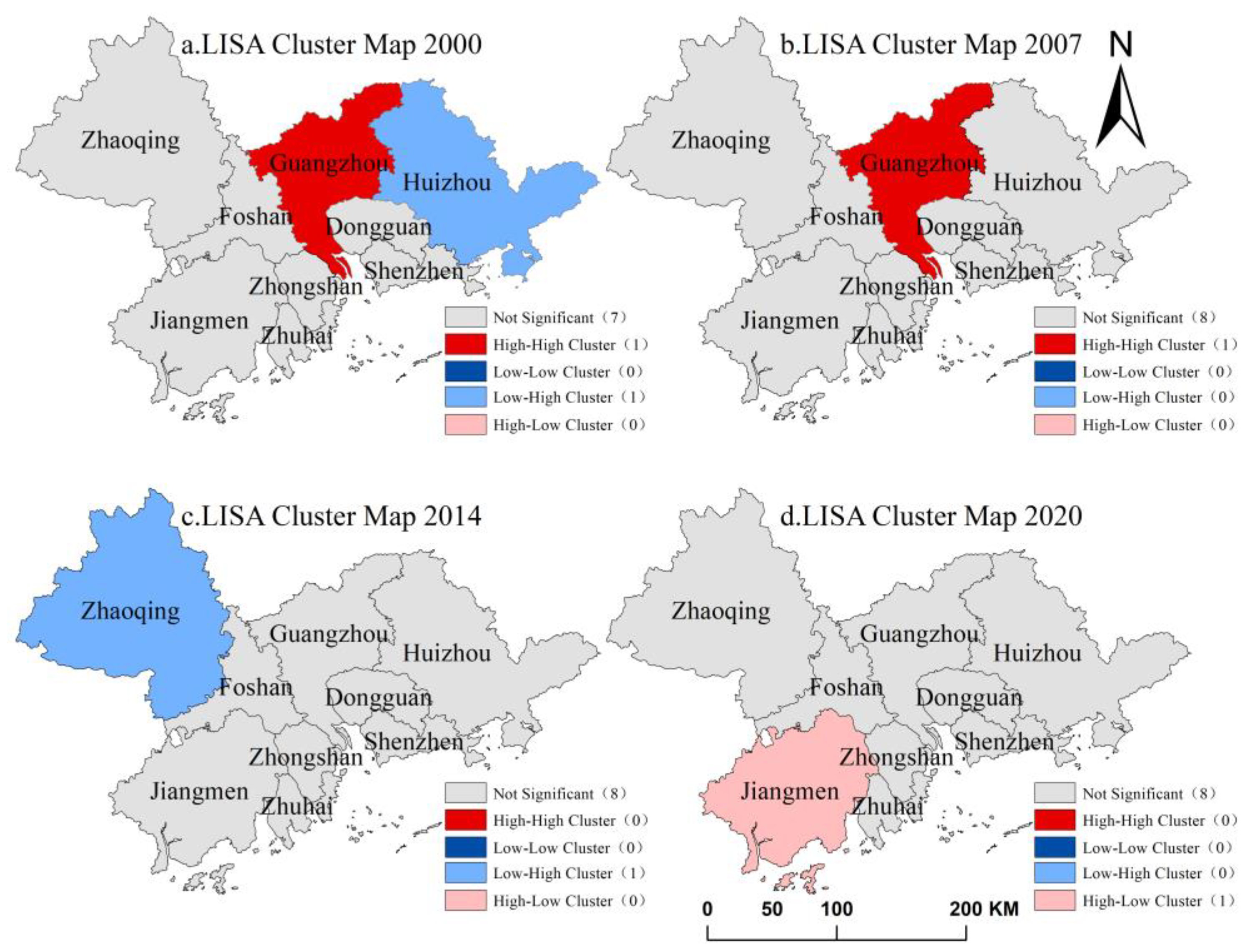
By calculating the global Moran’s I index for county-level cities in the Delta, we could only study and judge the spatial clustering relationship of overall spatial carbon emissions, while local Moran’s I index could well interpret the spatial clustering of carbon emissions in the Delta cities at municipal and county levels. Therefore, using spatial autocorrelation analysis function of OpenGeoDa and constructing the spatial weight coefficient matrix, local Moran’s I index was calculated for carbon emissions of municipal- and county-level cities in the Delta in 2000, 2007, 2014, and 2020. In addition, 999 random substitutions were carried out. The LISA cluster graph of Moran’s I index was obtained subsequently, and the graph is shown in Figure 4. The four phenomena in the graph represent high-value aggregation, high-value aggregation containing low-value anomaly, low-value aggregation, and low-value aggregation containing high-value anomaly, respectively. The carbon emission indicated that Gz in 2000 was a high-high-cluster city, while Hz was a low-high-cluster city. In 2007, carbon emissions of Hz increased gradually, and its cluster type became insignificant. In 2014, Zq City became a low-high-cluster city, consistent with its economic development and population density. In 2020, Jm transformed into a high-low-cluster city. On the whole, high carbon emission concentration area was distributed in Gz and Jm Cities, while a low carbon emission area was mainly concentrated in Zq City.
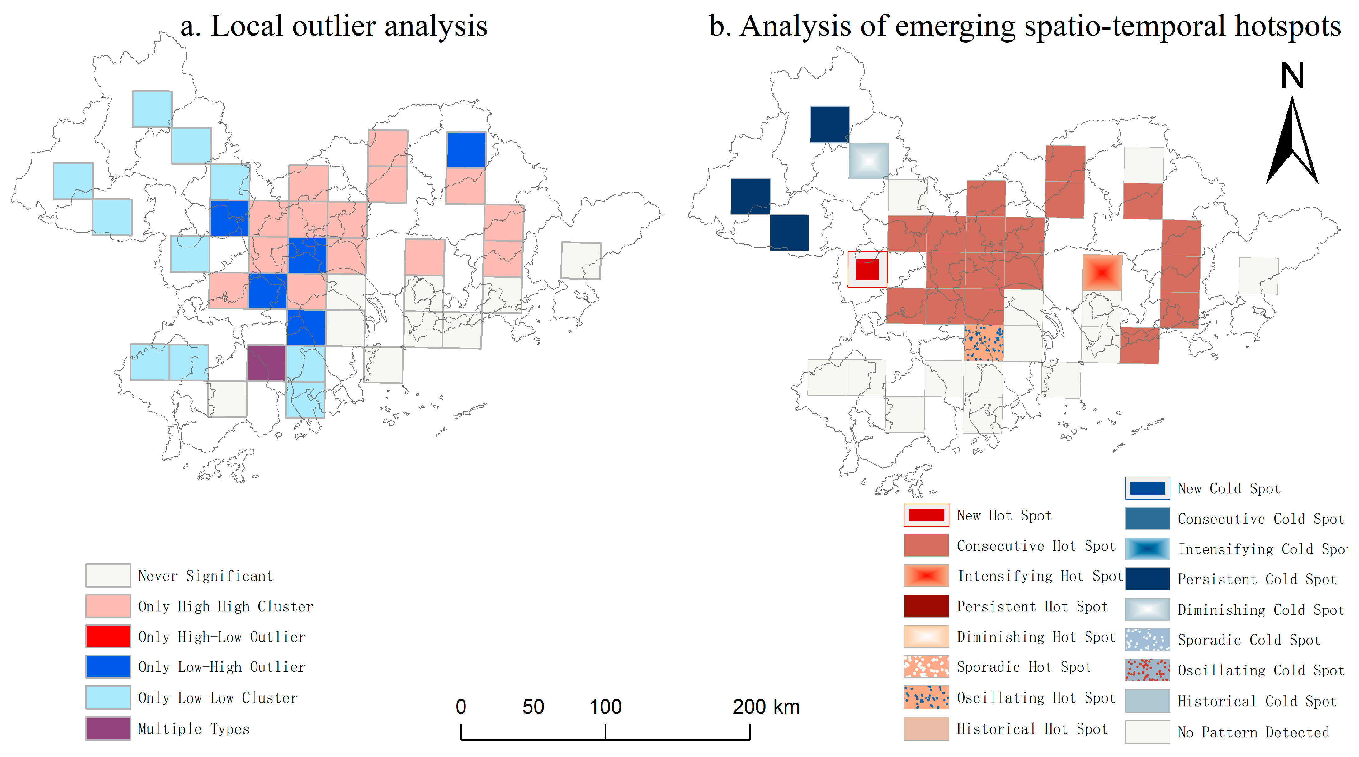
Figure 5 shows that in 2000, the high-high-value carbon emission cluster of county-level cities was mainly concentrated in Fs, Gz, and Dg Cities, while the low-low-value cluster was mainly concentrated in Fengkai, Huaiji, and Deqing Counties and Gaoyao District, consistent with the low level of economic development of Zq City and low level of development of county-level cities. Pengjiang, Chancheng, and Liwan Districts showed low values, including, however, abnormally high values. In 2020, the high-high carbon emission cluster of county-level cities shifted from the central region to the southeast of Hz, mainly to Huadu District, all districts of Hz City, and Dg City. The carbon emissions of all counties and regions of Gd and Fs Cities gradually became flat, with a balanced development of all regions and reduced carbon emission differences corresponding to a balanced urbanization development of Gd and Zs Cities. The low-low cluster included Huaiji County and Futian District; low values included high values distributed in Gaoming District, Longmen County, Pengjiang District, and Chancheng District; but there was no significant clustering feature in other areas. Although Huaji County was the only low-low cluster in Zq City, carbon emission of this city did not catch up with that of other municipal cities in the 20 years, reflecting that there was still a certain gap between this city and other cities in population and economic development.
The county-level local outliers are consistent with the spatial distribution of the city-level local outliers. For example, Zq has a low carbon emission level, while Gz has a high carbon emission level. However, the county-level local outliers are more detailed and precise in their spatial distribution. Therefore, the city-level local outliers can be used for large-scale spatial analysis, while the county-level local outliers can provide more refined suggestions for decision-makers in fine-grained decision-making processes.

4.3.2. County-Level STC-LOF and ES-THA

S-TC was the basis for STC-LOF and ES-THA. STC-LOF can detect the location of the cluster and the outliers that have statistically significant differences with their neighborhood in both space and time in the research area. The ES-THA is performed to add the element of time to detect the location of cold and hot spots in the spatio-temporal dimension. First, we extracted the carbon emission data of each county city center in the Delta, and created a spatio-temporal cube through the aggregation point of the county city center. STC-LOF and ES-THA of carbon emission of each county city in the Delta in the 20 years were conducted by taking one year as the neighborhood step and distance from city center as the step.
As shown in Figure 6a, through the STC-LOF, it was found that the carbon emissions of county-level cities in the Delta were not significant all the time. In particular, Nansha District, Zs City, Taishan City, Xiangzhou District, Guangming District, Bao‘an District, Futian District, Luohu District, Yantian District, Pingshan District, Longgang District, and Huidong County accounted for 26% of the total emissions in these county-level cities. In the 20 years, there was no abnormal value in space–time between the carbon emission of these regions and that of their surrounding regions, and their emissions were always in the stable range. In addition, Huadu District, Sanshui District, Baiyun District, Nanhai District, Yuexiu District, Tianhe District, Huangpu District, Panyu District, Shunde District, Chancheng District, Gaoxing District, Shunde District, Conghua District, Zengcheng District, Dg City, Boluo County, Huicheng District, and Huiyang District were all high-high clustering in the 20 years, accounting for 36% of the total emissions. Most high-carbon emission county-level cities were mainly concentrated in Gz in the new region of the Delta and Hz in the eastern region, consistent with the developed economy and dense population of Gz and Hz. There was no clustering of only high-low outliers for carbon emissions. The only low-high anomaly clusters included Dinghu District, Pengjiang District, Jianghai District, Liwan District, Haizhu District, and Longmen County. With the development of cities, the increase in or growth rate of carbon emissions of these cities was less than that of the surrounding cities. In other words, developing cities were surrounded by high carbon emissions of the surrounding cities. Only Huaiji County, Fengkai County, Guangning County, Sihui City, Deqing County, Duanzhou District, Enping City, Kaiping City, Doumen District, and Jinwan District had low-low clustering. IN addition, most county-level cities were distributed in Zq City, which corresponded to the Moran’s I index analysis and economic development of county-level cities. Compared with other county-level cities in the Delta, urban carbon emissions of these 10 county-level cities were in the low value region in the 20 years, and carbon emissions of the neighboring region were also in the low value region. Among the various types, there was one new association area, indicating that there were various types of abnormal clustering in the new association area in the 20 years. The STC-LOF could directly reflect the spatio-temporal clustering anomalies of carbon emissions in the county cities of the Delta in the 20 years, and also indirectly reflect the economic, population, and industrial changes in these 50 cities to a certain extent.
As shown in Figure 6b, the spatio-temporal hotspot analysis effectively showed complex spatial hotspots and development evolution rules of carbon emissions of county cities in the Delta in the 20 years. Five patterns were identified for the emissions, among which the high-power area was a new hotspot of carbon emissions from county cities in the Delta in 2020. Before this year, there was no statistically significant hot spot for carbon emissions in the high-power area, which indirectly reflected the rapid development of the high-power area in the recent years and an increase in its energy demand. The continuous hot spots were mainly distributed in the central and eastern parts of the Delta, including Dinghu District, Sanshui District, Gaoming District, Nanhai District, Chancheng District, Shunde District, Pengjiang District, Panyu District, Liwan District, Yuexiu District, Tianhe District, Huadu District, Huangpu District, Tianhe District, Haizhu District, Zengcheng District, Conghua District, Boluo County, Huicheng District, Huiyang District, Pingshan District, Yantian District, Yantian District, Luohu District, and Futian District. The results showed that these regions were the places with high carbon emissions for the 20 years, consistent with the STC-LOF and Moran’s I index analyses. There was one hot spot in Dg, indicating that Dg was a hot spot for the 20 years, the clustering intensity of carbon emissions increased every year, and the increase in carbon emissions was statistically significant. Huaiji, Fengkai, and Deqing Counties had permanent cold spots, which are located in the northwest of Zq. The presence of these cold spots indicated that 90% of the carbon emissions of these three cities were cold spots in the 20 years of development, and there was no obvious trend to show that clustering intensity of carbon emissions increased with time, consistent with the low-low clustering outliers of STC-LOF. Guangning County was one of the gradually decreasing cold spots, indicating that this county was a significant cold spot area for 90% of the time. However, the clustering intensity of carbon emissions showed a decreasing trend on the whole every year, with this intensity related to economic development and population growth, and the trend was statistically significant during the study period. The Jianghai region was the only oscillating hot spot, with the carbon emission in this region decreasing first and then increasing gradually.
On the whole, in the 20 years, the carbon emission of county cities in the Delta showed hot spots and high-value clusters in Gz, Sz, Zs, and Hz; the central and eastern parts of the Delta showed hot spot expansion and high-value clustering; and the northwest region of the Delta showed low value accumulation and cold-point expansion. Indirectly, these observations indicated that the overall gap of carbon emissions in the county-level cities was constantly expanding, and the clustering trend of high and low levels formed a fragmentation trend. In city-level urban units, carbon emissions were relatively clustered, and the gap was constantly narrowing.

4.3.3. Inequality of Carbon Emission Spatial Distribution at Multiple Scales

As shown in Table 4 and Table 5, PD and GDP were used as indicators, respectively, to establish the TL indices TP and TG of the overall carbon emission intensity of municipal cities. TL and contribution of per capita carbon emissions between municipal cities and within cities were represented by TbP, TwP, WbP, and WwP, and TL and the contribution of intra-city and inter-city carbon emission intensity was expressed by TbG, TwG, WbG, and WwG, respectively. WjP and WjG were used to represent contribution rates of each city in intra-city differences in per capita carbon emissions and carbon emission intensity, respectively.
In Table 4, it can be seen that the per capita carbon emission index between cities was above 0.2632 for the 20 years (it gradually dropped to 0.3613 from 2000 to 2020). The per capita carbon emissions in the Delta have always been different in space and region, but the difference showed a trend of fluctuation and decline. The Thiel index within each city was 10 times that of the among-city value, and the difference did not change with time. This observation indicated that per capita carbon emission and carbon emission intensity differences in cities in the Delta were mainly caused by urban differences, and the per capita carbon emission differences were increasing. The contribution of within-city differences was greater than the between-city differences in the city-level urban areas. However, from 2014 to 2020, the contribution of within-city differences was smaller than the between-city differences. The development of cities at the municipal level was unbalanced, and there were obvious differences in per capita carbon emissions. However, emission differences within cities was decreasing in the 20 years, while emission differences between cities gradually increased, which indirectly reflected the development imbalance and per capita differences between cities at the municipal level. The difference in Fs, Sz, Dg, Jm, and Hz Cities to the Delta was large, which was consistent with population distribution among the nine municipal cities. The average internal differences in Gz, Jm, and Zq were 0.4103, 0.5718, and 0.2402, respectively, indicating that the per capita carbon emissions of these three cities had the greatest impact on the Delta. In terms of contribution rate, intra-city contribution was obviously greater than inter-city contribution, but this gap was constantly narrowing.
As per Table 5, the Thiel index of carbon emission intensity of municipal cities increased from 0.3791 to 0.6391, indicating that difference in carbon emission intensity of municipal cities was continuously strengthened. Compared with the regional difference in per capita carbon emissions, the regional difference in carbon emission intensity was continuously enhanced, indicating that carbon emission of cities in the Delta had a high matching degree with GDP. The differences within cities were significantly greater than the differences between cities. The differences within Gz, Sz, Fs, and Zh were increasing, while those among other cities were narrowing, indicating that carbon emission intensity within these four cities was increasingly unbalanced. The contribution between cities was much greater than that within cities, and fluctuation of contribution was small, indicating that the impact of economic development between cities on carbon emissions was large and stable.
As shown in Figure 7, among the contribution rates of cities at municipal level, there were great differences in the impact of the nine cities on the carbon emission in the Delta. In terms of contribution rates of carbon emissions and carbon emission intensity per capita, the rates and intensity of Gz, Fs, Jm, Sz, and Hz were much higher than those of Zh, Dg, Zs, and Zq in the 20 years. Notably, Gz is the capital of Gd Province; Sz is a special economic zone, a national economic center city, and an international city; and Fs is the third largest city in the Province. Located in the hinterland of the Delta, Fs is in a superior geographical position. Factors such as this led to huge population, booming economy, and leading demand for energy of the above five cities. This might be the main reason for the huge differences in the per capita carbon emission and energy-intensity carbon emission contribution of these cities. The contribution of carbon emission intensity in Sz and Fs Cities was decreasing over time, largely due to full urbanization and balanced development. The increasing contribution of per capita carbon emission and carbon emission intensity in Hz and Zq, as indicated by the growing weight of their TL indices, suggesting significant population and economic development in these cities over the 20-year period. This may reflect notable differences in their economic development and energy consumption patterns compared to other cities or regions, leading to a gradual increase in their carbon emissions. It also implies that these cities may need to strengthen their environmental protection measures and carbon reduction efforts to mitigate their contribution to the overall carbon emissions.
In general, the Thiel index of per capita carbon emissions was decreasing in the 20 years, while the Thiel index of carbon emissions intensity was increasing. Specifically, the regional differences in per capita carbon emissions were greater than regional differences in carbon emissions before 2007. After 2007, regional differences in per capita carbon emissions was decreasing, while regional differences in carbon emission intensity was increasing. This indicated that the Delta was still facing the challenge of regional differences in the reduction in per capita carbon emissions. In terms of carbon emission contribution, contribution of per capita carbon emission was always higher than that of carbon emission intensity. The per capita carbon emission had a greater impact on total carbon emission of cities. In addition, the per capita carbon emission and the TL of carbon emission intensity of all municipal cities decreased from 2014 to 2020. This might be related to industrial restructuring, green urban development, revision of the Environmental Protection Law of the People’s Republic of China, and the 12th Five-Year Plan to strengthen energy conservation and emission reduction to achieve low-carbon development.

4.4. Analysis of Influencing Factors of Carbon Emission

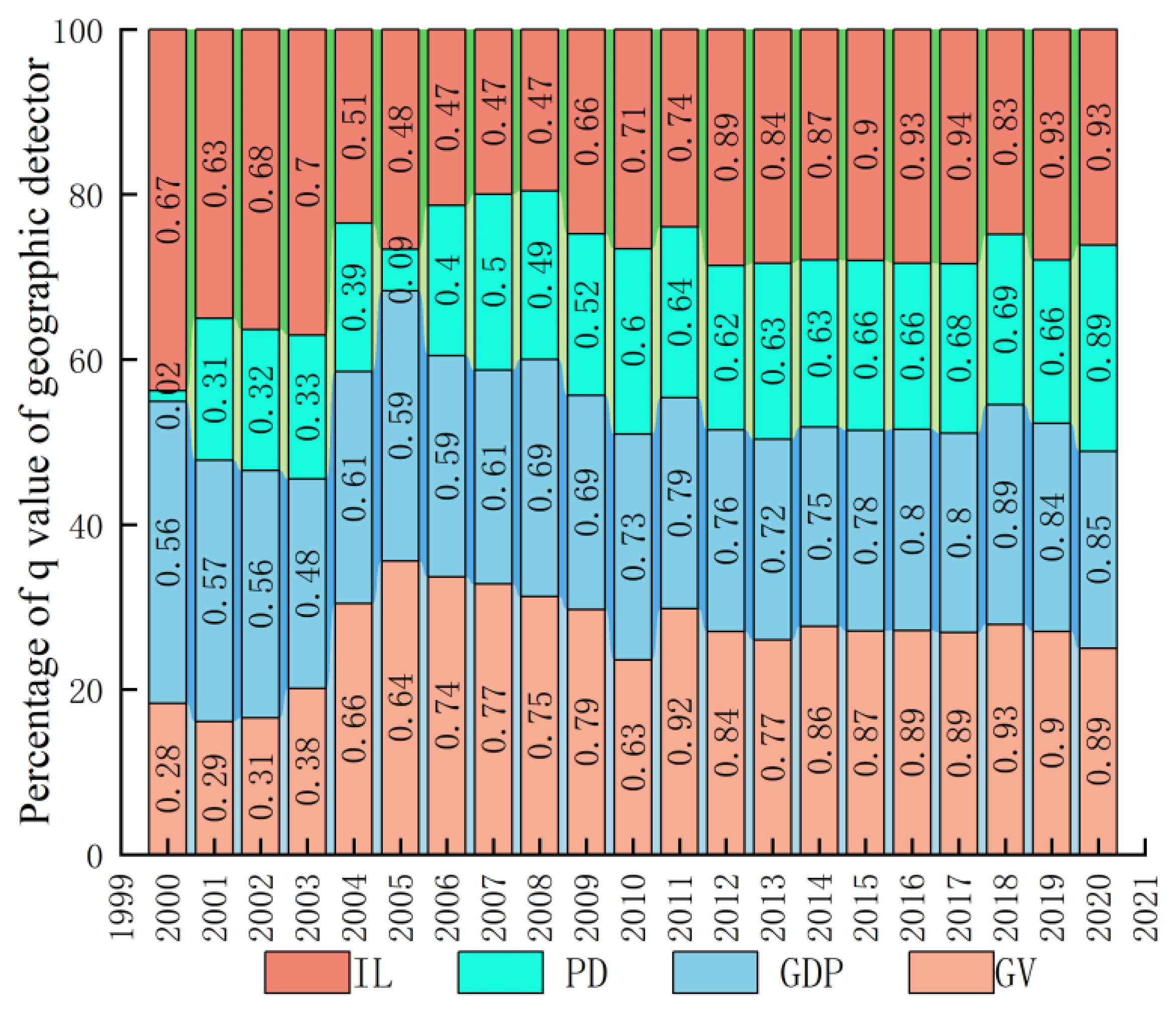
According to Section 3.6, to adapt the independent variable of the geographic detector as type variable, the impact factors were classified by natural discontinuous point classification method in ArcGIS 10.8. Accordingly, four factors including economic development level (GDP), population density (PD), number of enterprises above designated size (IL), and gross industrial output value (GV) were selected for the analysis based on [9,52]. The influencing factors of carbon emissions in the Delta were analyzed from the perspective of spatial differentiation using geographic detectors. The influence value q of a single factor on spatial heterogeneity of carbon emissions is shown in Figure 8.
From 2000 to 2020, carbon emissions of the Delta were mainly affected by level of economic development, number of enterprises above designated size, and total industrial output value. On the contrary, population density had the smallest effect on the emissions. The q value of gross industrial output value ranged from 0.28 at the beginning to 0.89 in 2020, and its explanatory power kept increasing, confirming that the gross industrial output was one of the leading factors. The explanatory power of GDP on spatial heterogeneity of carbon emissions was relatively stable, with the corresponding q value between 0.48 and 0.89. Economic development exerted a leading and stable effect on carbon emissions in the Delta. The q value of population density increased the fastest and was also in a stable range from 2006 to 2020, which was related to population distribution of county-level cities in the Delta. The population of the Delta was mainly concentrated in the economically developed and narrow central and eastern areas and coastal areas. Even though the northwestern area was vast, the population was attracted by the “siphon effect” of the central and eastern areas. This attraction led to a large population density gap in county-level cities. The number of enterprises above the scale occupied more than 50% in the early period of the study duration, which was related to China’s vigorous development of real economy and promotion of our economic development in 2000, but could only occupy about 25% in the late period. Adjustment of industrial institutions, improvement of energy utilization level, and innovation of science and technology greatly improved the efficiency of energy use during the study period. In addition, the concept of synergistic development between man and nature, implementation of carbon emission reduction measures, and transformation and development of enterprises weakened the explanatory power of the number of enterprises on carbon emissions. The influence of industrial output value increased from less than 20% to about 35% during the study period of 2000–2020. During 2000–2003, the industrial output value of the Delta was not high, while 2004–2010 was a period of rapid industrial development, which also resulted in a sharp increase in industrial energy demand and increased energy carbon emissions. In addition, the energy demand of industrial production accounted for a large part of urban energy, which could explain why the impact of industrial output on urban carbon emissions accounted for about 35% in the 20 years.
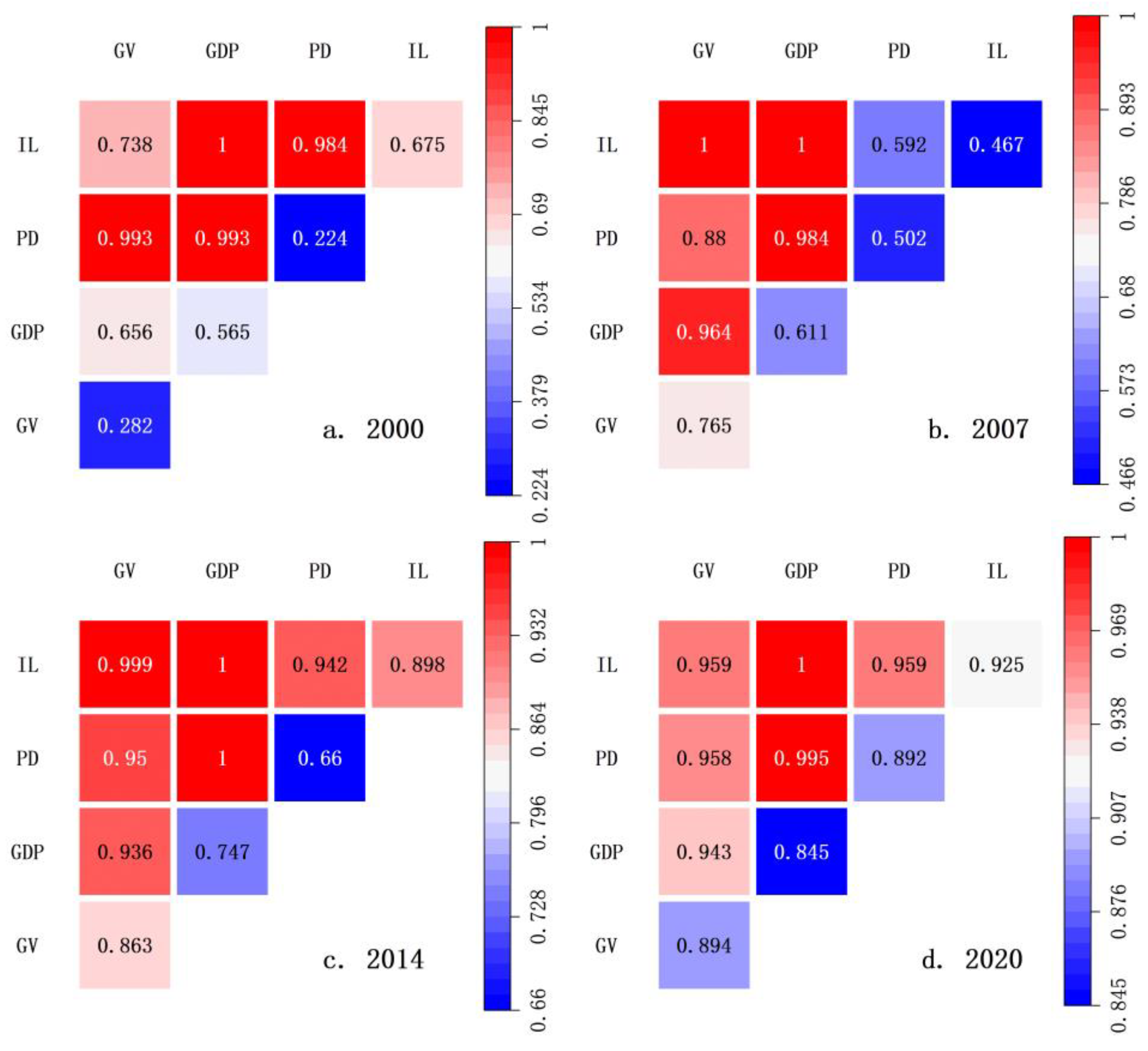
The interactive exploration and analysis of the four types of impact factors were carried out by a geographic detector, and the results are shown in Figure 9. The interaction of any two factors was a double-factor enhancement or a nonlinear enhancement, that is, the interaction of any two factors had a greater impact on carbon emissions of the Delta than that of a single factor [62], and the greater the value, the greater the impact. The interaction factor between population density and GDP was among the highest values from 2000 to 2020, indicating that growth of population and GDP greatly increased the demand for urban energy, that is, the impact on urban carbon emissions was among the highest. The value of population density as a single factor was not high, but in the interaction, the q value of population density increased significantly and was in the high-value area. Among the influences of single factors, factors with low q value greatly increased after interaction, which indicated that interaction of population density, GDP, number of enterprises, and total industrial output had a spatial superposition effect on carbon emissions in the Delta. In 2000, 2007, 2014 and 2020, the largest q values were GDP∩IL, IL∩GV\GDP, GDP∩IL\PD, and GDP∩IL, respectively. Therefore, the interaction between the number of enterprises above the scale and the GDP was the main driving force to promote carbon emission of the Delta. The single-factor q value of the total industrial output value was in the maximum line, while the q value of its interaction with various influencing factors was always at the low end. The development of emerging and high-precision technologies might require little energy consumption and bring great industrial output value, and the industrial development would be more energy efficient and environmentally friendly, and it is not particularly closely related to the number of large-scale enterprises and population density. The explanation of the interaction effect of total industrial output was not strong. As the population, economy, and science and technology center of Gd Province and an important region in the greater Delta region, the Delta will require more energy for future development. While maintaining development, policy adjustments can be implemented to the industrial structure, industrial distribution, and population distribution in order to achieve the goal of green development and low-carbon development and strive to achieve carbon neutrality as soon as possible.

5. Discussions

This study has some uncertainties and limitations.
First, when processing the NTL data, although we used the invariant target normalization method for calibration in Section 3.3, the uncertainty of the NTL data is increased due to factors such as the diffusion of lights, the terrain and geographical features of cities, and the limitations of the NTL data calibration methods. Even after calibration, there may still be outliers in the NTL data. In addition, in the era of big data, especially when obtaining data from satellite imagery, it is crucial to establish consistent time series. In this study, we referred to the method proposed by Zhong [42] and used a simple regression model to fit the NTL data. Although this method performed well in terms of error, it did not compare and analyze multiple fitting methods, which may have an impact on the accuracy. Therefore, in future research, we hope to develop improved calibration tools to extract NTL and conduct more in-depth research on NTL fitting methods.
Second, due to data availability limitations, the carbon emissions calculated in this study only include carbon emissions released from the consumption of 11 common fossil fuels. However, in reality, there are many other fossil fuels and human activities that release CO2 into the atmosphere, such as land use and cement production. Moreover, the influencing factors were limited to GDP, PD, IL, and GV. Therefore, in future research, it is necessary to comprehensively consider the sources of CO2 emissions and the factors that influence CO2 emissions in order to provide reference for the development of carbon reduction policies that are tailored to the specific circumstances of each region.
Third, the consumption of various energy sources, GDP, PD, IL, and GV were all obtained from the China City Statistical Yearbook. The accuracy of the yearbook data fundamentally affects the simulation accuracy. Shan [63] found that the reported data in the public yearbook has an error of ±10–15%, which may affect the accuracy of the carbon emission model. However, in our study, the model accuracy errors for provincial, city-level, and county-level areas were less than 10.7713%, 7.9615%, and 18.7385%, respectively. Therefore, the research results are stable and reliable.
Finally, our study mainly focuses on the spatial heterogeneity of carbon emissions in multi-level cities. However, does urban expansion, land use, and urban spatial structure affect carbon emissions? In this study, we did not conduct experiments on these factors. In the future, we will consider these factors and conduct further research on carbon emissions to contribute to the green development of cities around the world.

6. Conclusions and Policy Implications

Starting from basic data, this article uses easily obtainable NTL instead of statistical yearbook data to establish a carbon emission estimation model. Spatial autocorrelation, ES-THA, Tl, and geographic detector were used to analyze the spatial differentiation and the influencing factors of carbon emissions in cities at or above county level in the Delta. The results show that:
(1) As basic data, NTL effectively solves the problem of inconsistent statistical yearbook data and missing data for cities below the municipal level. It can estimate the carbon emissions of three-level cities, including the Delta, municipal and county-level cities, with a fitting accuracy of 99.3%. In the research of this article, the estimation error of the carbon emission model is below 18.7385%.
(2) The carbon emissions at the three levels of the cities, including municipal and county-level cities, were increasing from 2000 to 2020. Gaz and Fs were among the top emitters, while Zhi, JM, and Ze had lower carbon emissions. This is closely related to geographic location, economic development, industrial structure, and policies. The distribution of carbon emissions at the municipal and county levels has little difference. Therefore, the combination of macro municipal level and micro county level can be used for precise positioning of emission reduction.
(3) There was a strong spatial correlation between municipal and county-level carbon emissions in the Delta, and the spatial aggregation degree of carbon emissions at these two levels was increasing. At the county-level scale, county-level cities of Gz, Sz, and Hz were in the high-value cluster area, while county-level cities of Zq were in the low-value cluster area all year round. STC-LOF and ES-THA were performed on carbon emissions of the Delta spatio-temporal neighborhood by adding time conditions. It was determined via these analyses that carbon emission clusters in central, eastern, and northwestern regions were opposite to the hot spots. Although the carbon emissions in the northwestern region were increasing continuously, there was still a large gap with the other two regions. On the whole, the gap of carbon emissions in county-level cities was widening, and the clustering trend of high and low was forming a block trend. In city-level urban units, carbon emissions were more concentrated, and the gap was narrowing.
(4) The differences in per capita carbon emissions and carbon intensity of cities in the Delta were mainly caused by emission differences within cities. TL of per capita carbon emissions was decreasing in the 20 years, while that of carbon intensity was increasing. The Delta was still faced with the challenge of regional differences in the reduction in per capita carbon emissions.
(5) The factors affecting carbon emissions can be ranked in descending order as follows: economic development level, total industrial output value, number of industrial enterprises above designated size, and population density. The interactive effects of these four factors are far greater than the effects of a single factor. The spatial interaction of various factors is the main driving force behind the increase in carbon emissions. Among them, the impact of economic development is the strongest, and it can be used to adjust the weaker factors such as the number of industrial enterprises and population density, thereby weakening the dominant explanatory power of economic development and reducing carbon emissions.
Based on the key research conclusions, we put forward the following suggestions related to the realization path of the carbon neutrality target for the Delta.
(1) With the advancement of technology and the progress of the times, NTL remote sensing technology has become more mature and has advantages such as easy acquisition, large monitoring range, and high processing capability. In addition to DMSP-OLS and NPP-VIIRS, Wuhan University in China has independently developed the high-resolution remote sensing satellite LuoJia-1, which has a resolution of 130 m and higher sensitivity, enabling it to detect weak NTL signals and provide more comprehensive and accurate NTL features. The LuoJia-1 NTL sensor can obtain spectral information in multiple bands, including visible light and infrared bands, providing more comprehensive NTL features. Therefore, government departments should consider combining remote sensing technology with statistical data to establish a more refined and multi-scale carbon emission database which can facilitate dynamic monitoring of carbon emissions in various regions and cities. This can provide important data support and more systematic and differentiated solutions for the implementation of carbon reduction policies by relevant government departments, thereby helping China in its dual carbon actions at regional, provincial, city, and county scales.
(2) To strengthen carbon reduction efforts in key regions and industries in the Delta, it is important to focus on the development of cities with lower current carbon emissions. According to Section 3.5, cities in the eastern region are the main battlefield for carbon reduction and need to intensify their efforts. For example, in Gz, Sz, Fs, and Dg where there is high population density, it would be beneficial to relocate some residents to surrounding areas to relieve urban population pressure. In addition, high-carbon industries such as transportation and manufacturing in Gz, electronic information and manufacturing in Sz, manufacturing and textile industries in Dg, electronic information and aviation manufacturing industries in Zh, and steel, chemical, and building material industries in Fs need to be addressed through stricter regulations and management. It is also necessary to adjust the existing industrial structure, optimize the industrial layout, and raise the market access standards for high-carbon industries while vigorously developing efficient and low-carbon industries such as high-tech industries. However, relying solely on large cities with high carbon emissions to achieve energy conservation and emission reduction may not be enough. Therefore, it is important to focus on the development of smaller cities with lower carbon emissions, such as Zq and Jm. As agricultural cities in the south with abundant sunlight and water resources, Zq and Jg produce a large amount of agricultural waste that can be converted into biomass energy, and they can also develop solar, hydro, and biomass energy. Therefore, these smaller cities can actively promote the use of clean energy sources such as wind, solar, hydro, and biomass energy, and gradually shift towards an energy structure that emphasizes new energy development to promote green and low-carbon energy development.
(3) To achieve precise carbon reduction, it is necessary to clarify the functional orientation of each region, formulate differentiated carbon reduction measures and targets, and implement precise carbon reduction. The differences in per capita carbon emissions and carbon emission intensity in the Pearl River Delta urban agglomeration are mainly caused by the differences within cities rather than those between cities, with greater contribution from within city-level areas than between them. Moreover, within cities, population has a higher contribution than economic factors do. Therefore, a combined policy approach at the city and county level can be implemented to optimize policies based on the size of the contribution of different factors in different cities. In areas where there is little difference in the spatial distribution of carbon emissions between city-level and county-level areas, macro city-level policies should be the main focus, with micro county-level policies as a supplement. For areas with significant differences in spatial distribution of carbon emissions, specific carbon reduction measures and targets should be developed.

Supplementary Materials

NTL, administrative boundary data, carbon emission statistics and other socio-economic data supporting the conclusions of this article are available at: https://ngdc.noaa.gov/eog/viirs/download_ut_mos.html, http://www.ngcc.cn/ngcc/, http://www.stats.gov.cn/sj/zgtjnj/.

Author Contributions

S.Z. and Y.L. created and designed the research, S.Z. analyzed the data, Y.L. and G.Z. contributed to the design of this research. All authors have read and agreed to the published version of the manuscript.

Funding

This work was supported by the National Natural Science Foundation of China (Grant No. 42101393).

Institutional Review Board Statement

Not applicable.

Informed Consent Statement

Not applicable.

Data Availability Statement

No new data were created or analyzed in this study. Data availability is not applicable as no datasets were generated or analyzed during the current study.

Conflicts of Interest

The authors declare that they have no competing interest.

References

  1. Harvey, L.D.D. Allowable CO2 concentrations under the United Nations Framework Convention on Climate Change as a function of the climate sensitivity probability distribution function. Environ. Res. Lett. 2007, 2, 14001. [Google Scholar] [CrossRef]
  2. Aichele, R.; Felbermayr, G. The Effect of the Kyoto Protocol on Carbon Emissions. J. Policy Anal. Manag. 2013, 32, 731–757. [Google Scholar] [CrossRef]
  3. Dimitrov, R.S. Inside UN Climate Change Negotiations: The Copenhagen Conference. Rev. Policy Res. 2010, 27, 795–821. [Google Scholar] [CrossRef]
  4. Qinghua, L.; Peng, L.; Bin, R.R.; Shengbin, L.; Xiaoping, Z.; Cheng, Z.; Wang, Y.; Wu, L.; Yao, H. Carbon Emission Characteristics of Resource-Based Cities in China. Iran. J. Sci. Technol. Trans. Civ. Eng. 2022, 46, 4579–4591. [Google Scholar]
  5. Wang, Y.; Zhao, H. The impact of China’s carbon trading market on regional carbon emission efficiency. China Popul. Resour. Environ. 2019, 29, 50–58. [Google Scholar]
  6. Wang, Y.; Wang, M.; Liu, L.; Li, S.; Lin, Y. Analyzing the spatiotemporal differences of carbon emission in the PearlRiver Delta using DMSP/OLS nighttime light images. J. Remote Sens. 2022, 26, 1824–1837. [Google Scholar]
  7. Wang, X.; Wu, J.; Wang, Z.; Jia, X.; Bai, B. Accounting and Characteristics Analysis of CO2 Emissions in Chinese Cities. Chin. J. Urban Environ. Stud. 2020, 8, 2050004. [Google Scholar] [CrossRef]
  8. Bao, S.; Tian, L.; Wang, J. Trend Forecast of Energy Production and Consuumption in China and Research of Carbon Emissions. J. Nat. Resour. 2010, 25, 1248–1254. [Google Scholar]
  9. Zhao, X.; Peng, J.; Hu, Y.; Zhang, Z. Spatial-temporal pattern and influence factors of county carbon emissions in Hunan Province based on nightlight data. Ecol. Sci. 2022, 41, 91–99. [Google Scholar]
  10. Zhou, X. Carbon Dioxide Emissions Estimation and Spatio-Temporal Distribution of Gd Province Based on Nighttime Light Data; Chengdu University of Technology: Chengdu, China, 2018. [Google Scholar]
  11. Li, Y.; Sheng, Q.; Dai, J. Spatio-temporal characteristics of carbon emission in Beijing-Tianjin-Hebei urban agglomeration derived from integrated DMSP-OLS and NPP-VIIRS nighttime light data. J. Environ. Eng. Technol. 2023. Available online: https://x.cnki.net/kcms/detail/detail.aspx?filename=HKWZ202302001&dbcode=CJFD&dbname=CJFDTEMP&v=sZmz0fHCQ4uDUSBUyvD75d3Iim1RLQqCwq0c1YmsO72e2AO3cFhoVjGCc4tWE5ca (accessed on 12 April 2023).
  12. Xu, L. A Study on the Spatial-Temporal Pattern and Influence Factors of Prefecture-Level Cities Resident’s per Capita Carbon Emissions in China; Lanzhou University: Lanzhou, China, 2019. [Google Scholar]
  13. Liu, Y.; Yan, B.; Zhou, Y. Urbanization, economic growth, and carbon dioxide emissions in China: A panel cointegration and causality analysis. J. Geogr. Sci. 2015, 26, 131–152. [Google Scholar] [CrossRef]
  14. Wang, W.; Kuang, Y.; Huang, N. Spatial Autocorrelation Analysis on Energy-Related CarbonEmission in Gd. Environ. Sci. Technol. 2014, 37, 180–187+193. [Google Scholar]
  15. Hu, X.; Jiao, W.; Chen, X.; Pang, J. The Dynamics and Spatial Differentiation Research of Carbon Emission from Energy Consumption in Henan Province. Areal Res. Dev. 2017, 36, 147–152. [Google Scholar]
  16. Ma, C.; Zou, S.; Zhao, J.; Wen, Q.; Mi, W. Temporal-Spatial Difference Analysis of Carbon Emission from EnergyConsumption and Its Regional Type Division in Northwest China. Econ. Geogr. 2016, 36, 162–168. [Google Scholar]
  17. Xu, Y.; Zhang, W.; Wang, J.; Ji, S.; Wang, C.; Streets, D.G. Investigating the spatially heterogeneous impacts of urbanization on city-level industrial SO2 emissions: Evidence from night-time light data in China. Ecol. Indic. 2021, 133, 108430. [Google Scholar] [CrossRef]
  18. Yang, X.; Liu, X. Accuracy analysis of inverting provincial-level carbon emissions from night-time light data in China: Comparison based on international carbon emission data. In IOP Conference Series: Earth and Environmental Science; IOP Publishing: Bristol, UK, 2020; Volume 601, p. 012046. [Google Scholar]
  19. Xu, W.-H.; Xie, Y.-L.; Ji, L.; Cai, Y.-P.; Yang, Z.-F.; Xia, D.-H. Spatial-temporal evolution and driving forces of provincial carbon footprints in China: An integrated EE-MRIO and WA-SDA approach. Ecol. Eng. 2022, 176, 106543. [Google Scholar] [CrossRef]
  20. Li, J.; Huang, X.; Chuai, X.; Yang, H. The impact of land urbanization on carbon dioxide emissions in the Yangtze River Delta, China: A multiscale perspective. Cities 2021, 116, 103275. [Google Scholar] [CrossRef]
  21. Zhou, P.; Wang, M. Carbon dioxide emissions allocation: A review. Ecol. Econ. 2016, 125, 47–59. [Google Scholar] [CrossRef]
  22. Wang, L.; Wang, S.; Yi, Z.; Liu, W.; Hou, Y.; Zhu, J.; Wang, F. Mapping population density in China between 1990 and 2010 using remote sensing. Remote Sens. Environ. 2018, 210, 269–281. [Google Scholar] [CrossRef]
  23. Elvidge, C.D.; Baugh, K.E.; Kihn, E.A.; Kroehl, H.W.; Davis, E.R.; Davis, C.W. Relation between satellite observed visible-near infrared emissions, population, economic activity and electric power consumption. Int. J. Remote Sens. 1997, 18, 7. [Google Scholar] [CrossRef]
  24. Doll CN, H.; Muller, J.P.; Elvidge, C.D. Night-time Imagery as a Tool for Global Mapping of Socioeconomic Parameters and Greenhouse Gas Emissions. Ambio A J. Hum. Environ. 2000, 29, 157–162. [Google Scholar] [CrossRef]
  25. Ghosh, T.; Elvidge, C.D.; Sutton, P.C.; Baugh, K.E.; Ziskin, D.; Tuttle, B.T. Creating a Global Grid of Distributed Fossil Fuel CO2 Emissions from Nighttime Satellite Imagery. Energies 2010, 3, 1895–1913. [Google Scholar] [CrossRef]
  26. Raupach, M.R.; Rayner, P.J.; Paget, M. Regional variations in spatial structure of nightlights, population density and fossil-fuel CO2 emissions. Energy Policy 2010, 38, 4756–4764. [Google Scholar] [CrossRef]
  27. Meng, L.; Graus, W.; Worrell, E.; Huang, B. Estimating CO2 (carbon dioxide) emissions at urban scales by DMSP/OLS (Defense Meteorological Satellite Program’s Operational Linescan System) nighttime light imagery: Methodological challenges and a case study for China. Energy 2014, 71, 468–478. [Google Scholar] [CrossRef]
  28. Liu, Y.; Wang, Y.; Peng, J.; Du, Y.; Liu, X.; Li, S.; Zhang, D. Correlations between Urbanization and Vegetation Degradation across the World’s Metropolises Using DMSP/OLS Nighttime Light Data. Remote Sens. 2015, 7, 2067–2088. [Google Scholar] [CrossRef]
  29. Alahmadi, M.; Atkinson, P.M. Three-fold urban expansion in Saudi Arabia from 1992 to 2013 observed using calibrated DMSP-OLS night-time lights imagery. Remote Sens. 2019, 11, 2266. [Google Scholar] [CrossRef]
  30. Su, Y.; Chen, X.; Li, Y.; Liao, J.; Ye, Y.; Zhang, H.; Huang, N.; Kuang, Y. China’s 19-year city-level carbon emissions of energy consumptions, driving forces and regionalized mitigation guidelines. Renew. Sustain. Energy Rev. 2014, 35, 231–243. [Google Scholar] [CrossRef]
  31. Shi, K.; Chen, Y.; Yu, B.; Xu, T.; Chen, Z.; Liu, R.; Li, L.; Wu, J. Modeling spatiotemporal CO2 (carbon dioxide) emission dynamics in China from DMSP-OLS nighttime stable light data using panel data analysis. Appl. Energy 2016, 168, 523–533. [Google Scholar] [CrossRef]
  32. Chand, T.K.; Badarinath, K.; Elvidge, C.; Tuttle, B. Spatial characterization of electrical power consumption patterns over India using temporal DMSP-OLS night-time satellite data. Int. J. Remote Sens. 2009, 30, 647–661. [Google Scholar] [CrossRef]
  33. Elvidge, C.D.; Ziskin, D.; Baugh, K.E.; Tuttle, B.T.; Ghosh, T.; Pack, D.W.; Erwin, E.H.; Zhizhin, M. A fifteen year record of global natural gas flaring derived from satellite data. Energies 2009, 2, 595–622. [Google Scholar] [CrossRef]
  34. Wang, S.; Su, Y.; Zhao, Y. Regional inequality, spatial spillover effects and influencingfactors of China’s city-level energy-related carbon emissions. Acta Geogr. Sin. 2018, 73, 414–428. [Google Scholar]
  35. Xia, S.; Shao, H.; Wang, H.; Xian, W.; Shao, Q.; Yin, Z.; Qi, J. Spatio-Temporal Dynamics and Driving Forces of Multi-Scale CO2 Emissions by Integrating DMSP-OLS and NPP-VIIRS Data: A Case Study in Beijing-Tianjin-Hebei, China. Remote Sens. 2022, 14, 4799. [Google Scholar] [CrossRef]
  36. Shi, K.; Yun, C.; Li, L.; Huang, C. Spatiotemporal variations of urban CO2 emissions in China: A multiscale perspective. Appl. Energy 2018, 211, 218–229. [Google Scholar] [CrossRef]
  37. Lu, H.; Liu, G. Spatial effects of carbon dioxide emissions from residential energy consumption: A county-level study using enhanced nocturnal lighting. Appl. Energy 2014, 131, 297–306. [Google Scholar] [CrossRef]
  38. Liu, X.; Yang, X. The Accuracy of Nighttime Light Data to Estimate China’s Provincial Carbon Emissions: A Comparison with Carbon Emissions Allocated by International Carbon Database. Remote Sens. Technol. Appl. 2022, 37, 319–332. [Google Scholar]
  39. Lan, T.; Shao, G.; Tang, L.; Xu, Z.; Zhu, W.; Liu, L. Quantifying Spatiotemporal Changes in Human Activities Induced by COVID-19 Pandemic Using Daily Nighttime Light Data. IEEE J. Sel. Top Appl. Earth Obs. Remote Sens. 2021, 14, 2740–2753. [Google Scholar] [CrossRef]
  40. Xu, G.; Xiu, T.; Li, X.; Liang, X.; Jiao, L. Lockdown induced night-time light dynamics during the COVID-19 epidemic in global megacities. Int. J. Appl. Earth Obs. Geoinf. 2021, 102, 102421. [Google Scholar] [CrossRef]
  41. Cao, Z.; Wu, Z.; Kuang, Y.; Huang, N. Correction of DMSP/OLS Night-time Light Images and Its Application in China. J. Geo-Inf. Sci. 2015, 17, 1092–1102. [Google Scholar]
  42. Zhong, X. Research on Correction and Fusion of DMSP/OLS and NPP/VIIRS Nighttime Light Data; China University of Mining and Technology: Beijing, China, 2022. [Google Scholar]
  43. Su, Y. Study on the Carbon Emissions from Energy Consumption in China Using DMSP/OLS Night Light Imageries; Institute of Geochemistry, Chinese Academy of Sciences: Guizhou, China, 2015. [Google Scholar]
  44. Gu, Y.; Qiao, X.; Fan, L.; Guan, Z.; Feng, D.; Gao, Y. Spatial analysis of carbon emissions from region energy consumption based on night light data. Sci. Surv. Mapp. 2017, 42, 140–146. [Google Scholar]
  45. Wu, N.; Shen, L.; Zhong, S. Spatio-temporal Pattern of Carbon Emissions based on Nightlight Data of the Shanxi-Shaanxi-Inner Mongolia Region of China. J. Geo-Inf. Sci. 2019, 21, 1040–1050. [Google Scholar]
  46. Chen, G. Spatiotemporal Evolution Pattern and Influencing factors of Energy Consumption Carbon Emissions in Lanzhou-Xining City Group; Lanzhou University of Finance and Economics: Lanzhou, China, 2022. [Google Scholar]
  47. Pinto, E.P.; Pires, M.A.; Matos, R.S.; Zamora, R.R.M.; Menezes, R.P.; Araújo, R.S.; de Souza, T.M. Lacunarity exponent and Moran index: A complementary methodology to analyze AFM images and its application to chitosan films. Phys. A Stat. Mech. Its Appl. 2021, 581, 126192. [Google Scholar] [CrossRef]
  48. Wang, S. Remote Sensing Monitoring and Temporal and Spatial Analysis of Forest Change Characteristics in Southwest China in Recent 20 Years; Southwest University: Chongqing, China, 2022. [Google Scholar]
  49. Cuba, N.; Sauls, L.A.; Bebbington, A.J.; Bebbington, D.H.; Chicchon, A.; Marimón, P.D.; Diaz, O.; Hecht, S.; Kandel, S.; Osborne, T.; et al. Emerging hot spot analysis to indicate forest conservation priorities and efficacy on regional to continental scales: A study of forest change in Selva Maya 2000–2020. Environ. Res. Commun. 2022, 4, 71004. [Google Scholar] [CrossRef]
  50. Shan, B.; Zhang, Z.; Chen, Y.; Yu, X.; Fan, W.; Lv, Y. Analysis Methods of Spatio-temporal Patterns and Its Empirical Applications——A Case Study of Manufacturing Industry of Shandong Province. J. Geomat. Sci. Technol. 2021, 38, 624–630+638. [Google Scholar]
  51. Cai, H.; Chen, S.; Pan, K. Analysis on Spatial Imbalance and Dynamic Evolution of Carbon Lock-in: Taking Jiangsu Province as an Example. J. Zhejiang Shuren Univ. 2022, 22, 50–59+75. [Google Scholar]
  52. Song, M.; Zou, S. Regional Differences, Convergence and Influencing Factors of Carbon Emissions Efficiency in the Yellow River Basin. Yellow River 2022, 44, 6–12+56. [Google Scholar]
  53. Cui, Y.; Khan, S.U.; Deng, Y.; Zhao, M. Spatiotemporal heterogeneity, convergence and its impact factors: Perspective of carbon emission intensity and carbon emission per capita considering carbon sink effect. Environ. Impact Assess. Rev. 2022, 92, 106699. [Google Scholar] [CrossRef]
  54. Wang, G.; Liao, M.; Jiang, J. Research on Agricultural Carbon Emissions and Regional Carbon Emissions Reduction Strategies in China. Sustainability 2020, 12, 2627. [Google Scholar] [CrossRef]
  55. Shao, S.; Zhang, K.; Dou, J. Comparisons on the Income Measurements in Chinese Household Survey Data. Manag. World 2019, 35, 36–60+226. [Google Scholar]
  56. Ma, T.; Zhou, C.; Pei, T.; Haynie, S.; Fan, J. Responses of Suomi-NPP VIIRS-derived nighttime lights to socioeconomic activity in China’s cities. Remote Sens. Lett. 2014, 5, 165–174. [Google Scholar] [CrossRef]
  57. Liu, X.; Gao, C.; Song, Y.; Zhang, Y.; Su, Q.; Tian, Y. Temporal-spatial carbon emission patterns caused by fossil energy consumption at the city level in Hunan Province, China and the factors driving their composition. Acta Ecol. Sin. 2017, 37, 2476–2487. [Google Scholar]
  58. Zhao, X. System Analysis and Regulation of Energy Consumption Carbon Emissions of Hunan Province; Hunan Normal University: Changsha, China, 2014. [Google Scholar]
  59. Yang, S.; Zhang, Y.; Geng, Y. An LMDI-based investigation of the changes in carbon emissions of the transportation sector in the Yangtze River Economic. China Environ. Sci. 2022, 42, 4817–4826. [Google Scholar]
  60. Wang, S.; Huang, Y. Spatial spillover effect and driving forces of carbon emission intensity at city level in China. Acta Geogr. Sin. 2019, 74, 1131–1148. [Google Scholar] [CrossRef]
  61. Wang, J.; Xu, C. Geodetector:Principle and prospective. Acta Geogr. Sin. 2017, 72, 116–134. [Google Scholar]
  62. Wang, X.; Zhang, X.; Wang, Y.; Yan, Y. Spatial evolution and driving force analysis of ecological-production-living spaces on the Loess Plateau. J. Anhui Agric. Univ. 2022, 49, 112–121. [Google Scholar]
  63. Shan, Y.; Guan, D.; Liu, J.; Mi, Z.; Liu, Z.; Liu, J.; Schroeder, H.; Cai, B.; Chen, Y.; Shao, S.; et al. Methodology and applications of city level CO2 emission accounts in China. J. Clean. Prod. 2017, 161, 1215–1225. [Google Scholar] [CrossRef]
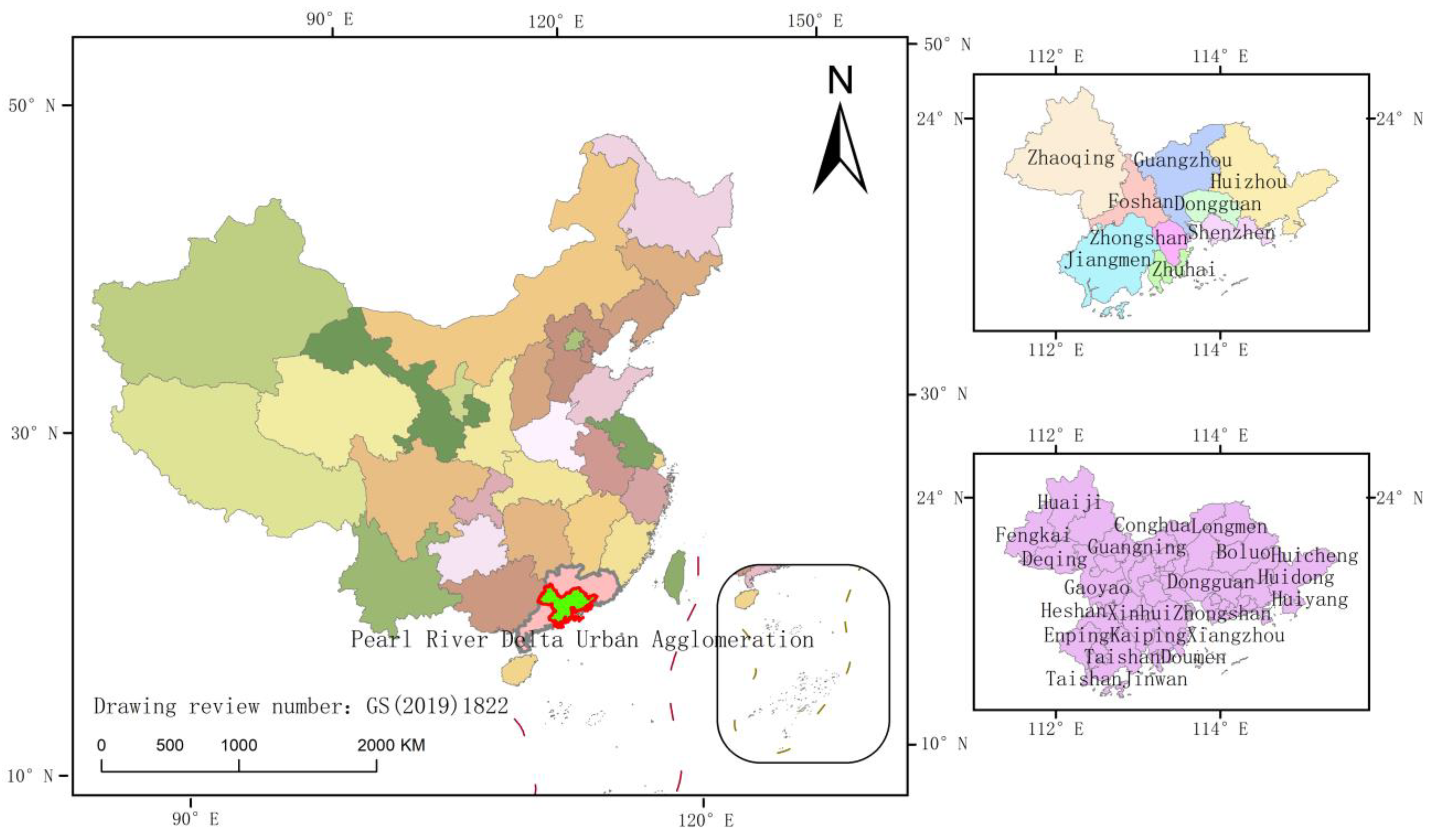
Figure 1. Study Area. Note: Dg and Zs are all urbanized and have not been divided into county-level cities.
Sustainability 15 08234 g001
Figure 2. Fitting effect and 20-year- change in carbon emissions in the Delta.
Sustainability 15 08234 g002
Figure 3. Spatial simulation of carbon emissions in county-level cities.
Sustainability 15 08234 g003
Figure 4. Moran’s I index LISA cluster map of carbon emissions in the cities of the Delta.
Sustainability 15 08234 g004
Figure 5. Moran’s I index LISA cluster map of carbon emissions of county-level cities in the Delta.
Sustainability 15 08234 g005
Figure 6. STC-LOF and ES-THA.
Sustainability 15 08234 g006
Figure 7. Contribution rate of Tl of carbon emissions of municipal cities.
Sustainability 15 08234 g007
Figure 8. Factor detector (q value) result.
Sustainability 15 08234 g008
Figure 9. Interactive detector results.
Sustainability 15 08234 g009
Table 1. Conversion coefficient and carbon emission coefficients of converted standard coal.
TypeConversion Coefficient of Standard Coal (t/t)Carbon Emission Factor/(104 t/104 t)
Coal0.71430.7559
Coke0.97140.8550
Crude oil1.42860.5857
Gasoline1.47140.5538
Kerosene1.47140.5714
Diesel1.45710.5921
Fuel oil1.42860.6185
Liquefied petroleum gas1.61980.5042
Natural gas1.33000.4483
The thermal34.12000.6700
Electric power0.34500.2720
“t/t” can be translated as “tons of standard coal per ton”, which represents the standardized reference coefficient of energy consumption per unit. “(104 t/104 t)” can be translated as “tons of carbon per ton of standard coal”, which represents the carbon emissions per unit of standard coal. The units of conversion coefficients for natural gas, electricity and heat are kg/m3, kg/(kW·h) and kg/(106 kj), respectively.
Table 2. Error in the three-level city carbon emission model.
Region/Year199719981999 Mean
Gd9.4178%5.1477%10.7713% 8.4456%
2000200720142020
Gz7.1487%3.2479%6.7489%7.1678%6.5783%
Sz6.8972%4.0125%7.1148%6.9715%6.7490%
Zq7.9615%7.3103%7.7214%7.3872%7.3451%
Dg5.4179%6.1024%7.9015%6.1078%6.1324%
2000200720142020
County average15.4781%9.4713%17.1329%18.7385%15.4552%
Table 3. Moran’s I index of carbon emissions of county-level cities in the Delta.
ScaleVariable20002003200620092012201520182020
MunicipalMoran’s I0.05910.08180.11220.11870.12740.15520.14470.1391
Z1.01871.20441.39051.43131.51201.11490.99480.9241
P0.164010.12240.09430.08890.07750.13720.16300.1775
County levelMoran’s I0.22240.24760.27020.27320.2710.2870.3140.323
Z2.55403.07593.30973.37643.34033.46763.70423.5020
P0.01390.00520.00330.00240.00120.00170.00140.0033
Table 4. TL of city level cities based on per capita carbon emissions.
TimeTPTbPwbP
GzSzZhFsHzDgZsJmZq
20000.5600
0.2632
0.4775
0.3613
0.05800.07700.03340.19450.04150.04820.01680.10860.00460.4042
20070.01040.02520.02380.07830.07550.05380.02030.02130.00570.3957
20140.04570.03110.06110.08790.12920.04890.02020.06380.02360.3842
20200.03210.05670.03320.02290.16760.04810.02210.10410.04220.5842
TwPwwP
GzSzZhFsHzDgZsJmZq
20000.57470.26380.02180.03360.02330.00000.00001.12820.21930.5958
20070.35520.22060.06070.07410.04580.00000.00000.02780.24470.6043
20140.36210.13940.11460.10000.07220.00000.00001.08480.28590.6158
20200.34820.14070.12170.12870.01870.00000.00000.04620.21100.4158
Table 5. TL among municipal cities based on carbon emission intensity.
TimeTGTbGwbG
GzSzZhFsHzDgZsJmZq
20000.37910.08070.15570.01080.11050.09690.02790.01130.06510.06390.6145
20070.49530.00970.12020.02200.05380.16440.04290.01620.10480.10440.5646
20140.54740.00500.10690.03580.03640.14260.04180.01890.13490.08020.4881
20200.63910.04260.11260.02540.03450.23520.03900.01130.18770.11580.6149
TwGWwG
GzSzZhFsHzDgZsJmZq
20000.29470.28050.01860.03100.10460.00000.00000.03830.10060.3855
20070.52640.16000.11420.08550.25060.00000.00000.04260.08620.4354
20140.51540.28430.21540.09050.50410.00000.00000.05200.11160.5119
20200.55560.25720.28960.10030.20690.00000.00000.07840.12570.3851
Disclaimer/Publisher’s Note: The statements, opinions and data contained in all publications are solely those of the individual author(s) and contributor(s) and not of MDPI and/or the editor(s). MDPI and/or the editor(s) disclaim responsibility for any injury to people or property resulting from any ideas, methods, instructions or products referred to in the content.