Abstract
In-vehicle traffic lights (IVTLs) have been identified as a potential means of eco-driving. However, the extent to which they influence driving characteristics in the event of obstructed on-road traffic lights (ORTLs) has yet to be fully examined. Firstly, the situation of partially deployed IVTLs in both vehicles was analyzed to identify the factors that affect driving characteristics. Through the following distance model, relative vehicle speed, acceleration and deceleration, and following distance were recognized as the contributing factors. The evaluation indicators for driving characteristics were thereby further established. Then, a hardware-in-the-loop simulation platform was built using PreScan 8.5-MATLAB/Simulink R2018b joint simulation software and a Logitech G29 device. IVTLs were implemented using modules in the joint simulation software. Finally, under the scenarios of obstructed ORTLs and various deployment conditions of IVTLs, the original data were collected from 50 experimental subjects with simulated driving. The subjects included 25 males and 25 females, all of whom were non-professional drivers, with ages ranging from 20 to 40 years old. The conclusion was reached that IVTLs could improve driving comfort by approximately 10% in sunny weather (p = 0.008 < 0.05, p = 0.023 < 0.05; p = 0.046 < 0.05, p = 0.001 < 0.05), driving maneuverability by approximately 30% in foggy weather (p = 0.033 < 0.05), and driving safety by approximately 50% in the ORTLs obstructed by a truck scenario (p = 0.019 < 0.05). In general, even if only one vehicle was equipped with IVTLs, certain gain effects on the driving characteristics of both vehicles could still be provided.
1. Introduction
The dynamics of driving characteristics are shaped by the interplay between intricacies of road conditions and capabilities of advanced driver-assistance systems (ADASs). Road conditions include natural factors and the road environment. Natural factors encompass a diverse array of meteorological conditions, including but not limited to bright and sunny weather, dense and misty weather, inclement and rainy weather, and tempestuous sandstorms. The road environment encompasses a multifaceted array of elements, such as traffic congestion, vehicular collisions, and ongoing construction projects. The technologies of ADASs include lane-keeping assist systems and in-vehicle traffic lights (IVTLs). All of the above collectively shape the driving experience.
1.1. The Impact of Road Conditions on Driving Characteristics
Historically, scholars have focused more intently on studying the nuances of driving characteristics during inclement weather conditions, as opposed to during clear and sunny weather. The authors in [1] meticulously expounded upon the micro-mechanisms of how abnormal weather conditions impact transportation and proffered a method for interconnecting various types of equipment to facilitate the exchange of information. In [2], the authors presented the Smog Full Velocity Difference Model (SMOG-FVDM) as a means of providing a realistic simulation of smoggy weather conditions and demonstrated through validation the efficacy of a stadia model. The authors in [3] discovered that the implementation of an in-vehicle warning information system served to mitigate the risk of collisions during sandstorms, a relatively uncommon meteorological phenomenon in certain regions. With the aim of comprehending the driving patterns of highway drivers during rainy weather, the authors in [4] employed a methodology that incorporated a sports index with driver behavior analysis. The findings revealed that, in general, drivers tended to maintain a higher speed on straight road sections and exhibited an extended recognition time for signage when compared to sunny weather conditions. Additionally, the roadway environment is defined by both its inherent properties and dynamic fluctuations. In [5], the authors meticulously examined 34 driving simulator studies that delved into the impact of road geometry on driver behavior and provided a comprehensive overview of the current practices regarding driving simulator experiments for analyzing road geometry features. Their analysis revealed potential sources of bias and common shortcomings in reporting. The authors in [6] conducted a study that evaluated the effect of geometrical design on driver behavior errors, the results of which revealed that the incidence of such errors was reduced to 14% when drivers were provided with guidance through direction signs. In [7], the authors conducted an assessment of driving risk within a continuous tunnel environment, the results of which revealed that driving behaviors varied significantly in response to different risk feature points within the tunnel. Furthermore, they found that the combination of high speeds and variations in luminance resulted in an increased risk of accidents. Similarly, in [8], the authors analyzed a three-legged unsignalized intersection using traffic conflict analysis to quantitatively evaluate safety performance.
1.2. The Impact of ADAS on Driving Characteristics
It has been established through research that drivers tend to place trust in driving assistance systems [9]. There has been a plethora of literature published on the topic of driving characteristics when utilizing driving assistance systems [10,11,12,13,14,15,16,17]. In [10,11,12], the authors procured driver behavior data and implemented a system that enabled the timely feedback of this information to the driver through the utilization of the in-vehicle controller area network (CAN) system and the differential global navigation satellite system (DGNSS). The authors in [13] demonstrated that the implementation of an in-vehicle adaptive stop sign had a positive impact on vehicle safety across a wide range of traffic scenarios, including instances of equipment malfunction.
1.3. The Impact of Road Conditions and ADAS on Driving Characteristics
Given that driving characteristics are shaped by both the intricacies of the road environment and the capabilities of ADAS, it is imperative to validate the dependability of the latter, which is currently a focal point in road safety research [18,19,20,21,22,23]. In [19], the authors conducted an investigation of driver behavior at road junctions by utilizing smartphone sensors. Their findings revealed that traffic characteristics had the most statistically significant impact on the frequency of harsh driving events, in contrast to factors related to road geometry or driver behavior. The authors in [20] explored the impact of a lane support system (LSS) under various road characteristics and conditions by utilizing proposed threshold values of LSS and found that the performance of LSS was not affected by wet pavement when compared to dry conditions. Similarly, in [22], the authors conducted an analysis of driver characteristics and temporal and meteorological factors, as well as the effect of geometric features on mean speed under simulated conditions. The results of their study revealed that the presence of a curve on the road encouraged drivers, including young drivers, to slow down.
1.4. The Impact of IVTLs on Driving Characteristics
Furthermore, the authors in [24] highlighted the functionality of in-vehicle traffic lights (IVTLs), which operate by synchronizing the in-vehicle traffic lights with the on-road traffic lights when the vehicle is within a specific proximity. Scholars from the K. Nakano Laboratory at the University of Tokyo conducted a series of investigations on in-vehicle traffic lights (IVTLs). By assuming a hypothetical scenario of 100% penetration rate of IVTLs, the authors evaluated the capability of IVTLs in assisting drivers to navigate through unsignalized intersections. The results of their study revealed that IVTLs significantly improved post-encroachment time and reduced the maximum brake stroke, thereby indicating an enhancement in driving safety [25]. To further optimize the IVTL system in unsignalized intersections, the authors considered an IVTL scheme based on waiting time. The results indicated that applying IVTLs with consideration of waiting time significantly reduced the maximum acceleration and maximum lateral acceleration of vehicles on minor roads, indicating improved driving safety and stability [26]. In [27], the authors carried out an assessment of a partially deployed IVTLs by comparing the behavior of IVTL-equipped and -unequipped vehicles when exiting an intersection. The conclusion of their study was that the utilization of IVTLs in a preceding vehicle led to a significant reduction in the maximum deceleration of the following vehicle, even when the latter was not equipped with the system. Based on partial deployment of IVTLs, to validate the trust of drivers to IVTLs, the authors proposed the trust model. Simulated driving experiments verified that the model could be utilized to predict drivers’ trust under the partial deployment condition of IVTLs [28]. By utilizing traffic-simulation software of NS-3 and Divert, it was determined that the flow rate of vehicular traffic was improved by over 60%, and the quantity of carbon dioxide emissions was reduced by 18% [29,30]. Further analysis of the different penetration rates of IVTL vehicles was conducted, and driving simulation results showed that when IVTLs were fully deployed, the driving safety in unsignalized intersections was significantly improved. For partial deployment of IVTLs, there was a need to accelerate the deployment of IVTLs, especially when the penetration rate was below 50%, to ensure driving safety [31].
Previous studies have verified the effectiveness of IVTL-equipped vehicles in normal environmental conditions. However, line-of-sight obstruction to on-road traffic lights (ORTLs) can have a negative impact on normal driving, and IVTLs may potentially mitigate or even eliminate this adverse effect. Nevertheless, the influence of different deployment conditions of IVTLs on driving characteristics under line-of-sight obstruction to ORTL remains unclear. In order to address this gap in knowledge, this paper will first present vehicle models that include only the preceding vehicle equipped with IVTLs and only the following vehicle equipped with IVTLs. Following this, evaluation indicators related to vehicle safety, maneuverability, and comfort were used. A total of 50 recruited participants aged 20 to 40 years old participated in driving scenarios involving sunny weather, foggy weather, and ORTLs blocked by a truck, under different deployment conditions of IVTLs, using two driving simulators. The evaluation indicators were analyzed using one-way repeated measures. Ultimately, the influence of different deployment conditions of IVTLs on driving characteristics under line-of-sight obstruction to ORTLs were reported. The research flow chart of the paper is shown in Figure 1.
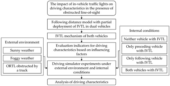
Figure 1.
The research flow chart of the paper.
2. Methods
2.1. Following Distance Model with Partial Deployment of IVTLs
In this study, due to the following distance during the straight-ahead phase of ORTLs being most evident, this phase was mainly considered. At the same time, considering the complexity and uncertainty of the reaction time and road conditions on driving characteristics, the reaction time and road conditions were not considered in the vehicle models. Simplification and focus on the study make the models easier to understand and explain. The proposed vehicle models present different deployment conditions of IVTLs, including one model where only the preceding vehicle is equipped with IVTLs, and a second model where only the following vehicle is equipped with IVTLs.
2.1.1. Only the Preceding Vehicle Equipped with IVTLs
The schematic diagram (Figure 2) illustrates the deployment condition in which only the preceding vehicle is equipped with IVTLs, and ORTL conditions include the display of both a green light and a red light. It is evident that the utilization of IVTLs extends the distance over which drivers can perceive (signal phase and timing message) SPAT, thereby influencing driving characteristics.
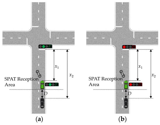
Figure 2.
The deployment condition of only the preceding vehicle equipped with IVTLs: (a) green light of ORTL; (b) red light of ORTL.
The driving status of only the preceding vehicle equipped with IVTLs is restricted by ORTLs. According to the status of ORTLs, both vehicles exhibit the corresponding driving status, as shown in Figure 3.
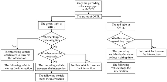
Figure 3.
Driving status of both vehicles under only the preceding vehicle equipped with IVTLs.
Green Light of ORTL
The illustration in Figure 4 portrays the displacement curve of the vehicle strategies in the scenario of a green light indication from the ORTL. The vehicle strategies depict the operational state of the vehicles under standard driving conditions, specifically, acceleration during the green traffic light indication and deceleration during the red traffic light indication.
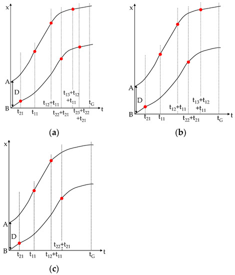
Figure 4.
The displacement curve of the preceding vehicle equipped with IVTLs during a green light indication from ORTLs and including three scenarios: (a) both vehicles traverse the intersection; (b) only the preceding vehicle traverses the intersection; (c) neither the preceding vehicle nor the following vehicle traverses the intersection.
Only the preceding vehicle is equipped with IVTLs, which can obtain SPAT information from a farther distance than the following vehicle. When the ORTL is displayed as green, compared with the case without IVTL deployment, the preceding vehicle can accelerate appropriately to pass the intersection faster and arrive at the intersection within the remaining time of the green light. The following vehicle can also accelerate correspondingly, but the pass-ability of the preceding vehicle is greater than that of the following vehicle. Therefore, on the green traffic light indication, there are three possible scenarios for the traversal of the intersection by the two vehicles, namely, both vehicles traversing the intersection, only the preceding vehicle traversing the intersection, and neither the preceding vehicle nor the following vehicle traversing the intersection. These three scenarios correspond to the ORTL being green with longer remaining time, the ORTL being green with shorter remaining time, and the ORTL beginning to turn yellow or red with longer remaining time, respectively. A detailed analysis of each of these scenarios is provided below.
- Both vehicles traverse the intersection
If the distance between the preceding vehicle and the stop line, denoted as x1, is less than the maximum distance, denoted as xG, that the vehicle can travel within the remaining green time, denoted as tG, the vehicle will be able to traverse the intersection. As depicted in Figure 4a, the preceding vehicle initiates acceleration with a′11 and reaches the road speed limit vRSL within time t11. The vehicle then maintains this speed for the duration of time t12. Then, as the vehicle approaches the intersection, it reduces speed to the intersection speed limit vISL over a period of time t13, until traversing the intersection. The maximum distance xG1 that the vehicle can travel within the remaining green time tG can be calculated using Equation (1). The following vehicle initially maintains its initial speed v2 for a duration of time t21, subsequently increasing its speed to v′2 (which is less than vRSL) over time t22. The trajectory of this vehicle is similar to that of the preceding vehicle, as described by Equation (2), whereby the maximum distance xG2 that the vehicle can travel within the remaining green time tG can be calculated. The distance covered by the following vehicle over time can be computed using Equation (3).
- Only the preceding vehicle traverses the intersection
In the vehicle strategy where only the preceding vehicle traverses the intersection, the following vehicle reduces its speed until it comes to a stop at the stop line. The distance between the following vehicle and the stop line, denoted as x2, is greater than the maximum distance, denoted as xG2, that the vehicle can travel within the remaining green time, denoted as tG, which can be calculated using Equation (4).
In this scenario, the distance covered by the following vehicle over time, denoted as D′, can be computed using Equation (5).
- Neither the preceding vehicle nor the following vehicle traverses the intersection
In the event that both vehicles are unable to traverse the intersection, as depicted in Figure 4c, the maximum distances, xG1 and xG2, that each vehicle can travel within the remaining green time tG can be calculated using Equations (6) and (7), respectively.
As inferred from the displacement curve, the distance covered by the following vehicle over time, denoted as D′, can be calculated using Equation (8).
Red Light of ORTL
The displacement curve of the vehicle strategies in the scenario of a red light indication from the ORTL is illustrated in Figure 5. When the ORTL is displayed as red, compared with the case without IVTL deployment, the preceding vehicle can decelerate appropriately to pass through the intersection without stopping and arrive at the intersection outside the remaining time of the red light. The following vehicle is restricted by the state of the preceding vehicle and can only adopt deceleration measures. Therefore, on the red traffic light indication, there are two possible scenarios for the traversal of the intersection by the two vehicles, namely, both vehicles traversing the intersection and neither the preceding vehicle nor the following vehicle traversing the intersection. These two scenarios correspond to the ORTL being red with shorter remaining time (the ORTL beginning to turn green with longer remaining time), and the ORTL being yellow or red with longer remaining time.
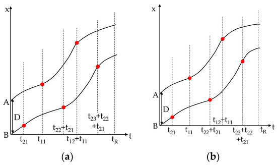
Figure 5.
The displacement curve of the preceding vehicle equipped with IVTLs during a red light indication from the ORTL and including two scenarios: (a) both vehicles traverse the intersection; (b) neither the preceding vehicle nor following vehicle traverses the intersection.
- Both vehicles traverse the intersection
In the vehicle strategy where both vehicles traverse the intersection, if the distance between the preceding vehicle and the stop line, denoted as x1, is less than the maximum distance, denoted as xR, that the vehicle can travel within the remaining time, denoted as tR, the vehicle will be unable to traverse the intersection. The maximum distances, xR1 and xR2, that the preceding and following vehicles can travel within the remaining time tR, respectively, can be determined by applying Equations (9) and (10). As illustrated in Figure 5a, the preceding vehicle, by decelerating at a rate of a11, reduces its velocity to v′1 over the course of time t11, while the following vehicle maintains its initial velocity for a duration of time t21. Subsequently, the preceding vehicle, by accelerating at a rate of a′11, increases its velocity to v″1 over time t12. Furthermore, the following vehicle, by first decelerating at a rate of a21 and then accelerating at a rate of a′21, over time t22 and t23, respectively, adjusts its velocity. Finally, both the preceding and following vehicles reduce their velocities below the intersection speed limit to traverse the intersection.
The distance-over-time of the following vehicle can be obtained by applying Equation (11).
- Neither the preceding vehicle nor following vehicle traverses the intersection
In this vehicle strategy, the preceding vehicle decelerates until it comes to a stop at the stop line. The maximum distances, xR1 and xR2, that the preceding and following vehicles can travel within the remaining time tR can be determined by applying Equations (12) and (13), respectively. Furthermore, the distance-over-time of the following vehicle, D′, can also be obtained by utilizing Equation (11).
2.1.2. Only the Following Vehicle Equipped with IVTLs
The scenario in which only the following vehicle is equipped with IVTLs is depicted in Figure 6. The conditions of the green and red traffic lights are illustrated in Figure 6a,b, respectively.
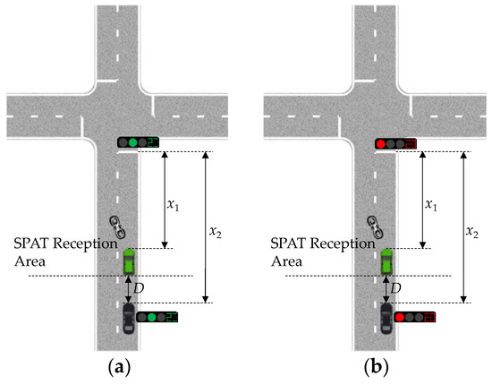
Figure 6.
The deployment condition of only the following vehicle equipped with IVTLs: (a) green light of the ORTL; (b) red light of the ORTL.
The driving status of only the following vehicle equipped with IVTLs is restricted by ORTLs and the driving status of the preceding vehicle. According to the status of ORTLs and the preceding vehicle, both vehicles exhibit corresponding driving status, as shown in Figure 7.
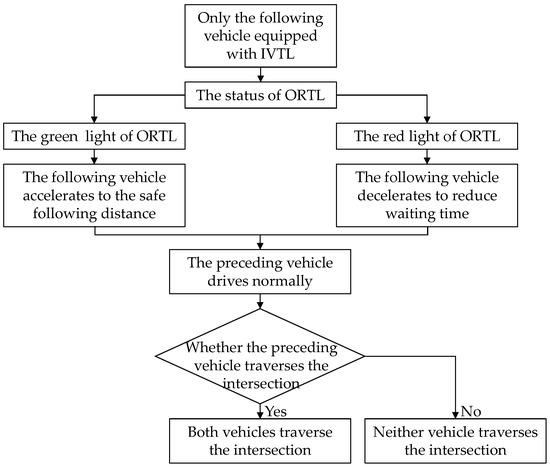
Figure 7.
Driving status of both vehicles under only the following vehicle equipped with IVTLs.
Green Light of ORTLs
The trajectory of the vehicles in the green light scenario, where only the following vehicle is equipped with IVTLs, is illustrated in Figure 8. Only the following vehicle is equipped with IVTLs, which can obtain SPAT information from a farther distance than the preceding vehicle. When the ORTL is displayed as green, compared with the case without IVTL deployment, the following vehicle can accelerate to the safe following distance. The preceding vehicle cannot obtain SPAT remotely, which is in the normal driving state. Whether the following vehicle can traverse the intersection depends entirely on the preceding vehicle. Therefore, on the green traffic light indication, there are two possible scenarios for the traversal of the intersection by the two vehicles, namely, both vehicles traversing the intersection, and neither the preceding vehicle nor the following vehicle traversing the intersection.
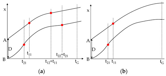
Figure 8.
The displacement curve of the following vehicle equipped with IVTLs during a green light indication from the ORTL and including two scenarios: (a) both vehicles traverse the intersection; (b) neither the preceding vehicle nor following vehicle traverses the intersection.
- Both vehicles traverse the intersection
As shown in Figure 8a, the preceding vehicle strategy is similar to the vehicle that is not equipped with IVTLs. First, the initial velocity in time t11 is maintained and then decreased to the intersection speed limit in time t12, and the velocity is maintained in time t13. However, the following vehicle with acceleration a′21 increases the velocity to v′2 (below vRSL) in time t21, and then with deceleration a21 decreases to the intersection speed limit using time t22. Finally, the vehicle retains the velocity in time t23. In addition, xG1 and xG2 can be calculated by Equations (14) and (15), respectively.
Combined with the displacement curve, the following distance over time D′ can be calculated by Equation (16).
- Neither the preceding vehicle nor following vehicle traverses the intersection
If the preceding vehicle cannot cross the intersection, the following vehicle also can-not cross the intersection. The displacement curve is shown in Figure 8b. xG1 and xG2 can easily be obtained using Equations (17) and (18), respectively.
Subsequently, the temporal distance metric, D′, can be calculated utilizing Equation (19).
Red Light of the ORTL
The displacement curve of the scenario of the red traffic light with only the following vehicle equipped with IVTLs is depicted in Figure 9. When the ORTL is displayed as yellow or red, compared with the case without IVTL deployment, the following vehicle can decelerate to reduce waiting time for stopping. The preceding vehicle can still drive normally. Whether the following vehicle can traverse the intersection depends entirely on the preceding vehicle. Therefore, on the red traffic light indication, there are two possible scenarios for the traversal of the intersection by the two vehicles, namely, both vehicles traversing the intersection, and neither the preceding vehicle nor the following vehicle traversing the intersection.
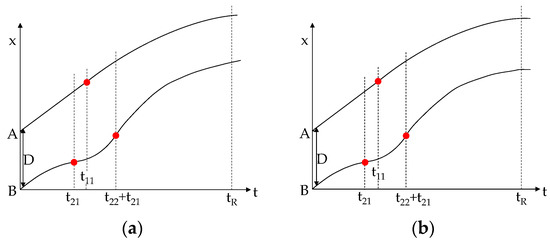
Figure 9.
The displacement curve of only the following vehicle equipped with IVTLs during a red light indication from the ORTL and including two scenarios: (a) both vehicles traverse the intersection; (b) neither the preceding vehicle nor following vehicle traverses the intersection.
- Both vehicles traverse the intersection
For the successful traversal of the intersection by both vehicles, it is essential that the distance between the preceding vehicle and the stop line, denoted as x1, exceeds the maximum distance that the vehicle can cover in the remaining time, tR, represented as xR1. Analogously, the same condition applies to the subsequent vehicle. The values of xR1 and xR2 can be computed through the application of Equations (20) and (21), respectively. As depicted in Figure 9a, during the latter stages of the journey, the preceding vehicle reduces its speed as opposed to coming to a complete halt at the stop line. This is achieved through a combination of deceleration, denoted as a21, which reduces the velocity to v′2 in time t21, followed by acceleration, denoted as a′21, which increases the velocity to v″2 (below vRSL) in time t22, and finally deceleration, denoted as a22, which reduces the velocity to v‴2 in time t23.
In the latter scenario, the temporal distance metric, D′, can be determined by utilizing Equation (22).
- Neither the preceding vehicle nor following vehicle traverses the intersection
In the event that the intersection cannot be traversed by both the preceding and following vehicles, the vehicle strategy is illustrated in Figure 9b. The maximum distance that the preceding vehicle can travel in the remaining time, tR, denoted as xR1, and the same for the following vehicle, denoted as xR2, can be computed through the application of Equations (23) and (24), respectively. Furthermore, the temporal distance metric, D′, can also be obtained through the utilization of Equation (22).
2.1.3. IVTL Mechanism of Both Vehicles
Vehicles equipped with IVTLs can receive SPAT, and their drivers can slow down or speed up in advance based on the status of the ORTL, thereby reducing waiting time and intersection congestion. When only the preceding vehicle is equipped with IVTLs, it will try to drive to the nearest position to the intersection stop line before the ORTL turns red and then wait for the green light. At the same time, the following vehicle without IVTLs can adjust its own driving status according to the driving status of preceding vehicle, ensuring a safe following distance. When the preceding vehicle speeds up, the following vehicle will also speed up, and when the preceding vehicle slows down, the following vehicle will also slow down. When only the following vehicle is equipped with IVTLs, its driving status is limited by the driving status of the preceding vehicle, but the following vehicle can also approach the preceding vehicle as much as possible while ensuring safety through acceleration and deceleration strategies. Currently, only a part of the vehicles is equipped with IVTLs, so the proposed two-vehicle following distance model does not include all situations. However, this model shows that the IVTL mechanism for two vehicles needs to consider factors such as relative vehicle speed, acceleration and deceleration, and following distance between the two vehicles to ensure safe driving and smooth traffic flow.
2.2. Evaluation Indicators
In the above-mentioned model for the following distance between two vehicles, the IVTL is introduced to extend the reception range of SPAT, thereby increasing the possible passing strategies. However, this also leads to closer vehicle interactions, and the model emphasizes the importance of the following distance. From the model, it can be seen that the maximum distance that can be traveled within the remaining time of the ORTL is related to driving maneuverability. Therefore, the travel time is chosen as an evaluation indicator for driving maneuverability. By using Equation (25), the average travel time of the preceding and following vehicles can be obtained.
wherein Tpreceding denotes the travel time of the preceding vehicle, and Tfollowing denotes the travel time of the subsequent vehicle. The metric Taverage signifies the average travel time of both the preceding and following vehicles.
As time changes, the following distance will be affected by various factors, including vehicle speed, acceleration, deceleration, travel time, etc. The following distance can also be used as an indicator to evaluate driving safety. In addition, TTC is also one of the indicators to evaluate driving safety, which is calculated by the following distance and relative speed. When 0 < TTC < the minimum time to conflict (minTTC), the following distance is considered too close, and there is a risk of collision, which is unsafe. On the contrary, when TTC > minTTC, it is a safe state, and the larger the value, the higher the safety, so minTTC can also be used as an evaluation indicator of driving safety. TTC can be calculated by the following formula:
wherein Vfollowing denotes the velocity of the subsequent vehicle, Vpreceding denotes the velocity of the preceding vehicle, and D represents the following distance.
With respect to vehicle comfort, the maximum rates of change in the absolute values of the steering angle (maxS) and brake pressure (maxP) are considered as crucial indicators. The rate of change in the absolute value of the steering angle serves as an indicator of the driver’s stability while executing a turn and can be computed through the following equation:
where S′ denotes the rate of change in the absolute value of the steering angle, St represents the absolute value of the steering angle at a given instant, St+nT represents the absolute value of the steering angle at the subsequent instant, and T signifies the sampling period.
The rate of change in the absolute value of the brake pressure serves as an indicator of the speed at which the driver depresses or releases the brake pedal, thereby characterizing the smoothness and stability of the driving experience. The equation for this metric is presented in Equation (28).
wherein P′ denotes the rate of change in the absolute value of the brake pressure, Pt represents the absolute value of the brake pressure at a given instant, and Pt+nT represents the absolute value of the brake pressure at the subsequent instant.
2.3. Simulated Scenarios with Obstructed ORTLs
Compared to V2X on actual roads, communication between vehicles and road in-frastructure is easier to achieve in simulation software of PreScan 8.5 and MATLAB/Simulink R2018b. Based on existing modules, simulation software can achieve the same effect as actual road V2X, which lays a solid foundation for later driving simulation experiments. In simulation software, settings need to be made for both the “vehicle” and “road” sides.
2.3.1. “Vehicle” Configuration of Simulation Software
In actual V2X scenarios, the vehicle side not only needs to have installed high-precision onboard sensors to obtain road condition information, but it also needs to collect road information sent by the roadside unit through the onboard unit and then display it in the onboard system to achieve environmental perception and long-distance warning functions. The PreScan simulation software can comprehensively develop and test advanced driver assistance systems, including sensor models, scene generation functions, vehicle dynamics options, third-party software and hardware interfaces, etc. The software has a clear and simple graphical user interface, and it provides multiple sensors and visual pedestrian and vehicle models. The main control module is based on MATLAB/Simulink software, which can directly call the functions of Simulink. In the simulation software, the “vehicle” side needs to have installed a traffic participant information receiver to detect the distance from the preceding vehicle and a radiofrequency onboard unit for short-distance communication. At the same time, the simulation vehicle is set to a two-dimensional vehicle dynamics model, and the Logitech G29 controller and automatic transmission are selected. Finally, the vehicle’s position information (horizontal and vertical coordinates), speed, throttle opening, steering wheel angle, and brake pedal pressure are output to the workspace of MATLAB simulation software.
For the “vehicle” side, a human–machine interface also needs to be set up, which requires real-time display of the current vehicle speed and the SPAT of ORTLs within the SPAT receiving range. To achieve the human–machine interface, the application modules in MATLAB can be used. Firstly, sub-modules are dragged from the component library to the design panel generating the target interface, then the view is switched to the code view, adding the corresponding code and initialization function, and finally the ORTL phase and timing in Simulink are configured.
2.3.2. “Road” Configuration of Simulation Software
In V2X on actual roads, in addition to upgrading and transforming detection equipment into intelligent connected devices, the roadside unit must also be connected to promptly issue warning information, SPAT, and traffic flow status to the onboard unit. In simulation software, the setting of simulation scenarios is classified as “road” side settings, including scenarios such as sunny, foggy, and ORTLs obstructed by a large vehicle, as well as different deployments of IVTLs if two vehicles are considered. The overview of the simulation scenarios is shown in Table 1. In addition, the “road” side also needs to set up ORTLs with a timing plan of 33 s for red lights, 30 s for green lights, and 3 s for yellow lights, only considering the straight-through phase. It is also equipped with radiofrequency beacons that communicate wirelessly with the radiofrequency onboard unit on the “vehicle” side to achieve unobstructed communication when receiving SPAT within a specified range.

Table 1.
Experimental conditions.
3. Experiment
3.1. Participants
The recruitment information for the experiment was disseminated through public announcements within the school. During the recruitment process, participants were provided with a brief overview of the experimental content and the minimal risk of simulator sickness. Additionally, the participants were ensured that they had no connection to the research team. Following confirmation, on the first day of the experiment, participants were familiarized with the experimental equipment and procedures, and the formal experiments were conducted on the second day. In total, 50 participant drivers were recruited for the study comprised of 25 males and 25 females, none of whom were professional drivers. The age range of the participants was between 20 and 40 years old, with a mean age of 30.2 years. All participants held a valid driving license, with a mean acquisition period of 5.9 years. All participants had visual acuity (including corrected visual acuity) of above 1.0 in both eyes. The participants were in good physical condition and exhibited high energy levels during the test.
3.2. Experimental Apparatus
In the experiment, two sets of Logitech G29 driving simulation equipment, a notebook computer, and two 17-inch displays were employed. Figure 10 depicts the visual representation of two test subjects operating the driving simulators.
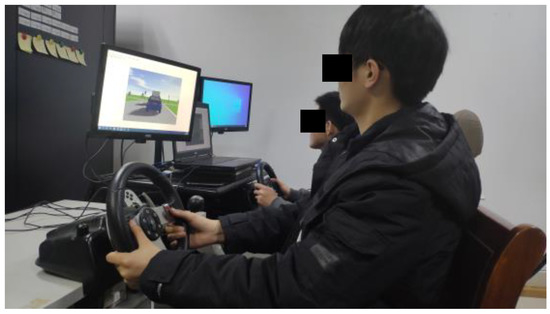
Figure 10.
The visual representation of two test subjects operating driving simulation equipment.
3.3. Experiment Process
The experimental setup, as illustrated in Figure 11, encompassed crucial information such as the driving route, static elements present, and the range of reception of the IVTL. To ensure that the participants were adequately acclimated to the operation of the driving simulators, additional routes were implemented in addition to the primary driving route. Adequate time was allocated prior to the commencement of the test, allowing participants to familiarize themselves with the driving simulators and the driving route.
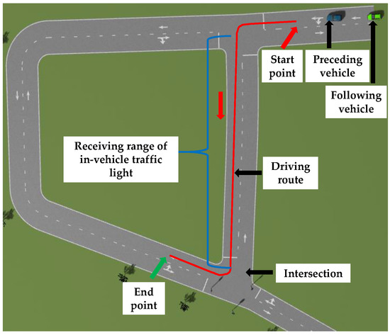
Figure 11.
The fundamental details of the experiment.
As depicted in Table 1, the experimental design included various scenarios of line-of-sight obstruction to ORTLs and different deployment conditions of IVTLs. Specifically, three scenarios of ORTL obstruction were considered, including sunny weather, foggy weather, and a truck obstructing the ORTLs. Additionally, different deployment conditions of IVTLs were evaluated, including both vehicles being equipped with IVTLs, only the preceding vehicle being equipped with IVTLs, only the following vehicle being equipped with IVTLs, and both vehicles being unequipped with IVTLs. The control group for the experiments consisted of sunny weather and both vehicles being unequipped with IVTLs, while the experimental groups included foggy weather, ORTL obstruction by a truck, and various deployment conditions of IVTLs. The results were then compared across the different scenarios and deployment conditions to assess the influence of IVTLs on driving characteristics under line-of-sight obstruction to the ORTLs.
The subject pool of fifty participants was systematically divided into twenty-five pairs through a randomized process. Each dyad consisted of one individual operating the virtual leading vehicle and the other operating the virtual trailing vehicle. The experiment was executed with a counterbalanced design, with data outputted including metrics such as speed, location, steering angle, throttle opening, brake pressure, and the following distance of both the leading and trailing virtual vehicles. Illustrative screenshots of the scenarios are presented in Figure 12.
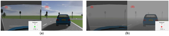
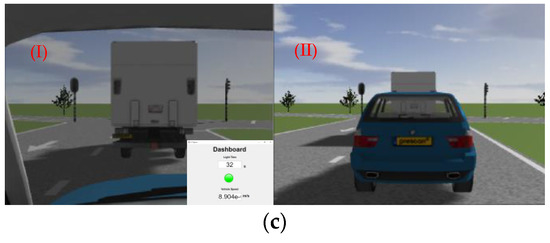
Figure 12.
Illustrative visualizations of the simulated scenarios: (a) natural driving conditions with the preceding vehicle equipped with IVTLs; (b) foggy environment with the following vehicle equipped with IVTL; (c) the ORTLs blocked by a truck with the preceding vehicle equipped with IVTLs. (I) The perspective of the preceding vehicle; (II) the perspective of the following vehicle.
4. Analysis
The data of vehicle status were sampled at a frequency of 20 Hz. After completing the driving simulator experiment, the data of vehicle status were directly obtained from the simulation software. Then, the data were filtered and transformed to the evaluation indicators of driving characteristics. To highlight the differences between evaluation indicators, minTTC, Taverage, maxS and maxP were extracted. Finally, the evaluation indicators were classified according to the scenarios and different deployments of IVTLs. The statistical significance threshold was set at 0.05. External environmental factors (sunny or foggy weather or ORTLs obstructed by a large vehicle) and internal conditions (incomplete or complete deployment of IVTLs) were used as variables for one-way analysis of variance.
4.1. Analysis of Driving Safety
This study used minTTC as the primary indicator to evaluate driving safety. Figure 13 shows the distribution of minTTC under the influence of the external environment and internal conditions. The numerical values marked with a red “+” sign are considered outliers for this data. Due to their extremely high or low values, they may have an impact on the overall analysis. Therefore, they have been removed from the dataset.
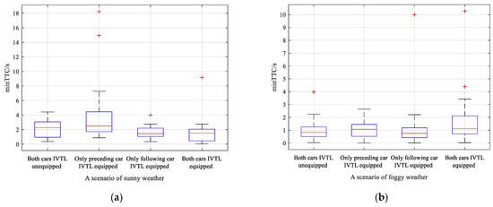
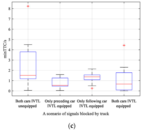
Figure 13.
Outcome of minTTC derived from the designed external environment and internal conditions: (a) outcome of minTTC in the scenario of sunny weather; (b) outcome of minTTC in the scenario of foggy weather; (c) outcome of minTTC in the scenario of being blocked by a truck.
A one-way analysis of variance was performed focusing on the impact of different internal conditions under the same external environment. In sunny and foggy scenarios, the indicator did not meet the homogeneity of variance condition (p = 0.053 > 0.05, p = 0.399 > 0.05), but in the scenario of ORTLs obstructed by a large vehicle, the indicator met the homogeneity of variance condition (p = 0.020 < 0.05). In this scenario, compared to the non-deployment of IVTLs, minTTC was reduced by about 50% (p = 0.019 < 0.05), indicating that the deployment of IVTLs in this scenario can effectively improve driving safety.
4.2. Analysis of Driving Maneuverability
The main evaluation indicator of driving maneuverability was travel time. Figure 14 shows the distribution of travel time under the influence of the external environment and internal conditions. Since the experiment started from the preceding vehicle entering the driving route and stopped when the following vehicle passed through the intersection and stopped, the travel time of the following vehicle was the same as Taverage. The numerical values marked with a red “+” sign are considered outliers for this data. Due to their extremely high or low values, they may have an impact on the overall analysis. Therefore, they have been removed from the dataset.
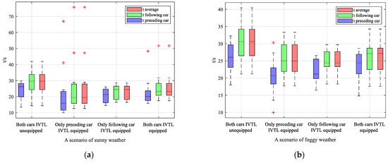
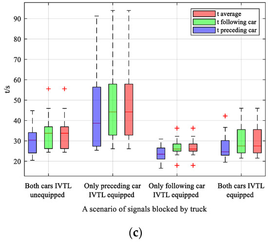
Figure 14.
Outcome of travel time from the designed external environment and internal conditions: (a) outcome of travel time in the scenario of sunny weather; (b) outcome of travel time in the scenario of foggy weather; (c) outcome of travel time in the scenario of being blocked a truck.
Similarly, a one-way analysis of variance was conducted on indicators with the same external environment and different internal conditions. In the foggy scenario, whether partially or fully equipped with IVTLs, the travel time of the preceding and following vehicles showed statistical significance (p = 0.018 < 0.05, p = 0.033 < 0.05). Specifically, in the foggy scenario, compared to the non-deployment of IVTLs, the travel time of the preceding and following vehicles was reduced (p = 0.017 < 0.05, p = 0.033 < 0.05). Taverage decreased by about 30%, indicating that deploying IVTLs can effectively improve driving maneuverability in this scenario.
4.3. Analysis of Driving Comfort
The main evaluation indicators for driving comfort were maxS and maxP, as shown in Figure 15 and Figure 16, respectively. The numerical values marked with a red “+” sign are considered outliers for this data. Due to their extremely high or low values, they may have an impact on the overall analysis. Therefore, they have been removed from the dataset.
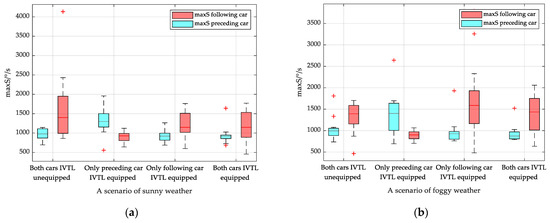
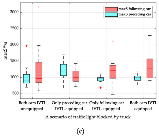
Figure 15.
Outcome of maxS from the designed external environment and internal conditions: (a) outcome of maxS in the scenario of sunny weather; (b) outcome of maxS in the scenario of foggy weather; (c) outcome of maxS in the scenario of being blocked by a truck.
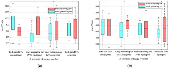
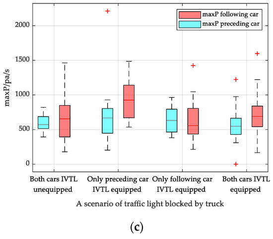
Figure 16.
Outcome of maxP from the designed external environment and internal conditions: (a) outcome of maxP in the scenario of sunny weather; (b) outcome of maxP in the scenario of foggy weather; (c) outcome of maxP in the scenario of being blocked by truck.
A one-way analysis of variance was performed focusing on the changes in the indicators under the same external environment but different internal conditions. In the sunny scenario, there were statistically significant differences in maxS of both vehicles (p = 0.000 < 0.05, p = 0.008 < 0.05). Specifically, compared to the non-deployment of IVTLs, the maxS of both vehicles decreased (p = 0.008 < 0.05, p = 0.023 < 0.05), with a decrease of about 15%. There were also statistically significant differences in maxP of both vehicles (p = 0.006 < 0.05, p = 0.033 < 0.05). Specifically, compared to the non-deployment of IVTLs, the maxS of both vehicles significantly decreased (p = 0.046 < 0.05, p = 0.001 < 0.05), with a decrease of about 10%. These indicated that deploying IVTLs in this scenario can effectively improve driving comfort.
5. Discussion
The IVTL system represents a pivotal technology in the realm of vehicle–road collaboration and serves to materialize the SPAT of ORTLs. Its in-vehicle display enables the driver to receive relevant information even in cases when the ORTLs are not discernible. Previous research has revealed that the integration of the IVTL system into the traffic flow results in a marked improvement, with flow rates being increased by over 60% and a significant reduction in carbon dioxide emissions, estimated at 18%. However, it must be acknowledged that the full integration of the IVTL system cannot be achieved in its entirety at present, thereby necessitating consideration of partial deployment scenarios. Research on the driving characteristics of IVTLs has mainly been conducted by Yang [25,27]. In [25], the capability of IVTLs in assisting drivers to navigate through unsignalized intersections was evaluated by a 100% penetration rate of IVTLs. The results showed that IVTLs significantly improved post-encroachment time and reduced the maximum brake stroke, thereby indicating an enhancement in driving safety. In [27], the impact of the IVTL system on driving conditions was evaluated by examining the interaction between IVTL-equipped and -unequipped vehicles as they exited an intersection. The results indicated that the deployment of IVTLs in the lead vehicle could significantly mitigate the maximum deceleration experienced by the trailing vehicle, even in cases where the latter was not equipped with the system. The present investigation, which outlines the road conditions and evaluation criteria, builds upon this previous research and further advances our understanding of the impact of IVTLs on driving conditions.
There has been a lack of theoretical analysis and specific explanation of the critical factors affecting driving characteristics under different deployment conditions of IVTLs. In addition, the experimental scenarios have been relatively limited without considering ORTL-obstructed scenarios. This study aimed to investigate the impact of line-of-sight obstructions to the ORTLs on driving characteristics and the efficacy of IVTLs in different deployment scenarios. Three distinct scenarios were considered: clear weather, inclement weather, and ORTLs obscured by an obstructing vehicle. A comprehensive set of evaluation metrics was proposed, including minTTC as a measure of vehicle safety, travel time as a measure of vehicle maneuverability, and maxS and maxP as indicators of vehicle comfort. Data were collected through two driving simulators using a sample of 50 participants. The results showed that under clear weather conditions, IVTL utilization improved vehicle comfort, reducing maxP of the preceding vehicle and maxS of the following vehicle. During inclement weather, IVTLs improved vehicle maneuverability by decreasing travel time and reduced the adverse effects of weather conditions on driver perception. In the scenario of ORTLs obscured by a truck, IVTLs improved vehicle safety, stabilizing driver’s speed and following distance and enhancing road efficiency, thereby avoiding the risk of running a red light.
Future studies ought to encompass the scenario of ORTLs obstructed by a truck, taking into account not only the characteristics of the truck but also the mechanisms of obstruction. To gain a more comprehensive understanding of the impact of IVTLs, it would be advantageous to incorporate physiological indicators of drivers into the evaluation process. Moreover, further research should explore the effectiveness of IVTLs in extreme weather conditions, such as heavy rain or snow, in scenarios where line-of-sight obstruction is caused by adverse weather environments. Ultimately, the optimization of IVTL placement and the improvement of display methods to provide a more intuitive head-up-display system would be intriguing avenues of study aimed at achieving the same level of efficacy with minimal driver distraction.
6. Conclusions
This study aimed to investigate the impact of IVTLs on driving characteristics, with a specific focus on line-of-sight obstruction to the ORTLs. To this end, three scenarios were considered, comprised of sunny weather, foggy weather, and ORTLs obstructed by a truck, in addition to different deployment of IVTLs between two vehicles. An analysis of driving characteristics under line-of-sight obstruction to ORTLs and IVTLs was conducted by selecting various vehicle models, driving safety, and maneuverability and comfort indicators. The relevant data were procured from driving simulators, and the aforementioned indicators were subsequently analyzed mathematically. The outcome of the study indicated an improvement in driving characteristics due to the implementation of IVTLs in scenarios of line-of-sight obstruction to ORTLs, which can be utilized as a case study for replication.
(1) With the objective of addressing the issue of line-of-sight obstruction to ORTLs at intersections, an IVTL system was proposed for signalized intersections. The system makes use of a SPAT message, containing information about the traffic light, which is transmitted to a vehicle equipped with the system within the range of reception. This assists the driver in navigating the intersection by providing real-time information about the traffic light status. The functionality of the system, including the transmission of traffic light information and the display of the human–machine interaction interface, was evaluated through the use of simulation software of PreScan 8.5 and MATLAB/Simulink R2018b.
(2) Three distinct scenarios of line-of-sight obstruction to the ORTLs were constructed utilizing the PreScan and Simulink software, and two varying scenarios of deployment of the IVTLs for two vehicles were employed. Additionally, corresponding vehicle models and targeted evaluation indicators were proposed. Evaluation indicators of vehicle safety, including minTTC, vehicle maneuverability corresponding to travel time, as well as vehicle comfort corresponding to maxS and maxP were analyzed to determine the driving characteristics.
(3) A comprehensive experiment was conducted to evaluate the impact of the IVTLs on driving characteristics utilizing a sample of 50 participants. The evaluation indicators, which were tailored to vehicle safety, maneuverability, and comfort, were analyzed based on one-way analyses of variance. The results indicated that in scenarios of sunny weather, the maxS and maxP were reduced by approximately 15% and 10%, respectively, in comparison to the same scenario without IVTLs, thus improving vehicle comfort. In scenarios of foggy weather, the Taverage was approximately 30% lower in comparison to the same scenario without IVTLs, indicating an improvement in vehicle mobility. In scenarios where the ORTLs were blocked by a truck, the minTTC was approximately 50% lower in comparison to the same scenario without IVTLs, thus enhancing vehicle safety. In conclusion, the IVTLs can effectively aid drivers in traversing intersections, even under conditions of line-of-sight obstruction to ORTLs and incomplete deployment of IVTLs.
Author Contributions
The idea, design, and testing were spearheaded by the first author, Y.Z. All co-authors played significant roles. Q.X. was responsible for building scenarios; M.G. contributed to the testing of the recruited testers; Y.G. contributed to data processing. The first author prepared the manuscript, which was reviewed by all co-authors. All authors have read and agreed to the published version of the manuscript.
Funding
This research was supported by the Post-Doctoral Research Foundation of China (Grant No. 2020M681497) and the Youth Talent Cultivation Program of Jiangsu University.
Institutional Review Board Statement
The study was conducted in accordance with the Declaration of Helsinki and approved by the Institutional Review Board (or Ethics Committee) of Jiangsu University (10 November 2021).
Informed Consent Statement
Informed consent was obtained from all subjects involved in the study.
Data Availability Statement
Not applicable.
Conflicts of Interest
The authors declare no conflict of interest.
References
- Lu, H.; Chen, M.; Kuang, W. The Impacts of Abnormal Weather and Natural Disasters on Transport and Strategies for Enhancing Ability for Disaster Prevention and Mitigation. Transp. Policy 2020, 98, 2–9. [Google Scholar] [CrossRef]
- Xu, M.; Wang, H.; Chu, S. Traffic Simulation and Visual Verification in Smog. ACM Trans. Intell. Syst. Technol. 2018, 10, 1–17. [Google Scholar] [CrossRef]
- Reinolsmann, N.; Alhajyaseen, W.; Brijs, T. Sandstorm Animations on Rural Expressways: The Impact of Variable Message Sign Strategies on Driver Behavior in Low Visibility Conditions. Transp. Res. Part F Traffic Psychol. Behav. 2021, 78, 308–325. [Google Scholar] [CrossRef]
- Sun, Y.; Xu, J. Research on Drivers’ Behavior Characteristics of Expressway Straight Section under Moderate Rainfall. IOP Conf. Ser. Earth Environ. Sci. 2021, 634, 012134. [Google Scholar] [CrossRef]
- Bobermin, M.P.; Silva, M.M.; Ferreira, S. Driving Simulators to Evaluate Road Geometric Design Effects on Driver Behaviour: A Systematic Review. Accid. Anal. Prev. 2021, 150, 105923. [Google Scholar] [CrossRef]
- Mohammed, D.; Aldoski, Z.; Kattan, R. Geometrical Design Errors in Duhok Intersections by Driver Behavior. J. Univ. Babylon Eng. Sci. 2018, 26, 395–410. [Google Scholar]
- Yan, Y.; Dai, Y.; Li, X.; Tang, J.; Guo, Z. Driving Risk Assessment Using Driving Behavior Data under Continuous Tunnel Environment. Traffic Inj. Prev. 2019, 20, 807–812. [Google Scholar] [CrossRef]
- Zhang, G.; Chen, J.; Zhao, J. Safety Performance Evaluation of a Three-Leg Unsignalized Intersection Using Traffic Conflict Analysis. Math. Probl. Eng. 2017, 2017, 2948750. [Google Scholar] [CrossRef]
- Manchon, J.; Bueno, M.; Navarro, J. How the Initial Level of Trust in Automated Driving Impacts Drivers’ Behaviour and Early Trust Construction. Transp. Res. Part F Traffic Psychol. Behav. 2022, 86, 281–295. [Google Scholar] [CrossRef]
- Toledo, G.; Shiftan, Y. Can Feedback from In-Vehicle Data Records Improve Driver Behavior and Reduce Fuel Comsumption? Transp. Res. Part A Policy Pract. 2016, 94, 194–204. [Google Scholar] [CrossRef]
- Yang, Y.; Yan, J.; Guo, J.; Kuang, Y.J.; Yin, M.Y.; Wang, S.N.; Ma, C.Y. Driving Behavior Analysis of City Buses based on Real-Time GNSS Traces and Road Information. Sensors 2021, 21, 687. [Google Scholar] [CrossRef]
- Kim, B.; Baek, Y. Sensor-Based Extraction Approaches of In-Vehicle Information for Driver Behavior Analysis. Sensors 2020, 20, 5197. [Google Scholar] [CrossRef]
- Noble, A.M.; Dingus, T.A.; Doerzaph, Z.R. Influence of In-Vehicle Adaptive Stop Display on Driving Behavior and Safety. IEEE Trans. Intell. Transp. Syst. 2016, 17, 2767–2776. [Google Scholar] [CrossRef]
- Bao, S.; Wu, L.; Yu, B.; Sayer, J.R. An Examination of Teen drivers’ Car-Following Behavior under Naturalistic Driving Conditions: With and without an Advanced Driving Assistance System. Accid. Anal. Prev. 2020, 147, 105762. [Google Scholar] [CrossRef]
- Gouribhatla, R.; Pulugurtha, S.S. Drivers’ Behavior when Driving Vehicles with or without Advanced Driver Assistance Systems: A Driver Simulator based Study. Transp. Res. Interd. Persp. 2022, 13, 100545. [Google Scholar] [CrossRef]
- Voinea, G.D.; Postelnicu, C.C.; Duguleana, M.; Mogan, G.L.; Socianu, R. Driving Performance and Technology Acceptance Evaluation in Real Traffic of a Smartphone-Based Driver Assistance System. Int. J. Environ. Res. Public Health 2020, 17, 7098. [Google Scholar] [CrossRef]
- Liu, R.; Yan, X.D.; Ma, S.W.; Xue, Q.W. Eye Movement as a Function to Explore the Effects of Improved Signs Design and Audio Warning on Drivers’ Behavior at STOP-Sign-Controlled Grade Crossings. Accid. Anal. Prev. 2022, 172, 106693. [Google Scholar] [CrossRef]
- Orlovska, J.; Novakazi, F.; Lars-Ola, B.; Karlsson, M.; Wickman, C.; Soderberg, R. Effects of the Driving Context on the Usage of Automated Driver Assistence Systems (ADAS)-Naturalistic Driving Study for ADAS Evaluation. Transp. Res. Interd. Persp. 2020, 4, 100093. [Google Scholar]
- Petraki, V.; Ziakopoulos, A.; Yannis, G. Combined Impact of Road and Traffic Characteristic on Driver Behavior Using Smartphone Sensor Data. Accid. Anal. Prev. 2020, 144, 105657. [Google Scholar] [CrossRef]
- Pappalardo, G.; Caponetto, R.; Varrica, R.; Cafiso, S. Assessing the Operational Design Domain of Lane Support System for Automated Vehicles in Different Weather and Road Conditions. J. Traffic Transp. Eng. 2022, 9, 631–644. [Google Scholar] [CrossRef]
- Pappalardo, G.; Cafiso, S.; Graziano, A.D.; Severino, A. Decision Tree Method to Analyze the Performance of Lane Support Systems. Sustainability 2021, 13, 846. [Google Scholar] [CrossRef]
- Zolali, M.; Mirbaha, B.; Layegh, M.; Behnood, H.R. A Behavioral Model of Drivers’ Mean Speed Influenced by Weather Conditions, Road Geometry, and Driver Characteristics Using a Driving Simulator Study. Adv. Civ. Eng. 2021, 2021, 5542905. [Google Scholar] [CrossRef]
- Yao, Y.; Zhao, X.H.; Zhang, Y.L.; Chen, C.; Rong, J. Modeling of Individual Vehicle Safety and Fuel Consumption under Comprehensive External conditions. Transp. Res. Part D Transp. Environ. 2020, 79, 102224. [Google Scholar] [CrossRef]
- Tonguz, O.K. Biologically Inspired Solutions to Fundamental Transportation Problem. IEEE Commun. Mag. 2011, 11, 106–115. [Google Scholar] [CrossRef]
- Yang, B.; Zheng, R.; Shimono, K.; Kaizuka, T.; Nakano, K. Evaluation of the Effects of In-Vehicle Traffic Light on Driving Performances for Unsignalised Intersections. IET Intell. Transp. Syst. 2017, 11, 76–83. [Google Scholar] [CrossRef]
- Yang, B.; Zheng, R.; Kaizuka, T.; Nakano, K. Influences of Waiting Time on Driver Behaviors While Implementing In-Vehicle Traffic Light for Priority-Controlled Unsignalized Intersections. J. Adv. Transp. 2017, 2017, 7871561. [Google Scholar] [CrossRef]
- Yang, B.; Zheng, R.; Kaizuka, T. Analysis of Driver Behaviors while Using In-Vehicle Traffic Light with Partial Deployment of V2I Communication. In Proceedings of the 2018 IEEE Intelligent Vehicles Symposium (IV), Changshu, China, 26–30 June 2018; pp. 19–24. [Google Scholar]
- Yang, B.; Kaizuka, T.; Nakano, K. Drivers’ Trust Model while Using In-Vehicle Traffic Lights in a Partial Deployment Scenario. In Proceedings of the 2019 IEEE Intelligent Transportation Systems Conference (ITSC), Auckland, New Zealand, 27–30 October 2019; pp. 1588–1593. [Google Scholar]
- Ferreira, M.; Fernandes, M.; Conceição, H. Self-Organized Traffic Control. In Proceedings of the Seventh ACM International Workshop on Vehicular Internetworking, Chicago, IL, USA, 24 September 2010; Association for Computing Machinery: New York, NY, USA, 2010; pp. 85–90. [Google Scholar]
- Ferrreira, M.; Ore, P.M. On the Impact of Virtual Traffic Lights on Carbon Emissions Mitigation. IEEE Trans. Intell. Transp. Syst. 2012, 13, 284–295. [Google Scholar] [CrossRef]
- Yang, B.; Wang, Z.; Nakano, K. Effects of Penetration Rates on the Application of In-Vehicle Traffic Lights at Unsignalized Intersections. Traffic Inj. Prev. 2022, 23, 260–265. [Google Scholar] [CrossRef]


Disclaimer/Publisher’s Note: The statements, opinions and data contained in all publications are solely those of the individual author(s) and contributor(s) and not of MDPI and/or the editor(s). MDPI and/or the editor(s) disclaim responsibility for any injury to people or property resulting from any ideas, methods, instructions or products referred to in the content. |
© 2023 by the authors. Licensee MDPI, Basel, Switzerland. This article is an open access article distributed under the terms and conditions of the Creative Commons Attribution (CC BY) license (https://creativecommons.org/licenses/by/4.0/).