
Estimating Toll Road Travel Times Using Segment-Based Data Imputation


Abstract
:1. Introduction
2. Related Works
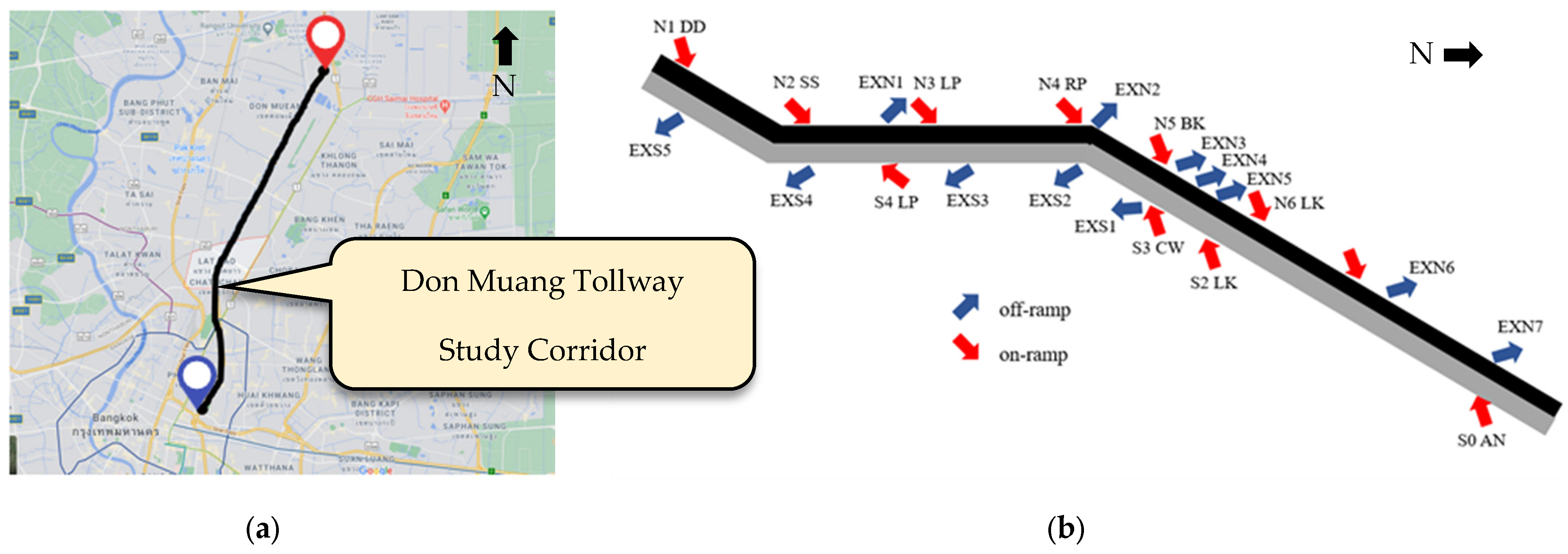
3. Study Corridor
3.1. Data Collection
3.2. Study Routes
4. Methodology
4.1. Data Cleaning and Imputation
4.2. Attribute Coding
4.3. Data Normalization
5. Model Development
5.1. Support Vector Regression
5.2. Recurrent Neural Networks
5.3. Model Performance Measurement
5.4. Hyperparameter Calibration and Optimization
6. Results
6.1. Effects of Data Imputation
6.2. Model Performance under Various Traffic Conditions
6.3. Model Performance under Unusual Traffic Conditions
- The inbound direction during the morning rush hour of 23 November 2020 (Monday), which was the first day of work following the long holiday, as shown in Figure 12.
- The outbound direction during the evening of 18 November 2020 (Wednesday), when people left the city for other provinces, as shown in Figure 13.
6.4. Effects of Missing Data on Model Performance
7. Discussion and Conclusions
Author Contributions
Funding
Institutional Review Board Statement
Informed Consent Statement
Data Availability Statement
Acknowledgments
Conflicts of Interest
References
- Liu, K.; Cui, M.-Y.; Cao, P.; Wang, J.-B. Iterative Bayesian Estimation of Travel Times on Urban Arterials: Fusing Loop Detector and Probe Vehicle Data. PLoS ONE 2016, 11, e0158123. [Google Scholar] [CrossRef] [PubMed]
- Peng, L.; Li, Z.; Wang, C.; Sarkodie-Gyan, T. Evaluation of Roadway Spatial-Temporal Travel Speed Estimation Using Mapped Low-Frequency AVL Probe Data. Measurement 2020, 165, 108150. [Google Scholar] [CrossRef]
- Haghani, A.; Hamedi, M.; Sadabadi, K.F.; Young, S.; Tarnoff, P. Data Collection of Freeway Travel Time Ground Truth with Bluetooth Sensors. Transp. Res. Rec. 2010, 2160, 60–68. [Google Scholar] [CrossRef]
- Sharifi, E.; Hamedi, M.; Haghani, A.; Sadrsadat, H. Analysis of Vehicle Detection Rate for Bluetooth Traffic Sensors: A Case Study in Maryland and Delaware. In Proceedings of the 18th World Congress on on Intelligent Transport Systems 2011, Orlando, FL, USA, 16–20 October 2011. [Google Scholar]
- Chen, M.; Xia, J.; Liu, R.R. Developing a Strategy for Imputing Missing Traffic Volume Data. J. Transp. Res. Forum 2010, 45, 57–75. [Google Scholar] [CrossRef]
- Liu, Y.; Xia, J.; Phatak, A. Evaluating the Accuracy of Bluetooth-Based Travel Time on Arterial Roads: A Case Study of Perth, Western Australia. J. Adv. Transp. 2020, 2020, 9541234. [Google Scholar] [CrossRef]
- Jedwanna, K.; Boonsiripant, S. Evaluation of Bluetooth Detectors in Travel Time Estimation. Sustainability 2022, 14, 4591. [Google Scholar] [CrossRef]
- Lipton, Z.C.; Kale, D.C.; Wetzel, R. Modeling Missing Data in Clinical Time Series with Rnns. Mach. Learn. Healthc. 2016, 56, 253–270. [Google Scholar]
- Xiangxue, W.; Lunhui, X.; Kaixun, C. Data-Driven Short-Term Forecasting for Urban Road Network Traffic Based on Data Processing and LSTM-RNN. Arab. J. Sci. Eng. 2019, 44, 3043–3060. [Google Scholar] [CrossRef]
- Chollet, F.; Allaire, J.J. Deep Learning Mit R Und Keras: Das Praxis-Handbuch von Den Entwicklern von Keras Und RStudio; MITP-Verlags GmbH & Co. KG: Frechen, Germany, 2018; ISBN 3958458955. [Google Scholar]
- Hearst, M.A.; Dumais, S.T.; Osuna, E.; Platt, J.; Scholkopf, B. Support Vector Machines. IEEE Intell. Syst. Their Appl. 1998, 13, 18–28. [Google Scholar] [CrossRef]
- Tan, H.; Wu, Y.; Cheng, B.; Wang, W.; Ran, B. Robust Missing Traffic Flow Imputation Considering Nonnegativity and Road Capacity. Math. Probl. Eng. 2014, 2014, 763469. [Google Scholar] [CrossRef]
- Qu, L.; Li, L.; Zhang, Y.; Hu, J. PPCA-Based Missing Data Imputation for Traffic Flow Volume: A Systematical Approach. IEEE Trans. Intell. Transp. Syst. 2009, 10, 512–522. [Google Scholar]
- Ni, D.; Leonard, J.D.; Guin, A.; Feng, C. Multiple Imputation Scheme for Overcoming the Missing Values and Variability Issues in ITS Data. J. Transp. Eng. 2005, 131, 931–938. [Google Scholar] [CrossRef]
- Luo, X.; Meng, X.; Gan, W.; Chen, Y. Traffic Data Imputation Algorithm Based on Improved Low-Rank Matrix Decomposition. J. Sens. 2019, 2019, 7092713. [Google Scholar] [CrossRef]
- Chen, J.; Shao, J. Nearest Neighbor Imputation for Survey Data. J. Off. Stat. 2000, 16, 113. [Google Scholar]
- Beretta, L.; Santaniello, A. Nearest Neighbor Imputation Algorithms: A Critical Evaluation. BMC Med. Inform. Decis. Mak. 2016, 16, 197–208. [Google Scholar] [CrossRef]
- Shin, D.-H.; Chung, K.; Park, R.C. Prediction of Traffic Congestion Based on LSTM through Correction of Missing Temporal and Spatial Data. IEEE Access 2020, 8, 150784–150796. [Google Scholar] [CrossRef]
- Tang, J.; Zou, Y.; Ash, J.; Zhang, S.; Liu, F.; Wang, Y. Travel Time Estimation Using Freeway Point Detector Data Based on Evolving Fuzzy Neural Inference System. PLoS ONE 2016, 11, e0147263. [Google Scholar] [CrossRef] [PubMed]
- Do, M.; Pueboobpaphan, R.; Miska, M.; Kuwahara, M.; van Arem, B. A Simple Data Fusion Method for Instantaneous Travel Time Estimation. In Proceedings of the 12th World Conference on Transport Research, Instituto Superior Tecnico (IST) 2010. Lisbon, Portugal, 11–15 July 2010; pp. 1–21. [Google Scholar]
- Li, R.; Rose, G.; Sarvi, M. Evaluation of Speed-Based Travel Time Estimation Models. J. Transp. Eng. 2006, 132, 540–547. [Google Scholar] [CrossRef]
- Xiao, Y.; Qom, S.F.; Hadi, M.; Al-Deek, H. Use of Data from Point Detectors and Automatic Vehicle Identification to Compare Instantaneous and Experienced Travel Times. Transp. Res. Rec. 2014, 2470, 95–104. [Google Scholar] [CrossRef]
- Kwon, J.; Coifman, B.; Bickel, P. Day-to-Day Travel-Time Trends and Travel-Time Prediction from Loop-Detector Data. Transp. Res. Rec. 2000, 1717, 120–129. [Google Scholar] [CrossRef]
- Zhang, M.; Wu, T.Q.; Kwon, E.; Sommers, K.; Habib, A. Arterial Link Travel Time Estimation Using Loop Detector Data; University of Iowa Public Policy Center: Iowa City, IA, USA, 1997; Volume 10, p. 2015. [Google Scholar]
- Samuel, A.L. Some Studies in Machine Learning Using the Game of Checkers. II—Recent Progress. IBM J. Res. Dev. 1967, 11, 601–617. [Google Scholar] [CrossRef]
- Bhavsar, P.; Safro, I.; Bouaynaya, N.; Polikar, R.; Dera, D. Machine Learning in Transportation Data Analytics. In Data Analytics for Intelligent Transportation Systems; Elsevier: Amsterdam, The Netherlands, 2017; pp. 283–307. [Google Scholar]
- Habtemichael, F.G.; Cetin, M. Short-Term Traffic Flow Rate Forecasting Based on Identifying Similar Traffic Patterns. Transp. Res. Part C Emerg. Technol. 2016, 66, 61–78. [Google Scholar]
- Yu, B.; Wang, H.; Shan, W.; Yao, B. Prediction of Bus Travel Time Using Random Forests Based on near Neighbors. Comput. Civ. Infrastruct. Eng. 2018, 33, 333–350. [Google Scholar] [CrossRef]
- Qiu, B.; Fan, W. Machine Learning Based Short-Term Travel Time Prediction: Numerical Results and Comparative Analyses. Sustainability 2021, 13, 7454. [Google Scholar] [CrossRef]
- Vanajakshi, L.; Rilett, L.R. Support Vector Machine Technique for the Short Term Prediction of Travel Time. In Proceedings of the 2007 IEEE Intelligent Vehicles Symposium, Istanbul, Turkey, 13–15 June 2007; IEEE: New York, NY, USA, 2007; pp. 600–605. [Google Scholar]
- Hou, Y.; Edara, P. Network Scale Travel Time Prediction Using Deep Learning. Transp. Res. Rec. 2018, 2672, 115–123. [Google Scholar] [CrossRef]
- Islek, I.; Oguducu, S.G. Use of LSTM for Short-Term and Long-Term Travel Time Prediction. In Proceedings of the CEUR Workshop Proceedings; the Creative Commons License Attribution 4.0 International; CEUR-WS: Aachen, Germany, 2019; Volume 2482. [Google Scholar]
- Liu, Y.; Wang, Y.; Yang, X.; Zhang, L. Short-Term Travel Time Prediction by Deep Learning: A Comparison of Different LSTM-DNN Models. In Proceedings of the 2017 IEEE 20th International Conference on Intelligent Transportation Systems (ITSC), Yokohama, Japan, 16–19 October 2017; IEEE: New York, NY, USA, 2017; pp. 1–8. [Google Scholar]
- Bai, C.; Peng, Z.-R.; Lu, Q.-C.; Sun, J. Dynamic Bus Travel Time Prediction Models on Road with Multiple Bus Routes. Comput. Intell. Neurosci. 2015, 2015, 432389. [Google Scholar] [CrossRef]
- Leys, C.; Ley, C.; Klein, O.; Bernard, P.; Licata, L. Detecting Outliers: Do Not Use Standard Deviation around the Mean, Use Absolute Deviation around the Median. J. Exp. Soc. Psychol. 2013, 49, 764–766. [Google Scholar] [CrossRef]
- Orr, J.M.; Sackett, P.R.; Dubois, C.L.Z. Outlier Detection and Treatment in I/O Psychology: A Survey of Researcher Beliefs and an Empirical Illustration. Pers. Psychol. 1991, 44, 473–486. [Google Scholar] [CrossRef]
- Li, L.; Li, Y.; Li, Z. Efficient Missing Data Imputing for Traffic Flow by Considering Temporal and Spatial Dependence. Transp. Res. Part C Emerg. Technol. 2013, 34, 108–120. [Google Scholar] [CrossRef]
- Cortes, C.; Vapnik, V. Support-Vector Networks. Mach. Learn. 1995, 20, 273–297. [Google Scholar]
- Gunn, S.R. Support Vector Machines for Classification and Regression. ISIS Tech. Rep. 1998, 14, 5–16. [Google Scholar]
- Wu, C.-H.; Ho, J.-M.; Lee, D.-T. Travel-Time Prediction with Support Vector Regression. IEEE Trans. Intell. Transp. Syst. 2004, 5, 276–281. [Google Scholar] [CrossRef]
- Liu, Y.; Ji, Y.; Chen, K.; Qi, X. Support Vector Regression for Bus Travel Time Prediction Using Wavelet Transform. J. Harbin Inst. Technol. (New Ser.) 2019, 26, 26–34. [Google Scholar]
- Graves, A. Long Short-Term Memory. In Supervised Sequence Labelling with Recurrent Neural Networks; Springer: Berlin/Heidelberg, Germany, 2012; pp. 37–45. [Google Scholar]
- Abbas, Z.; Al-Shishtawy, A.; Girdzijauskas, S.; Vlassov, V. Short-Term Traffic Prediction Using Long Short-Term Memory Neural Networks. In Proceedings of the 2018 IEEE International Congress on Big Data (BigData Congress), Seattle, WA, USA, 10–13 December 2018; IEEE: New York, NY, USA, 2018; pp. 57–65. [Google Scholar]
- Fu, R.; Zhang, Z.; Li, L. Using LSTM and GRU Neural Network Methods for Traffic Flow Prediction. In Proceedings of the 2016 31st Youth Academic Annual Conference of Chinese Association of Automation (YAC), Wuhan, China, 11–13 November 2016; IEEE: New York, NY, USA, 2016; pp. 324–328. [Google Scholar]
- Lewis, C.D. Industrial and Business Forecasting Methods: A Practical Guide to Exponential Smoothing and Curve Fitting; Butterworth-Heinemann: Oxford, UK, 1982; ISBN 0408005599. [Google Scholar]
- Thissen, U.; Van Brakel, R.; De Weijer, A.P.; Melssen, W.J.; Buydens, L.M.C. Using Support Vector Machines for Time Series Prediction. Chemom. Intell. Lab. Syst. 2003, 69, 35–49. [Google Scholar] [CrossRef]
- Cui, Z.; Ke, R.; Pu, Z.; Wang, Y. Stacked Bidirectional and Unidirectional LSTM Recurrent Neural Network for Forecasting Network-Wide Traffic State with Missing Values. Transp. Res. Part C Emerg. Technol. 2020, 118, 102674. [Google Scholar] [CrossRef]
- Zhang, H.; Wu, H.; Sun, W.; Zheng, B. Deeptravel: A Neural Network Based Travel Time Estimation Model with Auxiliary Supervision. arXiv Prepr. 2018, arXiv:1802.02147. [Google Scholar]
- Chen, D.; Yan, X.; Li, S.; Wang, L.; Liu, X. Long Short-Term Memory Neural Network for Travel Time Prediction of Expressways Using Toll Station Data. In Proceedings of the CICTP 2020, Xi’an, China, 14–16 August 2020; pp. 73–85. [Google Scholar]


| Route Code | Direction | Origin | Destination | Length (km) | No. of VIPSs | Mean Travel Time (min) | Standard Deviation of Travel Time (min) |
|---|---|---|---|---|---|---|---|
| OB_L | Outbound | Din Daeng | Anusorn Sathan | 19.1 | 68 | 12.01 | 1.99 |
| OB_S | Outbound | Din Daeng | Cheangwattana | 10.6 | 40 | 6.41 | 1.26 |
| IB_L | Inbound | Anusorn Sathan | Din Daeng | 18.9 | 70 | 12.21 | 2.13 |
| IB_S | Inbound | Anusorn Sathan | Lat Prao | 13.6 | 47 | 8.87 | 1.65 |
| Variables | Description | Variable Type | Example |
|---|---|---|---|
| AVGSPEED_ [CAMERAID] | Average speed (km/h) at 1 min intervals | Continuous | AVGSPEED_007, AVGSPEED_008, …, AVGSPEED_184 |
| TOTALCOUNTS_ [CAMERAID] | Vehicle count (veh/min) | Continuous | TOTALCOUNTS_ 007, TOTALCOUNTS_ 008 …, TOTALCOUNTS_184 |
| MISSDATAIND_ [CAMERAID] | Missing data indicator | Dummy | 1: Missing Data 0: Otherwise |
| DOW1 DOW2 DOW3 DOW4 DOW5 DOW6 | Day of week | Dummy | {DOW1 = 0, DOW2 = 0, …, DOW6 = 0} for Sunday; {DOW1 = 1, DOW2 = 0, …, DOW6 = 0} for Monday; {DOW1 = 0, DOW2 = 1, …, DOW6 = 0} for Tuesday; … |
| HR06 HR07 HR08 HR23 | Time of day | Dummy | {HR07 = 0, HR08 = 0, …, HR23 = 0} for 06:00–06:59; {HR07 = 1, HR08 = 0, …, HR23 = 0} for 07:00–07:59; {HR07 = 0, HR08 = 1, …, HR23 = 0} for 08:00–08:59; … |
| HOLIDAY | Holiday indicator | Dummy | HOLIDAY = 1 if holiday; HOLIDAY = 0 otherwise |
| B_HOLIDAY | Day-before-holiday indicator | Dummy | B_HOLIDAY = 1 if before the holiday; B_HOLIDAY = 0 otherwise |
| A_HOLIDAY | Day-after-holiday indicator | Dummy | A_HOLIDAY = 1 if after the holiday; A_HOLIDAY = 0 otherwise |
| Parameters | OB_L | OB_S | IB_L | IB_S |
|---|---|---|---|---|
| SVR | ||||
| 0.1 | 0.1 | 0.1 | 0.1 | |
| 10 | 1000 | 1000 | 1 | |
| 0.001 | 0.0001 | 0.0001 | 0.001 | |
| LSTM | ||||
| Learning rate | 0.01 | 0.01 | 0.01 | 0.01 |
| Batch size | 128 | 128 | 128 | 128 |
| Epoch | 45 | 20 | 65 | 65 |
| Route | Distance(km) | Period | MAPE (%) | MAE (min) | RMSE (min) | |||||||||
|---|---|---|---|---|---|---|---|---|---|---|---|---|---|---|
| IM | MLR | SVR | LSTM | IM | MLR | SVR | LSTM | IM | MLR | SVR | LSTM | |||
| IB_L | 18.9 | AM | 11.27 | 14.18 | 7.64 | 7.37 | 2.00 | 2.92 | 1.77 | 1.32 | 3.34 | 5.98 | 4.91 | 2.57 |
| MD | 3.14 | 2.92 | 3.42 | 2.97 | 0.37 | 0.34 | 0.39 | 0.34 | 0.47 | 0.43 | 0.50 | 0.43 | ||
| PM | 6.07 | 3.45 | 3.07 | 2.81 | 0.74 | 0.42 | 0.37 | 0.34 | 0.84 | 0.54 | 0.45 | 0.43 | ||
| ALL | 6.68 | 6.07 | 4.18 | 4.15 | 1.48 | 1.24 | 0.69 | 0.55 | 2.53 | 2.69 | 2.09 | 1.10 | ||
| IB_S | 13.6 | AM | 14.09 | 13.29 | 5.90 | 3.94 | 1.78 | 2.19 | 0.92 | 0.46 | 2.58 | 4.57 | 2.13 | 0.65 |
| MD | 5.77 | 4.08 | 3.01 | 2.76 | 0.50 | 0.35 | 0.26 | 0.24 | 0.57 | 0.43 | 0.33 | 0.29 | ||
| PM | 10.18 | 4.20 | 3.72 | 4.19 | 0.93 | 0.38 | 0.33 | 0.38 | 1.01 | 0.46 | 0.42 | 0.45 | ||
| ALL | 9.67 | 6.21 | 4.19 | 4.01 | 1.37 | 0.96 | 0.47 | 0.40 | 2.03 | 1.99 | 1.21 | 0.63 | ||
| OB_L | 19.1 | AM | 11.30 | 6.79 | 4.17 | 4.44 | 1.38 | 0.81 | 0.52 | 0.56 | 1.66 | 1.08 | 0.88 | 0.88 |
| MD | 9.36 | 5.68 | 3.60 | 3.50 | 1.11 | 0.67 | 0.42 | 0.41 | 1.22 | 0.83 | 0.53 | 0.52 | ||
| PM | 18.33 | 11.30 | 5.91 | 5.28 | 2.67 | 1.62 | 0.74 | 0.78 | 3.09 | 2.04 | 1.19 | 1.04 | ||
| ALL | 11.05 | 7.70 | 3.89 | 3.77 | 2.30 | 1.18 | 0.63 | 0.56 | 3.36 | 2.01 | 1.09 | 0.92 | ||
| OB_S | 10.6 | AM | 4.04 | 6.09 | 2.82 | 2.46 | 0.25 | 0.38 | 0.18 | 0.16 | 0.33 | 0.49 | 0.31 | 0.26 |
| MD | 2.86 | 5.27 | 1.99 | 2.28 | 0.18 | 0.33 | 0.12 | 0.14 | 0.22 | 0.41 | 0.15 | 0.17 | ||
| PM | 11.07 | 15.97 | 5.44 | 3.84 | 0.94 | 1.33 | 0.47 | 0.32 | 1.31 | 1.81 | 0.75 | 0.49 | ||
| ALL | 5.63 | 8.21 | 2.97 | 2.87 | 0.70 | 0.72 | 0.25 | 0.23 | 1.22 | 1.27 | 0.48 | 0.48 | ||
| Route | Period | MAPE (%) | MAE (min) | RMSE (min) | |||||||||
|---|---|---|---|---|---|---|---|---|---|---|---|---|---|
| IM | MLR | SVR | LSTM | IM | MLR | SVR | LSTM | IM | MLR | SVR | LSTM | ||
| IB_L | 2020-11-2307:30–09:30 | 35.27 | 49.56 | 40.36 | 20.14 | 7.34 | 17.38 | 13.87 | 6.56 | 9.08 | 18.63 | 16.12 | 7.93 |
| IB_S | 2020-11-2307:30–09:30 | 18.29 | 46.67 | 23.49 | 8.10 | 4.78 | 13.63 | 5.95 | 1.24 | 5.90 | 14.19 | 6.80 | 1.45 |
| OB_L | 2020-11-1818:00–19:30 | 26.43 | 17.23 | 13.05 | 5.81 | 3.31 | 2.42 | 1.18 | 1.15 | 3.75 | 3.36 | 1.63 | 1.44 |
| OB_S | 2022-11-1818:00–19:30 | 16.03 | 27.90 | 10.41 | 7.78 | 2.35 | 3.86 | 1.15 | 1.04 | 3.29 | 4.40 | 1.32 | 1.24 |
Disclaimer/Publisher’s Note: The statements, opinions and data contained in all publications are solely those of the individual author(s) and contributor(s) and not of MDPI and/or the editor(s). MDPI and/or the editor(s) disclaim responsibility for any injury to people or property resulting from any ideas, methods, instructions or products referred to in the content. |
© 2023 by the authors. Licensee MDPI, Basel, Switzerland. This article is an open access article distributed under the terms and conditions of the Creative Commons Attribution (CC BY) license (https://creativecommons.org/licenses/by/4.0/).
Share and Cite
Jedwanna, K.; Athan, C.; Boonsiripant, S. Estimating Toll Road Travel Times Using Segment-Based Data Imputation. Sustainability 2023, 15, 13042. https://doi.org/10.3390/su151713042
Jedwanna K, Athan C, Boonsiripant S. Estimating Toll Road Travel Times Using Segment-Based Data Imputation. Sustainability. 2023; 15(17):13042. https://doi.org/10.3390/su151713042
Chicago/Turabian StyleJedwanna, Krit, Chuthathip Athan, and Saroch Boonsiripant. 2023. "Estimating Toll Road Travel Times Using Segment-Based Data Imputation" Sustainability 15, no. 17: 13042. https://doi.org/10.3390/su151713042