Enhancing the Stability of an Isolated Electric Grid by the Utilization of Energy Storage Systems: A Case Study on the Rafha Grid

Abstract

A system’s stability is affected by the generation types in the interconnected power system. For example, synchronous generators usually have high inertia sharing with the power system since they have rotating mass, and they usually have primary frequency response capability. On the other hand, renewable energy sources (RES) neither provide inertia to the system nor have a primary frequency response capability; hence, adding RES will impact the power system’s voltage, angle, and frequency stability. Battery energy storage systems (BESSs) have many applications in the future electric grid. From the stability perspective, BESSs can be used to increase the power system’s stability. A case study was conducted on the Rafha microgrid in the Kingdom of Saudi Arabia (KSA) to inspect a BESS’s influence on the Rafha microgrid’s stability and the impact of changing the BESS’s location, which might cause changes in the system stability after contingencies. In addition, we investigated which dynamic stability is affected if the BESS’s capacity changes. The microgrid is tested using contingencies that affect the system’s frequency, angle, and voltage stability using the power system simulator for engineering (PSS/E) software as a simulation platform. Finally, we investigated the technical impact of utilizing a BESS and its influence on economic operation.

1. Introduction

With the increasing contribution of renewable energy resources (RES) to the power system, it is becoming more and more difficult to predict the quantity of power generated. For example, photovoltaic (PV) systems will lose massive power output when the weather is cloudy; wind farms will shut down at times when the wind speed is less than the threshold [1,2]. When the contribution of RES to the power generation grid is low, the system’s primary response can make up for the amount of power lost in power generation. However, if its contribution to the power system is considerably high, the system’s primary response cannot compensate for the power loss. When this happens, the system’s frequency will fall below the acceptable limit [3]. Scientists and engineers predicted this drawback of renewable energy generation and have started looking for solutions to this problem, which may face power systems in the future [4]. Energy storage systems (ESS) can be used to regulate the power within a power system. There are different types of ESS, such as electrochemical energy storage (EES) and thermal energy storage (TES). Each type of ESS has unique properties in terms of energy density, efficiency, and rate of charging and discharging [5,6,7]. In the last ten years, the installation capacity of RES worldwide has doubled, to reach 2532 GW in 2019 [8]. Many countries are making considerable efforts to stop global warming by shifting more and more towards using RES for their energy requirements [9,10]. KSA has declared its Vision 2030 concerning RES, which states that it will increase its RES by installing a maximum of 40 GW of solar PV, around 16 GW of wind farms, and 2.7 GW of energy through other RES. Thus, the total RES penetration planned by the KSA is around 58.7 GW [11]. Synchronous generators can provide primary frequency response and inertia to power systems. However, RES cannot provide primary frequency response or inertia to the grid [12]. RES installed in a power system can cause critical challenges to the power system’s stability. The power system inertia of the Japanese, EU, and Asian electric grids has decreased in the past 20 years with the increasing installation of RES [13]. According to [3,7,14,15] the installation of battery energy storage systems (BESSs) is an efficient way to improve power system stability. Additionally, BESSs can provide primary frequency response to the grid, increasing the power system’s stability [16]. Adding control to the BESSs to monitor the voltage and frequency could increase the system’s stability. The Western Electricity Coordinating Council (WECC) and North American Electric Reliability Corporation (NERC) issued a benchmarking model for BESSs in different simulation platforms, including the Power System Simulator for Engineering (PSS/E) [17,18]. This model has been tested and validated in [19]. However, only a few studies have implemented and tested the BESS model in an existing power system (case study); moreover, the research that has been conducted on the effect of BESSs on the power system usually investigates the impact of BESSs on frequency stability only, without considering other dynamic stability types [20]. Additionally, researchers usually study the BESSs’ sizes and locations only by considering frequency stability. This paper is a case study of the Rafha microgrid in KSA. It investigates the effect of a BESS on different types of system stability, which are frequency, voltage, and angle stability, and examines the effect of a BESS on each system stability type. Furthermore, a stability performance study is conducted after installing BESSs of various sizes in various locations, to examine their effect on the overall system stability.

1.1. Research Objectives

Many studies in Saudi Arabia mainly focus on the operation and control in steady state of a classic electric grid without the exchange of power among interconnected entities such as BESSs and the solar city, neglecting the dynamic aspects of such a network. Therefore, the objectives of this research are as follows:

• To utilize the WECC benchmarking BESS model on an existing microgrid using the PSS/E simulation platform.
• To study the impact of installing a BESS on the Rafha microgrid and examine the performance of angle, frequency, and voltage stabilities after contingency.
• Investigate the impact of changing the BESS’s size or location on the Rafha microgrid system’s stability.
• Find what will be the optimal bus location where the BESS should be installed in the Rafha microgrid in the presence of RES.

1.2. Problem Formulation

With the increase in RES’s penetration to the power system, the system’s stability can be seriously affected. BESSs have a positive impact on system stability. This research focuses on the Rafha power system as a case study to examine the effect of a BESS on frequency, angle, and voltage stability. Furthermore, this research aims to investigate the effect of changing the BESS’s size and location on the power system’s stability.

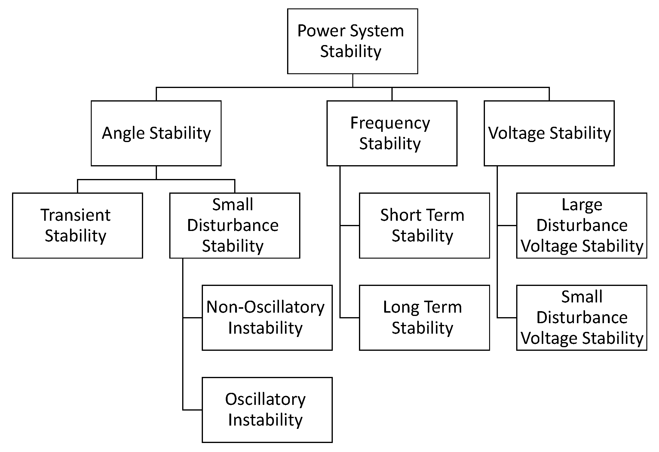
2. Power System Stability

Power system stability is defined as the system’s ability to remain in operating equilibrium, and it can be categorized as shown in Figure 1. There are three main categories [21,22]: angle stability, frequency stability, and voltage stability.

2.1. Angle Stability

All power system machines must be synchronized to maintain equilibrium. The machine’s ability to maintain synchronization is called its angle stability. There are two types of angle stability: transient stability or large-disturbance stability and small angle-disturbance stability. Transient stability or large-disturbance angle stability is the system’s ability to maintain angle synchronism when subjected to a severe disturbance. On the other hand, an event that has a small impact on the system is called small-disturbance stability. Instability caused by a small disturbance can take two forms, either a rotational angle increases through an aperiodic mode due to insufficient synchronizing torque, or oscillations with increasing amplitude occur due to inadequate damping torque [21,22]. Ideally, the power transferred between any source and load bus in a connected power system is given by [23,24]:

$$P=\frac{V_S{V}_L}{X_{Ln}}sin\left(\delta \right)$$

(1)

where $V_S$—voltage at the source bus, $V_L$—voltage at the load bus, $X_{Ln}$—line impedance, and $\delta$—power angle, which is the difference between the source bus and the load bus voltage angle. The maximum power transfer is when the power angle is 90 degrees; if the power angle grows beyond 90 degrees, the system will lose its ability to control angles and power flows. Typically, the power angles between connected buses are less than 10 degrees [25].

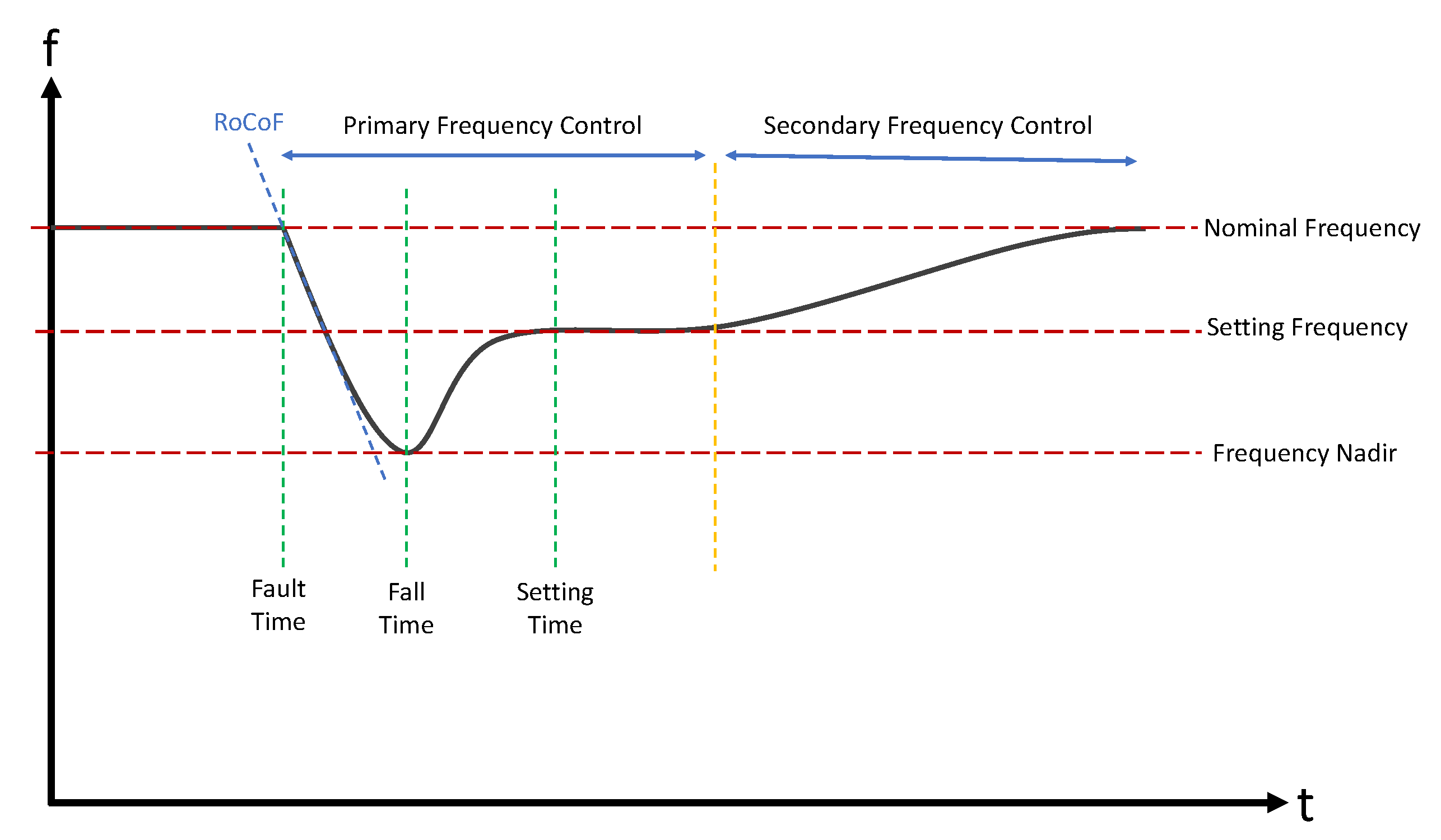
2.2. Frequency Stability

Frequency stability is the ability of the power system to maintain a steady frequency when upsets happen to the power system, resulting in an imbalance between generation and load. Instability occurs when the system frequency continues swinging after the upsets, resulting in tripping of generator units or load. The upsets also affect power flow, voltages, and other system variables; therefore, processes, control, and protections, not modeled in conventional transient stability or voltage stability studies, take actions to protect the system. These processes are slow, such as boiler dynamics, or only act after extreme system conditions, such as protection tripping generators. In an extensive interconnected power system, the most common situation is when a fault causes a system to split into islands. In this case, there will be an imbalance between the generation and the load, which may cause load loss to reach a steady frequency. During the frequency correction action, the activated processes and devices will range from milliseconds to several minutes [23]. In normal frequency deviation under normal conditions, the frequency limit varies in the range of ±0.03 Hz from the reference value. If the system frequency is 60 Hz, the normal range is 59.97 Hz to 60.03 Hz. These variations are normal and frequently occur due to the varying nature of the load. If the frequency deviation exceeds the deviation limit by 1 Hz, this is called an abnormal frequency deviation [25]. An automatic generation control (AGC) system operates at a much higher level of control than a governor. Where a governor control system monitors and controls only one generator, an AGC system monitors a section of the power system, known as a balancing authority area, and controls multiple generators. Governor control is often referred to as primary frequency control, while AGC is referred to as secondary frequency control [25]. Figure 2 summarizes the concept of frequency deviations. The right side of the figure illustrates typical deviations during normal system conditions. If the frequency limit is in the range of ±0.03 Hz, it is called the time correction range, and the AGC corrects the frequency. The governor’s response will enter if the frequency deviation is from ±0.03 Hz to ±1 Hz. The left side of the figure illustrates larger frequency deviations. If frequency deviations are larger than ±1 Hz, automatic protection systems typically operate to minimize damage to the system’s equipment [25].

The frequency fall (frequency nadir) value is the minimum frequency reached after upsets occur to a power system. The time taken from fault time to frequency fall is called the fall time. The setting frequency is the value after the primary frequency control stabilizes the system. The rate of change of frequency (RoCoF) depends on the system inertia. Figure 3 shows the frequency response including the time-frame control reactions [26]. The swing equation is usually used to represent the dynamic frequency response, and it can be expressed as follows [27]:

$$\frac{2H}{f_s}\frac{df}{dt}=\frac{P_m-P_e}{S}=\frac{\Delta P}{S}$$

(2)

where H is the system inertia, $f_s$ is the nominal frequency, $\frac{df}{dt}$ is the rate of change of frequency (RoCoF), $\Delta$P is the difference between the mechanical power input ($P_m$) and the electrical power output ($P_e$), and S is the nominal rating of the system. Frequency response and fall-based frequency response after tripping of generation can be expressed as follows [26,28]:

$$f_{response}\left(\frac{MW}{Hz}\right)=\frac{G_{Lost}}{f_{Nominal}-f_{Setting}}$$

(3)

$$f_{fallBase}\left(\frac{MW}{Hz}\right)=\frac{G_{Lost}}{f_{Nominal}-f_{fall}}$$

(4)

where $G_{Lost}$ is the generation lost in the power system, $f_{Nominal}$ is the nominal frequency value, $f_{Setting}$ is the setting frequency value, and $f_{fall}$ is the frequency fall value.

2.3. Voltage Stability

Voltage stability is the system’s ability to maintain a steady and acceptable voltage. The reactive power Q directly affects the voltage [23,29]. Most loads are inductive, which means they absorb reactive power from the power system. In the case of load tripping, the system’s reactive power will increase; hence, the system voltages will increase. On the other hand, the synchronous generators and PV generation provide reactive power to the power system, which causes the voltages to reduce in the case of generation tripping [30].

3. Energy Storage System

ESSs play a key role in controlling the power in an electrical system. Energy sources such as conventional generators can supply the demand according to customer needs. On the other hand, RES’s output power changes continuously depending on variables such as solar radiation; thus, it is better to store the extra energy and use it when needed. ESS can provide better economic performance and a more stable system [6]. The ESS has multiple purposes, such as power source, load shaving, and stability improvement, in addition to decreasing hydrocarbon emissions, thereby improving air quality [6,31].

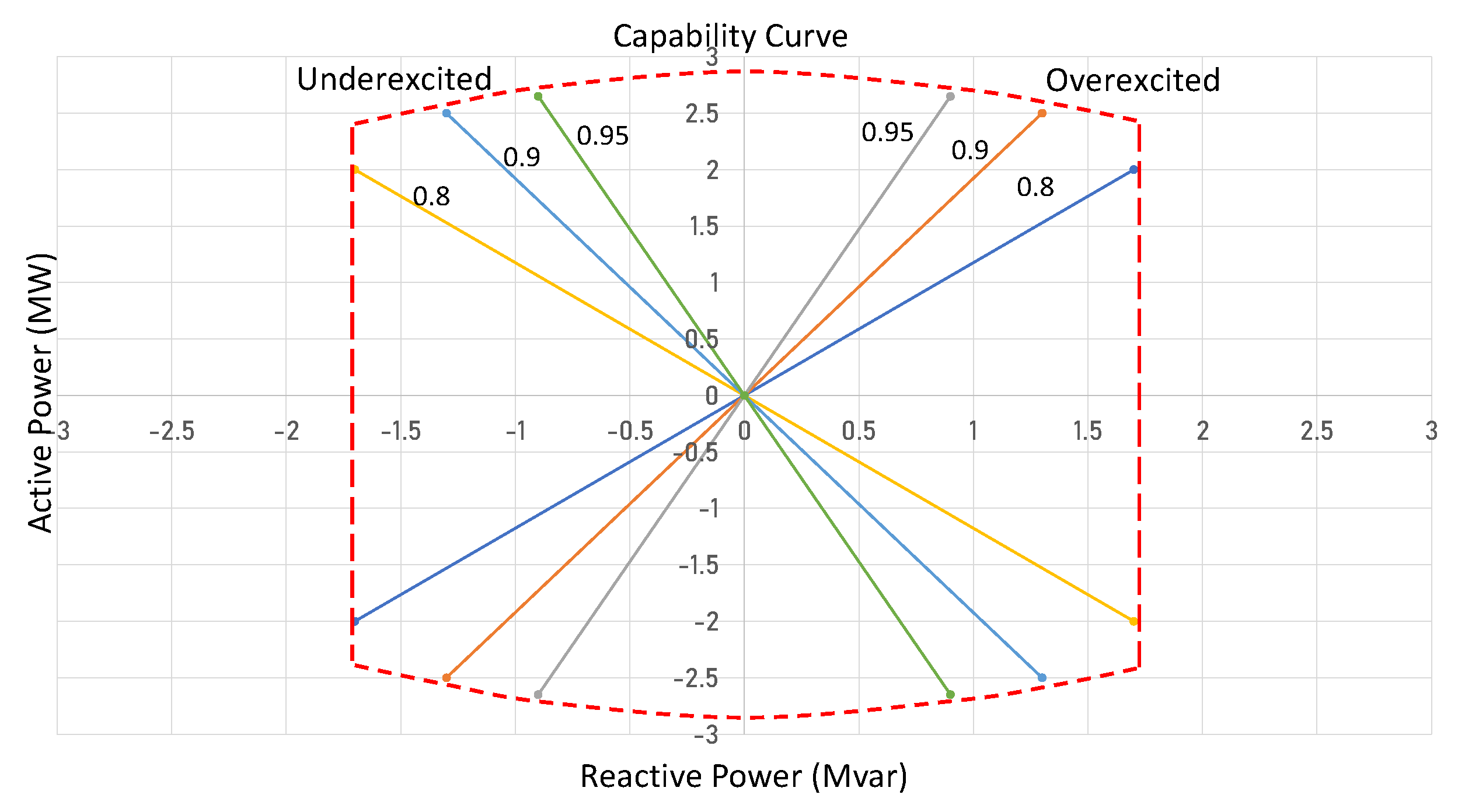
3.1. Capability Curve of BESS

The capability curve of a BESS is defined as the region of charging and discharging, which creates a four-quadrant curve. The shape of the curve is almost symmetrical, as shown in Figure 4 [18]. However, sometimes the design of the BESS is required to limit the capability curve; for example, it limits the losses in the power plant. In such cases, the curve becomes asymmetrical.

3.2. Active Power Frequency Control

Applying conventional droop characteristics to the BESS’s control is an efficient method to provide active frequency control to the system. Transmission planners should specify the boundary of the capability curve (droop setting, dead-bands, and other response characteristics). The droop is almost symmetrical, so the response remains nearly the same, regardless of operation mode. The BESS is considered to be the primary frequency control. The speed of response depends on the primary frequency needed, and the maximum response is determined by the BESS’s state of charge (SOC) [18].

3.3. Reactive Power Voltage Control

The BESS should enhance the voltage stability during normal and abnormal conditions by charging and discharging operations [18].

4. Static BESS Modeling

Figure 5 shows a single-line diagram of a BESS connected to the microgrid [18]. To simplify the BESS static model, we will consider one 132 kV busbar, two 300 V busbars as generator buses, two 132/0.3 kV delta–delta transformers, and two conventional generators.

For steady-state power flow modeling of a BESS, we will consider the following aspects [18]:

4.1. Charging and Discharging Operation

For the P${}_{min}$ value, the equivalent BESS generator charging capability should be set to a negative value for the active power limit. On the other hand, P${}_{max}$ is a positive value representing the discharge capability.

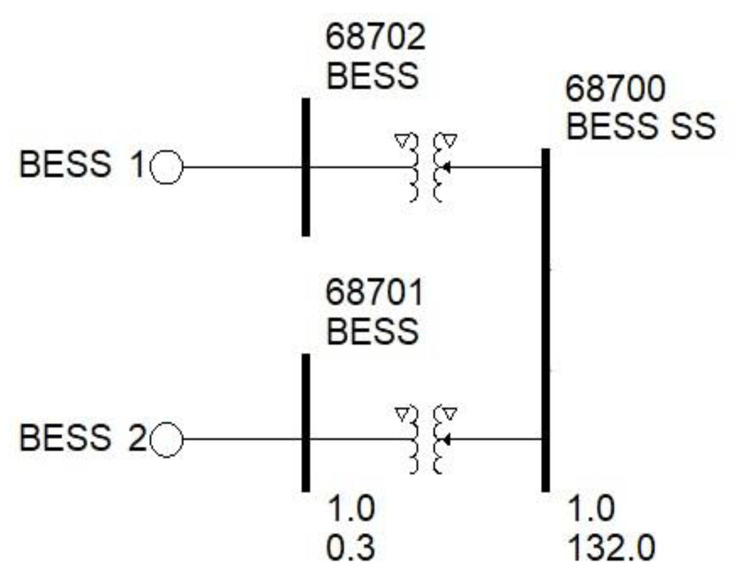
4.2. Point of Voltage Control and Frequency Control

Depending on the Rafha system’s needs, the BESS’s control system will operate with frequency control priority; hence, the limitation of RES’s installation depends on the frequency and active power limit during contingencies.

5. Dynamic BESS Modeling

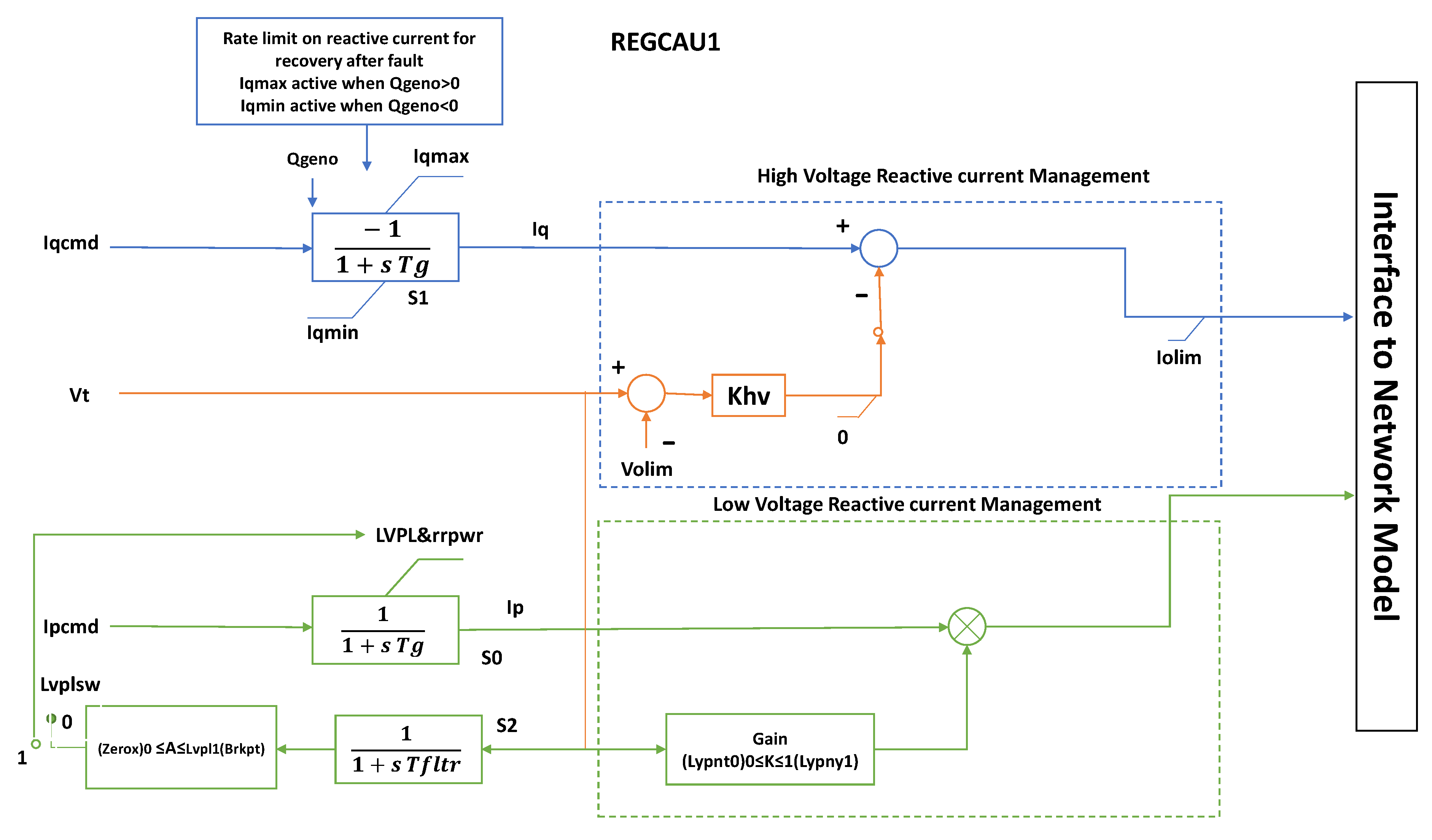
The latest standardized library model to represent a BESS is shown in Figure 6. This model simulates a plant’s overall dynamic behavior. The BESS model is designed and built in the PSS/E platform using the WECC generic model. The model consists of three control modules: plant control, electrical control, and converter control. The frequency and voltage controls are with the electrical control model.

The following modules represent the dynamic behavior of a BESS:

• REGCAU1 module:
  This represents the inverter interface to the power system. REGCAU1 receives the active and reactive current command, with terminal voltage as feedback, and outputs the active and reactive current that will be injected into the grid [32]. The REGCAU1 module shown in Figure 7 can be used to model different RES, such as wind or solar plants.
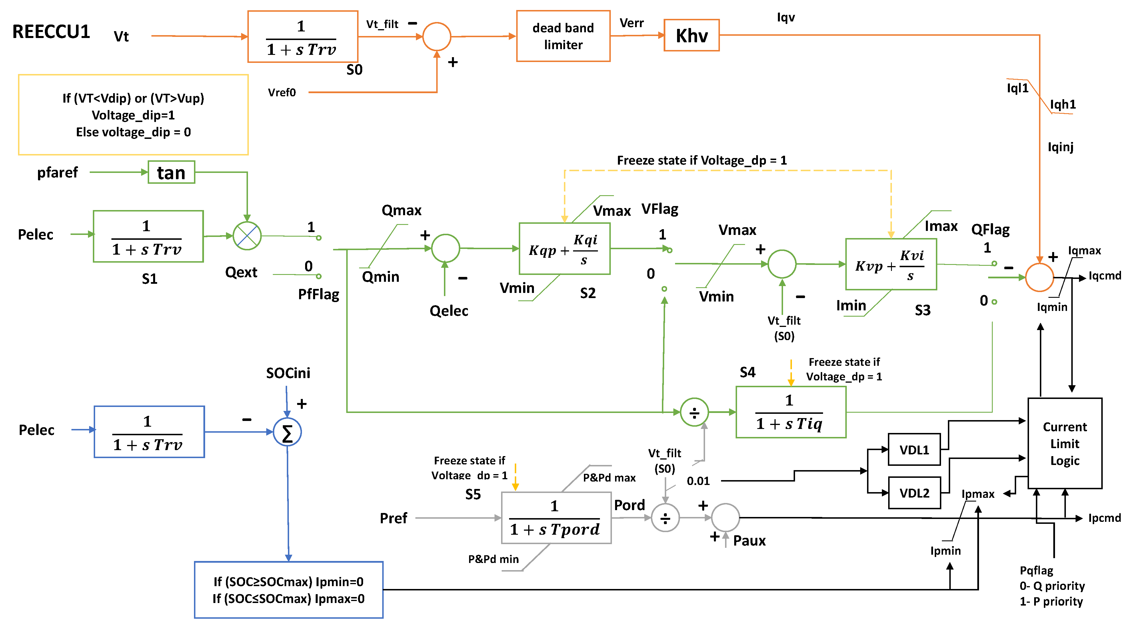
• REECCU1 module:
  REECCU1 is the electrical control module, and it is suitable for BESSs since it can operate the active and reactive power in the four quadrants if the SOC of the BESS allows it. The REECC shown in Figure 8 represents the control of the inverter. The input signals are the active power reference, reactive power reference, and feedback signal of the terminal voltage, which are taken from the REPCAU1 and REGCAU1 modules. The outputs are the active and reactive current commands, which go to the REGCAU1 module [32].
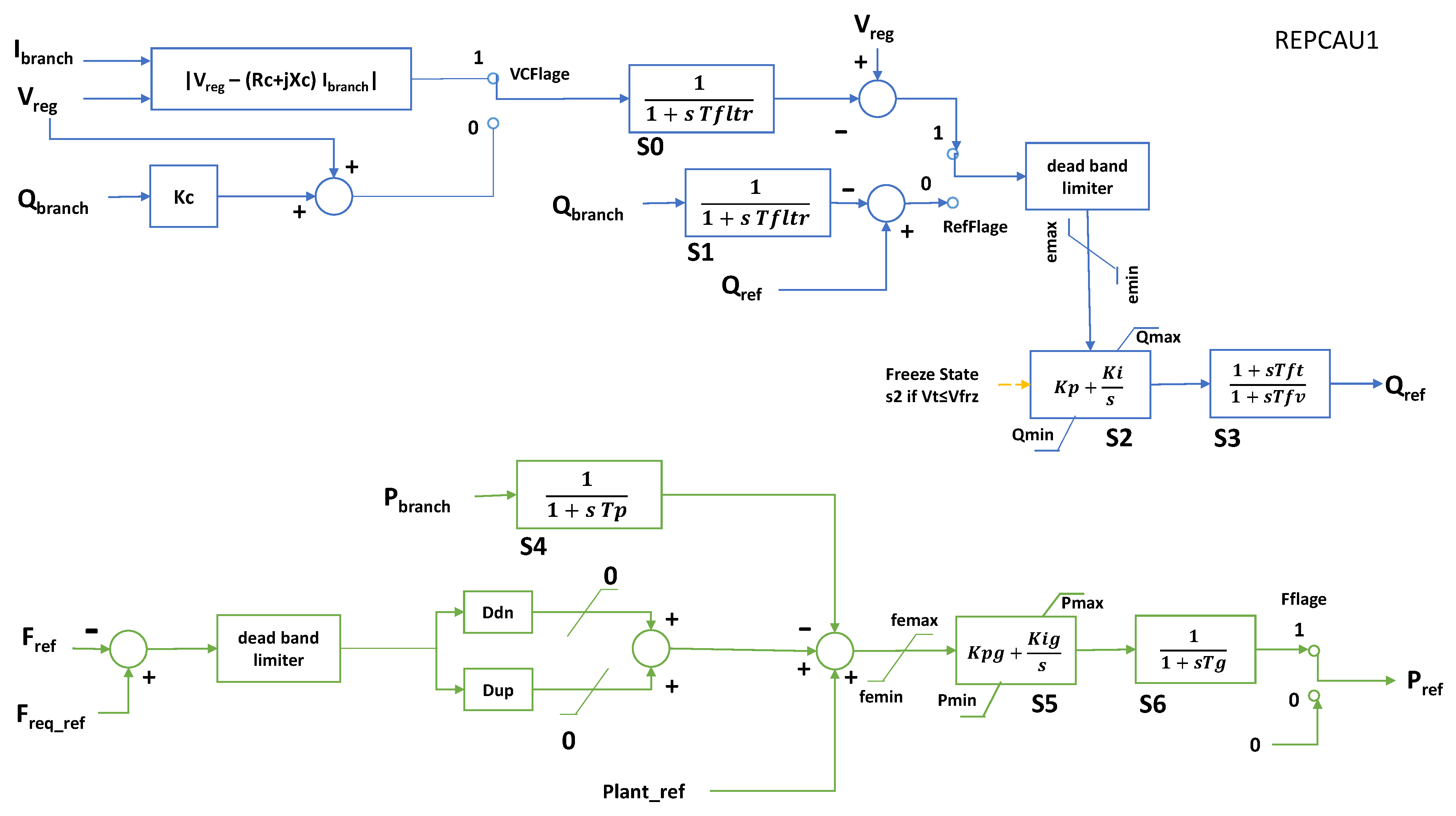
• REPCAU1 module:
  This represents the plant controller. Its inputs are the system voltage and the output reactive power to control the voltage at the plant level. Moreover, it inputs the system frequency, and the output is the active power entering to control the active power [32]. In addition, this module provides active and reactive power signals to the REECCU1 module, as shown in Figure 9. In addition, it can be used as a plant controller in other RES models.

Dynamic values of the BESS are used in the WECC benchmarking model [16,17,18]. However, the model data and the PI controller values have been tuned to meet the Rafha microgrid’s requirements. The dynamic model limitation values will change depending on the BESS’s capacity, but the PI controller values will be the same. Finally, to change the BESS’s location, the BESS’s dynamic reference values will be changed. The data and the dynamic values of the generators, PV generation, and load will be discussed later, in Section 6.

6. Results and Discussion

This section presents the results of the Rafha system utilizing a BESS. It compares it with the base case to see the effect of connecting a stand-alone BESS to the system from a stability perspective, using the PSS/E platform. Further, this section discusses the increasing BESS capacity and its influence on system stability. It represents the spinning reserve capacity range estimated for the Rafha grid, provided by National Grid SA [33]. In addition, the section investigates the effect of changing the BESS’s location on the system stability. Finally, the economic impact of utilizing the BESS is addressed.

6.1. Rafha System Base Case

Rafha is an electrically isolated city in northern Saudi Arabia. The Rafha system has three voltage levels (132 KV, 33 KV, 13.8 KV). Loads and generators are on the low voltage side (33 KV, 13.8 KV). In 2025 it is planned to increase the system load and we will assume that PV generation will be added to the Rafha system. After adding the load and PV generation to the grid, the power system stability system will be affected and may not meet the system requirements. In the base case, the Rafha system consists of five substations: substation A, substation B, substation C, substation D, and PV substation. Substation A contains seven conventional generators, the PV substation consists of solar generation, and the rest are load substations. The base case is established by National Grid SA [33], which has presented a simulation of the Rafha system for the summer of 2025, including the dynamic values of the generators, PV generation, and load, assuming that Rafha is still isolated. The case assumes maximum demand in the summer of 2025, as shown in

Table 1. Forecasted peak load in Rafha.

Substation	Voltage (KV)	Load (MW)	Load (Mvar)	Load (MVA)
Substation A 132/33 KV	33	49.6	19.84	53.42
Substation B 132/13.8 KV	13.8	70.6	28.24	76.04
Substation C	132	60.6	24.24	65.27
Substation D	13.8	50.0	17.00	52.81
Total		230.8	89.32	247.54

.

6.2. Rafha System with Connecting BESS

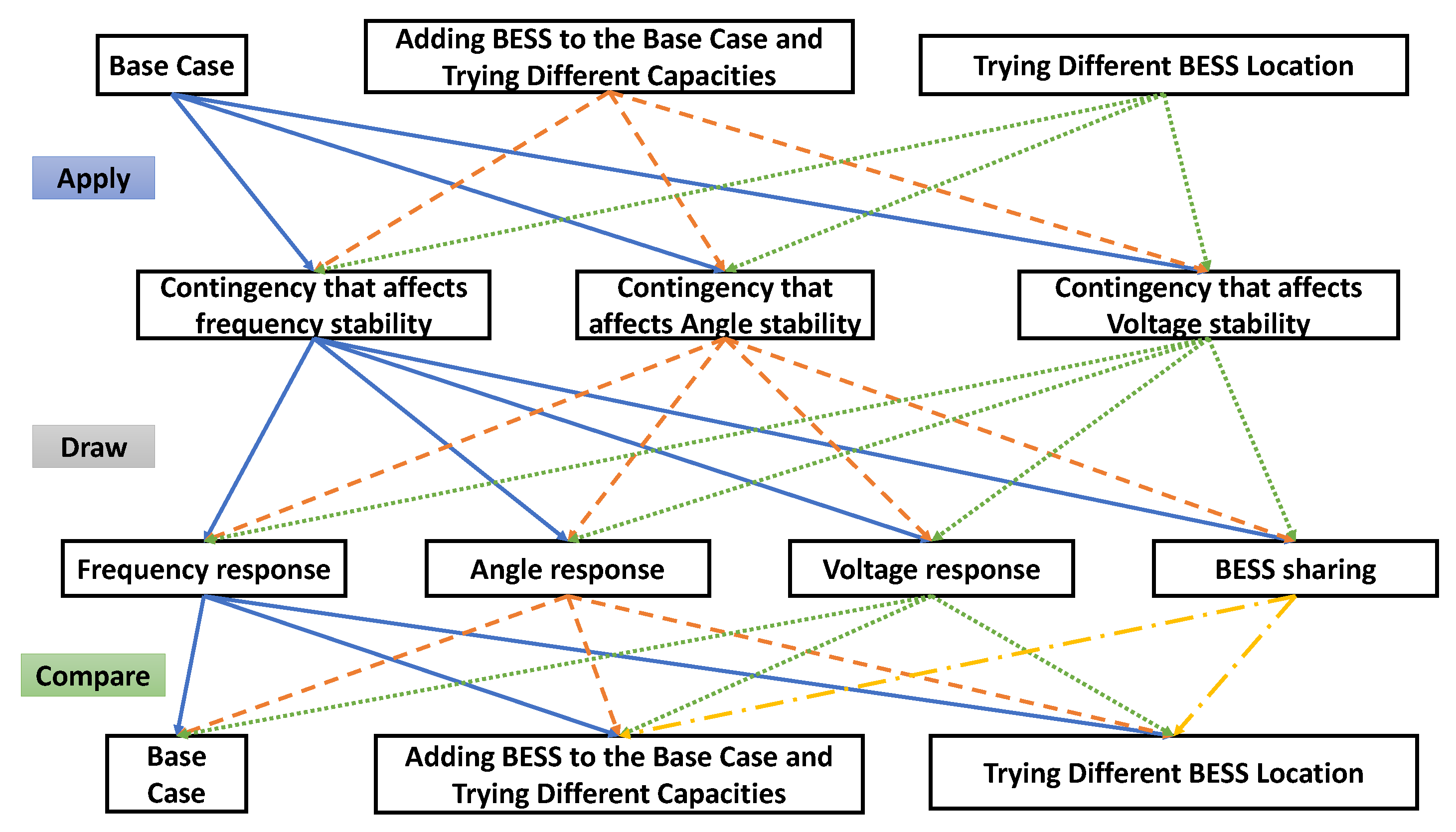
The Rafha system with BESS connecting to the substation B is shown in Figure 10.

Table 2. Generators in service.

Generator	Substation	P${}_{\mathit{G}\mathit{e}\mathit{n}}$ (MW)	P${}_{\mathit{M}\mathit{a}\mathit{x}}$ (MW)	P${}_{\mathit{M}\mathit{i}\mathit{n}}$ (MW)	Q${}_{\mathit{G}\mathit{e}\mathit{n}}$ (Mvar)	Q${}_{\mathit{M}\mathit{a}\mathit{x}}$ (Mvar)	Q${}_{\mathit{M}\mathit{i}\mathit{n}}$ (Mvar)
GT 1	Substation A	20	33	0	1.4903	29	−12
GT 2	Substation A	27	30	0	1.5775	29	−12
GT 3	Substation A	32	76	0	3.5597	65	−37
GT 4	Substation A	35	70	0	4.3533	65	−37
GT 5	Substation A	35	76	0	3.6506	65	−37
PV 1	PV substation	20	81	0	0	0	0
PV 2	PV substation	20	81	0	0	0	0
PV 3	PV substation	20	81	0	0	0	0
PV 4	PV substation	20	81	0	0	0	0
BESS 1	BESS substation	1.8143	2.5	−2.5	0.5074	2.5	−2.5
BESS 2	BESS substation	1.8143	2.5	−2.5	0.5074	2.5	−2.5

shows the generators in service and the generators dispatch. Moreover,

Table 3. Shunt and FACTs.

Shunt/FACTs	Substation	Steps	Q${}_{\mathit{G}\mathit{e}\mathit{n}}$ (Mvar)	Q${}_{\mathit{M}\mathit{a}\mathit{x}}$ (Mvar)	Q${}_{\mathit{M}\mathit{i}\mathit{n}}$ (Mvar)
Capacitor 1	Substation D	1	7	7	0
Capacitor 2	Substation D	1	7	7	0
Capacitor bank	Substation B 132/13.8 KV	3	21	21	0
SVG	PV substation	-	47.5	75	−75

shows data from reactive power components.

6.3. Methodology

As shown in Figure 11, the methodology for investigating the effect of the BESS’s size and location starts by creating the base case and cases with different BESS capacities and locations. After issuing the cases, contingencies are applied that include tripping a generator, simulating a fault, and losing a load. These contingencies affect the frequency, angle, and voltage stability of the Rafha microgrid. Then, the system’s frequency, angle, and voltage response are drawn. Finally, the results are compared to examine how the BESS’s size and location affects the Rafha system’s stability.

Table 4. Cases to test performance.

Contingency	Different Capacity/without BESS	Different Locations
Tripping of PV1 generation	Case 11	Case 21
Fault at GT1 in substation A	Case 12	Case 22
Tripping of substation D load	Case 13	Case 23

states the different contingencies that were performed to investigate the BESS’s influence on the Rafha system’s stability.

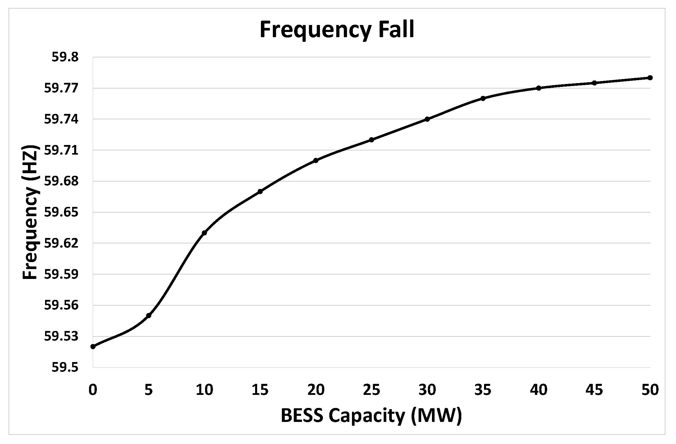
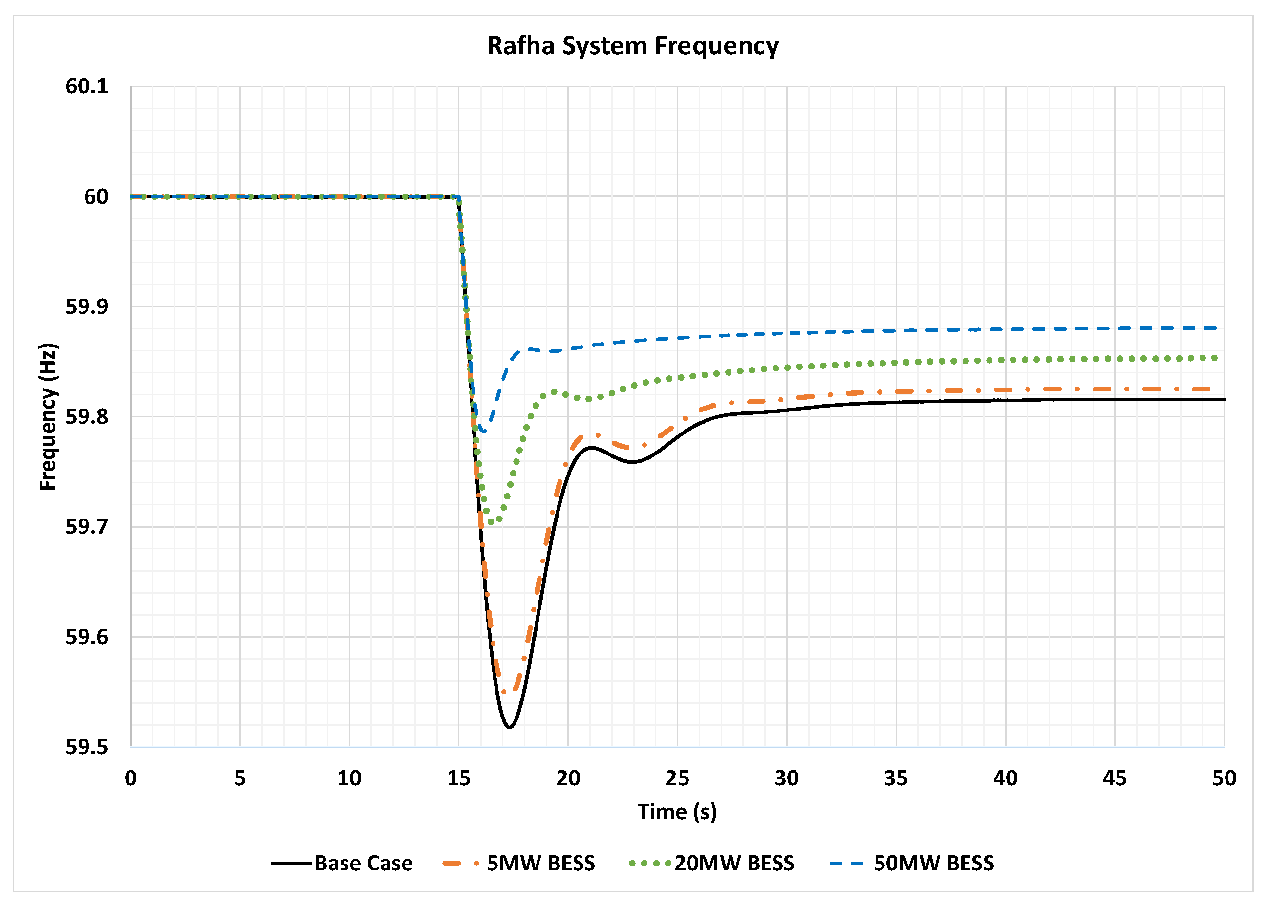
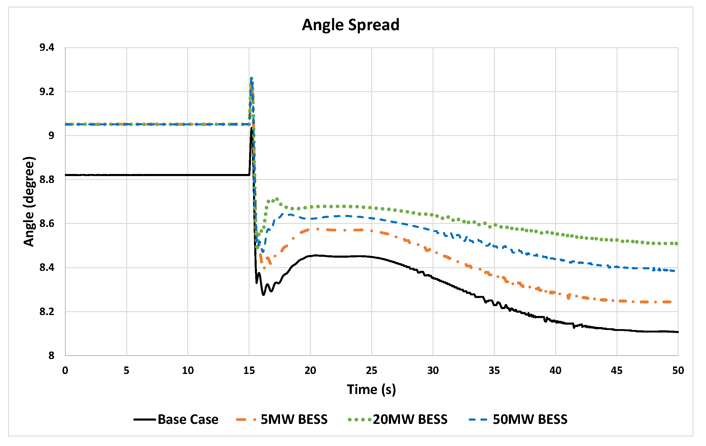
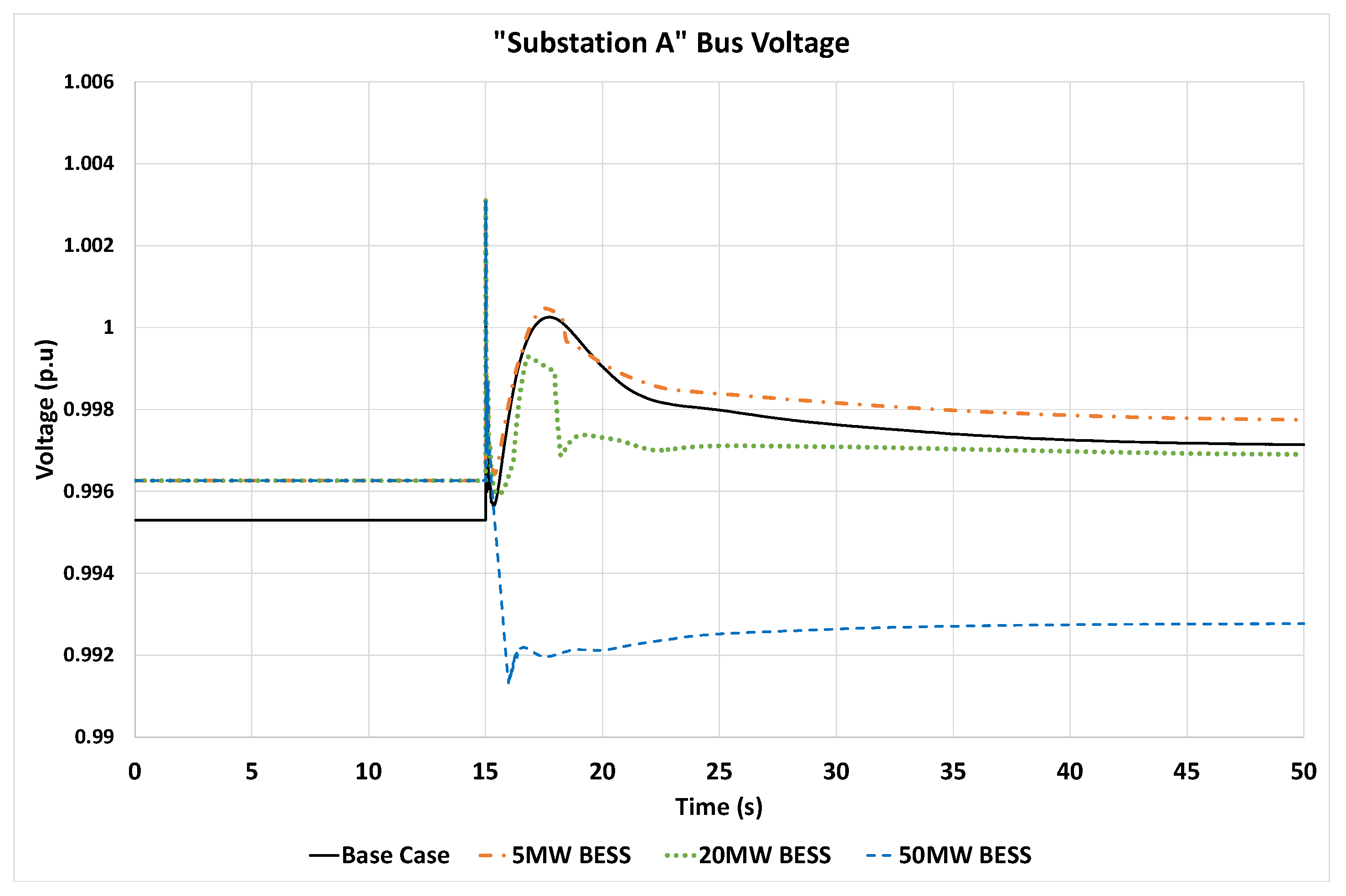
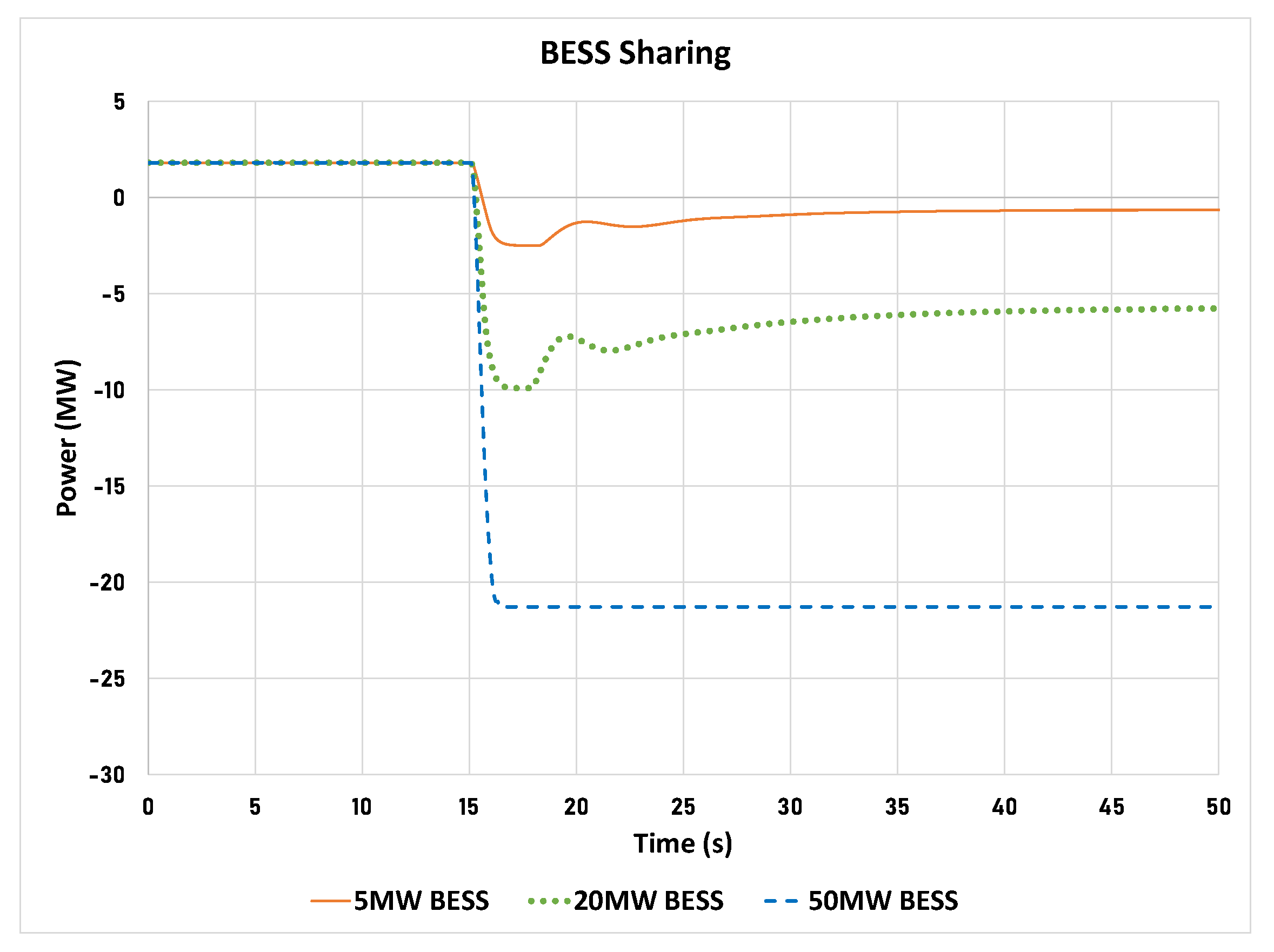
6.4. Testing System Performance with Different BESS Capacities and without BESS

The spinning reserve, as per the grid code in National Grid SA [33], is equal to the generation of the largest two units in the power system. Thus, the reserve of BESS and generators should equal the sum of the generation for the two largest units in the Rafha microgrid. Between 5 and 50 MVA of the BESS’s capacity should be utilized to meet the reserve requirement. Rafha’s demand forecast is 230 MVA for the summer of 2025. However, the frequency fall values (frequency nadir) during the tripping of one PV generator with different BESS capacities are shown in Figure 12.

Now, the connection of the BESS in substation B will be studied in four cases.

• The system without BESS.
• The system with a 5 MVA capacity BESS.
• The system with a 20 MVA capacity BESS.
• The system with a 50 MVA capacity BESS.

6.4.1. Case 11: Tripping of PV1 Generation

This case assumes that the system runs flat, and that after 15 s PV1’s generation in the PV substation is shut down for some reason. The Rafha system frequency response in all four cases is shown in Figure 13. The under-frequency load shedding (UFLS) starts operating if the frequency reaches 58.8 Hz; however, in the case under consideration, UFLS does not operate, and the secondary frequency control is not simulated since we aim to examine the performance of the BESS on the power system stability. Using Equation (2) to calculate the RoCoF in all cases, the rate remains fixed, which means that the BESS does not contribute to the system inertia. As shown in

Table 5. System response with different capacities.

BESS (MVA)	Fall-Based Frequency Response (MW/Hz)	Frequency Response (MW/Hz)
0	41.7	105.3
5	44.4	111.1
20	66.7	133.3
50	90.9	161.3

, we calculate the frequency response and frequency response fall based on (3) and (4).

Before adding a BESS to the system, disconnecting the PV1 generation causes the system frequency to decrease to 59.82 Hz (setting frequency), with frequency nadir equal to 59.52 Hz, reaching the setting time after 15 s. After connecting the 5 MVA BESS to the system, the frequency setting decreases to 59.83 Hz, with a frequency nadir of 59.55 Hz, reaching the setting frequency after 15 s. When the 50 MVA BESS has been connected, the frequency response improves rapidly: it reaches the setting frequency of 59.88 Hz in 5 s, and the frequency nadir is only 59.78 Hz. On the other hand, connecting the 20 MVA to the system decreases the frequency response performance compared to the 50 MVA BESS. It takes 10 s to reach the setting frequency of 59.85 Hz and frequency nadir of 59.7 Hz.

The angle spread is the difference between the system’s minimum and maximum voltage angles, as shown in Figure 14. As the BESS capacity increases, the angle spread becomes more stable.

The voltage in substation A is shown in Figure 15. A BESS increases the steady-state voltage of substation A in all situations. After tripping PV1, the voltage fluctuates. With a 0 or 5 MVA BESS, the fluctuation persists for 8 s and reaches a steady state less than the base case. On the other hand, with a 20 or 50 MVA BESS, the fluctuation lasts for 5 s and reaches a steady state close to the base case.

As shown in Figure 16, BESS sharing with 5 MVA reaches its maximum value and cannot contribute further. In the case of 20 MVA, BESS shares 10 MW (5 MW each), while the power lost is 20 MW. If the BESS is 50 MVA, it contributes 14 MW, which is 70% of the lost power.

6.4.2. Case 12: Fault at GTI in substation A

This case assumes that the system runs flat, and that after 15 s generator GT1 in substation A has a terminal fault for three cycles of 0.05 s. The generator does not trip after the fault. The Rafha system’s frequency response in all four cases is shown in Figure 17. The 50 MVA BESS provides the fastest response (by 5 s); the rest of the BESSs provide almost the same response rate. The angle and voltage responses for all BESS capacities remain the same since it is a transient fault and a BESS does not provide inertia to the system.

6.4.3. Case 13: Tripping of Substation D Load

This case assumes that the system runs flat, and that after 15 s of double lines substation D trips. The Rafha system’s frequency response in all four cases is shown in Figure 18.

The BESS improves frequency response. If the BESS is equal to 50 MVA, the frequency after load tripping of substation D (52.81 MVA) increases by 0.5 Hz, while without the BESS, it increases by up to 1.1 Hz. In addition, it reaches a steady state near the base case. The angle spread is shown in Figure 19. The BESS with a capacity of 50 MVA results in a more stable angle response than the rest of the cases. The voltage in substation A is shown in Figure 20.

The voltage recovery time for the cases with no BESS and the 5 MVA BESS is 7 s, but the voltage recovery time for the 50 MVA BESS is only 2 s. The BESS sharing is shown in Figure 21. The 50 MVA BESS charges almost at maximum capacity.

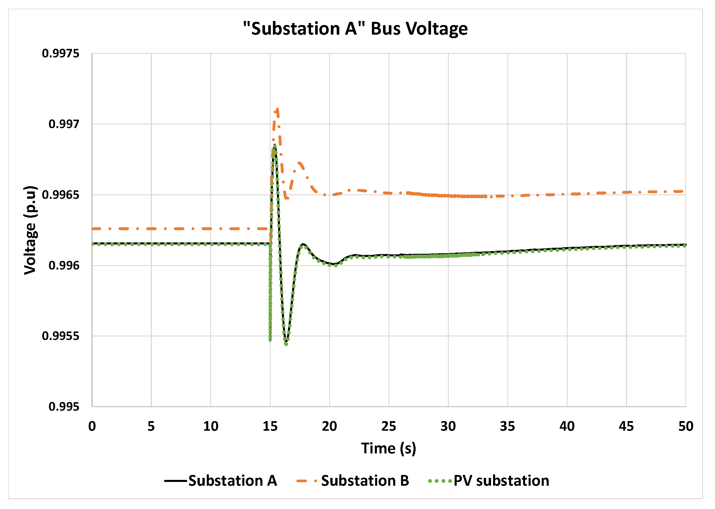
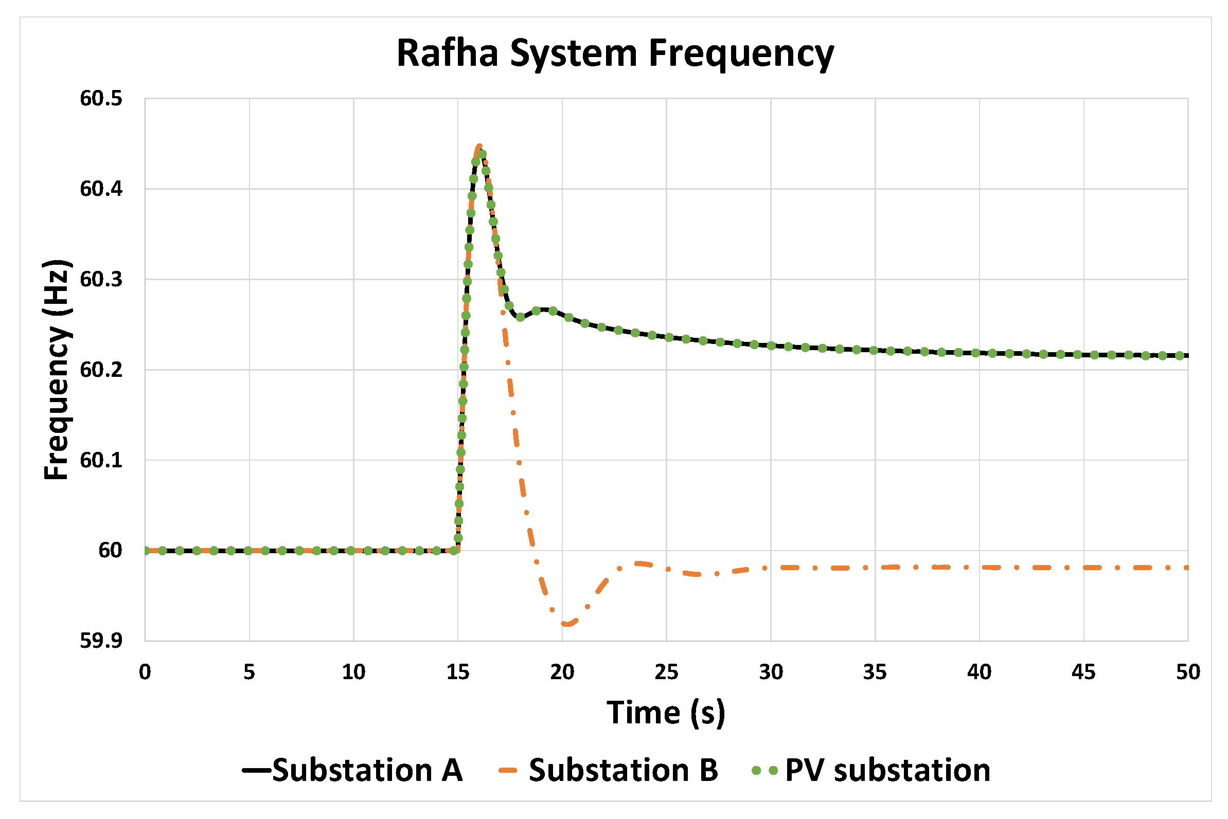
6.5. Testing System Performance with Different Locations

Now, we will keep the BESS capacity at 50 MVA, install the system in different locations, and test the performance in the following locations: substation A, substation B, and the PV substation

6.5.1. Case 21: Tripping of PVI Generation

This case assumes that the system runs flat, and that after 15 s PV1 generation in the PV substation shuts down for some reason. The Rafha system’s frequency and angle response in all three locations remain the same. The voltages, on the other hand, are affected by changing location. When the BESS is utilized in substation B, which is a load bus, it stabilizes the voltage during generation, tripping more than at other locations, as shown in Figure 22.

6.5.2. Case 22: Fault at GT1 in Substation A

This case assumes that the system runs flat, and after 15 s generator GT1 in substation A has a terminal fault for three cycles of 0.05 s, and the generator does not trip after the fault clearance.

The Rafha system’s stability responses in all three locations are the same, since the BESS does not contribute to system inertia. Therefore, the BESS can be located in a high-short-circuit area without significantly impacting the short circuit values. Therefore, changing the location does not affect the system stability in case of faults.

6.5.3. Case 23: Tripping of Substation D Load

This case assumes that the system runs flat, and that after 15 s the double lines of substation D trip. The Rafha system’s frequency response in all three cases is shown in Figure 23.

Locating the BESS in substation B gives a better frequency response. On the other hand, the voltage value will limit BESS sharing at substation A and the PV substation since they are generation buses, and the voltage value will be high after load tripping. The angle spread values of the BESS in all locations are shown in Figure 24. The BESS located in substation A gives a better angle response, since it stabilizes the frequency more than the BESSs in other locations.

The voltage in substation A is shown in Figure 25. Locating the BESS in substation B gives a better voltage response. BESS sharing is shown in Figure 26. As mentioned earlier, the BESS located in substation B charges more than those in the other locations, since the other locations are limited by the voltage value.

6.6. Summary

The BESS will compensate for the contingencies that cause generation loss in the power system and improve the system’s voltage, angle, and frequency stability. The BESS increases the frequency stability during the transient contingencies. Finally, during the loss of load contingencies, the BESS enhances the angle, voltage, and frequency stability.

Table 6. Summary of BESS capacity effect on power system stability.

Case 1	Generation Lost	Transient Fault	Load Lost
Frequency stability	Increase	Increase	Increase
Voltage Stability	Increase	-	Increase
Angle Stability	Increase	-	Increase

shows the summary of the BESS’s effect on the system contingencies. Changing the BESS’s location will impact the voltage stability during the contingencies that cause generation loss. It will also affect the frequency, angle, and voltage stability of the contingencies that cause load loss in the power system.

Table 7. Summary of BESS location effect on power system stability.

Case 2	Generation Lost	Transient Fault	Load Lost
Frequency stability	-	-	Affected
Voltage Stability	Affected	-	Affected
Angle Stability	-	-	Affected

shows a summary of changing the BESS’s location.

7. Conclusions

RES neither provide inertia to the system nor have a primary frequency response capability. With the increasing penetration of RES into the power system, the inertia and spinning reserve will be reduced; hence, system stability will be reduced. Utilizing BESS in the power grid can enhance system stability and provide primary response capability. Installing a higher BESS capacity increases the frequency stability by increasing the frequency setting and fall values and decreasing the fall and setting time values. However, after calculating the RoCoF for different BESS capacities, the RoCoF does not change, since BESS do not have a rotating mass that can provide kinetic energy. Therefore, BESS do not contribute to system inertia, which is why they did not have a high impact on system stability during transient faults. The angle spread and the voltage response of the system is affected by increasing the BESS capacity. If the BESS capacity increases it can generate more active and reactive power. Hence, the angle spread and the voltage after tripping are dampened faster and with lower error, therefore, BESS enhance the steady-state voltages and frequency of the system. Locating BESS near loads helps share their active and reactive power according to their control, although a small effect may appear because of load or generation response. However, BESS near renewable or conventional generation will be highly affected by their controller and may not give the optimal response unless a unique control is implemented (hydride plant) to optimize the performance of BESS considering the plant’s controller effect.

References

1. Wang, M.; Ma, S.; Wang, T.; Zeng, S. Frequency stability analysis of high proportion renewable energy system delivered via DC. In Proceedings of the The 16th IET International Conference on AC and DC Power Transmission (ACDC 2020), Online Conference, 2–3 July 2020; Volume 2020, pp. 675–679. [Google Scholar] [CrossRef]
2. Rahman, S.; Saha, S.; Islam, S.N.; Arif, M.T.; Mosadeghy, M.; Haque, M.E.; Oo, A.M.T. Analysis of Power Grid Voltage Stability With High Penetration of Solar PV Systems. IEEE Trans. Ind. Appl. 2021, 57, 2245–2257. [Google Scholar] [CrossRef]
3. Kpoto, K.; Sharma, A.M.; Sharma, A. Effect Of Energy Storage System (ESS) in Low Inertia Power System with High Renewable Energy Sources. In Proceedings of the 2019 Fifth International Conference on Electrical Energy Systems (ICEES), Chennai, India, 21–22 February 2019; pp. 1–7. [Google Scholar] [CrossRef]
4. Kinoshita, Y.; Kato, D.; Watanabe, M. Power System Simulator to Evaluate Impact of High Penetration of Renewable Energy Resources. In Proceedings of the 2020 59th Annual Conference of the Society of Instrument and Control Engineers of Japan (SICE), Chiang Mai, Thailand, 23–26 September 2020; pp. 571–576. [Google Scholar] [CrossRef]
5. Amrouche, S.O.; Rekioua, D.; Rekioua, T. Overview of energy storage in renewable energy systems. In Proceedings of the 2015 3rd International Renewable and Sustainable Energy Conference (IRSEC), Marrakech, Morocco, 10–13 December 2015; pp. 1–6. [Google Scholar] [CrossRef]
6. Koohi-Fayegh, S.; Rosen, M. A review of energy storage types, applications and recent developments. J. Energy Storage 2020, 27, 101047. [Google Scholar] [CrossRef]
7. Divya, K.; Østergaard, J. Battery energy storage technology for power systems—An overview. Electr. Power Syst. Res. 2009, 79, 511–520. [Google Scholar] [CrossRef]
8. Urpelainen, J.; Van de Graaf, T. The International Renewable Energy Agency: A success story in institutional innovation? Int. Environ. Agreem. Politics Law Econ. 2015, 15, 159–177. [Google Scholar] [CrossRef]
9. Ayadi, F.; Colak, I.; Garip, I.; Bulbul, H.I. Targets of Countries in Renewable Energy. In Proceedings of the 2020 9th International Conference on Renewable Energy Research and Application (ICRERA), Glasgow, UK, 27–30 September 2020; pp. 394–398. [Google Scholar] [CrossRef]
10. Jäger-Waldau, A.; Huld, T.; Bódis, K.; Szabo, S. Photovoltaics in Europe after the Paris Agreement. In Proceedings of the 2018 IEEE 7th World Conference on Photovoltaic Energy Conversion (WCPEC) (A Joint Conference of 45th IEEE PVSC, 28th PVSEC 34th EU PVSEC), Waikoloa, HI, USA, 10–15 June 2018; pp. 3835–3837. [Google Scholar] [CrossRef]
11. Ali, A.; Alsulaiman, F.A.; Irshad, K.; Shafiullah, M.; Alam Malik, S.; Hameed Memon, A. Renewable Portfolio Standard from the Perspective of Policy Network Theory for Saudi Arabia Vision 2030 Targets. In Proceedings of the 2021 4th International Conference on Energy Conservation and Efficiency (ICECE), Lahore, Pakistan, 16–17 March 2021; pp. 1–5. [Google Scholar] [CrossRef]
12. Phurailatpam, C.; Rather, Z.H.; Bahrani, B.; Doolla, S. Estimation of Non-Synchronous Inertia in AC Microgrids. IEEE Trans. Sustain. Energy 2021, 12, 1903–1914. [Google Scholar] [CrossRef]
13. Fernández-Guillamón, A.; Gómez-Lázaro, E.; Muljadi, E.; Molina-García, Á. Power systems with high renewable energy sources: A review of inertia and frequency control strategies over time. Renew. Sustain. Energy Rev. 2019, 115, 109369. [Google Scholar] [CrossRef]
14. Kawabe, K.; Yokoyama, A. Effective utilization of large-capacity battery systems for transient stability improvement in multi-machine power system. In Proceedings of the 2011 IEEE Trondheim PowerTech, Trondheim, Norway, 19–23 June 2011; pp. 1–6. [Google Scholar] [CrossRef]
15. Kandil, M.; El-Deib, A.A.; Elsobki, M.S. Enhancing The Power System Transient Stability by Using Storage Devices With High Penetration Of Wind Farms. In Proceedings of the 2020 6th International Conference on Electric Power and Energy Conversion Systems (EPECS), Istanbul, Turkey, 5–7 October 2020; pp. 13–18. [Google Scholar] [CrossRef]
16. Daraiseh, F. Frequency response of energy storage systems in grids with high level of wind power penetration—Gotland case study. IET Renew. Power Gener. 2020, 14, 1282–1287. [Google Scholar] [CrossRef]
17. Force, W.R.E.M.T. Wecc Battery Storage Dynamic Modeling Guideline; Western Electricity Coordinating Council: Salt Lake City, UT, USA, 2016. [Google Scholar]
18. Corporation, N.A.E.R. Performance, Modeling, and Simulations of BPS-Connected Battery Energy Storage Systems and Hybrid Power Plants; NERC: Atlanta, GA, USA, 2021. [Google Scholar]
19. Xu, X.; Bishop, M.; Oikarinen, D.G.; Hao, C. Application and modeling of battery energy storage in power systems. CSEE J. Power Energy Syst. 2016, 2, 82–90. [Google Scholar] [CrossRef]
20. Ramírez, M.; Castellanos, R.; Calderón, G.; Malik, O. Placement and sizing of battery energy storage for primary frequency control in an isolated section of the Mexican power system. Electr. Power Syst. Res. 2018, 160, 142–150. [Google Scholar] [CrossRef]
21. Kundur, P.; Paserba, J.; Vitet, S. Overview on definition and classification of power system stability. In Proceedings of the CIGRE/IEEE PES International Symposium Quality and Security of Electric Power Delivery Systems, 2003, Montreal, QC, Canada, 8–10 October 2003; pp. 1–4. [Google Scholar] [CrossRef]
22. Kljajić, R.; Marić, P.; Glavaš, H.; Žnidarec, M. Microgrid Stability: A Review on Voltage and Frequency Stability. In Proceedings of the 2020 IEEE 3rd International Conference and Workshop in Óbuda on Electrical and Power Engineering (CANDO-EPE), Budapest, Hungary, 18–19 November 2020; pp. 47–52. [Google Scholar] [CrossRef]
23. Farrokhabadi, M. Primary and Secondary Frequency Control; University of Waterloo: Waterloo, ON, Canada, 2017. [Google Scholar]
24. Song, Y.; Hill, D.J.; Liu, T. Network-Based Analysis of Rotor Angle Stability of Power Systems; IEEE: New York City, NY, USA, 2020. [Google Scholar]
25. Zhag, G. EPRI Power System Dynamics Tutorial; Electric Power Research Institute: Palo Alto, CA, USA, 2009. [Google Scholar]
26. Chamorro, H.R.; Orjuela-Cañón, A.D.; Ganger, D.; Persson, M.; Gonzalez-Longatt, F.; Sood, V.K.; Martinez, W. Nadir Frequency Estimation in Low-Inertia Power Systems. In Proceedings of the 2020 IEEE 29th International Symposium on Industrial Electronics (ISIE), Delft, The Netherlands, 17–19 June 2020; pp. 918–922. [Google Scholar] [CrossRef]
27. Bera, A.; Chalamala, B.; Byrne, R.H.; Mitra, J. Sizing of Energy Storage for Grid Inertial Support in Presence of Renewable Energy. IEEE Trans. Power Syst. 2021, 37, 3769–3778. [Google Scholar] [CrossRef]
28. Jeong, S.; Lee, J.; Yoon, M.; Jang, G. Energy Storage System Event-Driven Frequency Control Using Neural Networks to Comply with Frequency Grid Code. Energies 2020, 13, 1657. [Google Scholar] [CrossRef]
29. Alrumayh, O.; Sayed, K.; Almutairi, A. LVRT and Reactive Power/Voltage Support of Utility-Scale PV Power Plants during Disturbance Conditions. Energies 2023, 16, 3245. [Google Scholar] [CrossRef]
30. Adewuyi, O.B.; Shigenobu, R.; Ooya, K.; Senjyu, T.; Howlader, A.M. Static voltage stability improvement with battery energy storage considering optimal control of active and reactive power injection. Electr. Power Syst. Res. 2019, 172, 303–312. [Google Scholar] [CrossRef]
31. Boicea, V.A. Energy Storage Technologies: The Past and the Present. Proc. IEEE 2014, 102, 1777–1794. [Google Scholar] [CrossRef]
32. Industry, S. Model Library PSS®E; Siemens Power Technologies International: Schenectady, NY, USA, 2018. [Google Scholar]
33. Saudi Electricity Company. Rafha Peak Study in the Year 2025; National Grid SA: Riyadh, Saudi Arabia, 2022. [Google Scholar]
Figure 1. Classification of power system stability.
Sustainability 15 13269 g001
Figure 2. Frequency deviations summary.
Sustainability 15 13269 g002
Figure 3. Power system frequency response.
Sustainability 15 13269 g003
Figure 4. Capability curve of 2.7 MVA BESS.
Sustainability 15 13269 g004
Figure 5. Generic power flow model example for a BESS.
Sustainability 15 13269 g005
Figure 6. Block diagrams of WECC for BESS modeling.
Sustainability 15 13269 g006
Figure 7. REGCAU1 generator/converter generic model.
Sustainability 15 13269 g007
Figure 8. REECCU1 electrical controller generic model.
Sustainability 15 13269 g008
Figure 9. REPCAU1 plant controller generic model.
Sustainability 15 13269 g009
Figure 10. Rafha system utilizing BESS.
Sustainability 15 13269 g010
Figure 11. Methodology flowchart.
Sustainability 15 13269 g011
Figure 12. Frequency fall with different BESS capacities.
Sustainability 15 13269 g012
Figure 13. Rafha system frequency response without a BESS and with different BESS capacities with the tripping of PV generation.
Sustainability 15 13269 g013
Figure 14. Angle spread without BESS and with different BESS capacities after tripping of PV generation.
Sustainability 15 13269 g014
Figure 15. The voltage at substation A without BESS and with different BESS capacities after tripping PV generation.
Sustainability 15 13269 g015
Figure 16. BESS sharing without BESS and with different BESS capacities after tripping of PV generator.
Sustainability 15 13269 g016
Figure 17. Rafha system frequency response without BESS and with different BESS capacities with a fault in GT1 after 15 s.
Sustainability 15 13269 g017
Figure 18. Rafha system frequency response without BESS and with different BESS capacities with the tripping of substation D after 15 s.
Sustainability 15 13269 g018
Figure 19. Angle Spread without BESS and with different BESS capacities with the tripping of substation D after 15 s.
Sustainability 15 13269 g019
Figure 20. Voltage in substation A without BESS and with different BESS capacities with the tripping of substation D after 15 s.
Sustainability 15 13269 g020
Figure 21. BESS sharing with different BESS capacities with the tripping of substation D after 15 s.
Sustainability 15 13269 g021
Figure 22. Voltage at substation A in different BESS locations with the tripping of PV generation.
Sustainability 15 13269 g022
Figure 23. Rafha system frequency response in different BESS locations with the tripping of substation D load.
Sustainability 15 13269 g023
Figure 24. Angle spread in different BESS locations with the tripping of substation D load.
Sustainability 15 13269 g024
Figure 25. Voltage in substation A in different BESS locations with tripping of substation D load.
Sustainability 15 13269 g025
Figure 26. BESS sharing in different BESS locations with the tripping of substation D load.
Sustainability 15 13269 g026