Abstract
Climate change mitigation measures are often projected to reduce anthropogenic carbon dioxide concentrations. Yet, it seems there is ample evidence suggesting that we have a limited understanding of the impacts of these measures and their combinations. For example, the Inflation Reduction Act (IRA) enacted in the U.S. in 2022 contains significant provisions, such as the electric vehicle (EV) tax credits, to reduce CO emissions. However, the impact of such provisions is not fully understood across the U.S., particularly in the context of their interactions with other macroeconomic systems. In this paper, we employ an Integrated Assessment Model (IAM), the Global Change Assessment Model (GCAM), to estimate the future CO emissions in the U.S. GCAM is equipped to comprehensively characterize the interactions among different systems, e.g., energy, water, land use, and transportation. Thus, the use of GCAM-USA that has U.S. state-level resolution allows the projection of the impacts and consequences of major provisions in the IRA, i.e., EV tax credits and clean energy incentives. To compare the performance of these incentives and credits, a policy effectiveness index is used to evaluate the strength of the relationship between the achieved total CO emissions and the overarching emission reduction costs. Our results show that the EV tax credits as stipulated in the IRA can only marginally reduce carbon emissions across the U.S. In fact, it may lead to negative impacts in some states. However, simultaneously combining the incentives and tax credits improves performance and outcomes better than the sum of the individual effects of the policies. This demonstrates that the whole is greater than the sum of the parts in this decarbonization approach. Our findings provide insights for policymakers with a recommendation that combining EV tax credits with clean energy incentives magnifies the intended impact of emission reduction.
1. Introduction
The primary objective of this paper is to evaluate the effectiveness of the Inflation Reduction Act (IRA) enacted in 2022 at reducing anthropogenic carbon dioxide (CO) emissions in order to ameliorate the exacerbating incidences of climate change. Today, climate change is one of the biggest challenges confronting the U.S. and the rest of the world. CO emissions from the transportation sector have already become the largest source of greenhouse gas (GHG) emissions in the U.S. According to the U.S. Energy Information Administration (EIA), the U.S. transportation sector had the most significant increase in CO emissions of all sectors in 2021 [1]. Evidently, the amounts of carbon emissions keep growing with significant contributions to climate change [2,3,4].
Prior research highlights why climate change mitigation should become a necessary regulatory component since the incidences of climate change not only are severe environmental problems, e.g., increased heat, drought, and other outbreaks, but also come with detrimental effects on the infrastructures, transportation, air, and water quality, and public health [5,6,7]. Furthermore, the rural economy is sensitive to climate change through its consequences for agriculture, forestry, water resources, energy, and fisheries [8,9]. While the drivers of climate change and its mitigation measures are well-documented [10,11,12,13,14], the extents of the mitigation measures to curtail CO emissions and thus reduce the incidences of climate change are rarely quantified, or seldom evaluated at best.
Significant aspects of the U.S. Government’s IRA are aimed at alleviating the detrimental effects of climate change. The IRA contains the largest investment in addressing climate change in the history of the U.S. The IRA authorized $391 billion in spending on energy and energy-related artifacts. This provision includes $36 billion in tax incentives for EVs with the aim of decarbonizing the transportation sector by providing tax credits and grants. This enactment also provides numerous grants supporting the adoption of clean energy and related infrastructure. While the IRA aims to reduce the total CO emissions by 40% of the 2005 level by 2050, the practical consequence of such carbon reductions that the policy would achieve still remains unclear and not effectively quantified. Hence, it is essential to examine the effectiveness of the IRA to further refine policy making. This examination is on the backdrop of how firms and individuals respond to competitive pressures in the context of regulatory risk, particularly on capacity investments in response to policy and/or competition [15].
Policy modeling is an important tool to assist climate change management strategies, particularly with respect to their short- and long-term effectiveness. Integrated Assessment Models (IAMs) have been used for a variety of applications including the prediction of future emissions, land use, and water supply and demand under different policy scenarios [16,17,18] and the evaluation of climate change mitigation policy [19,20]. Furthermore, the assessment of the climate impacts of emission scenarios is also studied by applying IAMs [21]. IAMs effectively capture the relationships between human activities and natural systems. The insights from these complex models can inform policy-makers to understand the pros and cons of certain policies [22]. For example, a recent study explores the impacts of capital asset transformation on the decarbonization process by bridging between demand-side policies and supply-side goals [23]. Other studies have examined the role of policies on corporate firm-level emissions [24], and the role of uncertainties when modeling for policy analysis [25].
Some previous efforts mainly focused on studying the projected impacts of policies on socioeconomic parameters, such as gas price, electricity price, number of EVs, and population size. For example, an Energy Policy Simulator modeling was adopted to study the impacts of some sub-policies of the IRA on carbon emissions [26]. The results of Mahajan et al. (2022) show that these policies would reduce U.S. carbon emissions by 37–41% below 2005 levels by 2030—however, not all of the IRA policies were modeled in that study, especially the IRA policies that incentivize the use of EV tax credits. This is particularly important because the fuel price is one of the most significant factors that will influence carbon emissions from transportation [27,28,29]. In addition, it is also necessary to consider the combination of different policies to assist future policymaking [30]. Hence, it is crucial to understand how such policies and their combinations in an IRA regime would influence future U.S. carbon emissions.
While the amount of EV tax credits is flexible in practice, the eventual allocation depends on the characteristics of the purchased vehicle. For example, the credit amount is $3750 if the vehicle meets the requirement of the critical mineral only. Another $3750 is added if the vehicle meets the requirement of the battery components. Previous research modeled the EV tax credits as one fixed amount, ignoring the effects of different levels of tax credit [26]. To better assist policymaking, it is essential to understand the marginal impacts of such policy on emissions in terms of cost, so the insights from this study can help decision-makers determine the optimal level of incentives. In this study, we also explore the impacts of different levels of EV credit on CO emissions, indicated by a policy effectiveness index. Moreover, another study also investigates the potential impacts of the IRA on public health, which is directly related to our daily lives [31]. The results indicate that the IRA may provide a firmer foundation for efforts to abate climate change and reduce its negative impacts on public health. Meanwhile, IAMs can potentially be applied to coordinate environmental, climate, energy planning, and air quality management [32,33,34,35]. Thus, it is necessary to understand how the IRA can influence GHG emissions, ultimately improving public health.
Thus, the aims of this study are to further understand how clean energy incentivizing policies and various levels of EV tax credits of the IRA will contribute to carbon emission reduction at the national and state levels, and by energy source. Thus, we explore the policy effectiveness index to understand the strength of the relationship between CO emissions and the costs of emission reduction in the context of an IAM, the Global Change Assessment Model (GCAM). Our results show that individual EV tax credits can only marginally reduce carbon emissions across the U.S. and may result in negative impacts in some states. However, combining policies could enhance mitigation outcomes. These results are somewhat intriguing because, on the one hand, they show that a top-down policy that aims financial investment at emission reductions may not always lead to the expected outcomes. On the other hand, there was evidence from the bottom up that emission reductions may not always provide firms with the financial gains expected of such efforts [36]. Of paramount importance is the understanding that decarbonizing the transport sector would require the persistence of initiatives as detailed in the IRA.
2. Materials and Methods
Overviews of GCAM and GCAM-USA are provided in the following sub-sections, followed by descriptions of our scenario design to project the effectiveness of IRA and test the policy effectiveness index. In this section, we also present our data sources and collections.
2.1. GCAM and GCAM-USA
GCAM is a partial equilibrium model that links the five major systems, the global energy system, water, agriculture and land use, the economy, and the climate sectors, with a suite of coupled gas-cycle, climate models integrated into the model [32,37]. For over 30 years, GCAM has been used to explore the energy and technology pathways, and the projection of future emissions [38,39,40,41]. GCAM has also been used in studies of the impacts of climate change mitigation measures, and testing the effectiveness of specific policies and other designed scenarios [42,43,44]. GCAM enables users to investigate hypothetical scenarios, quantifying the consequences of potential future circumstances. GCAM serves as a means to evaluate the potential effects of various assumptions about future conditions. GCAM takes external “scenario assumptions” related to critical factors like population, economy, technology, and policies into account, and subsequently evaluates how these assumptions impact important scientific or decision-related outcomes.
GCAM is solved in five-year time steps from 2005 to 2100. GCAM operates as a dynamic–recursive model, where decisions made in a specific time period are based solely on the information available during that period. However, the outcomes of those decisions, such as resource depletion and the accumulation of capital stock, have an impact on decisions made in subsequent periods [37,45]. The detailed descriptions of model structures, integrated dynamics, data sources, and solution-made procedures, are presented in the documentation [46]. The GCAM Data System contains diverse datasets while systematically including various future assumptions. Incorporating input data from the GCAM Data System, the GCAM Core serves as the central component driving the dynamic nature of GCAM. GCAM receives a set of initial assumptions and subsequently processes these assumptions to generate a comprehensive scenario encompassing prices, energy conversions, and other transformations, as well as commodity flows across regions and into the future. GCAM encompasses five distinct interdependent systems and their interactions occur within the GCAM Core.
Within GCAM, the energy system framework includes depictions of both the energy supply and demand sectors for each geographical region. This framework also takes into account the interregional trade of primary resources, such as coal, natural gas, oil, and biomass. The main processes of energy systems consist of three main elements: energy resources, energy transformation, and final energy demands. GCAM also includes various types of clean energy. GCAM’s renewable resources include wind, solar, geothermal, hydropower, and biomass. In GCAM energy systems, wind, solar, geothermal, and hydropower are considered only as options for producing electricity and are not available for trading between different regions. Traditional biomass is only used by the building sector in selected regions [46]. The cost of electricity generation from renewable sources consists of the sum of the resource costs, the technology costs, and, in some cases, backup-related costs. These technologies compete within the energy market, where their relative attractiveness is determined by variations in costs.
GCAM also contains a detailed representation of transportation energy use and service demands, with the sector divided into four service demands, including four final demands: long-distance passenger air travel, (other) passenger travel, international freight shipping, and (other) freight [47,48]. Each sector contains up to five nesting levels, corresponding to different modes (e.g., road, rail), sub-modes (e.g., EV, FCEV), size classes, and corresponding technologies. GCAM can be considered as a process model for CO emissions and reductions. CO emissions change over time as fuel consumption in GCAM endogenously changes. GCAM also considers the emissions from road transportation. GCAM outputs include regional technology utilization, fuel use, GHG, and air pollutants or emissions.
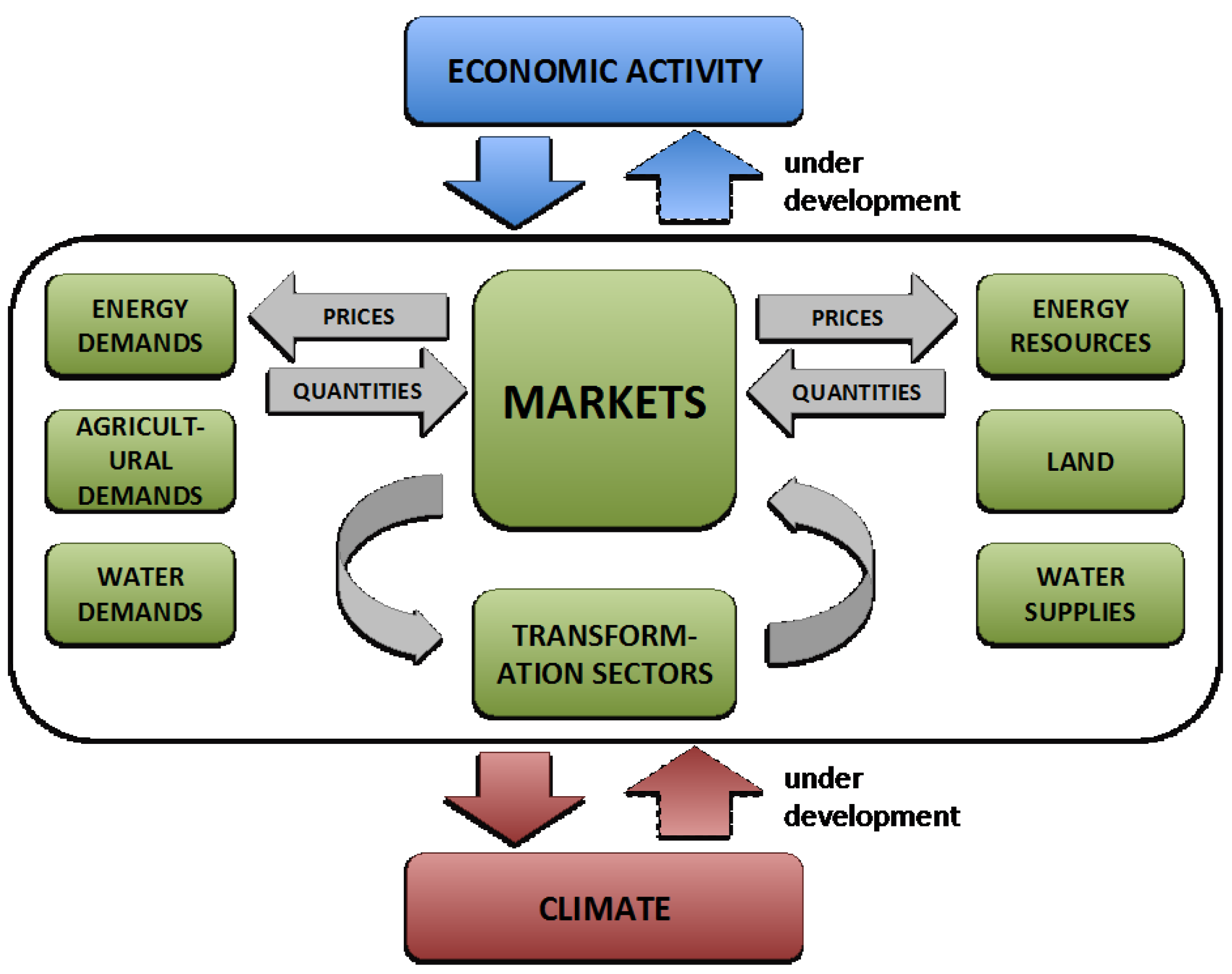
A snapshot of the modeling constructs in GCAM is shown in Figure 1 [49]. The fundamental operating principle underlying GCAM is market equilibrium. Within GCAM, agents utilize price information, along with other pertinent data, to make decisions regarding the allocation of resources. These representative agents are present throughout the model, representing various sectors like regional electricity, regional refining, regional energy demand, and land users who must allocate land for different crops within specific land regions. Markets serve as the means through which these representative agents interact. GCAM intends to determine a set of market prices that balance supply and demand across all these markets within the model. The GCAM solution process involves iteratively adjusting market prices until this equilibrium is achieved. These markets can exist to physical flows such as electricity or agricultural products, but they can also cover other types of goods and services, such as tradable carbon permits.
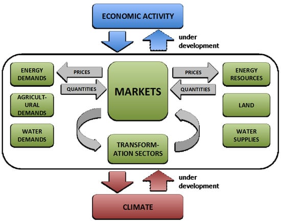
Figure 1.
Conceptual schematic of the operation of the GCAM core.
GCAM-USA is built on the base of GCAM but it subdivides the whole U.S. energy system to represent each of the 50 states and the District of Columbia. GCAM-USA can be used to analyze a suite of state-level, and sectoral-level energy and environmental management policies. These policies can be implemented by applying designed scenarios, such as carbon taxation, emission limits, technology and fuel standards, tax credits or incentives, energy efficiency improvement measures, and clean energy portfolio standards [32].
2.2. Scenario Design
The base scenario in GCAM and GCAM-USA follows a business-as-usual (BAU) condition, which means no specific policy or modification is added. The modified scenarios of this study mainly follow the IRA guidelines, named “Inflation Reduction Act Guidebook” [50]. This report informs the details of the IRA provision and the requirement of incentives. We also want to compare each individual policy implemented with the combination of both policies. The scenarios and descriptions are listed in Table 1 below. The EV tax credit scenario is implemented by modifying the costs of battery electric vehicles (BEVs). The clean energy incentives are designed to reduce both production costs and investment costs of electricity generation based on the production tax credit (PTC) and investment tax credit (ITC) described in the IRA Guidebook.

Table 1.
Designed scenarios.
Scenario 1 is the reference scenario, used as the benchmark to compare with other scenarios to test the effectiveness of certain provisions. Scenario 2 highlights the EV tax credits. In this scenario, we reduce the $7500 of input cost of EVs used in all transportation sectors, such as passenger cars and trucks, and the freight transportation sector. In Scenarios 3a and 3b, a clean energy incentive is applied, which reduces 30% of the input cost of solar, wind, biomass, and geothermal. The only difference is the study period. In Scenario 3a the tax credit is only applied to the production cost. In Scenario 3b, we implement the tax credits only to reduce the investment cost by adjusting the “Fixed-charge-rate” in GCAM, to analyze the effect of energy policy enactment on CO emissions. In Scenario 5, we study a higher level of EV tax credits to analyze the EV policy effectiveness index, as we discussed before. To examine the EV policy effectiveness index, we increase 15% of tax credits on EV costs. In Scenario 6, we implement a higher level of energy incentives to analyze the energy policy implementation, shown in Table 1. To examine the impacts of combo-policy, we implement both EV tax credits and clean energy incentives simultaneously, as shown in Scenarios 4 and 7.
It is imperative to state here that this model incorporates numerous variables that exhibit substantial variations among the states. Given that the objective of this research revolves around examining the potential effects of IRA EV tax credits, the analysis conducted is deterministic but under scenario examinations. Specifically, the policy data is sourced from the IRA-guided book. The values for tax credits and incentives are deterministic and it is important to note that GCAM is not employed for predictive purposes in this study. Instead, GCAM serves as a tool to simulate hypothetical scenarios, allowing for the quantification of the consequences of different assumptions regarding future conditions. Thus, this research is not inclusive of uncertainty analysis.
2.3. Data Collection
The data is collected from the IRA guidance book, which includes the tax credit of each specific program. This guidebook provides a program-by-program overview of the Inflation Reduction Act, including who is eligible to apply for funding and for what purposes. The clean energy section includes an overview of funding. For each funding program, more details are explicitly introduced, such as Tax Mechanism, Base Credit Amount, and Bonus Credit Amount.
2.4. Per Unit Cost of Emission Reduction
To assess the performance of the proposed policies, we define the policy effectiveness index, , an evaluation metric, as the ratio of the change in emissions relative to the change in cost, i.e., the per-unit cost of emission reduction as shown in Equation (1):
In Equation (1), the numerator represents the change in total carbon emissions, which includes emissions from transportation, power generation, and other sectors. The denominator indicates the change in mitigation measures costs reduced by policy implementation. The cost information is contingent upon the type of policy being considered. For example, in the case of the EV tax credit scenario, our emission reduction costs pertain to the costs of EVs. To avoid the scale issues, we use a percentage of the change instead of the true or actual values. In other words, is informative of how a one percentage decrease in either EV costs or clean energy costs will affect the change in total emissions. The margins, and , imply that is a strictly increasing function of policy effectiveness, i.e., a higher value of indicates a more efficient implemented policy.
It is important to note that we have not utilized specific dollar amount changes as the denominator of the policy effectiveness index since there are certain challenges with employing this metric at this juncture [51]. First, the parameters in GCAM undergo a complicated conversion process. For instance, the conversion of costs related to EVs entails a series of intricate steps. Each of the steps may result in some scaling differences. Specifically, an EV tax credit conversion involves “conversion to 1990 US dollars”, number of passengers per car, average annual distance per car, the lifetime of a car in years, annual discounted rate, etc. Therefore, to levelize such differences, we assess the marginal impacts of policy in terms of reduction costs. Second, the energy investment tax credits realized in GCAM are not quantified in dollars. They are represented by a parameter called “fixed charge rate”, that is a factor used to levelize capital cost. We modify this parameter to equivalently reduce the investment cost of certain clean energies as the IRA guidebook suggested. At this stage, using “per dollar” as the denominator will not be suitable for quantifying the extent to which cost reductions in mitigation efforts translate into final emission reductions.
3. Results and Discussion
In this section, each proposed scenario is implemented and tested in GCAM and GCAM-USA individually. The effectiveness of policies is examined by comparing design scenarios to the reference scenario. The comparison is first carried out at the national level, followed by an assessment of state-level results. The state-level policy scenarios combine PTC and ITC together to examine the effectiveness of clean energy incentives. The state-level policy effectiveness index adjustment is presented and interpreted. The results of each scenario and its corresponding implications are presented below.
3.1. U.S. National-Level CO Emission Reductions
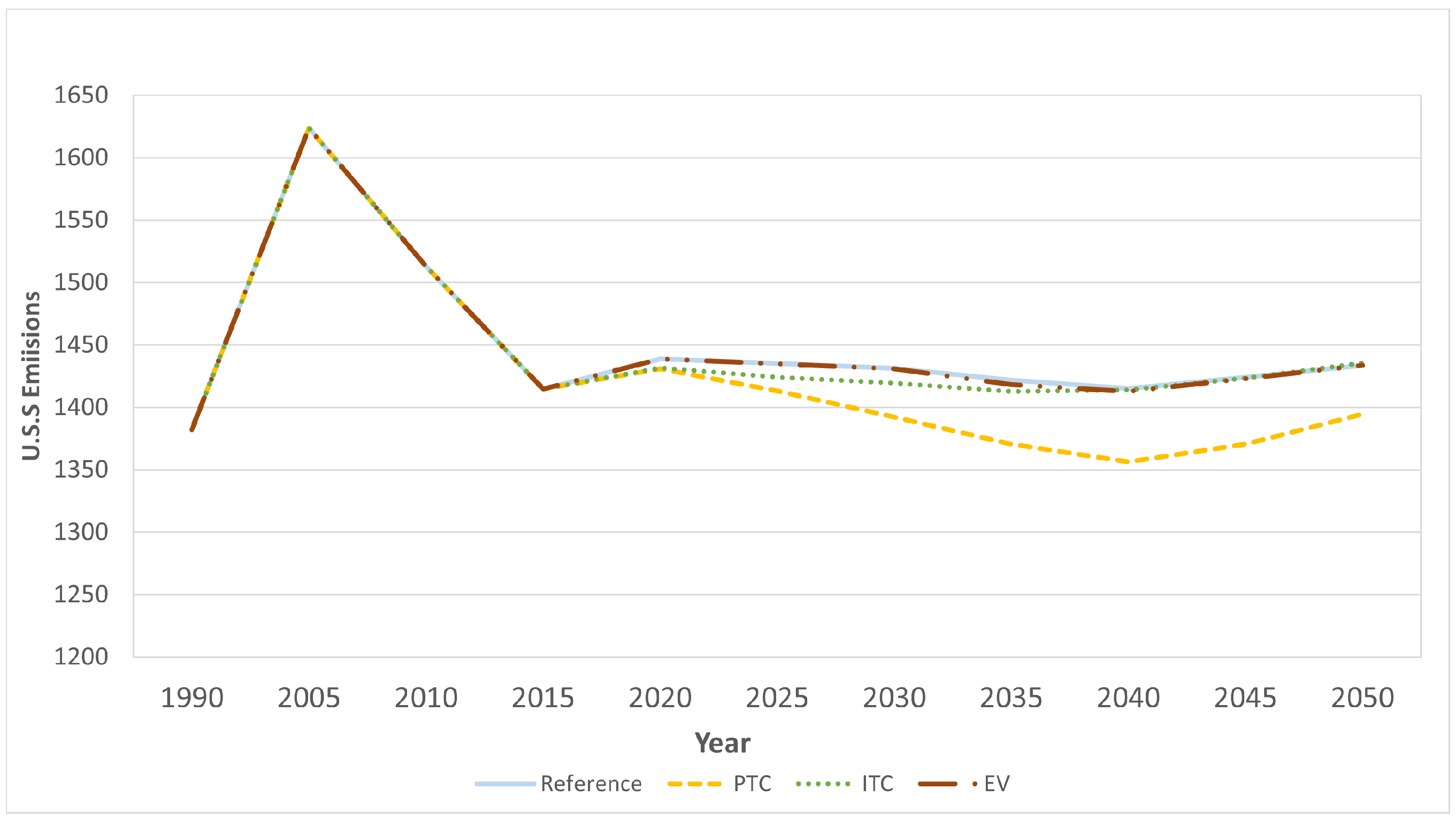
Figure 2 shows the comparisons of CO emissions between the designed scenarios and the reference scenario.
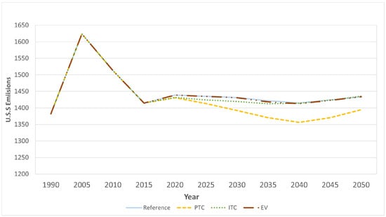
Figure 2.
National-level CO emissions.
This plot depicts the total U.S. national-level carbon emissions of each scenario. The PTC can reduce the highest emission amounts by four percent of the reference scenario when comparing these two results in Year 2030. Additionally, compared with the 2005 level, the ultimate goal that IRA aims to achieve, PTC can reduce 16% of CO emissions. The ITC can only reduce 0.6% of carbon emissions by the Year 2030 and rapidly move back to the reference level by the Year 2040, compared with the reference scenario. The national scale emission plots demonstrate that only PTC can achieve the goal of emission reductions. At the sectoral level, the main emissions are reduced substantially from electricity generation by traditional sources, such as coal and gasoline, according to Figure 3. Subsequently, emissions are reduced from industrial and residential sectors.
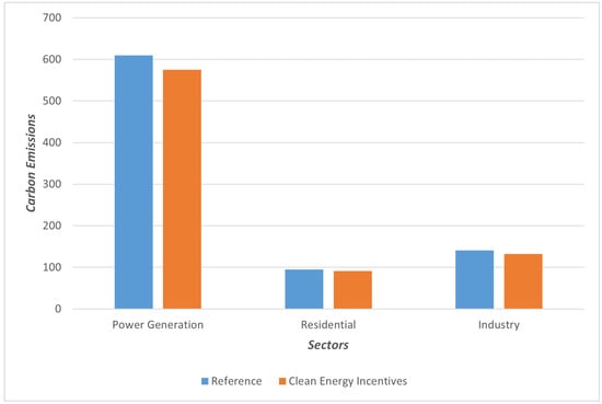
Figure 3.
CO emissions by sectors.
3.2. U.S. State-Level CO Emission Reductions under EV Tax Credits
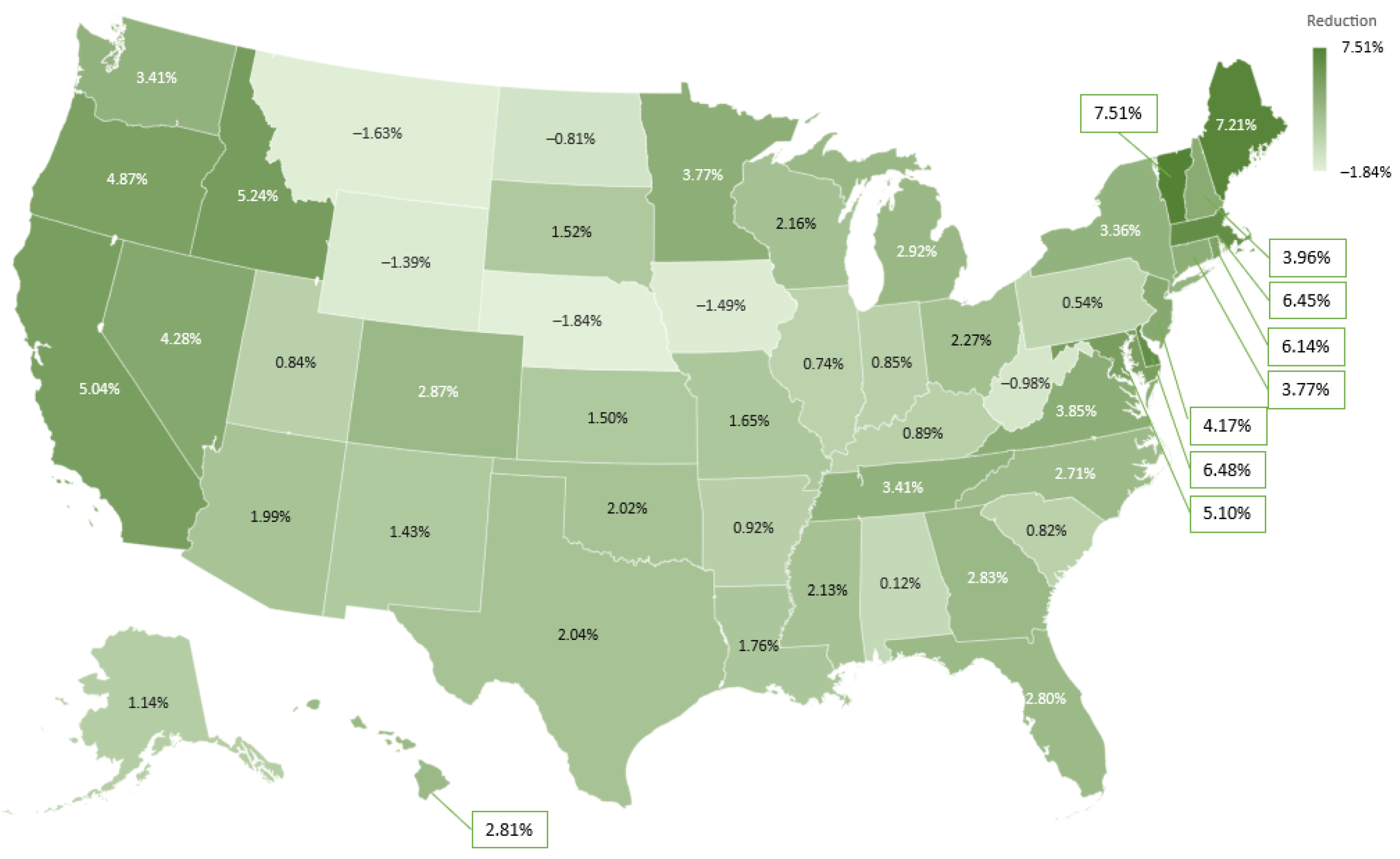
The state-level reductions of carbon emissions achieved by the IRA EV tax credits are shown in Figure 4.
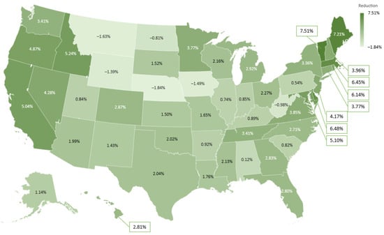
Figure 4.
CO emission reductions by EV tax credits.
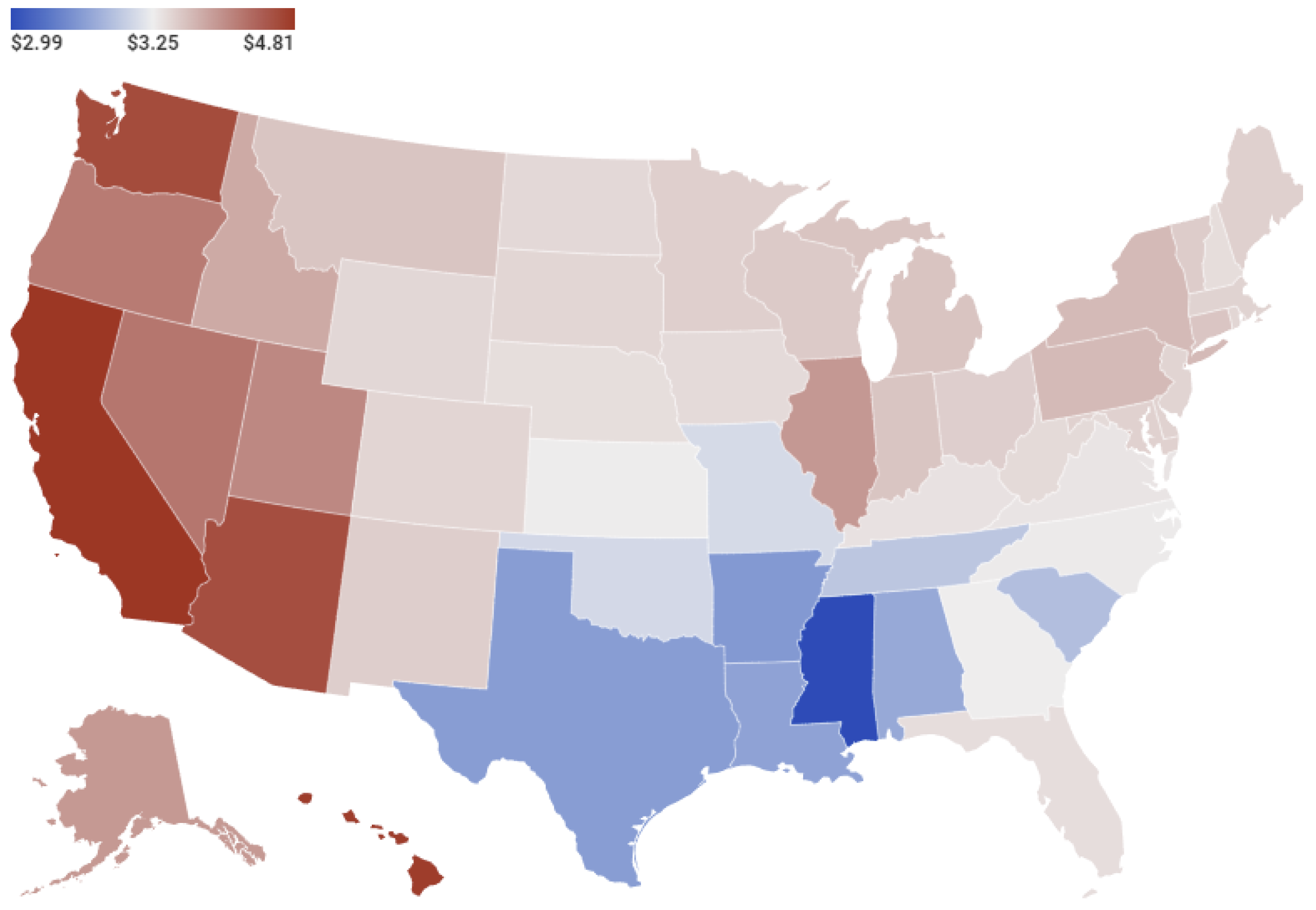
The percentage of emission reductions is calculated relative to the reference scenario, where there is no policy implemented. In this figure, the darker the color is, the higher the reductions that are achieved. Maine state reduces 7.2% of carbon emissions, the highest reductions, by only applying the EV tax credits, followed by California, Idaho, and Oregon. The Pacific region, including Washington, Oregon, California, Nevada, and Arizona, reduces more emissions on average than any other area. Following the Pacific region, the New England area is the second place that reduces high portions of carbon emissions. According to Figure 5, the dark-red-colored states are the areas whose gasoline prices and population are higher than others [52].
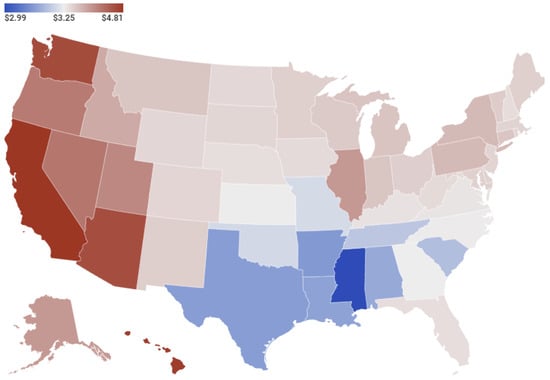
Figure 5.
U.S. state-level gasoline prices [52].
The emissions from the rest of the states are reduced moderately. Another interesting finding is that the carbon emissions of several states increased after enacting EV tax credits, such as Montana, Wyoming, and North Dakota. Montana emits the highest CO, which is 1.63%, compared to the reference scenario. This finding is out of the expectation, showing that EV tax credits result in negative impacts on carbon emissions. It is important to note that the reason behind this result can be attributed to the discrepancy in EV usage among states and the balance of power generation within the power grid. In the context of GCAM-USA, the model calculates energy demand and emission levels by relying on external assumptions regarding state-level factors such as population, GDP, and labor productivity [41,53,54]. However, the amount of electricity generation is balanced among 15 “grid regions”. In the initial step, GCAM-USA assigns the generation of electricity to specific fuel sources within the generation segments. This allocation process utilizes a heuristic method grounded in the concept that the total electricity demand within each horizontal segment should match the supply from each respective segment.
Additionally, the model calculates the proportion of each fuel type within the generation segments at the grid region level and presumes that these proportions remain consistent across all states within a given grid region [55,56].
Furthermore, GCAM-USA computes CO emissions by considering fuel consumption and the carbon content of different types of fuels. As shown in the tables below, it becomes evident that EV tax credits lead to varying levels of emission reduction in individual states reflected by the different levels of increases in EV usage. Nonetheless, when it comes to increased power generation, there is no notable discrepancy among states within the same grid. As emissions from power generation rise in tandem with relatively lower reductions from transportation, EV tax credits can result in adverse effects on specific states.
Specifically, Table 2 shows the outcome of the Northwest Grid. In Montana (negatively impacted by EV tax credits), the improved usage of EVs triggered by tax credits is the lowest among the states in the grid. This leads to the lowest reduction in transportation. Table 3 displays the outcome of Southwest Grid. The results demonstrate the same information that, for Wyoming state, emission reduction from transportation is lower than emission increases in electricity generation. These states provide more power to the grid than required by themselves. Some previous research also shows that the impact of incentives on buyers varies depending on sociodemographic and vehicle choice characteristics [57]. Additionally, another study finds out that acquiring an emission advantage requires that EVs exceed specific aggregate utilization thresholds [58]. Our finding shows that, when the usage of EVs is low, EV tax credits can result in an adverse influence on emission reductions. Hence, EV tax credits result in negative impacts in specific states if EV usage is not significantly improved.

Table 2.
Northwest Grid region results.

Table 3.
Southwest Grid region results.
3.3. U.S. State-Level CO Emission Reductions by Clean Energy Incentives
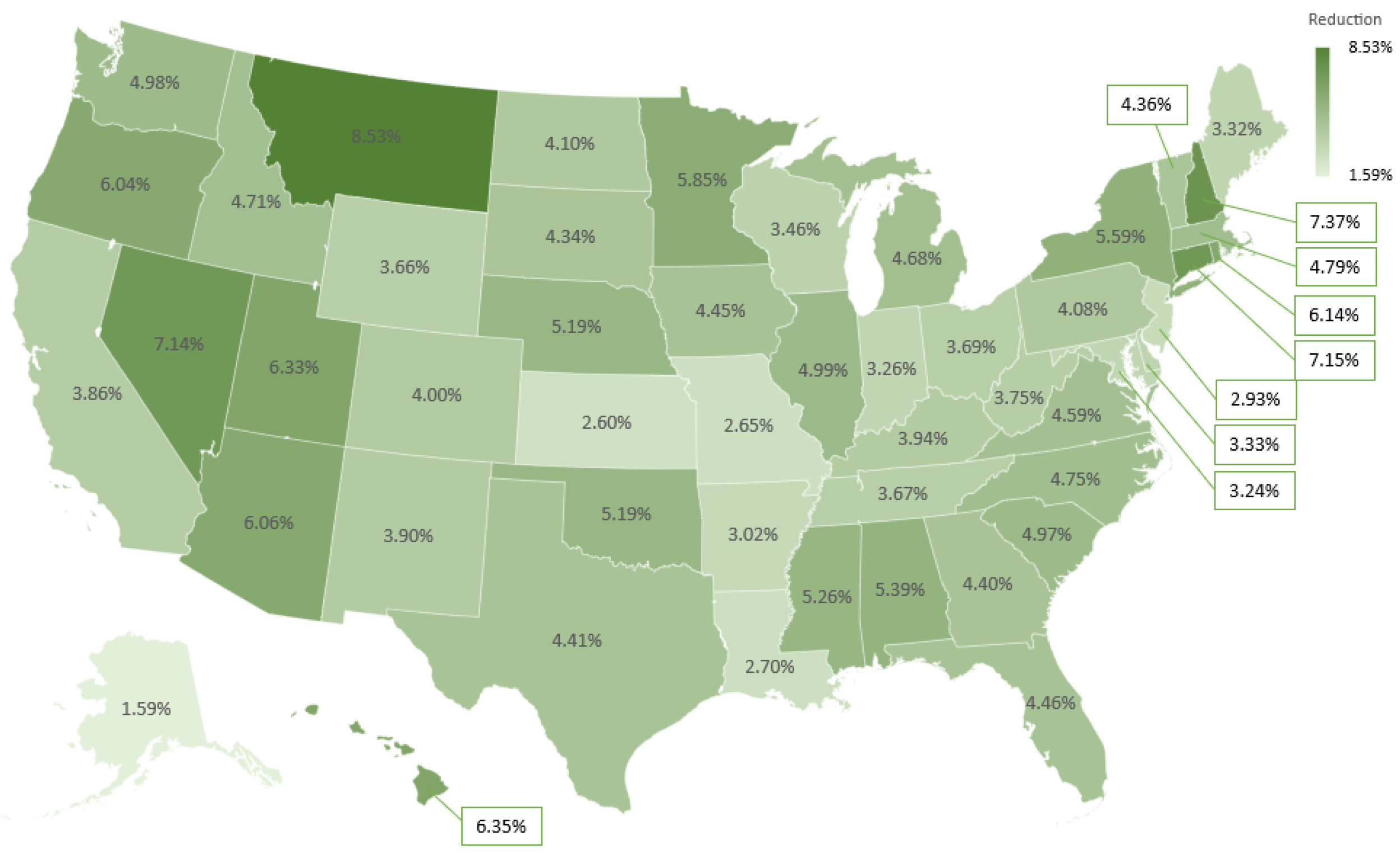
The emissions reduced by clean energy incentives (including both PTC and ITC) are shown in Figure 6 below.

Figure 6.
CO emission reductions by clean energy incentives.
Carbon emissions in all the states are reduced by applying clean energy incentives, especially in Montana. Montana is one of the states that reduce the most emissions. Those states that generate more emissions due to EV tax credits now reduce a greater amount of emissions than other states. Clean energy incentives reduce emissions in some states when EV tax credits cannot. For example, Montana, Wyoming, West Virginia, Nebraska, North Dakota, and Iowa are the states that can benefit much from clean energy incentives but not EV tax credits.
3.4. U.S. State-Level CO Emission Reductions by Combo-Policy
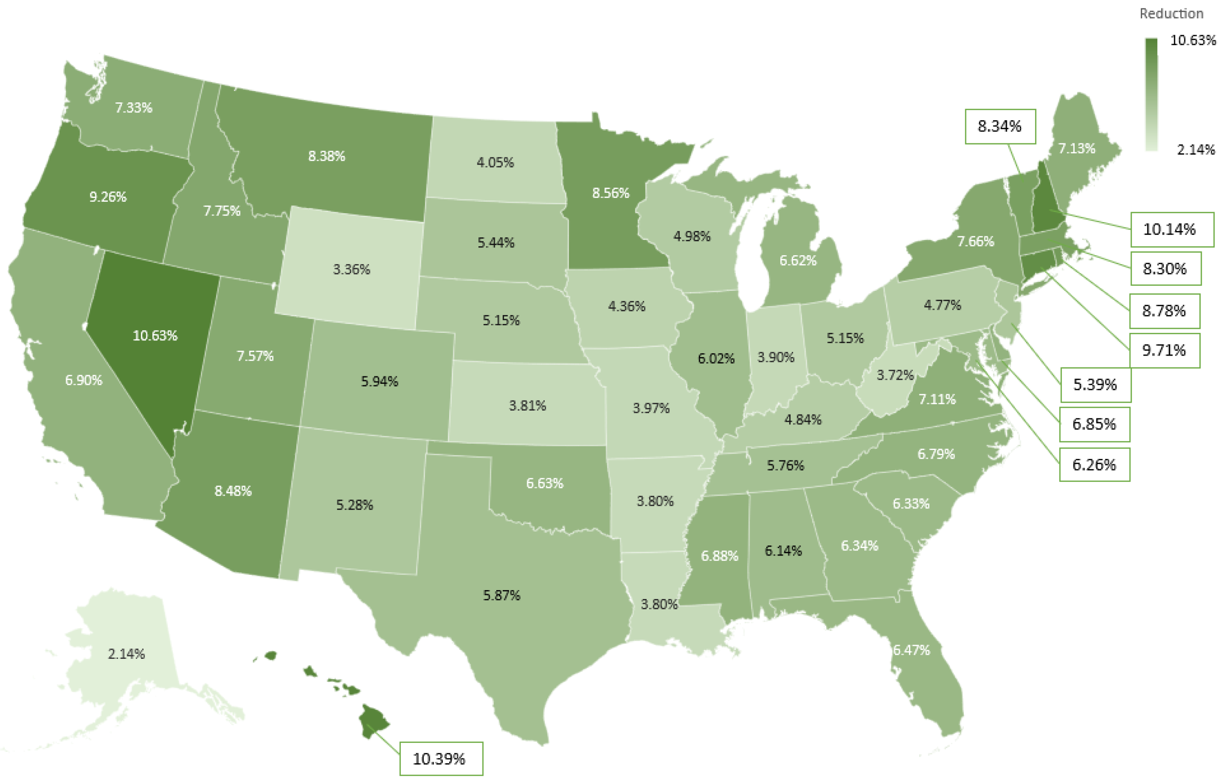
Applying both EV tax credits and clean energy incentives simultaneously into what we term a combo-policy can significantly reduce carbon emissions for all the states. According to Figure 7, the west region, which includes California, Oregon, Nevada, etc., reduces more emissions than other regions.
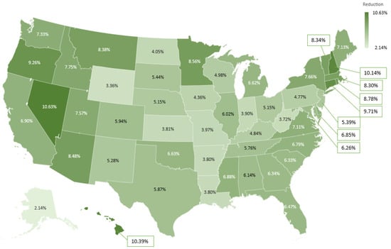
Figure 7.
CO emission reductions by combo-policy.
The southeast region also efficiently reduces emissions. By looking at the middle region, the emissions of Montana state reduced by 8.38%, which is higher than most of the states. In addition, Montana, Wyoming, and North Dakota also reduce more emissions than when applying a single policy. This finding indicates that clean energy incentives can effectively mitigate the negative impacts caused by EV tax credits. Furthermore, our results show that combo-policy can achieve a better performance than the sum of individual policies. For example, individual EV tax credits can help California reduce 4.87% of CO emissions. With the aid of PTC and ITC, the CO emissions are reduced by 6.04% in total. Implementing the combo-policy, including both EV tax credits and clean energy incentives, can reduce 13.8% of total CO emissions, which is higher than the sum of individual policy implementations.
3.5. U.S. State-Level Policy Effectiveness Index of EV Tax Credits
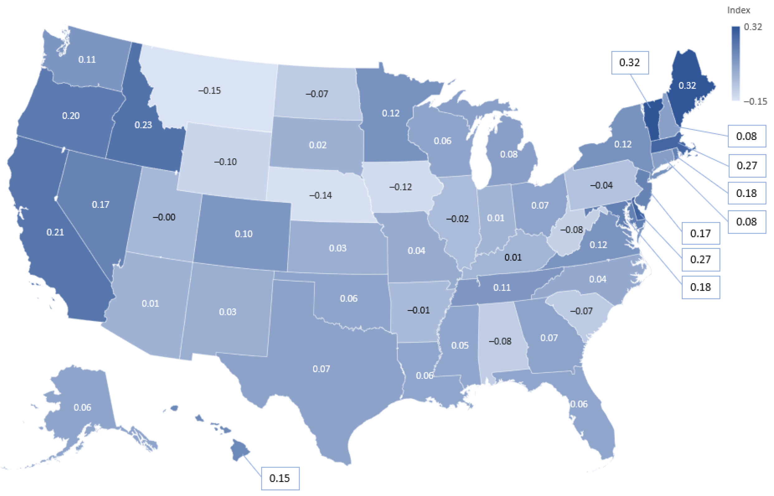
Figure 8 shows the policy effectiveness index of EV tax credits. The number on the plot shows the percentage of emissions reduced by one percent, showing the marginal impacts of reducing mitigation measure costs. As an illustration, let us consider California and Washington. In California, the policy effectiveness index stands at 0.21, surpassing that of Washington. This outcome suggests that reducing the equivalent percentage of EV costs in California results in greater emission reductions. Conversely, a negative value in Montana implies that cost reductions for EVs have led to an increase in carbon emissions. Furthermore, a lower negative value signifies a more substantial increase in emissions.

Figure 8.
Policy effectiveness index of EV tax credits.
The policy effectiveness index of each state shows a positive relationship to the performance of corresponding EV tax credits. For those states that can achieve high emission reductions when implementing EV tax credits, they also obtain a high value on the policy effectiveness index. The states with higher emissions that are caused by EV tax credits also have a negative value on the policy effectiveness index. These findings also indicate that increasing the level of EV tax credits is not feasible to mitigate the negative impacts caused in certain states.
3.6. U.S. State-Level Policy Effectiveness Index of Clean Energy Incentives
Figure 9 shows that greater reduction of the production cost of clean energy can effectively reduce carbon emissions across the U.S.
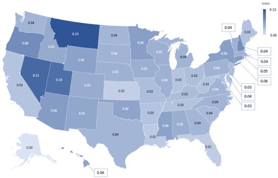
Figure 9.
Policy effectiveness index of clean energy incentives.
Reducing clean energy production costs can always have a positive impact on state-level carbon emissions when reducing clean energy cost. All states have a similar degree of policy effectiveness index, indicated by the similar color across the U.S. except for Montana, Nevada, and Utah. In particular, Montana reaches the greatest policy effectiveness index. This result also shows a similar trend to the emissions reduced by clean energy incentives. A state with higher emissions reduced by policy always has a higher degree of policy effectiveness index.
3.7. U.S. State-Level Policy Effectiveness Index of Combo-Policy
The policy effectiveness index of the combo-policy is shown in Figure 10. By applying clean energy incentives, some states, whose emissions are reduced by EV tax credits, obtain a higher value on the policy effectiveness index. For example, the policy effectiveness of the combo-policy in California is doubled after applying combo-policy, compared to the individual EV policy. This result implies that implementing a combo-policy can enhance the performance of such mitigation measures in terms of the policy effectiveness index. For the states with a negative impact caused by EV tax credits, the policy effectiveness index of the combo-policy is significantly increased. For example, the value on the policy effectiveness index of the combo-policy in Wyoming is increased by six percent. This result indicates that a combo-policy can also mitigate the negative impacts caused by EV tax credits in certain policies. In Montana, in particular, the value of combo-policy effectiveness changes from negative to positive. This result means that reducing one percent of costs can significantly reduce the higher amount of emissions, showing that the combo-policy can effectively enhance both policy performances at the same time.
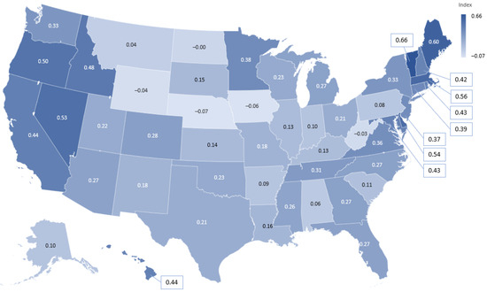
Figure 10.
Policy effectiveness index of combo-policy.
3.8. Numerical Analysis
According to the statistics of numerical results shown in Table 4, both the average of emissions reduced by EV tax credits, 2.52%, and by clean energy incentives, 4.57%, are lower than the combo-policy average. The average reductions of the combo-policy are also higher than the sum of emissions reduced by EV tax credits and clean energy incentives. The standard deviations of each alternative are low. This indicates that these policies’ implementation does not create significant differences among states.

Table 4.
Statistics of state-level results. Note: the is mean value and is the standard deviation.
The average policy effectiveness index of EV tax credits is higher than clean energy incentives. This result shows that the effectiveness of EV tax credits is more sensitive to the level of policy, which means reducing more EV costs can lessen CO emissions. However, the larger value of the standard deviation indicates that the previous observation might not be applicable to all states. The results from the previous section show that individual EV tax credits can cause negative impacts on some states. A higher value of the combo-policy effectiveness index also demonstrates reducing emission reduction costs is more efficient. The larger value of the standard deviation shows the significant differences existing among states across the U.S.
4. Conclusions
A crucial driver for successfully achieving the goals of the IRA is that policymakers must anticipate its projected effects and be able to make the requisite dynamic amendments as the impacts evolve. While qualitative research focuses on identifying the drivers of climate change, quantitative studies use empirical data to examine the relationship between such drivers, or between other socioeconomic parameters and climate change. However, to the best of our knowledge, how effective an enactment would be is less considered in the literature.
This study uses GCAM-USA to evaluate the effectiveness of some of the provisions of the IRA enacted in 2022 using two metrics, i.e., CO emission reduction and the policy effectiveness index. The major provisions in the IRA, i.e., clean energy incentives and EV tax credits, are modeled and evaluated. We draw some important insights that guide future policymaking. For example, several components of the IRA may outperform expectations on carbon emission reduction in some jurisdictions while underperform in others. To be more specific, PTC can unilaterally reduce total CO emissions in the U.S. by 16% of the 2005 level. On the other hand, the ITC can only independently reduce 0.6% of carbon emissions by the Year 2030, with the potential for emission levels to rapidly regress back to the reference level by the Year 2040. However, clean energy incentives can only effectively reduce carbon emissions from conventional fuels in electricity generation. It should be noted here that the challenges relating to policy compliance or monitoring are assumed to be nonexistent. Lower prices of clean energy options can also lead to some emission reduction from the residential sector. We also identified that the positive impact of clean energy incentives may become weakened and even negative over the years.
On the other hand, our results show that individual EV tax credits cannot significantly reduce carbon emissions across the U.S. They may also result in negative impacts in certain states, such as Montana and Wyoming. However, combining energy policies can bring a better performance for both mitigation measures. Carbon emissions in several states increased after enacting EV tax credits, such as Montana, Wyoming, and North Dakota, without clean energy incentives. The results of the policy effectiveness index also indicate that only clean energy incentives can mitigate the negative impacts caused by EV tax credits in some states and improve the effectiveness of EV tax credits in other states. We note here that the effect of technological learning or performance as often noted with clean energy analysis [59,60] are ignored.
Overall, clean energy incentives are one of the most efficient policies to reduce carbon emissions. The government is recommended to spend more money on the most common clean energy development, such as wind, solar, and geothermal. On the other hand, EV tax credits are not always the most effective way to reduce emissions, except when combining with the clean energy incentives simultaneously. A higher tax credit on EVs might result in better performance but is not efficient for all states. Combining two policies can enhance the effectiveness of both policies.
Author Contributions
Conceptualization, T.W. and E.S.; methodology, T.W.; software, T.W.; validation, T.W. and E.S.; formal analysis, T.W.; investigation, T.W. and E.S.; resources, E.S.; data curation, T.W.; writing—original draft preparation, T.W.; writing—review and editing, T.W. and E.S.; supervision, E.S.; funding acquisition, E.S. All authors have read and agreed to the published version of the manuscript.
Funding
This research was funded by U.S. National Science Foundation grant number 1847077.
Data Availability Statement
Data available in a publicly accessible repository that does not issue DOIs. Publicly available datasets were analyzed in this study. These data can be found here: [https://jgcri.github.io/gcam-doc/gcam-usa.html].
Acknowledgments
The authors wish to acknowledge the support of Haewon McJeon of the Joint Global Change Research Institute, Pacific Northwest National Laboratory, University of Maryland and Korea Advanced Institute of Science & Technology (KAIST).
Conflicts of Interest
The authors declare no conflict of interest. The funders had no role in the design of the study; in the collection, analyses, or interpretation of data; in the writing of the manuscript; or in the decision to publish the results.
Abbreviations
The following abbreviations are used in this manuscript: CO2—Carbon dioxide; EV—Electric vehicle; GCAM—Global Change Assessment Model; GHG—Greenhouse gas; IAM—Integrated Assessment Model; IRA—Inflation Reduction Act; ITC—Investment tax credit; PTC—Production tax credit; USA—United States of America.
References
- U.S. Energy-Related Carbon Dioxide Emissions. 2021. Available online: https://www.eia.gov/environment/emissions/carbon/ (accessed on 17 February 2023).
- Shirley, C.; Gecan, R. Emissions of Carbon Dioxide in the Transportation Sector; Congressional Budget Office: Washington, DC, USA, 2022.
- Milovanoff, A.; Posen, I.D.; MacLean, H.L. Electrification of light-duty vehicle fleet alone will not meet mitigation targets. Nat. Clim. Chang. 2020, 10, 1102–1107. [Google Scholar] [CrossRef]
- Zhang, R.; Fujimori, S. The role of transport electrification in global climate change mitigation scenarios. Environ. Res. Lett. 2020, 15, 034019. [Google Scholar] [CrossRef]
- The Effects of Climate Change. Available online: https://climate.nasa.gov/effects/ (accessed on 12 December 2022).
- Kilpatrick, A.M.; Meola, M.A.; Moudy, R.M.; Kramer, L.D. Temperature, Viral Genetics, and the Transmission of West Nile Virus by Culex pipiens Mosquitoes. PLoS Pathog. 2008, 4, e1000092. [Google Scholar] [CrossRef] [PubMed]
- Ebi, K.; Balbus, J.; Kinney, P.L.; Lipp, E.; Mills, D.; O’Neill, M.S.; Wilson, M. Chapter 2: Effects of Global Change on Human Health. In Analysis Of The Effects Of Global Climate Change On Human Health And Welfare And Human Systems; U.S. Environmental Protection Agency: Washington, DC, USA, 2008; Volume 4. [Google Scholar]
- Lal, P.; Alavalapati, J.R.R.; Mercer, E.D. Socio-economic impacts of climate change on rural United States. Mitig. Adapt. Strateg. Glob. Chang. Vol. 2011, 16, 819–844. [Google Scholar] [CrossRef]
- McCarty, J.P. Ecological consequences of recent climate change. Conserv. Biol. 2001, 15, 320–331. [Google Scholar] [CrossRef]
- Gifford, R.; Kormos, C.; McIntyre, A. Behavioral dimensions of climate change: Drivers, responses, barriers, and interventions. Wiley Interdiscip. Rev. Clim. Chang. 2011, 2, 801–827. [Google Scholar] [CrossRef]
- De Frenne, P.; Lenoir, J.; Luoto, M.; Scheffers, B.R.; Zellweger, F.; Aalto, J.; Ashcroft, M.B.; Christiansen, D.M.; Decocq, G.; De Pauw, K.; et al. Forest microclimates and climate change: Importance, drivers and future research agenda. Glob. Chang. Biol. 2021, 27, 2279–2297. [Google Scholar] [CrossRef]
- Castro, H.F.; Classen, A.T.; Austin, E.E.; Norby, R.J.; Schadt, C.W. Soil microbial community responses to multiple experimental climate change drivers. Appl. Environ. Microbiol. 2010, 76, 999–1007. [Google Scholar] [CrossRef]
- Dowlatabadi, H. Integrated assessment models of climate change: An incomplete overview. Energy Policy 1995, 23, 289–296. [Google Scholar] [CrossRef]
- Stanton, E.A.; Ackerman, F.; Kartha, S. Inside the integrated assessment models: Four issues in climate economics. Clim. Dev. 2009, 1, 166–184. [Google Scholar] [CrossRef]
- Shittu, E.; Parker, G.; Jiang, X. Energy technology investments in competitive and regulatory environments. Environ. Syst. Decis. 2015, 35, 453–471. [Google Scholar] [CrossRef]
- Kim, S.H.; Hejazi, M.; Liu, L.; Calvin, K.; Clarke, L.; Edmonds, J.; Kyle, P.; Patel, P.; Wise, M.; Davies, E. Balancing global water availability and use at basin scale in an integrated assessment model. Clim. Chang. 2016, 136, 217–231. [Google Scholar] [CrossRef]
- Bond-Lamberty, B.; Calvin, K.; Jones, A.D.; Mao, J.; Patel, P.; Shi, X.Y.; Thomson, A.; Thornton, P.; Zhou, Y. On linking an Earth system model to the equilibrium carbon representation of an economically optimizing land use model. Geosci. Model Dev. 2014, 7, 2545–2555. [Google Scholar] [CrossRef]
- Calvin, K.; Wise, M.; Clarke, L.; Edmonds, J.; Kyle, P.; Luckow, P.; Thomson, A. Implications of simultaneously mitigating and adapting to climate change: Initial experiments using GCAM. Clim. Chang. 2013, 117, 545–560. [Google Scholar] [CrossRef]
- Iyer, G.C.; Clarke, L.E.; Edmonds, J.A.; Flannery, B.P.; Hultman, N.E.; McJeon, H.C.; Victor, D.G. Improved representation of investment decisions in assessments of CO2 mitigation. Nat. Clim. Chang. 2015, 5, 436–440. [Google Scholar] [CrossRef]
- Konidari, P.; Mavrakis, D. A multi-criteria evaluation method for climate change mitigation policy instruments. Energy Policy 2007, 35, 6235–6257. [Google Scholar] [CrossRef]
- Fawcett, A.A.; Iyer, G.C.; Clarke, L.E.; Edmonds, J.A.; Hultman, N.E.; McJeon, H.C.; Rogelj, J.; Schuler, R.; Alsalam, J.; Asrar, G.R.; et al. Can Paris pledges avert severe climate change? Clim. Policy 2015, 350, 1168–1169. [Google Scholar] [CrossRef] [PubMed]
- Schwanitz, V.J. Evaluating integrated assessment models of global climate change. Environ. Model. & Softw. 2013, 50, 120–131. [Google Scholar]
- Kennedy, C.A.; Sers, M.; Westphal, M.I. Avoiding investment in fossil fuel assets. J. Ind. Ecol. 2023, 27, 1184–1196. [Google Scholar] [CrossRef]
- Ogunrinde, O.; Shittu, E.; Dhanda, K.K. Distilling the interplay between corporate environmental management, financial, and emissions performance: Evidence from US firms. IEEE Trans. Eng. Manag. 2020, 69, 3407–3435. [Google Scholar] [CrossRef]
- Shittu, E.; Baker, E. A control model of policy uncertainty and energy R&D investments. Int. J. Glob. Energy Issues 2009, 32, 307–327. [Google Scholar]
- Mahajan, M.; Ashmoore, O.; Rissman, J.; Orvis, R.; Gopal, A. Modeling the Inflation Reduction Act Using the Energy Policy Simulator; Energy Innovation: San Francisco, CA, USA, 2022. [Google Scholar]
- Gurtu, A.; Jaber, M.Y.; Searcy, C. Impact of fuel price and emissions on inventory policies. Appl. Math. Model. 2015, 39, 1202–1216. [Google Scholar] [CrossRef]
- Yang, D.; Timmermans, H. Effects of fuel price fluctuation on individual CO2 traffic emissions: Empirical findings from pseudo panel data. Procedia-Soc. Behav. Sci. 2012, 54, 493–502. [Google Scholar] [CrossRef]
- Shahbaz, M.; Khraief, N.; Jemaa, M.M.B. On the causal nexus of road transport CO2 emissions and macroeconomic variables in Tunisia: Evidence from combined cointegration tests. Renew. Sustain. Energy Rev. 2015, 51, 89–100. [Google Scholar] [CrossRef]
- Nilsson, M.; Zamparutti, T.; Petersen, J.E.; Nykvist, B.; Rudberg, P.; McGuinn, J. Understanding policy coherence: Analytical framework and examples of sector–environment policy interactions in the EU. Environ. Policy Gov. 2012, 22, 395–423. [Google Scholar] [CrossRef]
- Glicksman, R.L. Protecting the Public Health with the Inflation Reduction Act—Provisions Affecting Climate Change and Its Health Effects. N. Engl. J. Med. 2023, 388, 84–88. [Google Scholar] [CrossRef]
- Shi, W.; Ou, Y.; Smith, S.J.; Ledna, C.M.; Nolte, C.G.; Loughlin, D.H. Projecting state-level air pollutant emissions using an integrated assessment model: GCAM-USA. Appl. Energy 2017, 208, 511–521. [Google Scholar] [CrossRef] [PubMed]
- Weyant, J. Some contributions of integrated assessment models of global climate change. Rev. Environ. Econ. Policy 2017, 11, 115–137. [Google Scholar] [CrossRef]
- Harfoot, M.; Tittensor, D.P.; Newbold, T.; McInerny, G.; Smith, M.J.; Scharlemann, J.P. Integrated assessment models for ecologists: The present and the future. Glob. Ecol. Biogeogr. 2014, 23, 124–143. [Google Scholar] [CrossRef]
- van Soest, H.L.; van Vuuren, D.P.; Hilaire, J.; Minx, J.C.; Harmsen, M.J.; Krey, V.; Popp, A.; Riahi, K.; Luderer, G. Analysing interactions among sustainable development goals with integrated assessment models. Glob. Transit. 2019, 1, 210–225. [Google Scholar] [CrossRef]
- Gai, D.H.B.; Ogunrinde, O.; Shittu, E. Self-reporting firms: Are emissions truly declining for improved financial performance? IEEE Eng. Manag. Rev. 2020, 48, 163–170. [Google Scholar]
- McJeon, H.C.; Clarke, L.; Kyle, P.; Wise, M.; Hackbarth, A.; Bryant, B.P.; Lempert, R.J. Technology interactions among low-carbon energy technologies: What can we learn from a large number of scenarios? Energy Econ. 2011, 33, 619–631. [Google Scholar] [CrossRef]
- Clarke, L.E. Scenarios of Greenhouse Gas Emissions and Atmospheric Concentrations: Report; US Climate Change Science Program: Washington, DC, USA, 2007; Volume 2.
- Wise, M.; Dooley, J.; Luckow, P.; Calvin, K.; Kyle, P. Agriculture, land use, energy and carbon emission impacts of global biofuel mandates to mid-century. Appl. Energy 2014, 114, 763–773. [Google Scholar] [CrossRef]
- Zhou, S.; Wang, Y.; Yuan, Z.; Ou, X. Peak energy consumption and CO2 emissions in China’s industrial sector. Energy Strategy Rev. 2018, 20, 113–123. [Google Scholar] [CrossRef]
- Binsted, M.; Suchyta, H.; Zhang, Y.; Vimmerstedt, L.; Mowers, M.; Ledna, C.; Muratori, M.; Harris, C. Renewable Energy and Efficiency Technologies in Scenarios of US Decarbonization in Two Types of Models: Comparison of GCAM Modeling and Sector-Specific Modeling; Technical Report; National Renewable Energy Lab. (NREL): Golden, CO, USA, 2022.
- Clarke, L.; Wise, M.; Lurz, J.; Placet, M.; Smith, S.; Izaurralde, R.; Thomson, A.; Kim, S. Technology and Climate Change Mitigation: A Scenario Analysis; PNNL-16078; Department of Energy: Washington, DC, USA, 2006.
- Clarke, L.; Edmonds, J.; Krey, V.; Richels, R.; Rose, S.; Tavoni, M. International climate policy architectures: Overview of the EMF 22 International Scenarios. Energy Econ. 2009, 31, S64–S81. [Google Scholar] [CrossRef]
- Kriegler, E.; Weyant, J.P.; Blanford, G.J.; Krey, V.; Clarke, L.; Edmonds, J.; Fawcett, A.; Luderer, G.; Riahi, K.; Richels, R.; et al. The role of technology for achieving climate policy objectives: Overview of the EMF 27 study on global technology and climate policy strategies. Clim. Chang. 2014, 123, 353–367. [Google Scholar] [CrossRef]
- Webster, M.; Fisher-Vanden, K.; Popp, D.; Santen, N. Should we give up after Solyndra? Optimal technology R&D portfolios under uncertainty. J. Assoc. Environ. Resour. Econ. 2017, 4, S123–S151. [Google Scholar]
- Ou, Y.; Shi, W.; Smith, S.J.; Ledna, C.M.; West, J.J.; Nolte, C.G.; Loughlin, D.H. Estimating environmental co-benefits of US low-carbon pathways using an integrated assessment model with state-level resolution. Appl. Energy 2018, 216, 482–493. [Google Scholar] [CrossRef] [PubMed]
- Mishra, G.S.; Kyle, P.; Teter, J.; Morrison, G.M.; Kim, S.; Yeh, S. Transportation Module of Global Change Assessment Model (GCAM): Model Documentation; Institute of Transportation Studies, University of California: Davis, CA, USA, 2013. [Google Scholar]
- Kyle, P.; Kim, S.H. Long-term implications of alternative light-duty vehicle technologies for global greenhouse gas emissions and primary energy demands. Energy Policy 2011, 39, 3012–3024. [Google Scholar] [CrossRef]
- GCAM v6 Documentation: GCAM Model Overview. Available online: https://jgcri.github.io/gcam-doc/v6.0/overview.html (accessed on 12 December 2022).
- Inflation Reduction Act Guidebook. Available online: https://www.whitehouse.gov/cleanenergy/inflation-reduction-act-guidebook/ (accessed on 12 December 2022).
- Mignone, B.K.; Binsted, M.; Brown, M.; Imadi, D.; McJeon, H.; Mowers, M.; Showalter, S.; Steinberg, D.C.; Wood, F. Relative Cost-Effectiveness of Electricity and Transportation Policies as a Means to Reduce CO2 Emissions in the United States: A Multi-Model Assessment. Econ. Energy & Environ. Policy 2022, 11, 1. [Google Scholar]
- AAA Gas Prices. Available online: https://www.usnews.com/news/best-states/articles/states-with-the-highest-gas-prices (accessed on 21 October 2023).
- Ou, Y.; Kittner, N.; Babaee, S.; Smith, S.J.; Nolte, C.G.; Loughlin, D.H. Evaluating long-term emission impacts of large-scale electric vehicle deployment in the US using a human-Earth systems model. Appl. Energy 2021, 300, 117364. [Google Scholar] [CrossRef]
- Kaufman, N.; Barron, A.R.; Krawczyk, W.; Marsters, P.; McJeon, H. A near-term to net zero alternative to the social cost of carbon for setting carbon prices. Nat. Clim. Chang. 2020, 10, 1010–1014. [Google Scholar] [CrossRef]
- GCAM v7 Documentation: GCAM Model Overview. Available online: https://jgcri.github.io/gcam-doc/gcam-usa.html (accessed on 12 December 2022).
- Peng, W.; Iyer, G.; Binsted, M.; Marlon, J.; Clarke, L.; Edmonds, J.A.; Victor, D.G. The surprisingly inexpensive cost of state-driven emission control strategies. Nat. Clim. Chang. 2021, 11, 738–745. [Google Scholar] [CrossRef]
- Tal, G.; Nicholas, M. Exploring the impact of the federal tax credit on the plug-in vehicle market. Transp. Res. Rec. 2016, 2572, 95–102. [Google Scholar] [CrossRef]
- Nunes, A.; Woodley, L.; Rossetti, P. Re-thinking procurement incentives for electric vehicles to achieve net-zero emissions. Nat. Sustain. 2022, 5, 527–532. [Google Scholar] [CrossRef]
- Jiang, X.; Parker, G.; Shittu, E. Envelope modeling of renewable resource variability and capacity. Comput. Oper. Res. 2016, 66, 272–283. [Google Scholar]
- Shittu, E. Energy technological change and capacity under uncertainty in learning. IEEE Trans. Eng. Manag. 2013, 61, 406–418. [Google Scholar] [CrossRef]
Disclaimer/Publisher’s Note: The statements, opinions and data contained in all publications are solely those of the individual author(s) and contributor(s) and not of MDPI and/or the editor(s). MDPI and/or the editor(s) disclaim responsibility for any injury to people or property resulting from any ideas, methods, instructions or products referred to in the content. |
© 2023 by the authors. Licensee MDPI, Basel, Switzerland. This article is an open access article distributed under the terms and conditions of the Creative Commons Attribution (CC BY) license (https://creativecommons.org/licenses/by/4.0/).

