

Optimization of State of the Art Fuzzy-Based Machine Learning Techniques for Total Dissolved Solids Prediction

 ,
, 
 , , and
Abstract
1. Introduction
- (1)
- The literature review showed that the application of GMDH integrated with Fuzzy set theory and grasshopper optimization algorithm (GOA) in WQPs modeling had not been investigated and evaluated. It is worth mentioning that GOA belongs to the category of multi-solution-based algorithms (population-based), exploring a larger portion of the search space compared to single-solution-based ones that modify and improve a single candidate solution, so the global optimum can probably be found more easily. Multi-solution-based algorithms like GOA intrinsically have higher local optima avoidance, due to their improving multiple solutions during optimization. Also, information about the search space can be exchanged between multiple solutions, which results in quick movement towards the optimum. In this regard, the feasibility of Fuzzy-GMDH-GOA in TDS prediction was explored in the present research.
- (2)
- GOA as the standard algorithm is applied to the optimized model’s parameters to validate the capability and reliability of the Fuzzy-GMDH-GOA model. In addition, some standalone AI models such as ANN, ELM, ANFIS, and GMDH have been considered as benchmarks to evaluate the feasibility of the hybrid fuzzy-based AI model in the prediction of TDS at a monthly scale.
- (3)
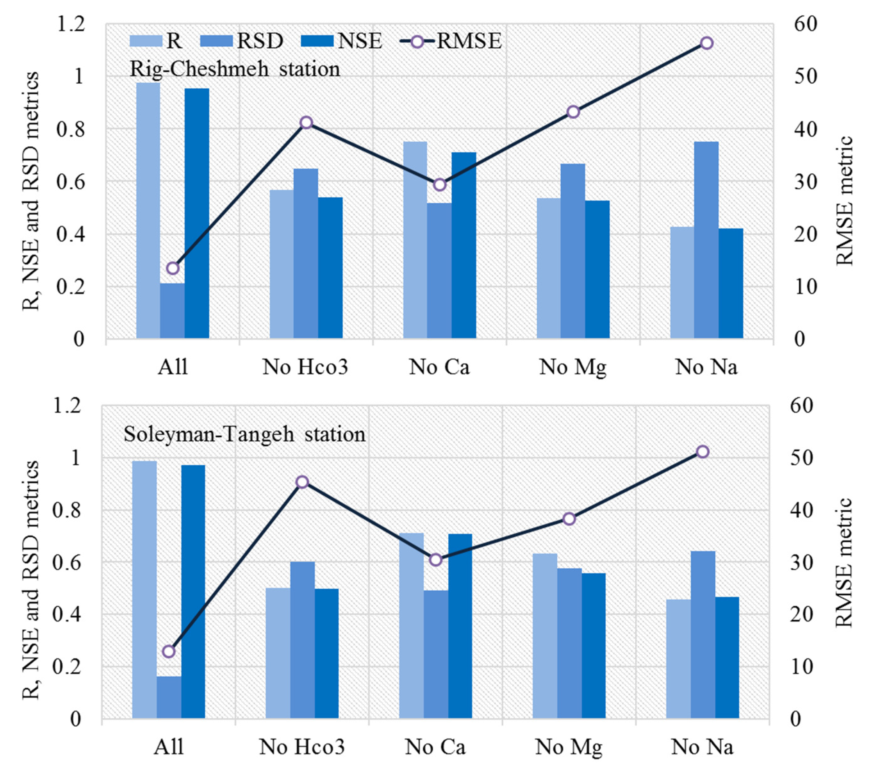
- For further assessment, to compare the results of expected and observation event data, an external validation was performed. Besides, a sensitivity analysis was performed to identify the most influential parameters linked to TDS variations in the Tajan river basin.
2. Materials and Methods
2.1. Artificial Neural Network (ANN)
2.2. Extreme Learning Machine (ELM)
2.3. Adaptive Neuro-Fuzzy Inference System (ANFIS)
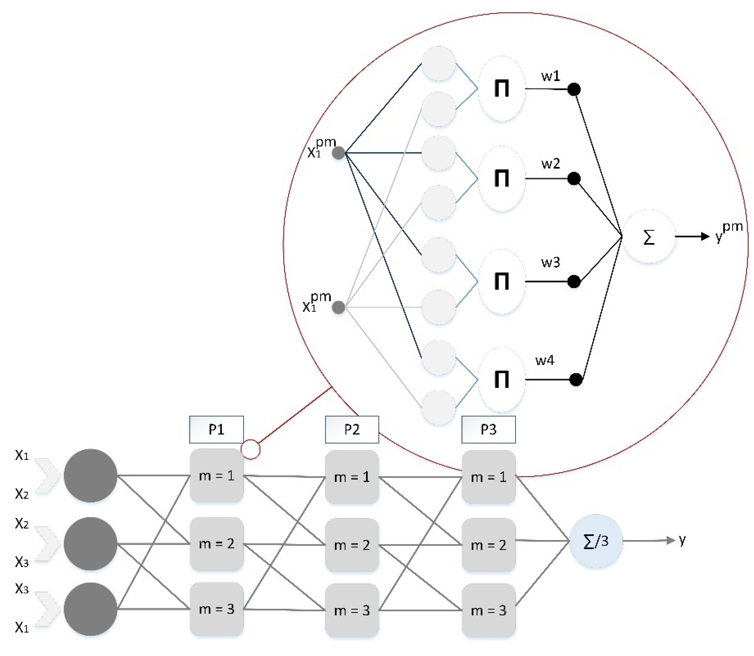
2.4. Group Method of Data Handling (GMDH)
2.5. Particle Swarm Optimization (PSO)
- First, the value of velocity from the prior iteration multiplied by the inertia weight constant, ,
- Second, the difference between the particle’s current position and the best global position , which is also known as social learning, and
- Third, the difference between the particle’s current position and the local best particle’s position up to this point, , which is also known as cognitive learning.
2.6. Grasshopper Optimization Algorithm (GOA)
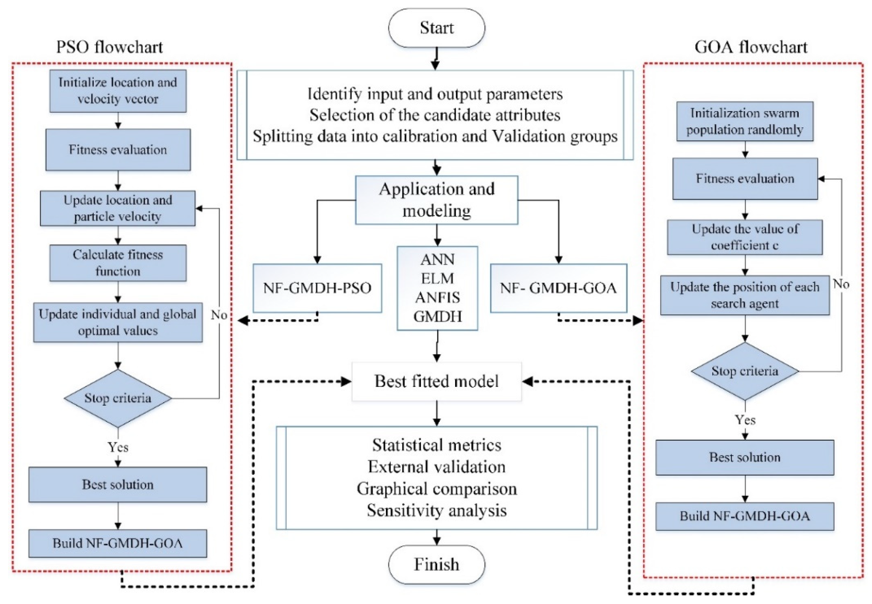
2.7. Development of an Adaptive Fuzzy-GMDH Using PSO/GOA
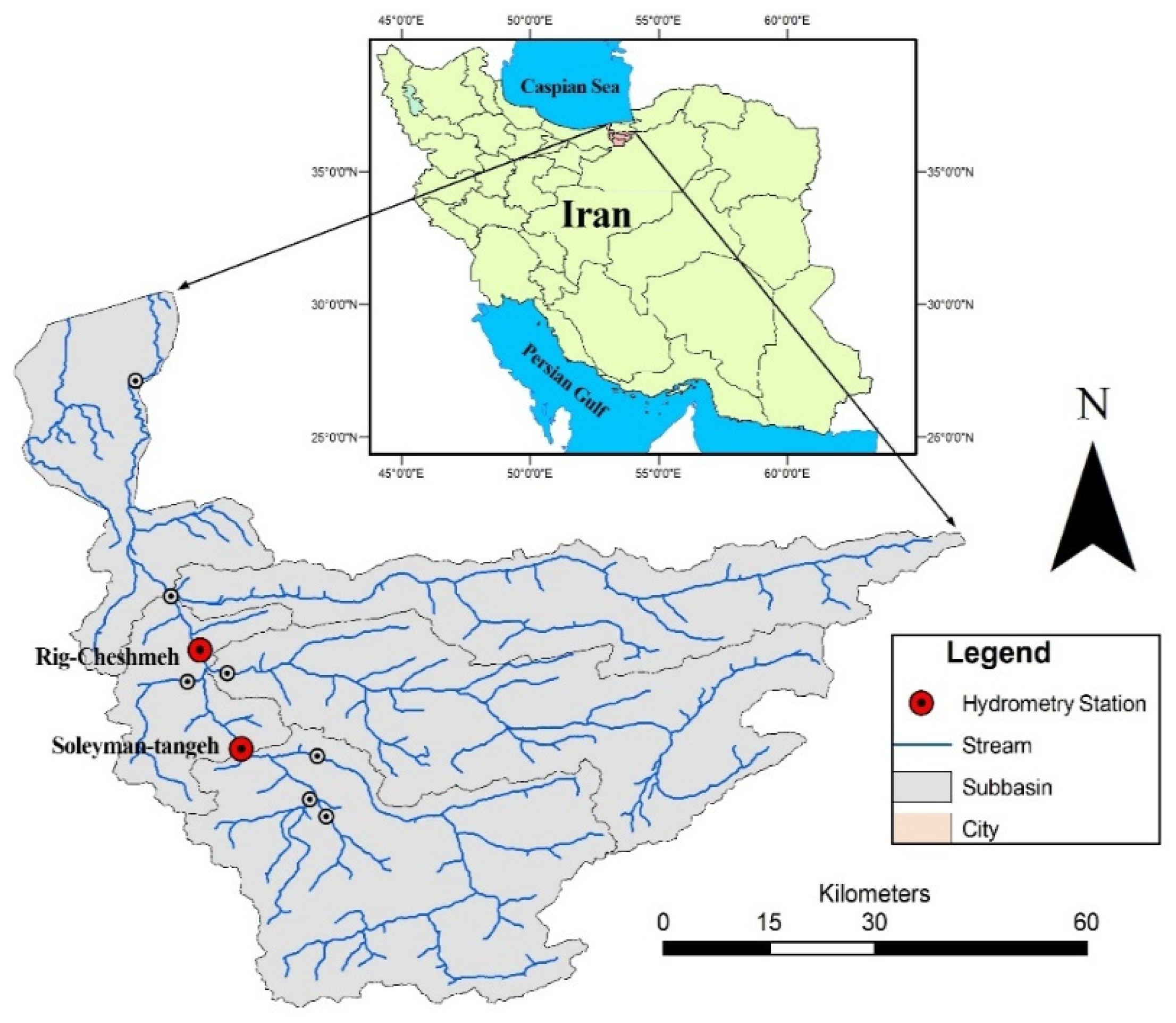
2.8. Case Study Description
2.9. Model Performance Criteria
3. Results and Discussion
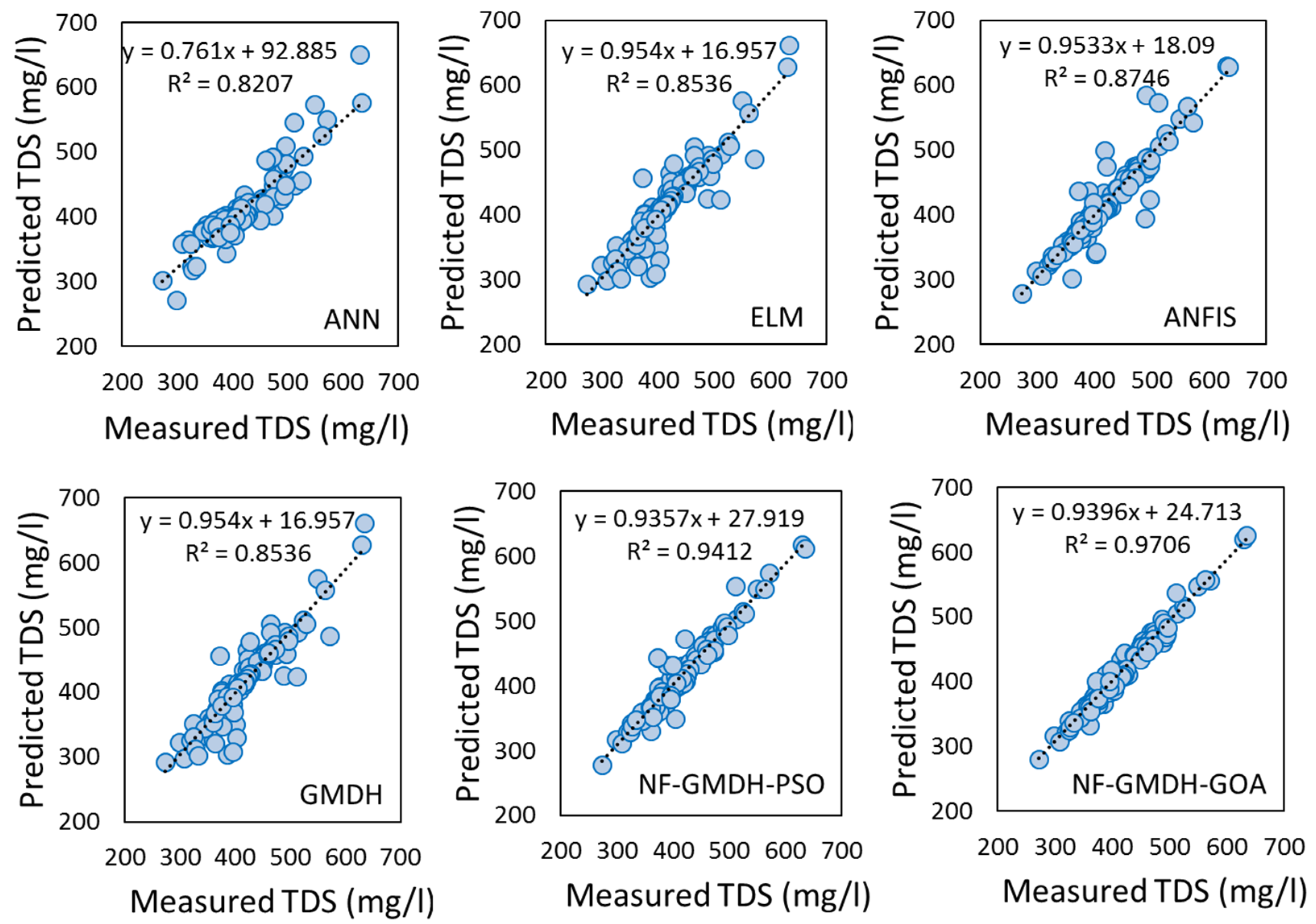
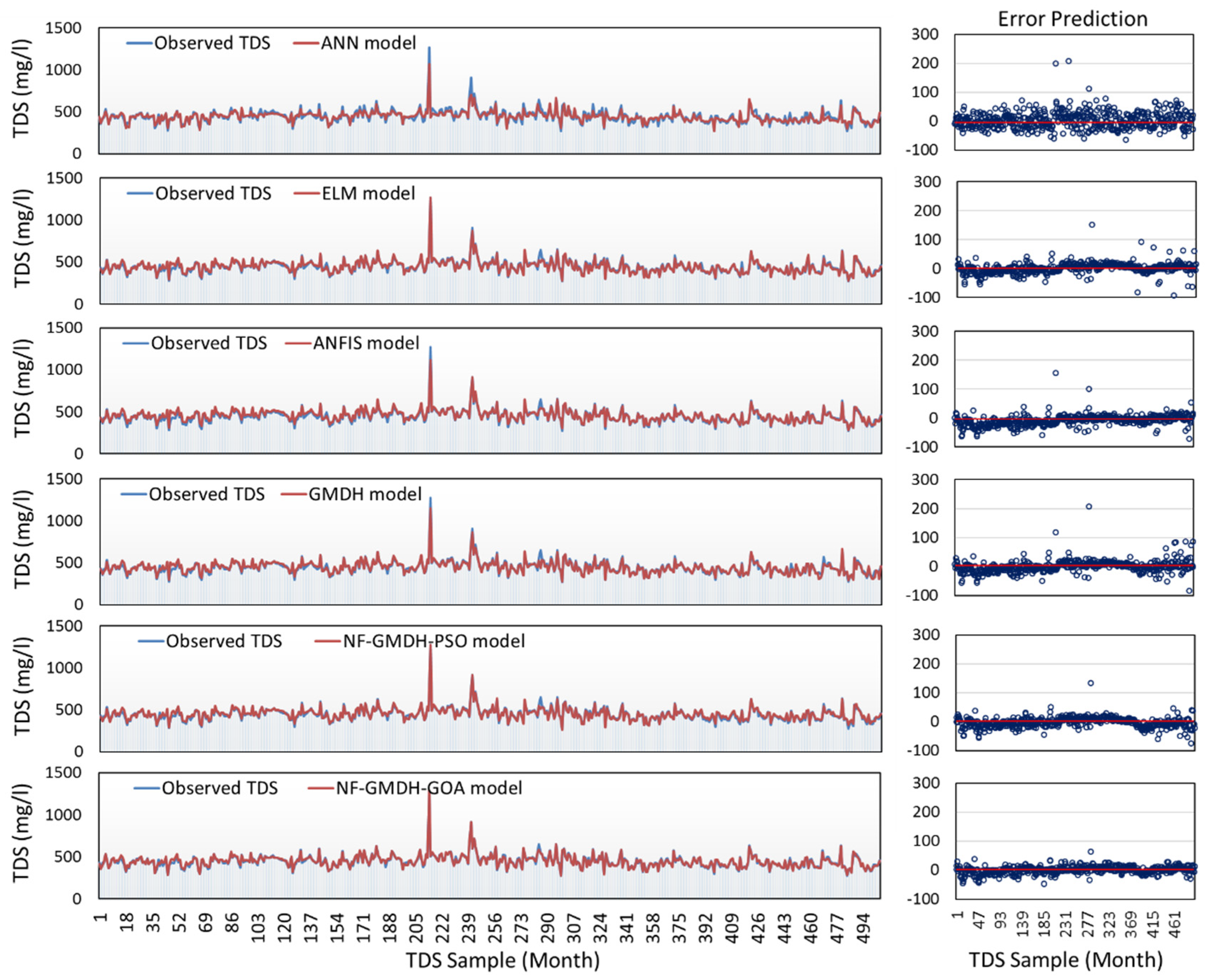
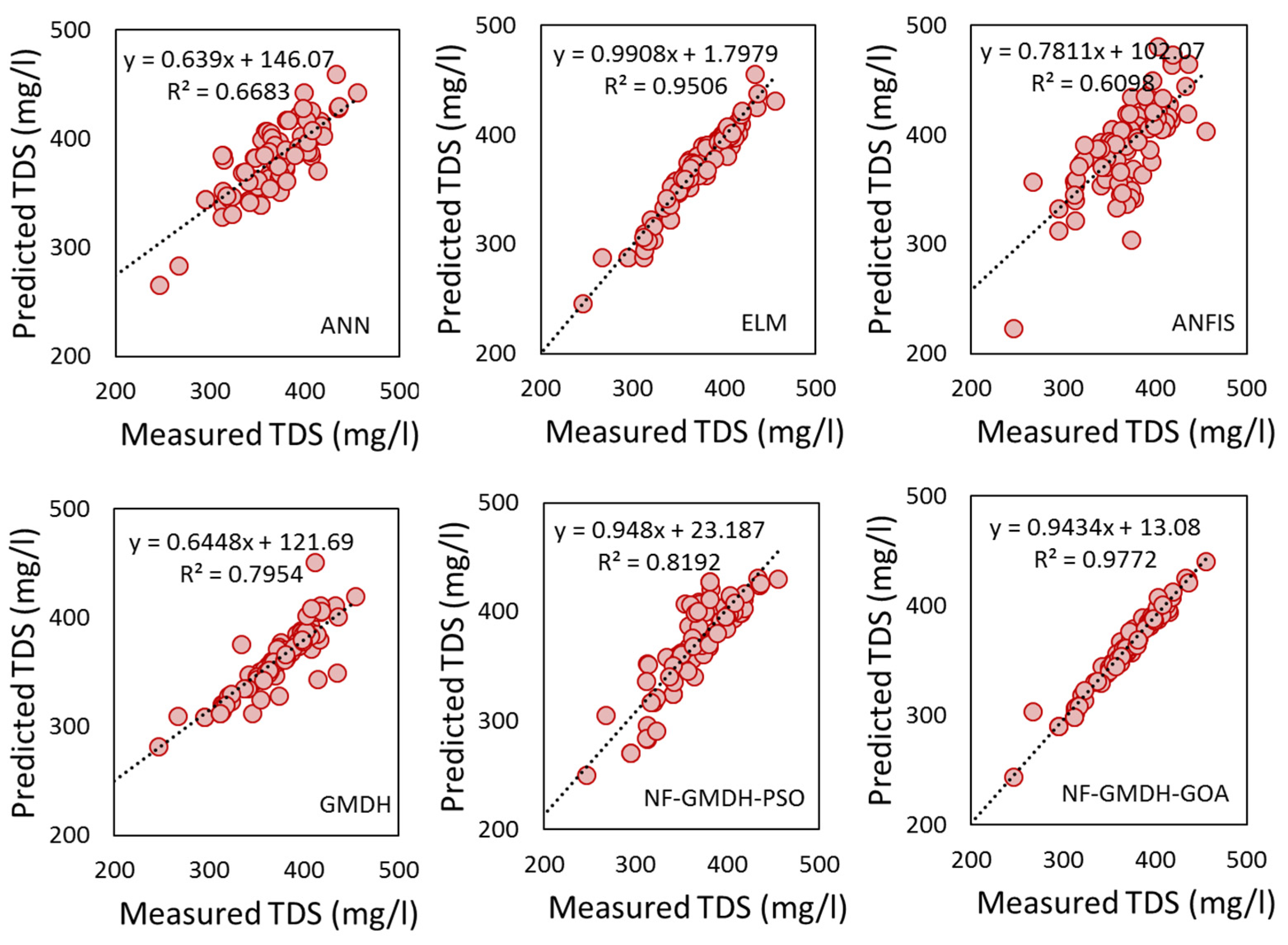
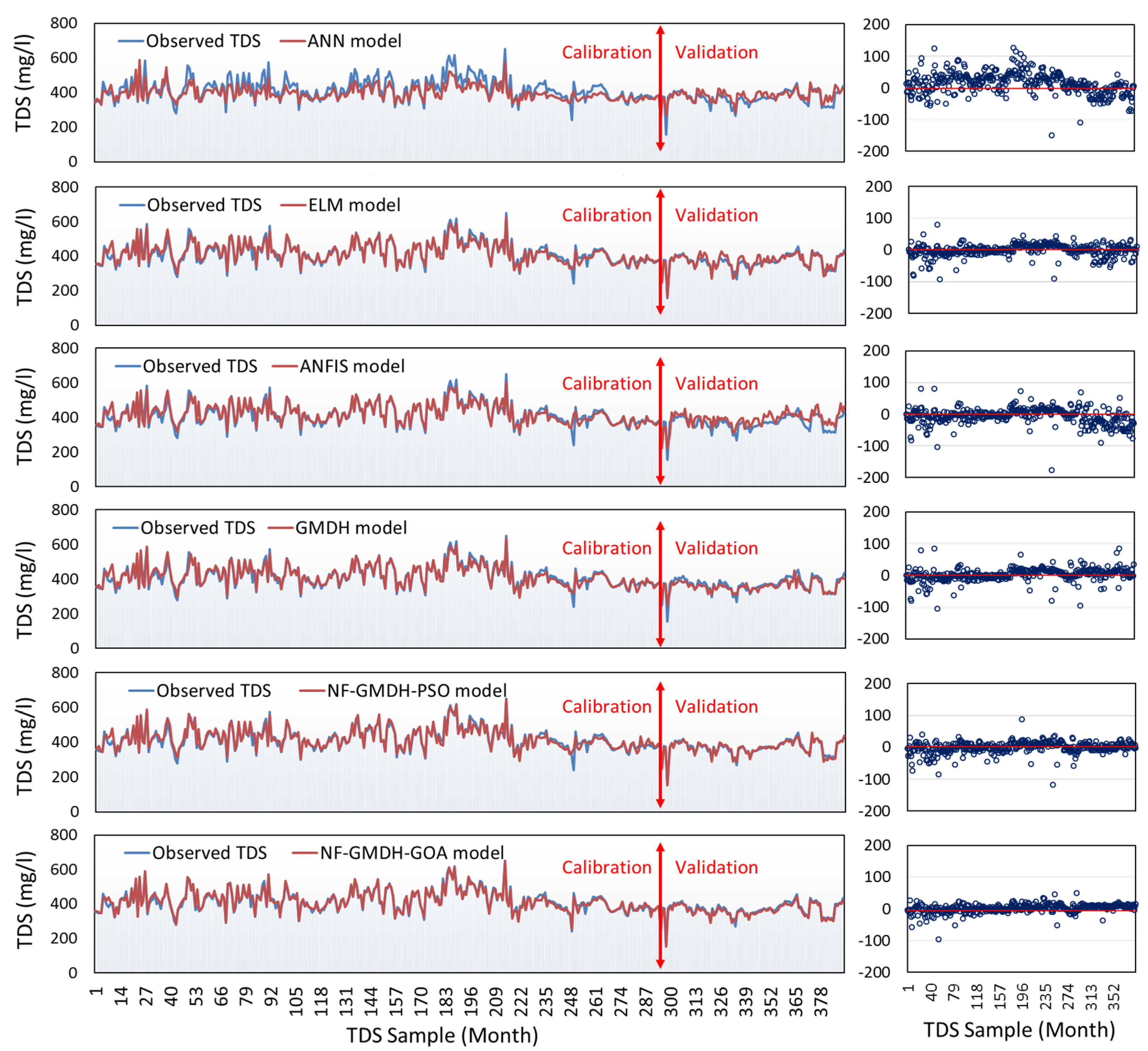
3.1. Performance Results of Standalone and Hybrid Models
3.1.1. The Case Study of Rig-Cheshmeh Station
3.1.2. The Case Study of Soleyman-Tangeh Station
3.2. Further Analysis and Discussion
4. Concluding Remarks
Author Contributions
Funding
Institutional Review Board Statement
Informed Consent Statement
Data Availability Statement
Acknowledgments
Conflicts of Interest
References
- Ahmed, A.N.; Othman, F.B.; Afan, H.A.; Ibrahim, R.K.; Fai, C.M.; Hossain, M.S.; Ehteram, M.; Elshafie, A. Machine Learning Methods for Better Water Quality Prediction. J. Hydrol. 2019, 578, 124084. [Google Scholar] [CrossRef]
- Miranda, J.; Krishnakumar, G. Microalgal Diversity in Relation to the Physicochemical Parameters of Some Industrial Sites in Mangalore, South India. Environ. Monit. Assess. 2015, 187, 664. [Google Scholar] [CrossRef] [PubMed]
- Sibanda, T.; Chigor, V.N.; Koba, S.; Obi, C.L.; Okoh, A.I. Characterisation of the Physicochemical Qualities of a Typical Rural-Based River: Ecological and Public Health Implications. Int. J. Environ. Sci. Technol. 2014, 11, 1771–1780. [Google Scholar] [CrossRef]
- Jonnalagadda, S.B.; Mhere, G. Water Quality of the Odzi River in the Eastern Highlands of Zimbabwe. Water Res. 2001, 35, 2371–2376. [Google Scholar] [CrossRef] [PubMed]
- Kina, C.; Turk, K.; Atalay, E.; Donmez, I.; Tanyildizi, H. Comparison of Extreme Learning Machine and Deep Learning Model in the Estimation of the Fresh Properties of Hybrid Fiber-Reinforced SCC. Neural Comput. Appl. 2021, 33, 11641–11659. [Google Scholar] [CrossRef]
- Rezaie-Balf, M.; Kisi, O. New Formulation for Forecasting Streamflow: Evolutionary Polynomial Regression vs. Extreme Learning Machine. Hydrol. Res. 2018, 49, 939–953. [Google Scholar] [CrossRef]
- Dehghani, M.; Seifi, A.; Riahi-Madvar, H. Novel Forecasting Models for Immediate-Short-Term to Long-Term Influent Flow Prediction by Combining ANFIS and Grey Wolf Optimization. J. Hydrol. 2019, 576, 698–725. [Google Scholar] [CrossRef]
- Vakhshouri, B.; Nejadi, S. Prediction of Compressive Strength of Self-Compacting Concrete by ANFIS Models. Neurocomputing 2018, 280, 13–22. [Google Scholar] [CrossRef]
- Najafzadeh, M.; Rezaie Balf, M.; Rashedi, E. Prediction of Maximum Scour Depth around Piers with Debris Accumulation Using EPR, MT, and GEP Models. J. Hydroinform. 2016, 18, 867–884. [Google Scholar] [CrossRef]
- Sattar, A.M.A.; Gharabaghi, B. Gene Expression Models for Prediction of Longitudinal Dispersion Coefficient in Streams. J. Hydrol. 2015, 524, 587–596. [Google Scholar] [CrossRef]
- Raghavendra, S.; Deka, P.C. Support Vector Machine Applications in the Field of Hydrology: A Review. Appl. Soft Comput. J. 2014, 19, 372–386. [Google Scholar] [CrossRef]
- Barman, M.; Choudhury, N.B.D.; Sutradhar, S. A Regional Hybrid GOA-SVM Model Based on Similar Day Approach for Short-Term Load Forecasting in Assam, India. Energy 2018, 145, 710–720. [Google Scholar] [CrossRef]
- Ghaemi, A.; Rezaie-Balf, M.; Adamowski, J.; Kisi, O.; Quilty, J. On the Applicability of Maximum Overlap Discrete Wavelet Transform Integrated with MARS and M5 Model Tree for Monthly Pan Evaporation Prediction. Agric. For. Meteorol. 2019, 278, 107647. [Google Scholar] [CrossRef]
- Ehteram, M.; Ahmed, A.N.; Latif, S.D.; Huang, Y.F.; Alizamir, M.; Kisi, O.; Mert, C.; El-Shafie, A. Design of a Hybrid ANN Multi-Objective Whale Algorithm for Suspended Sediment Load Prediction. Environ. Sci. Pollut. Res. 2021, 28, 1596–1611. [Google Scholar] [CrossRef] [PubMed]
- Niu, W.; Feng, Z.; Chen, Y.; Zhang, H.; Cheng, C. Annual Streamflow Time Series Prediction Using Extreme Learning Machine Based on Gravitational Search Algorithm and Variational Mode Decomposition. J. Hydrol. Eng. 2020, 25, 4020008. [Google Scholar] [CrossRef]
- Jahanara, A.-A.; Khodashenas, S.R. Prediction of Ground Water Table Using NF-GMDH Based Evolutionary Algorithms. KSCE J. Civ. Eng. 2019, 23, 5235–5243. [Google Scholar] [CrossRef]
- Javdanian, H.; Heidari, A.; Kamgar, R. Energy-Based Estimation of Soil Liquefaction Potential Using GMDH Algorithm. Iran. J. Sci. Technol. Trans. Civ. Eng. 2017, 41, 283–295. [Google Scholar] [CrossRef]
- Abudu, S.; King, J.P.; Sheng, Z. Comparison of the Performance of Statistical Models in Forecasting Monthly Total Dissolved Solids in the Rio Grande 1. JAWRA J. Am. Water Resour. Assoc. 2012, 48, 10–23. [Google Scholar] [CrossRef]
- Khaki, M.; Yusoff, I.; Islami, N. Application of the Artificial Neural Network and Neuro-Fuzzy System for Assessment of Groundwater Quality. CLEAN Soil Air Water 2015, 43, 551–560. [Google Scholar] [CrossRef]
- Asadollahfardi, G.; Zangooi, H.; Asadi, M.; Tayebi Jebeli, M.; Meshkat-Dini, M.; Roohani, N. Comparison of Box-Jenkins Time Series and ANN in Predicting Total Dissolved Solid at the Zāyandé-Rūd River, Iran. J. Water Supply Res. Technol. 2018, 67, 673–684. [Google Scholar] [CrossRef]
- Mustafa, A.S. Artificial Neural Networks Modeling of Total Dissolved Solid in the Selected Locations on Tigris River, Iraq. J. Eng. 2015, 21, 162–179. [Google Scholar]
- Pan, C.; Ng, K.T.W.; Fallah, B.; Richter, A. Evaluation of the Bias and Precision of Regression Techniques and Machine Learning Approaches in Total Dissolved Solids Modeling of an Urban Aquifer. Environ. Sci. Pollut. Res. 2019, 26, 1821–1833. [Google Scholar] [CrossRef]
- Sun, K.; Rajabtabar, M.; Samadi, S.; Rezaie-Balf, M.; Ghaemi, A.; Band, S.S.; Mosavi, A. An Integrated Machine Learning, Noise Suppression, and Population-Based Algorithm to Improve Total Dissolved Solids Prediction. Eng. Appl. Comput. Fluid Mech. 2021, 15, 251–271. [Google Scholar] [CrossRef]
- Zadeh, L.A.; Klir, G.J.; Yuan, B. Fuzzy Sets, Fuzzy Logic, and Fuzzy Systems: Selected Papers; World Scientific: Singapore, 1996; Volume 6. [Google Scholar]
- Tsipouras, M.G.; Exarchos, T.P.; Fotiadis, D.I. A Methodology for Automated Fuzzy Model Generation. Fuzzy Sets Syst. 2008, 159, 3201–3220. [Google Scholar] [CrossRef]
- Wong, W.K.; Guo, Z.X.; Leung, S.Y.S. Optimizing Decision Making in the Apparel Supply Chain Using Artificial Intelligence (AI): From Production to Retail; Elsevier: Amsterdam, The Netherlands, 2013. [Google Scholar]
- Hwang, H.S. Fuzzy GMDH-Type Neural Network Model and Its Application to Forecasting of Mobile Communication. Comput. Ind. Eng. 2006, 50, 450–457. [Google Scholar] [CrossRef]
- Lima, N.N.M.; Linan, L.Z.; Melo, D.N.C.; Manenti, F.; Maciel Filho, R.; Embiruçu, M.; Maciel, M.R.W. Nonlinear Fuzzy Identification of Batch Polymerization Processes. In Computer Aided Chemical Engineering; Elsevier: Amsterdam, The Netherlands, 2015; Volume 37, pp. 599–604. [Google Scholar]
- Zhao, X.; Zhang, Y.; Ning, Q.; Zhang, H.; Ji, J.; Yin, M. Identifying N 6-Methyladenosine Sites Using Extreme Gradient Boosting System Optimized by Particle Swarm Optimizer. J. Theor. Biol. 2019, 467, 39–47. [Google Scholar] [CrossRef]
- Jahandideh-Tehrani, M.; Jenkins, G.; Helfer, F. A Comparison of Particle Swarm Optimization and Genetic Algorithm for Daily Rainfall-Runoff Modelling: A Case Study for Southeast Queensland, Australia. Optim. Eng. 2021, 22, 29–50. [Google Scholar] [CrossRef]
- Dehghani, M.; Riahi-Madvar, H.; Hooshyaripor, F.; Mosavi, A.; Shamshirband, S.; Zavadskas, E.K.; Chau, K. Prediction of Hydropower Generation Using Grey Wolf Optimization Adaptive Neuro-Fuzzy Inference System. Energies 2019, 12, 289. [Google Scholar] [CrossRef]
- Liu, D.; Li, M.; Ji, Y.; Fu, Q.; Li, M.; Faiz, M.A.; Ali, S.; Li, T.; Cui, S.; Khan, M.I. Spatial-Temporal Characteristics Analysis of Water Resource System Resilience in Irrigation Areas Based on a Support Vector Machine Model Optimized by the Modified Gray Wolf Algorithm. J. Hydrol. 2021, 597, 125758. [Google Scholar] [CrossRef]
- Ghaemi, A.; Zhian, T.; Pirzadeh, B.; Hashemi Monfared, S.; Mosavi, A. Reliability-Based Design and Implementation of Crow Search Algorithm for Longitudinal Dispersion Coefficient Estimation in Rivers. Environ. Sci. Pollut. Res. 2021, 28, 35971–35990. [Google Scholar] [CrossRef]
- Mittal, H.; Tripathi, A.; Pandey, A.C.; Pal, R. Gravitational Search Algorithm: A Comprehensive Analysis of Recent Variants. Multimed. Tools Appl. 2021, 80, 7581–7608. [Google Scholar] [CrossRef]
- Duman, S.; Güvenç, U.; Sönmez, Y.; Yörükeren, N. Optimal Power Flow Using Gravitational Search Algorithm. Energy Convers. Manag. 2012, 59, 86–95. [Google Scholar] [CrossRef]
- Tikhamarine, Y.; Malik, A.; Pandey, K.; Sammen, S.S.; Souag-Gamane, D.; Heddam, S.; Kisi, O. Monthly Evapotranspiration Estimation Using Optimal Climatic Parameters: Efficacy of Hybrid Support Vector Regression Integrated with Whale Optimization Algorithm. Environ. Monit. Assess. 2020, 192, 696. [Google Scholar] [CrossRef]
- Pang, Z.; Niu, F.; O’Neill, Z. Solar Radiation Prediction Using Recurrent Neural Network and Artificial Neural Network: A Case Study with Comparisons. Renew. Energy 2020, 156, 279–289. [Google Scholar] [CrossRef]
- Janizadeh, S.; Vafakhah, M. Flood Hydrograph Modeling Using Artificial Neural Network and Adaptive Neuro-Fuzzy Inference System Based on Rainfall Components. Arab. J. Geosci. 2021, 14, 344. [Google Scholar] [CrossRef]
- Elsheikh, A.H.; Sharshir, S.W.; Abd Elaziz, M.; Kabeel, A.E.; Guilan, W.; Haiou, Z. Modeling of Solar Energy Systems Using Artificial Neural Network: A Comprehensive Review. Sol. Energy 2019, 180, 622–639. [Google Scholar] [CrossRef]
- Huang, G.-B.; Zhu, Q.-Y.; Siew, C.-K. Extreme Learning Machine: Theory and Applications. Neurocomputing 2006, 70, 489–501. [Google Scholar] [CrossRef]
- Yaseen, Z.M.; Sulaiman, S.O.; Deo, R.C.; Chau, K.-W. An Enhanced Extreme Learning Machine Model for River Flow Forecasting: State-of-the-Art, Practical Applications in Water Resource Engineering Area and Future Research Direction. J. Hydrol. 2019, 569, 387–408. [Google Scholar] [CrossRef]
- Seo, Y.; Kwon, S.; Choi, Y. Short-Term Water Demand Forecasting Model Combining Variational Mode Decomposition and Extreme Learning Machine. Hydrology 2018, 5, 54. [Google Scholar] [CrossRef]
- Li, X.; Sha, J.; Wang, Z.-L. Comparison of Daily Streamflow Forecasts Using Extreme Learning Machines and the Random Forest Method. Hydrol. Sci. J. 2019, 64, 1857–1866. [Google Scholar] [CrossRef]
- Jang, J.-S. ANFIS: Adaptive-Network-Based Fuzzy Inference System. IEEE Trans. Syst. Man. Cybern. 1993, 23, 665–685. [Google Scholar] [CrossRef]
- Hong, H.; Panahi, M.; Shirzadi, A.; Ma, T.; Liu, J.; Zhu, A.-X.; Chen, W.; Kougias, I.; Kazakis, N. Flood Susceptibility Assessment in Hengfeng Area Coupling Adaptive Neuro-Fuzzy Inference System with Genetic Algorithm and Differential Evolution. Sci. Total Environ. 2018, 621, 1124–1141. [Google Scholar] [CrossRef]
- Azad, A.; Manoochehri, M.; Kashi, H.; Farzin, S.; Karami, H.; Nourani, V.; Shiri, J. Comparative Evaluation of Intelligent Algorithms to Improve Adaptive Neuro-Fuzzy Inference System Performance in Precipitation Modelling. J. Hydrol. 2019, 571, 214–224. [Google Scholar] [CrossRef]
- Zhu, S.; Hadzima-Nyarko, M.; Bonacci, O. Application of Machine Learning Models in Hydrology: Case Study of River Temperature Forecasting in the Drava River Using Coupled Wavelet Analysis and Adaptive Neuro-Fuzzy Inference Systems Model. In Basics of Computational Geophysics; Elsevier: Amsterdam, The Netherlands, 2021; pp. 399–411. [Google Scholar]
- Zaji, A.H.; Bonakdari, H.; Gharabaghi, B. Reservoir Water Level Forecasting Using Group Method of Data Handling. Acta Geophys. 2018, 66, 717–730. [Google Scholar] [CrossRef]
- Jiang, Y.; Liu, S.; Peng, L.; Zhao, N. A Novel Wind Speed Prediction Method Based on Robust Local Mean Decomposition, Group Method of Data Handling and Conditional Kernel Density Estimation. Energy Convers. Manag. 2019, 200, 112099. [Google Scholar] [CrossRef]
- Moosavi, V.; Talebi, A.; Hadian, M.R. Development of a Hybrid Wavelet Packet-Group Method of Data Handling (WPGMDH) Model for Runoff Forecasting. Water Resour. Manag. 2017, 31, 43–59. [Google Scholar] [CrossRef]
- Pattanaik, M.L.; Choudhary, R.; Kumar, B. Prediction of Frictional Characteristics of Bituminous Mixes Using Group Method of Data Handling and Multigene Symbolic Genetic Programming. Eng. Comput. 2020, 36, 1875–1888. [Google Scholar] [CrossRef]
- Ali Ghorbani, M.; Kazempour, R.; Chau, K.-W.; Shamshirband, S.; Taherei Ghazvinei, P. Forecasting Pan Evaporation with an Integrated Artificial Neural Network Quantum-Behaved Particle Swarm Optimization Model: A Case Study in Talesh, Northern Iran. Eng. Appl. Comput. Fluid Mech. 2018, 12, 724–737. [Google Scholar] [CrossRef]
- Nabipour, N.; Dehghani, M.; Mosavi, A.; Shamshirband, S. Short-Term Hydrological Drought Forecasting Based on Different Nature-Inspired Optimization Algorithms Hybridized with Artificial Neural Networks. IEEE Access 2020, 8, 15210–15222. [Google Scholar] [CrossRef]
- Mirjalili, S.Z.; Mirjalili, S.; Saremi, S.; Faris, H.; Aljarah, I. Grasshopper Optimization Algorithm for Multi-Objective Optimization Problems. Appl. Intell. 2018, 48, 805–820. [Google Scholar] [CrossRef]
- Zeynali, M.J.; Shahidi, A. Performance Assessment of Grasshopper Optimization Algorithm for Optimizing Coefficients of Sediment Rating Curve. AUT J. Civ. Eng. 2018, 2, 39–48. [Google Scholar]
- Aljarah, I.; Al-Zoubi, A.; Faris, H.; Hassonah, M.A.; Mirjalili, S.; Saadeh, H. Simultaneous Feature Selection and Support Vector Machine Optimization Using the Grasshopper Optimization Algorithm. Cognit. Comput. 2018, 10, 478–495. [Google Scholar] [CrossRef]
- Najafzadeh, M.; Bonakdari, H. Application of a Neuro-Fuzzy GMDH Model for Predicting the Velocity at Limit of Deposition in Storm Sewers. J. Pipeline Syst. Eng. Pract. 2017, 8, 6016003. [Google Scholar] [CrossRef]
- Harandizadeh, H.; Toufigh, V. Application of Developed New Artificial Intelligence Approaches in Civil Engineering for Ultimate Pile Bearing Capacity Prediction in Soil Based on Experimental Datasets. Iran. J. Sci. Technol. Trans. Civ. Eng. 2020, 44, 545–559. [Google Scholar] [CrossRef]
- Rezaie-Balf, M. Multivariate Adaptive Regression Splines Model for Prediction of Local Scour Depth Downstream of an Apron under 2D Horizontal Jets. Iran. J. Sci. Technol. Trans. Civ. Eng. 2019, 43, 103–115. [Google Scholar] [CrossRef]


| Algorithm | Parameters | Value |
|---|---|---|
| PSO | Acceleration constant (C1 and C2) | 2 |
| Inertia Wmax | 0.9 | |
| Inertia Wmin | 0.4 | |
| Number of particles | 50 | |
| GOA | Seeking memory pool | 5 |
| Counts of dimension to change | 0.8 | |
| Seeking rang of the selected dimension | 0.2 | |
| Mutative ratio | 0.9 |
| Variables | Indices | Rig-Cheshmeh | Soleyman-Tangeh |
|---|---|---|---|
| HCO3 (mg/L) | Min | 1.6 | 1.2 |
| Mean | 3.88 | 1.2 | |
| Max | 12.2 | 0.5 | |
| Std | 0.89 | 0.08 | |
| Variation | 0.79 | 156 | |
| Ca (mg/L) | Min | 1.1 | 3.84 |
| Mean | 3.16 | 3.41 | |
| Max | 7.5 | 2.07 | |
| Std | 0.68 | 0.87 | |
| Variation | 0.46 | 408.87 | |
| Mg (mg/L) | Min | 0.1 | 7.7 |
| Mean | 2.17 | 6.3 | |
| Max | 6 | 4.5 | |
| Std | 0.69 | 2.94 | |
| Variation | 0.48 | 650 | |
| Na (mg/L) | Min | 0.2 | 0.91 |
| Mean | 1.54 | 0.66 | |
| Max | 6.5 | 0.68 | |
| Std | 0.75 | 0.42 | |
| Variation | 0.57 | 63.1 | |
| TDS (mg/L) | Min | 271 | 0.83 |
| Mean | 446.49 | 0.44 | |
| Max | 1270 | 0.46 | |
| Std | 78.7 | 0.18 | |
| Variation | 6194.38 | 3981.8 |
| ANN | ELM | ANFIS | GMDH | NF-GMDH-PSO | NF-GMDH-GOA | |
|---|---|---|---|---|---|---|
| Calibration | ||||||
| R | 0.947 | 0.975 | 0.973 | 0.968 | 0.980 | 0.986 |
| RMSE (mg/L) | 29.991 | 18.053 | 22.222 | 20.784 | 16.099 | 13.478 |
| RSD | 0.369 | 0.222 | 0.273 | 0.256 | 0.198 | 0.166 |
| NSE | 0.864 | 0.951 | 0.925 | 0.934 | 0.961 | 0.972 |
| Validation | ||||||
| R | 0.906 | 0.935 | 0.970 | 0.924 | 0.962 | 0.985 |
| RMSE (mg/L) | 27.178 | 22.439 | 14.975 | 24.579 | 20.564 | 10.744 |
| RSD | 0.440 | 0.363 | 0.242 | 0.398 | 0.333 | 0.174 |
| NSE | 0.805 | 0.867 | 0.941 | 0.840 | 0.888 | 0.970 |
| ANN | ELM | ANFIS | GMDH | NF-GMDH-PSO | NF-GMDH-GOA | |
|---|---|---|---|---|---|---|
| Calibration | ||||||
| R | 0.891 | 0.950 | 0.932 | 0.948 | 0.948 | 0.973 |
| RMSE (mg/L) | 40.295 | 19.538 | 22.807 | 19.938 | 20.107 | 14.376 |
| RSD | 0.640 | 0.310 | 0.362 | 0.317 | 0.320 | 0.228 |
| NSE | 0.589 | 0.903 | 0.868 | 0.899 | 0.898 | 0.948 |
| Validation | ||||||
| R | 0.817 | 0.905 | 0.781 | 0.892 | 0.975 | 0.989 |
| RMSE (mg/L) | 27.823 | 19.378 | 35.364 | 22.254 | 10.113 | 9.687 |
| RSD | 0.655 | 0.456 | 0.833 | 0.524 | 0.238 | 0.223 |
| NSE | 0.567 | 0.790 | 0.300 | 0.723 | 0.942 | 0.948 |
| Metrics | ANN | ELM | ANFIS | GMDH | NF-GMDH-PSO | NF-GMDG-GOA |
|---|---|---|---|---|---|---|
| Rig-Cheshmeh station | ||||||
| R (R > 0.8) | 0.906 | 0.935 | 0.97 | 0.924 | 0.962 | 0.985 |
| K (0.85 < K < 1.15) | 1.017 | 1.001 | 0.997 | 1.003 | 0.975 | 1.002 |
| K′ (0.85 < K′ < 1.15) | 0.979 | 0.996 | 1.001 | 0.994 | 1.024 | 0.998 |
| m (m < 0.1) | −0.202 | −0.143 | −0.062 | −0.171 | −0.047 | −0.03 |
| n (n < 0.1) | −0.185 | −0.142 | −0.062 | −0.17 | −0.042 | −0.03 |
| Rm (Rm > 0.5) | 0.48 | 0.565 | 0.714 | 0.527 | 0.732 | 0.804 |
| Soleyman-Tangeh station | ||||||
| R (R > 0.8) | 0.817 | 0.905 | 0.781 | 0.892 | 0.975 | 0.989 |
| K (0.85 < K < 1.15) | 0.965 | 0.987 | 0.943 | 1.026 | 1.004 | 1.022 |
| K′ (0.85 < K′ < 1.15) | 1.031 | 0.101 | 0.055 | 0.972 | 0.996 | 0.979 |
| m (m < 0.1) | −0.36 | −0.206 | −0.226 | −0.191 | −0.051 | 0.013 |
| n (n < 0.1) | −0.301 | −0.212 | −0.211 | −0.116 | −0.051 | 0.015 |
| Rm (Rm > 0.5) | 0.341 | 0.483 | 0.384 | 0.485 | 0.741 | 0.866 |
| Number | Pairwise Comparison | Z | p (<0.05) | Significance |
|---|---|---|---|---|
| 1 | NF-GMDH-GOA vs. ANN | −4.496 | 0.003 | Yes |
| 2 | NF-GMDH-GOA vs. ELM | −5.621 | 0.001 | Yes |
| 3 | NF-GMDH-GOA vs. ANFIS | −7.255 | 0.001 | Yes |
| 4 | NF-GMDH-GOA vs. GMDH | −7.158 | 0.002 | Yes |
| 5 | NF-GMDH-GOA vs. NF-GMDH-PSO | −8.157 | 0.001 | Yes |
Disclaimer/Publisher’s Note: The statements, opinions and data contained in all publications are solely those of the individual author(s) and contributor(s) and not of MDPI and/or the editor(s). MDPI and/or the editor(s) disclaim responsibility for any injury to people or property resulting from any ideas, methods, instructions or products referred to in the content. |
© 2023 by the authors. Licensee MDPI, Basel, Switzerland. This article is an open access article distributed under the terms and conditions of the Creative Commons Attribution (CC BY) license (https://creativecommons.org/licenses/by/4.0/).
Share and Cite
Hijji, M.; Chen, T.-C.; Ayaz, M.; Abosinnee, A.S.; Muda, I.; Razoumny, Y.; Hatamiafkoueieh, J. Optimization of State of the Art Fuzzy-Based Machine Learning Techniques for Total Dissolved Solids Prediction. Sustainability 2023, 15, 7016. https://doi.org/10.3390/su15087016
Hijji M, Chen T-C, Ayaz M, Abosinnee AS, Muda I, Razoumny Y, Hatamiafkoueieh J. Optimization of State of the Art Fuzzy-Based Machine Learning Techniques for Total Dissolved Solids Prediction. Sustainability. 2023; 15(8):7016. https://doi.org/10.3390/su15087016
Chicago/Turabian StyleHijji, Mohammad, Tzu-Chia Chen, Muhammad Ayaz, Ali S. Abosinnee, Iskandar Muda, Yury Razoumny, and Javad Hatamiafkoueieh. 2023. "Optimization of State of the Art Fuzzy-Based Machine Learning Techniques for Total Dissolved Solids Prediction" Sustainability 15, no. 8: 7016. https://doi.org/10.3390/su15087016
APA StyleHijji, M., Chen, T.-C., Ayaz, M., Abosinnee, A. S., Muda, I., Razoumny, Y., & Hatamiafkoueieh, J. (2023). Optimization of State of the Art Fuzzy-Based Machine Learning Techniques for Total Dissolved Solids Prediction. Sustainability, 15(8), 7016. https://doi.org/10.3390/su15087016