Article

An Analytical Solution for Unsteady Aerodynamic Forces on Streamlined Box Girders with Coupled Vibration

1
Department of Bridge Engineering, Southwest Jiaotong University, Chengdu 610031, China
2
China 19th Metallurgical Corporation, Chengdu 610031, China
*
Author to whom correspondence should be addressed.
Sustainability 2023, 15(9), 7312; https://doi.org/10.3390/su15097312
Submission received: 6 March 2023 / Revised: 18 April 2023 / Accepted: 26 April 2023 / Published: 27 April 2023

Abstract

:
This paper is a contribution to analyzing the aerodynamic forces on a streamlined box girder (SBG) with coupled vibration in a potential flow. The key enabling step was to assume that the normal velocity of the airflow at an arbitrary point on the surface of the SBG was equal to the normal velocity of the surface motion. The aerodynamic drag force, lift force, and pitching moment were expressed as functions of the motion state of the SBG and the SBG’s shape-related parameters. To investigate the applicability of this force model, the analytical solution at various angles of attack was compared with a numerical simulation in a viscous flow. The results imply that the amplitude of the analytical lift force and pitching moment agree well with the numerical results under the angles of attack of 0° and ±3°. Furthermore, the analytical drag force effectively predicts the second-order phenomenon resulting from the multiplication of the vertical and torsional vibration velocities. As a consequence, the present analytical solution provides an effective method for analyzing the aerodynamic forces acting on SBGs with coupled vibration.

1. Introduction

The shift towards environmentally friendly and sustainable solutions has become a ubiquitous aspect of modern life. Over the course of several decades, it has played a significant role in shaping the design, construction, and maintenance of bridges. Wind can cause significant vibrations on bridges, including vortex-induced vibration, flutter, and buffet [1,2], which have the potential to damage the bridge’s structure and compromise its long-term sustainability. Therefore, it is crucial to conduct an aerodynamic force study on bridges to ensure their wind resistance safety.
The analysis of unsteady aerodynamic forces and vibrations has been a subject of significant interest in the field of engineering [3,4,5], particularly in the design and analysis of streamlined box girder (SBG) bridges. The increasing demand for long-span bridges makes the bridge structure increasingly sensitive to the wind load [6,7], which can result in remarkable structural vibrations [8,9,10] and even the collapse of the bridge [11]. The potential flow theory can provide a useful framework for understanding the basic principles of fluid flow and the resulting forces on structures. It has been extensively used to design airfoils. However, the application of the potential flow theory to the aerodynamic forces acting on SBGs has not been thoroughly studied. This study proposes an analytical solution for unsteady aerodynamic forces acting on SBGs with coupled vibration in a potential flow and investigates its applicability.
A model coupled via aerodynamic derivatives has long been widely used to describe aerodynamic forces [12,13]. Through flutter derivatives and the motion state of the main girder, the aerodynamic drag force, lift force, and pitching moment can be determined. The flutter derivatives can be obtained by measuring the aerodynamic force at a limited number of wind speeds via the wind tunnel test [14,15,16] and a computational fluid dynamics (CFD) study [17,18,19,20]. The classical Scanlan model is linearized. The frequency of an unsteady force is equal to the coupled vibration frequency. It is not able to explain the high-order unsteady force phenomenon, which was discovered through wind tunnel tests and CFD [21,22]. The common step to consider the high-order component is to add the high-order term in the aerodynamic force model. However, there are few explanations for the generation of high-order components.
The potential flow theory has been widely used in predicting the aerodynamic forces on an airfoil. Von Karman and Sears [23] and Theodorsen [24] presented the general theory of aerodynamic forces on an oscillating thin airfoil. Edwards et al. [25] derived the unsteady aerodynamic loads due to the arbitrary motions of a thin wing. Sun and Wang [26] developed a numerical model for calculating the unsteady flow of an elliptical circulation-control airfoil. Stangfeld et al. [27] compared the aerodynamic loads acting on a relatively thick NACA 0018 airfoil (a symmetric airfoil with a thickness-to-chord ratio of 18% and a maximum thickness located at 30% of the chord length) with pitching and heaving vibrations. Excellent correspondence was found between the experimentally obtained aerodynamic forces and potential theory. Catlett et al. [28] investigated the unsteady pressures and forces on airfoils with an oscillating motion. The unsteady lift forces and pitching moment of the thin airfoils agreed well with the CFD results. In addition, the potential theory was also applied to evaluate the aerodynamic loads on a railway train [29,30] and cylinders [31]. All the aforementioned works indicated the good performance of the potential flow theory in the calculation of aerodynamic forces on various types of structures. However, it is difficult to find research studying the application of the potential flow theory in bridge engineering.
Studying the analytical solution for aerodynamic forces is of great significance in enhancing the sustainability of bridge structures. However, the real flow is too complex to find an explicit expression to calculate the aerodynamic force. Therefore, this paper primarily concentrates on the analytical aerodynamic forces of an SBG with coupled vibration based on the potential flow theory. This solution is expected to offer insights into the underlying aerodynamic principles, paving the way for more precise models of aerodynamic performance in future studies. Meanwhile, the distinction between the aerodynamic forces in a potential flow and a viscous flow was analyzed.
To investigate the unsteady aerodynamic forces on the SBG, the present paper is organized as follows: Section 2 renders the complex potential on the surface of the SBG and in the whole flow domain. The analytical solution of the aerodynamic forces is derived in Section 3. In Section 4, to study the applicability of the potential flow solution in bridge engineering, the analytical solution is compared with the numerical results in a viscous flow. Finally, the conclusions are summarized.

2. Complex Potential

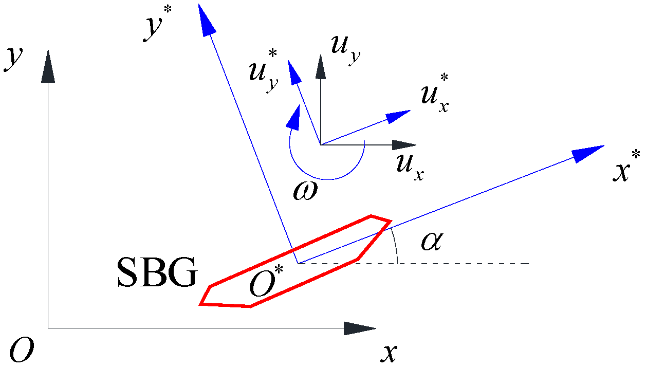
2.1. Stream Function on the Surface of an SBG

The complex potential w(z) is an analytic function in an ideal flow whose real part is the velocity potential ϕ and whose imaginary part is the stream function ψ, as presented in Equation (1), where i is the imaginary unit. Thus, to obtain the aerodynamic force of a moving SBG, it is essential to determine the complex potential of the SBG.
w z = ϕ + i ψ
Assume that an SBG is in an arbitrary coupled vibration of its horizontal velocity ux, vertical velocity uy, and angular velocity ω, as displayed in Figure 1. The coordinate of a point P on the SBG relative to the center of mass of the SBG is (xp, yp); then, the velocity of point P can be expressed as follows:
u p x = u x + ω y p u p y = u y ω x p
Let the angle between the surface of point P and the positive direction of the x-axis be θ; then, the normal velocity upn at point P becomes:
u p n = u x + ω y p sin θ u y ω x p cos θ
According to the geometrical condition, we have:
sin θ = d y d c , cos θ = d x d c
where c is the surface of SBG; dx, dy, and dc denote the infinitesimal increase in x, y, and c.
Since the air cannot penetrate through the surface of the SBG, the normal velocity of the airflow at point P is equal to the normal velocity of the SBG motion at point P. Therefore, the normal velocity upn can be expressed as follows:
u p n = ψ c
Substituting Equations (4) and (5) into Equation (3) leads to:
ψ c = u x + ω y d y d c u y ω x d x d c
where ∂ψ and ∂c represent the partial differentials of ψ and c, respectively. Integrating Equation (6), the stream function ψ can be given as follows:
ψ = u x y u y x + 1 2 ω x 2 + y 2 + C o n s t
where Const means a constant.

2.2. Complex Potential in the Fluid Domain

To obtain the complex potential, we define a function:
f z , z ¯ = u ¯ z + 1 2 i ω z z ¯
in which z = x + iy, u = ux + iuy; z ¯ and u ¯ are complex conjugate of z and u, respectively. Then, the imaginary part of Equation (8) is equal to Equation (7) without the constant term, i.e.,
2 i ψ = f z , z ¯ f ¯ z , z ¯ = u ¯ z u z ¯ + i ω z z ¯
where f ¯ is the complex conjugate of f. Assume that z = f(ζ) is the conformal mapping function from a unit circle in the ζ-plane to the SBG in the z-plane. The point on the edge of the unit circle ζu can be written as:
ζ u = e i θ , ζ ¯ u = e i θ = 1 ζ u
where ζ ¯ u is the complex conjugate of ζ u . Introducing z = f(ζ) and Equation (10) into Equation (9) leads to:
2 i ψ = u ¯ f ζ u u f 1 ζ u + i ω f ζ u f 1 ζ u = B ζ u
in which B(ζu) is the surface function of SBG, expressed by ζu. The complex potential of the unit circle satisfies:
w ζ u w 1 ζ u = 2 i ψ
Therefore, the relationship between the complex potential on the surface of the unit circle and the surface function can be exhibited as:
w ζ u w 1 ζ u = B ζ u
Here, the complex potential on the surface will be extended to the full fluid domain. The surface function can be written as:
B ζ u = B 1 ζ u + B 2 ζ u
where B1(ζu) is the negative exponential term, and B2(ζu) is the non-negative exponential term. Let Equation (14) be divided by 2πi(ζuζ). Integrating both sides of the equation on the surface of the unit circle arrives at:
C B ζ u 2 π i ζ u ζ d ζ u = 1 2 π i C B 1 ζ u ζ u ζ d ζ u + 1 2 π i C B 2 ζ u ζ u ζ d ζ u = 1 2 π i C w ζ u ζ u ζ d ζ u 1 2 π i C w 1 / ζ u ζ u ζ d ζ u
On the basis of the Cauchy integral formula [32]:
1 2 π i C w ζ u ζ u ζ d ζ u = w ζ , 1 2 π i C w 1 / ζ u ζ u ζ d ζ u = 0 1 2 π i C B 1 ζ u ζ u ζ d ζ u = B 1 ζ , 1 2 π i C B 2 ζ u ζ u ζ d ζ u = 0
Then the complex potential of the SBG becomes:
w ζ = B 1 ζ
The conformal mapping from a unit circle in the ζ-plane to the SBG in the z-plane can be expressed in the Laurent series [33] as follows:
z = k = 1 n c k ζ 2 k
in which ck = ak + ibk, ak, and bk and are real coefficients to be determined [34]. Introducing Equation (18) into Equation (11), the surface function of SBG is then determined as:
B ζ = u ¯ k = 1 n c k ζ 2 k u k = 1 n c ¯ k ζ ¯ 2 k + i ω k = 1 n c k ζ 2 k k = 1 n c ¯ k ζ ¯ 2 k
According to Equation (17), the complex potential of the SBG with coupled vibration is the negative exponential term of the surface function. Therefore, the complex potential can be obtained from Equation (19):
w ζ = u ¯ k = 3 n c k ζ 2 k u c ¯ 1 1 ζ + i ω k = 1 n 1 j = k + 1 n c ¯ k c j ζ k j

3. Aerodynamic Forces

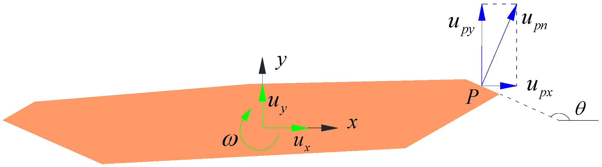
3.1. Pressure Function

Due to the low density of the airflow, the resultant pressure induced by the variation in the relative elevation of the SBG is deemed negligible. This implies that any minute alterations in the SBG’s height are unlikely to exert a noteworthy influence on the ambient airflow, and the associated pressure can therefore be justifiably disregarded. In light of the unsteady Bernoulli equation [35], the pressure equation of the ideal incompressible fluid can be expressed as [28]:
p + ρ ϕ t + 1 2 ρ V 2 = C o n s t t
where p is the aerodynamic pressure; ρ is the air density; ϕ is the potential function; V = u x , u y is the vector of wind velocity; Const(t) means a constant.
To obtain the pressure function, two coordinate systems are established. As shown in Figure 2, x*O*y* is a moving coordinate system that moves with the SBG whose x*-axis is always parallel to the long axis of the SBG. xOy is a static coordinate system. α is the angle between the two coordinate systems. The velocity component is represented by u x * and u y * in the x*O*y* coordinate system and u x and u y in the xOy coordinate system, respectively. Their relationships are then expressed as follows:
u x * = u x cos α + u y sin α , u y * = u x sin α + u y cos α d x * = d x cos α + d y sin α , d y * = d x sin α + d y cos α
The potential function in the x*O*y* coordinate system is defined as ϕ * = ϕ * x * , y * , t *   = u x * d x * + u y * d y * . Introducing Equation (22) into the above formula, it can be found that ϕ * = ϕ , i.e., the potential functions in the two coordinate systems are equal. The partial derivative of ϕ with respect to time t is:
ϕ t = lim Δ t 0 ϕ * x t + Δ t * , y t + Δ t * , t + Δ t ϕ * x t * , y t * , t Δ t
In the x*O*y* coordinate system, the location of x * , y * at time t + Δt can be expressed as:
x t + Δ t * = x t * u x + ω y t * Δ t , y t + Δ t * = y t * u y ω x t * Δ t
Substituting Equation (24) into Equation (23), we arrive:
ϕ t = ϕ * t V 0 * ϕ *
Since
V 0 V ¯ 0 = u x + ω y + i u y ω x u x + ω y + i u y ω x ¯ = u i ω z u ¯ + i ω z ¯
Finally, introducing Equations (25) and (26) into Equation (21), the pressure function p can finally be obtained as follows:
p = ρ ϕ t + 1 2 ρ u i ω z u ¯ + i ω z ¯ 1 2 ρ e i 2 β d w z d z u ¯ + i ω z ¯ 2
where β is the angle between the vector formed by a point in the flow field and the coordinate origin and the x-axis.

3.2. Drag Force and Lift Force

On the basis of the complex variable theory, it is known that d z ¯ = d z e i 2 β . Integrating the pressure function Equation (27) on the surface of the SBG, the aerodynamic force of the SBG can be acquired:
F x i F y = i C p d z ¯ = i C p e i 2 β d z
where Fx is the aerodynamic drag force of SBG, and Fy is the aerodynamic lift force of SBG. Substituting Equation (27) into Equation (28), the complex expression of the aerodynamic force becomes:
F x i F y = 1 2 i ρ C u i ω z u ¯ + i ω z ¯ d z ¯ + 1 2 i ρ C d w z d z 2 d z + 1 2 i ρ C u ¯ + i ω z ¯ 2 d z i ρ C d w z d z u ¯ + i ω z ¯ d z + i ρ C ϕ t d z ¯
To simplify Equation (29), we can define the function f z , z ¯ as:
f x = f z z x + f z ¯ z ¯ x = f z + f z ¯ f y = f z z y + f z ¯ z ¯ y = i f z f z ¯
According to Stokes’ theorem [36], the integral along the surface of SBG can be expressed as an area fraction:
C f d r = S e z × f d S = e z × S f x e x + f y e y d S
where S is the inner region of SBG, and ex, ey, and ez are the unit vectors along the coordinate axis. Considering that ey = ez × ex = iex, dr = exdx + eydy = exdz, Equation (31) becomes:
C f d z = i S f x + i f y d S
Introducing Equation (32) into Equation (30), we have:
C f z , z ¯ d z = 2 i S f z ¯ d S C f z , z ¯ d z ¯ = 2 i S f z d S
Assume that the area of the SBG is A, and zc is the geometric center of the SBG, which can be expressed as z c = 1 A S z d S . Then, in the light of Equation (33), the first and third terms in Equation (29) become:
1 2 i ρ C u i ω z u ¯ + i ω z ¯ d z ¯ = 1 2 i ρ 2 i S i ω u ¯ + i ω z ¯ d S = i ρ ω A u ¯ + i ω z ¯ c 1 2 i ρ C u ¯ + i ω z ¯ 2 d z = 1 2 i ρ 2 i S 2 i ω u ¯ + i ω z ¯ d S = 2 i ρ ω A u ¯ + i ω z ¯ c
According to the definition of the complex potential function, it is known that C ϕ d z ¯ = 1 2 C w d z ¯ + C w ¯ d z ¯ . Thus, the expression of the resultant force of the SBG expressed by the complex potential function can finally be attained as follows:
F x i F y = i ρ ω A u ¯ + i ω z ¯ c + 1 2 i ρ C d w z d z 2 d z i ρ u ¯ C d w z + ρ ω C z ¯ d w z + 1 2 i ρ t C w z d z ¯ + C w ¯ z d z ¯
By substituting Equations (18) and (20) into Equation (35) and then integrating it, the aerodynamic drag force and lift force are represented as follows:
F x = ρ A ω u y + Re F F y = ρ A ω u x Im F
where Re(F) and Im(F) are the real part and imaginary part of F, which is expressed as:
F = ρ ω 2 π i u ¯ k = 3 n 2 k c ¯ k c k + u c 1 c 3 + i ω k = 3 n j = 1 n k + 2 c ¯ k c ¯ j c j + k 2 2 k π ρ u ¯ t c 1 2 + k = 3 n k 2 c k c ¯ k u t 2 c 1 c 3 + i ω t k = 3 n 1 c ¯ 1 c ¯ k c k 1 + k = 3 n j = k 1 n k 2 c ¯ k c ¯ j k + 2 c j + k = 1 n 1 c 1 c k c ¯ k + 1 k = 3 n 1 j = k n 1 k 2 c ¯ k c j c ¯ j k + 2

3.3. Pitching Moment

By performing the integration of the moment of surface pressure on the geometric center of the SBG, the aerodynamic pitching moment of the SBG can be expressed as:
M = Re C p z d z ¯
By incorporating the mathematical expressions represented by Equations (18), (20), and (27) into Equation (38), a more comprehensive and refined equation can be obtained. Subsequently, integrate Equation (38). The pitching moment can then be expressed as follows:
M = Re ρ ω u A z ¯ C + 2 π i ρ u ¯ u ¯ c 1 c 3 + i ω k = 1 n 1 c 1 c ¯ k c k + 1 + 2 π ρ ω u k = 1 n 1 c k c ¯ k + 1 c ¯ 1 + u ¯ l = 3 n 2 l c 1 c ¯ l 1 c l   + u ¯ k = 2 n 1 l = 3 n k + 2 2 l c k c ¯ k + l 2 c l + π ρ i t u ¯ j = 3 n 1 j 2 c 1 c ¯ j c j + 1 + u ¯ k = 2 n 1 j = k + 1 n j 2 c k c ¯ j c j k + 2   u k = 2 n 1 k 1 c k c ¯ k + 1 c ¯ 1 + i ω l = 1 n 2 j = 3 n l + 1 j 2 c 1 c ¯ j c ¯ l c j + l 1 + i ω k = 2 n 1 l = 1 n 1 j = k + 1 d y n j 2 c k c ¯ j c ¯ l c j k + l   + u k = 4 n j = 3 k 1 j 2 c k c ¯ j c ¯ k j + 2 u ¯ k = 4 n k 3 c 1 c k c ¯ k 1 u k = 2 n 1 c ¯ 1 c k c ¯ k + 1 + u ¯ c 1 c ¯ 1 c 2   + i ω k = 1 n 1 j = k + 1 n c ¯ 1 c j k + 1 c k c ¯ j i ω k = 4 n 1 l = 1 n 1 j = d y x k 1 j 2 c k c ¯ j c l c ¯ k j + l
where d y n = min n , n l + k , d y x = max 3 , l + k n .

4. Comparison with the Viscous Flow

Unlike the assumed inviscid fluid, the real airflow is viscous. Therefore, to verify the applicability of the potential flow solution of Equations (37) and (39) in bridge engineering, the unsteady aerodynamic forces of three SBG shapes in the viscous mean wind flow are investigated via CFD simulation. The three SBGs are shown in Figure 3, in which B1 is the deck of the Great Belt East Bridge [37]. The differences between the three SBGs are their heights, which represent different degrees of bluntness. The conformal mapping coefficients of the three boxes in Equation (18) are listed in Table 1, based on the direct iteration conformal mapping method by Wu et al. [27].

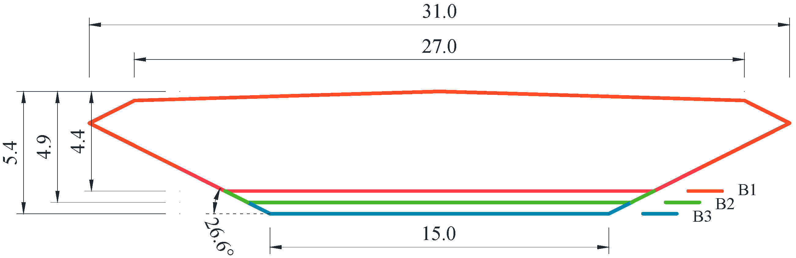
4.1. Numerical Model Verification

The aerodynamic forces of SBGs in a viscous flow are computed via numerical simulation. To ensure the validity of the numerical model, the simulation of B3 (i.e., the Great Belt East Bridge) was conducted first. A hybrid grid scheme of the structured grids and the unstructured grids with a total grid number of 291,202 was adopted, as presented in Figure 4. To simulate the motion of the SBG, the computational domain was divided into three regions, namely, the rigid mesh zone, dynamic mesh zone, and fixed mesh zone. The rigid mesh zone moved along with the SBG to ensure the quality of the mesh near the SBG. The normal spacing next to the SBG wall was 5 × 10⁻⁶ m. The height and width of the computational domain were 12 B and 18 B, respectively, in which B is the width of the SBG. The inlet boundary of the computational domain was set to the velocity inlet. The right boundary of the computational domain was set to the pressure outlet. The top and bottom boundaries were set as symmetry boundaries.
The ANSYS Fluent program was adopted to compute the aerodynamic forces of the SBG. Turbulence was modeled using the SST k-ω viscous scheme, and the PISO scheme was selected to solve the pressure–velocity coupling. The least-squares cell-based scheme was used to compute the gradient, while the second-order interpolation scheme was utilized for pressure approximation. Furthermore, the second-order upwind scheme was implemented for other spatial discretization terms. The dimensionless time step was set to 0.001 s to ensure accuracy.
For the sake of reliable numerical results, the numerical model must be validated. The forced single-degree-of-freedom vertical and pitching harmonic vibrations were carried out. The amplitude of the vibration was set at 0.02 B for vertical motion and 3° for pitching motion. The vibration frequency was 2.0 Hz for both the vertical and pitching vibrations. A comparison of the flutter derivatives is exhibited in Figure 5, for which the wind tunnel test was conducted by Reinhold et al. [38]. The flutter velocity is presented in Table 2. The results indicate that the flutter derivatives obtained from the numerical simulation are consistent with those from the wind tunnel test. The flutter critical wind velocity and the flutter frequency have errors of only 0.3% and 3.7%, respectively, compared to the experimental values. This suggests that the present numerical model demonstrates good accuracy in computing the aerodynamic forces of the SBG. Since B2 and B3 used the same mesh scheme and numerical settings as B1, it is reasonable to assume that their CFD-generated aerodynamic forces are also reliable.

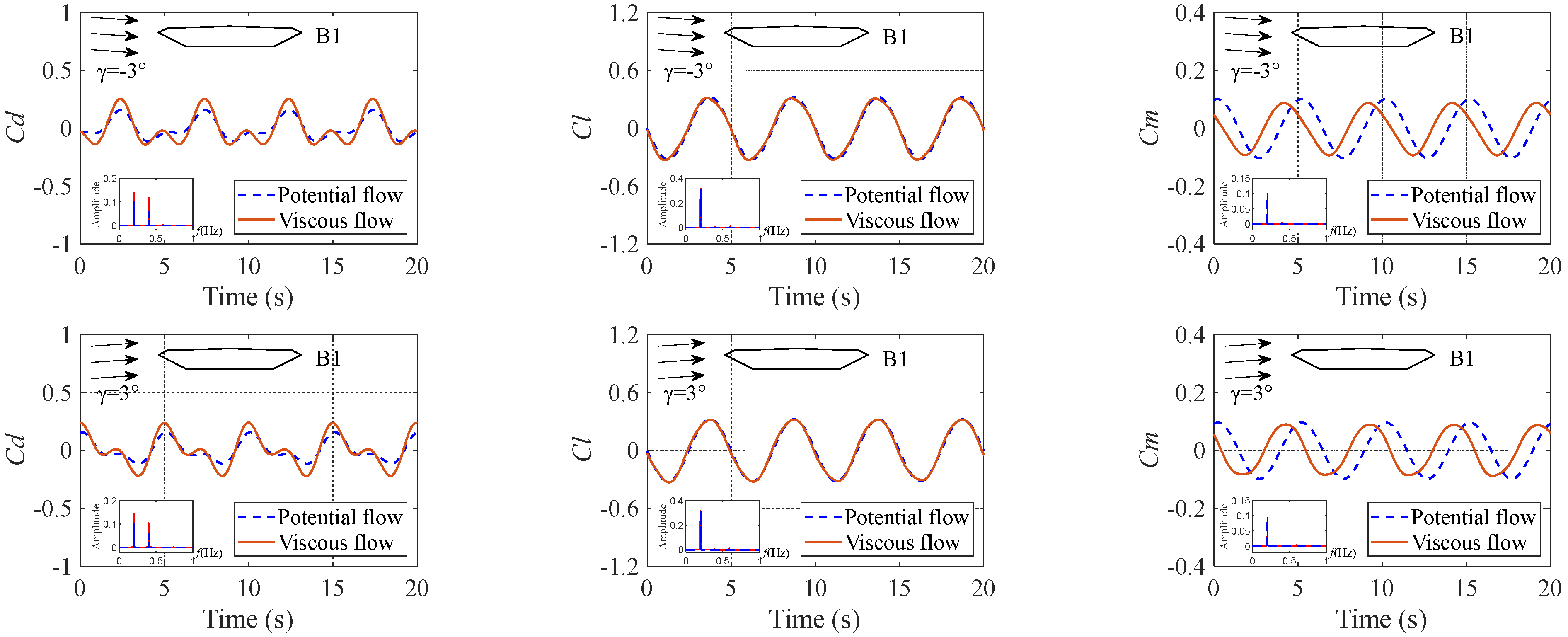
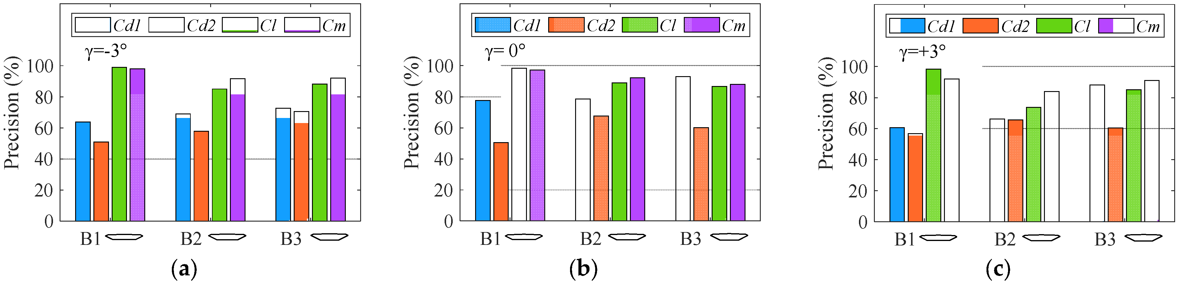
4.2. Aerodynamic Forces Comparative Analysis

The dimensionless aerodynamic coefficients Cd, Cl, and Cm are utilized to describe the aerodynamic forces on SBGs. The expressions of the aerodynamic coefficients are displayed in Equation (40), where V = 10.0 m/s is the wind velocity, and H means the height of the SBGs.
C d = F x / 0.5 ρ V 2 H ; C l = F y / 0.5 ρ V 2 B ; C m = M / 0.5 ρ V 2 B 2
Regarding the action of the wind load, assume that the SBGs are in the coupled vibration of u x = V + A x 2 π f cos 2 π f t , u y = A y 2 π f cos 2 π f t , and ω = A m 2 π f cos 2 π f t , where Ax = 0.01 B, A y = 0.02 B, A m = 3°, B = 31.0 m, f = 0.2 Hz, and t denotes time series. Figure 6 illustrates a comparison of the aerodynamic drag force, lift force, and pitching moment of three SBGs in both potential and viscous flows. The results reveal that the evolution law of aerodynamic force with time via the potential solution is close to the viscous flow. Since there is no flow separation in a potential flow, the drag force in a potential flow is smaller than the drag force in a viscous flow. However, the potential solution reproduces the second-order component of the drag force. The second-order effect was also observed before [16,22] and cannot be achieved by the Scanlan model [13], as expressed in Equation (41), where P i * (i = 1,3,5,6) represent the flutter derivatives related to the drag force. The second-order component is generated by ρ A ω u y and Re ρ ω 2 π i u ¯ k = 3 n 2 k c ¯ k c k + u c 1 c 3 in Equation (36), indicating that the second-order component is primarily caused by the multiplication of the vertical vibration velocity u y and the pitching vibration velocity ω.
For the lift force and pitching moment, the frequency is almost the same as the coupled vibration frequency f. There are also second-order components for the lift force and pitching moment in Equations (36) and (39), but they are too slight to be neglected. A similar phenomenon was reported before by Chen et al. [21]. The amplitudes of the lift force and the pitching moment of the potential flow solution are close to those of the viscous flow. However, in most cases, the aerodynamic force in a potential flow is smaller than the aerodynamic force in a viscous flow. Furthermore, the aerodynamic forces in a potential flow will lag behind those in a viscous flow. The phase lag of the pitching moment is the most salient observation, with a value of approximately 0.36π. However, it should be noted that this value exhibits slight variability across different SBG aspect ratios.
F d = 1 2 ρ U 2 2 B K P 1 * p ˙ U + K P 2 * B α ˙ U + K 2 P 3 α + K 2 P 4 p B + K P 5 h ˙ U + K 2 P 6 h B
The angle of attack effect can be determined by defining the motion of the SBG. Suppose that γ is the angle of attack; then, the lateral and vertical motion of the SBG can be expressed as u x = V cos γ + A x 2 π f cos 2 π f t and u y = V sin γ A y 2 π f cos 2 π f t . For the sake of brevity, only the aerodynamic coefficients of B1, with an angle of attack of ±3°, are exhibited in Figure 7. The results show that the drag force still has a second-order effect on the wind flow at the angle of attack of ±3°, and this phenomenon also appears in the potential flow solution. Additionally, the analytical solution for the potential flow can predict the amplitudes of the lift force and pitching moment in a viscous flow well. As a consequence, the proposed force model solution and the viscous CFD solution showcase remarkable similarities in the magnitude and frequency of the unsteady aerodynamic force. In view of these findings, the expressions in Equations (36) and (39) have the potential to serve as useful references in the development of an aerodynamic force model in a real flow.
The precisions of the amplitude of the aerodynamic forces by the potential theory are displayed in Figure 8, where Cd1 and Cd2 denote the first-order and second-order components of the drag force coefficients, respectively. The precision is defined in Equation (42), where Ap and Av are the amplitudes of the aerodynamic force coefficients in a potential flow and a viscous flow, respectively. It is observed that the precision of the first-order component of the drag force is higher compared to that of the second-order component. However, due to the neglect of viscosity, the drag force in the potential flow is lower than that obtained from the viscous flow. Generally, the precision level of the lift force and pitching moment are better than that of the drag force. Nevertheless, the precision levels of the lift force and pitching moment decrease with an increasing aspect ratio. The average precision levels of the lift force and pitching moment of B1 at the three angles of attack are 98.6% and 95.8%, respectively, indicating that the analytical solution can predict the lift force and pitching moment of an SBG with a small aspect ratio well. The potential flow solution is advantageous in terms of the computation time, which is less than one second when using Equations (36) and (39). Therefore, the analytical solution in a potential flow can be used for a rapid estimation of the aerodynamic forces on an SBG in coupled vibration.
p r c = 1 A p A v A v × 100 %

5. Conclusions

The aerodynamic force acting on the bridge structure has the potential to cause significant vibrations or even structural damage, thereby endangering the safety and reducing the sustainability of the bridge structure. In the present study, an analytical solution to the unsteady aerodynamic forces of the SBG was investigated based on the potential flow theory. The current study is distinguished from prior research by the comparatively intricate conformal mapping expression for SBGs, which resulted in discernable disparities in the aerodynamic force formulae. The complex potential and pressure functions were derived. The aerodynamic drag force, lift force, and pitching moment were expressed as functions of the motion state of the SBG and the conformal mapping coefficients. Subsequently, a numerical model was developed to simulate the wind field under a viscous flow. Finally, the analytical aerodynamic forces of three SBGs for different angles of attack were compared with the CFD viscous solution. The main conclusions are as follows:
(1)
The proposed analytical solution for the unsteady aerodynamic forces of an SBG with coupled vibration in a potential flow is a function of the SBG’s shape-related parameters and vibration response, providing a convenient and efficient method for calculating the unsteady aerodynamic forces of SBGs.
(2)
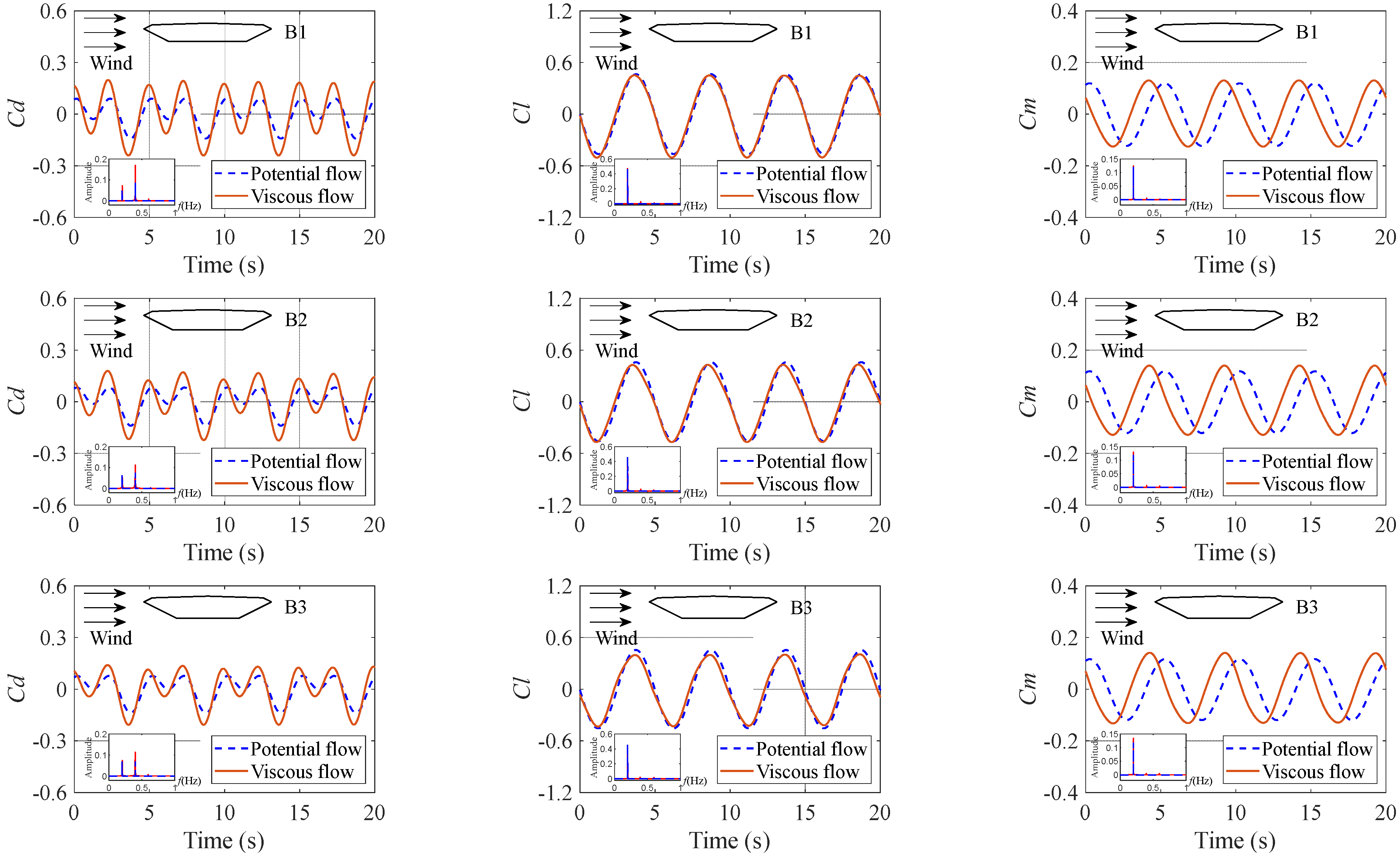
The analytical drag force successfully reproduced the second-order component, which mainly results from the multiplication of the vertical vibration and pitching vibration velocity terms and plays a significant role in drag force. On the other hand, the first-order frequency component dominates the lift force and pitching moment.
(3)
The proposed analytical solution for the drag force in a potential flow yields lower values than that in a viscous flow. Nonetheless, the analytical solution demonstrates high accuracy in predicting the amplitude of the lift force and pitching moment for an SBG at angles of attack of 0° and ±3°. The explicit formulation and satisfactory precision of the analytical solution enable its effective utilization for the rapid estimation of the aerodynamic forces acting on an SBG with coupled vibration.
(4)
It is imperative to underscore that the proposed analytical aerodynamic force model may not exhibit a sufficient degree of accuracy when applied to bluff bodies. It is noteworthy that the potential flow theory, which serves as the foundation for this model, is a linearized theory that may not fully capture the intricate nonlinear unsteady aerodynamic forces that manifest at high angles of attack and velocities or during large amplitude vibrations. In the future, there will be a greater focus on a more accurate aerodynamic force model for SBGs. To achieve this, further studies shall be conducted to investigate innovative correction methods.

Author Contributions

Conceptualization, L.W. and M.Z.; methodology, L.W.; validation, F.J. and Z.Z.; formal analysis, L.W.; investigation, L.W.; writing—original draft preparation, L.W.; writing—review and editing, M.Z. and Y.L.; visualization, F.J.; supervision, M.Z. and Y.L. All authors have read and agreed to the published version of the manuscript.

Funding

This research received no external funding.

Institutional Review Board Statement

Not applicable.

Informed Consent Statement

Not applicable.

Data Availability Statement

The data presented in this study are available upon request from the corresponding author.

Conflicts of Interest

The authors declare no conflict of interest.

References

  1. Liu, Y.; Wang, H.; Xu, Z.; Li, J.; Wu, T.; Mao, J. Modeling Multidimensional Multivariate Turbulent Wind Fields Using a Correlated Turbulence Wave Number–Frequency Spectral Representation Method. J. Eng. Mech. 2023, 149, 04023010. [Google Scholar] [CrossRef]
  2. Zhang, H.; Wang, H.; Xu, Z.; Zhang, Y.; Tao, T.; Mao, J. Monitoring-Based Analysis of Wind-Induced Vibrations of Ultra-Long Stay Cables during an Exceptional Wind Event. J. Wind. Eng. Ind. Aerodyn. 2022, 221, 104883. [Google Scholar] [CrossRef]
  3. Amer, T.S.; Bek, M.A.; Abouhmr, M.K. On the Vibrational Analysis for the Motion of a Harmonically Damped Rigid Body Pendulum. Nonlinear Dyn. 2018, 91, 2485–2502. [Google Scholar] [CrossRef]
  4. Bek, M.A.; Amer, T.S.; Sirwah, M.A.; Awrejcewicz, J.; Arab, A.A. The Vibrational Motion of a Spring Pendulum in a Fluid Flow. Results Phys. 2020, 19, 103465. [Google Scholar] [CrossRef]
  5. Amer, T.S.; Galal, A.A.; Elnaggar, S. The Vibrational Motion of a Dynamical System Using Homotopy Perturbation Technique. Appl. Math. 2020, 11, 1081–1099. [Google Scholar] [CrossRef]
  6. Zhang, J.; Zhang, M.; Jiang, X.; Wu, L.; Qin, J.; Li, Y. Pair-Copula-Based Trivariate Joint Probability Model of Wind Speed, Wind Direction and Angle of Attack. J. Wind Eng. Ind. Aerodyn. 2022, 225, 105010. [Google Scholar] [CrossRef]
  7. Li, Y.; Jiang, F.; Zhang, M.; Dai, Y.; Qin, J.; Zhang, J. Observations of Periodic Thermally-Developed Winds beside a Bridge Region in Mountain Terrain Based on Field Measurement. J. Wind Eng. Ind. Aerodyn. 2022, 225, 104996. [Google Scholar] [CrossRef]
  8. Diana, G.; Omarini, S. A Non-Linear Method to Compute the Buffeting Response of a Bridge Validation of the Model through Wind Tunnel Tests. J. Wind Eng. Ind. Aerodyn. 2020, 201, 104163. [Google Scholar] [CrossRef]
  9. Wu, L.; Woody Ju, J.; Zhang, J.; Zhang, M.; Li, Y. Vibration Phase Difference Analysis of Long-Span Suspension Bridge during Flutter. Eng. Struct. 2023, 276, 115351. [Google Scholar] [CrossRef]
  10. Cui, C.; Ma, R.; Hu, X.; He, W. Vibration Analysis for Pendent Pedestrian Path of a Long-Span Extradosed Bridge. Sustainability 2019, 11, 4664. [Google Scholar] [CrossRef]
  11. Amman, O.H.; von Kármán, T.; Woodruff, G.B. The Failure of the Tacoma Narrows Bridge; Federal Works Agency: Washington, DC, USA, 1941. [Google Scholar]
  12. Chen, A.; He, X.; Xiang, H. Identification of 18 Flutter Derivatives of Bridge Decks. J. Wind Eng. Ind. Aerodyn. 2002, 90, 2007–2022. [Google Scholar] [CrossRef]
  13. Scanlan, R.H.; Tomko, J.J. Airfoil and Bridge Deck Flutter Derivatives. J. Eng. Mech. 1971, 97, 1717–1737. [Google Scholar] [CrossRef]
  14. Ma, T.; Zhao, L.; Shen, X.; Ge, Y. Case Study of Three-Dimensional Aeroelastic Effect on Critical Flutter Wind Speed of Long-Span Bridges. J. Wind Eng. Ind. Aerodyn. 2021, 212, 104614. [Google Scholar] [CrossRef]
  15. Sauder, H.S.; Sarkar, P.P. A 3-DOF Forced Vibration System for Time-Domain Aeroelastic Parameter Identification. Wind Struct. 2017, 24, 481–500. [Google Scholar] [CrossRef]
  16. Xu, F.; Wu, T.; Ying, X.; Kareem, A. Higher-Order Self-Excited Drag Forces on Bridge Decks. J. Eng. Mech. 2016, 142, 06015007. [Google Scholar] [CrossRef]
  17. Guo, J.; Tang, H.; Li, Y.; Wu, L.; Wang, Z. Optimization for Vertical Stabilizers on Flutter Stability of Streamlined Box Girders with Mountainous Environment. Adv. Struct. Eng. 2020, 23, 205–218. [Google Scholar] [CrossRef]
  18. Kusano, I.; Cid Montoya, M.; Baldomir, A.; Nieto, F.; Jurado, J.Á.; Hernández, S. Reliability Based Design Optimization for Bridge Girder Shape and Plate Thicknesses of Long-Span Suspension Bridges Considering Aeroelastic Constraint. J. Wind Eng. Ind. Aerodyn. 2020, 202, 104176. [Google Scholar] [CrossRef]
  19. Zhou, Z.; Mao, W.; Ding, Q. Experimental and Numerical Studies on Flutter Stability of a Closed Box Girder Accounting for Ground Effects. J. Fluids Struct. 2019, 84, 1–17. [Google Scholar] [CrossRef]
  20. Zhang, M.; Xu, F.; Zhang, Z.; Ying, X. Energy Budget Analysis and Engineering Modeling of Post-Flutter Limit Cycle Oscillation of a Bridge Deck. J. Wind. Eng. Ind. Aerodyn. 2019, 188, 410–420. [Google Scholar] [CrossRef]
  21. Chen, Z.Q.; Yu, X.D.; Yang, G.; Spencer, B.F. Wind-Induced Self-Excited Loads on Bridges. J. Struct. Eng. 2005, 131, 1783–1793. [Google Scholar] [CrossRef]
  22. Siedziako, B.; Øiseth, O. Modeling of Self-Excited Forces during Multimode Flutter: An Experimental Study. Wind Struct. 2018, 27, 293–309. [Google Scholar] [CrossRef]
  23. Von Karman, T.; Sears, W.R. Airfoil Theory for Non-Uniform Motion. J. Aeronaut. Sci. 1938, 5, 379–390. [Google Scholar] [CrossRef]
  24. Theodorsen, T. General Theory of Aerodynamic Instability and the Mechanism of Flup; Twentieth Annual Report of the National Advisory Committee for Aeronautics; NACA: Washington, DC, USA, 1935; pp. 413–434. [Google Scholar]
  25. Edwards, J.W.; Ashley, H.; Breakwell, J.V. Unsteady Aerodynamic Modeling for Arbitrary Motions. AIAA J. 1979, 17, 365–374. [Google Scholar] [CrossRef]
  26. Sun, M.; Wang, W. Method for Calculating the Unsteady Flow of an Elliptical Circulation-Control Airfoil. J. Aircr. 1989, 26, 907–913. [Google Scholar] [CrossRef]
  27. Stangfeld, C.; Rumsey, C.L.; Mueller-Vahl, H.; Greenblatt, D.; Nayeri, C.; Paschereit, C.O. Unsteady Thick Airfoil Aerodynamics: Experiments, Computation, and Theory. In Proceedings of the 45th AIAA Fluid Dynamics Conference, Dallas, TX, USA, 22–26 June 2015. [Google Scholar]
  28. Catlett, M.R.; Anderson, J.M.; Badrya, C.; Baeder, J.D. Unsteady Response of Airfoils Due to Small-Scale Pitching Motion with Considerations for Foil Thickness and Wake Motion. J. Fluids Struct. 2020, 94, 102889. [Google Scholar] [CrossRef]
  29. Chiu, T.W. A Two-Dimensional Second-Order Vortex Panel Method for the Flow in a Cross-Wind over a Train and Other Two-Dimensional Bluff Bodies. J. Wind Eng. Ind. Aerodyn. 1991, 37, 43–64. [Google Scholar] [CrossRef]
  30. Chiu, T.W. Prediction of the Aerodynamic Loads on a Railway Train in a Cross-Wind at Large Yaw Angles Using an Integrated Two- and Three-Dimensional Source/Vortex Panel Method. J. Wind Eng. Ind. Aerodyn. 1995, 57, 19–39. [Google Scholar] [CrossRef]
  31. Valentine, D.T.; Madhi, F. Unsteady Potential Flow Theory and Numerical Analysis of Forces on Cylinders Induced by Nearby Oscillating Disturbances. In Proceedings of the American Society of Mechanical Engineers Digital Collection, Honolulu, HA, USA, 31 May–5 June 2009; pp. 631–639. [Google Scholar]
  32. Henrici, P. Cauchy Integrals on Closed Curves. In Applied and Computational Complex Analysis, Volume 3: Discrete Fourier Analysis, Cauchy Integrals, Construction of Conformal Maps, Univalent Functions; John Wiley & Sons: Hoboken, NJ, USA, 1993; pp. 113–119. [Google Scholar]
  33. Wu, L.; Zhou, Z.; Zhang, J.; Zhang, M. A Numerical Method for Conformal Mapping of Closed Box Girder Bridges and Its Application. Sustainability 2023, 15, 6291. [Google Scholar] [CrossRef]
  34. Wu, L.; Ju, J.W.; Zhang, M.; Li, Y.; Qi, J. Aerostatic Pressure of Streamlined Box Girder Based on Conformal Mapping Method and Its Application. Wind Struct. 2022, 35, 243–253. [Google Scholar] [CrossRef]
  35. Segletes, S.B.; Walters, W.P. A Note on the Application of the Extended Bernoulli Equation. Int. J. Impact Eng. 2002, 27, 561–576. [Google Scholar] [CrossRef]
  36. Katz, V.J. The History of Stokes’ Theorem. Math. Mag. 1979, 52, 146–156. [Google Scholar] [CrossRef]
  37. Larsen, A. Aerodynamic Aspects of the Final Design of the 1624 m Suspension Bridge across the Great Belt. J. Wind Eng. Ind. Aerodyn. 1993, 48, 261–285. [Google Scholar] [CrossRef]
  38. Reinhold, T.A.; Brinch, M.; Damsgaard, A. Wind Tunnel Tests for the Great Belt Link. In Proceedings of the Aerodynamics of Large Bridges: Proceeding of the First International Symposium on Aerodynamics of Large Bridges; Taylor & Francis: Copenhagen, Denmark, 1992; pp. 255–267. [Google Scholar]
  39. Honore Walther, J. Discrete Vortex Method for Two-Dimensional Flow Past Bodies of Arbitrary Shape Undergoing Prescribed Rotary and Translational Motion; Technical University of Denmark: Copenhagen, Denmark, 1994. [Google Scholar]
Figure 1. SBG in arbitrary coupled motion.
Sustainability 15 07312 g001
Figure 2. Moving and static coordinate system.
Sustainability 15 07312 g002
Figure 3. Sketch map of SBG shapes (unit: m).
Sustainability 15 07312 g003
Figure 4. Numerical simulation computational domain and mesh grid.
Sustainability 15 07312 g004
Figure 5. Comparison of flutter derivatives: (a) H i * (i = 1~4); (b) A i * (i = 1~4).
Sustainability 15 07312 g005
Figure 6. Comparison of aerodynamic forces.
Sustainability 15 07312 g006
Figure 7. Comparison of aerodynamic coefficients with angle of attack.
Sustainability 15 07312 g007
Figure 8. Precision of potential solution for different angles of attack: (a) γ = −3°; (b) γ = 0°; (c) γ = 3°.
Sustainability 15 07312 g008
Table 1. Conformal mapping coefficients.
SBG c 1 c 2 c 3 c 4 c 5 c 6 c 7 c 8 c 9 c 10
B18.79−0.57i6.450.45i−0.070.16i0.16−0.09i0.09−0.04i
B28.86−0.70i6.300.59i−0.010.16i0.18−0.12i0.06−0.02i
B38.93−0.82i6.160.72i0.070.13i0.19−0.14i0.030.01i
Table 2. Comparison of flutter critical velocity and frequency.
MethodWind Tunnel Test [38]Discrete Vortex Method [39]Present Simulation
Flutter critical velocity (m/s)37.635.337.5
Flutter frequency (Hz)0.1650.1650.159
Disclaimer/Publisher’s Note: The statements, opinions and data contained in all publications are solely those of the individual author(s) and contributor(s) and not of MDPI and/or the editor(s). MDPI and/or the editor(s) disclaim responsibility for any injury to people or property resulting from any ideas, methods, instructions or products referred to in the content.

