Article

Landscape Restoration Using Individual Tree Harvest Strategies

1
Forest Engineering, Resources, and Management Department, College of Forestry, Oregon State University, 3100 Jefferson Way, Corvallis, OR 97333, USA
2
Faculty of Silviculture and Forest Engineering, Transilvania University of Brasov, Sirul Beethoven 1, 500123 Brasov, Romania
*
Author to whom correspondence should be addressed.
Sustainability 2024, 16(12), 5124; https://doi.org/10.3390/su16125124
Submission received: 25 May 2024 / Revised: 10 June 2024 / Accepted: 11 June 2024 / Published: 16 June 2024
(This article belongs to the Special Issue Sustainable Forestry Management and Technologies)

Abstract

:
Western juniper (Juniperus occidentalis Hook.) is a native species west of the Rocky Mountains that has become noxious as its area increased ten times in the last 140 years. Restoration of the landscapes affected by the spread of juniper through harvesting poses several challenges related to the sparse spatial distribution (trees per hectare) of the resource. Therefore, the objective of the present study is to develop a harvest scheduling strategy that converts the western juniper from a noxious species to a timber resource. We propose a procedure that aggregates individual trees into elementary harvest units by considering the location of each tree. Using the coordinates of each harvest unit and its corresponding landing, we developed a spatially explicit algorithm that aims at the maximization of net revenue from juniper harvest. We applied the proposed landscape restoration approach to two areas of similar size and geomorphology. We implemented the restoration algorithm using two heuristics: simulated annealing and record-to-record travel. To account for the closeness to the mill, we considered two prices at the landing for the juniper: 45 USD/ton and 65 USD/ton. Our results suggest that restoration is possible at higher prices, but it is economically infeasible when prices are low. Simulated annealing outperformed record-to-record travel in both study areas and for both prices. Our approach and formulation to the restoration of landscapes invaded by western juniper could be applied to similar instances where complex stand structures preclude the use of traditional forest stand-level harvest scheduling and require a more granular approach.

1. Introduction

Western juniper (Juniperus occidentalis Hook.) is a native species west of the Rocky Mountains that has become noxious in Eastern Oregon [1]. The expansion of the western juniper is unprecedented [2], as its range has increased tenfold in the last 140 years [3]. The spreading out of western juniper changes the landscape not only by altering species composition but also by modifying the hydrological processes and wildlife habitat. Therefore, landscape restoration became important in many areas of Eastern Oregon, where western juniper canopy cover has increased more than fivefold since 1938 [4]. Currently, western juniper is removed using techniques typical to noxious species, such as manual felling and burning. In the past few decades, several mills have started processing western juniper, regardless of the complexity of stem shape [5]. With the establishment of a potential demand for western juniper, harvesting as a restoration technique becomes feasible, with the possibility that tree utilization will offset some of the restoration costs. Therefore, to make the restoration economically sound, a harvest system must be specified, a harvest plan developed, the needed infrastructure identified, and an estimate of the harvest costs and values estimated.
Applying traditional stand-level harvesting techniques to western juniper is challenging for several reasons, the first of which is its sparse and variable stand structure [6]. The seemingly erratic density across the landscape creates difficulties in the identification of relatively homogeneous stands. Furthermore, the complex terrain on which juniper thrives adds challenges to the development of feasible harvesting approaches [7]. Moreover, besides the sparse presence of junipers on the landscape and the difficult terrain, many junipers cannot be profitably harvested, as they lack the minimum merchantable wood volume needed to offset the costs associated with harvesting. Therefore, the consideration of individual trees allows for harvest without loss, and even with profit, by accepting solutions that exclude trees that are unprofitable to harvest. Remote sensing can reduce some of the costs not only by curtailing inventory expenses but also by helping increase the efficiency of planning the harvests [8,9,10,11,12]. The addition of information associated with remote sensing techniques was noticed for more than two decades [8] and improved harvest practices [10].
Several previous authors have considered harvesting at individual tree levels, but their studies were focused on stand management rather than landscape restoration [13,14,15,16,17,18]. The studies by Pukkala et al. [15], Pukkala and Miina [16], Vauhkonen and Pukkala [17], and Wing et al. [18] were focused on the selection of individual trees to be thinned using either a deterministic or a heuristic algorithm. The four investigations aimed at the optimization of revenue [15,16,17] or a criterion that combines volume, area, and edge [18] based on the size and location of the trees. Philippart et al. [14] used mixed integer programming to minimize total skidding distance in a semi-deciduous tropical forest in Cameroon where 3930 trees were located on 2562 ha, but the trees were referenced on a 20 m × 20 m grid. Dykstra’s shortest path algorithm was used to calculate skidding distances between candidate tree locations and landings, with the skidding distances used as a penalty. To reduce the problem size, the trees accessible to each landing were limited. The tree level problem addressed by Parsakhoo et al. [13] in the Hyrcanian forests of Iran also sought to minimize skid trail length to avoid environmental impacts using multi-objective criteria analysis and network programming but did not consider landing costs. A tree-level solution was proposed by Contreras and Chung [19] to reduce the crown fire potential in stands dominated by Douglas fir (Pseudotsuga menziesii (Mirb) Franco), ponderosa pine (Pinus ponderosa Dougl. ex Laws.), and western larch (Larix occidentalis Nutt). For fire management, the trees need to be spaced out so that the fire propagation is at least slowed down if not eliminated, whereas, for landscape restoration, the trees must be grouped so that economic feasibility is ensured. The methods developed in the studies presented above cannot be applied to landscape restoration as they are designed for small areas, specifically stand level. The usage of thousands of elementary management units in the previously mentioned studies led to computational challenges, which were addressed by simplification of the complex formulations. A common reduction in problem complexity is implemented by grouping trees, which can be done by pixels [14] or by economic criteria [19]. The main difference among the studies rests in the formulation of the planning problems, with some considering only economic attributes [15,16,17], while others consider additional facets of forest management, particularly the ecological aspect [19]. Landscape-scale problems add two levels of computational complexity that are not common to individual stands: first, an increased number of constraints that challenge the implementation of the problem and the rendering of a solution in a feasible amount of time, and second, a hierarchical structure that is difficult to formulate numerically without sacrificing problem simplicity. Therefore, the objective of this study was to develop a landscape-level restoration method that considers the individual tree as the elementary management unit. The tree level granularity allows the harvest schedule to adapt to the local conditions, expressed as tree density and geomorphology variations.

2. Materials and Methods

2.1. Study Areas

The landscape restoration strategy proposed in this study was tested on two areas of approximately 1600 ha in Wheeler County, Oregon (Figure 1): Pine Creek, with an elevation gradient of approximately 500 m, and Bridge Creek, with an elevation gradient of approximately 600 m (Table 1). The soils in the two basins are mainly Mollisols from the Palexerolls and Argixerolls Great Groups [20]. The climate is predominantly semiarid warm continental, according to Thornthwaite classification, with an average temperature of 11.3 °C (hottest month 30.5 °C and coldest month 5.5 °C), average rainfall of 390 mm, and average snowfall of 150 mm [16]. The detailed Köppen–Geiger classification places almost all of Wheeler County in two climates [21]: one warm-temperate [i.e., Cfa and Csa—Temperate (C) with hot summers (a) that can be without dry season (f) or dry summer (s)] and one arid [i.e., BSk—Arid (B) steppe (S) cold (k)]. The main tree species growing in these edaphic and climatic conditions is the western juniper, with spots of ponderosa pine (Pinus ponderosa Douglas ex C. Lawson).
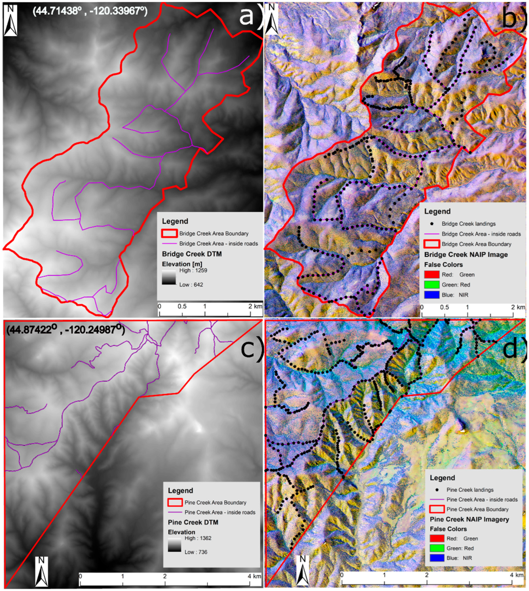
Complex terrain, understood as a multitude of small ridges (Figure 2a,c), dominates the study sites, which challenges the mobility of the equipment required for harvesting and processing western juniper [6]. To account for the unlikely movement of the harvested trees over significant ridges, we delineated the main sub-basins from the 10 m resolution digital terrain models (DTMs) provided by the US Geological Service [22]. The sub-basins were delineated with the D8 flow direction model based on the segment length threshold approach [23]. Having more variable geomorphology, the Pine Creek area was separated into 14 sub-basins, whereas the Bridge Creek area had 12 sub-basins.

2.2. Input Data

2.2.1. Individual Tree Location and Value

To identify each tree, we used the multispectral imagery supplied by the National Agriculture Imagery Program (NAIP) and two lidar-derived products provided by the Oregon Department of Geology and Mineral Industries (i.e., the digital surface model and the digital terrain model). The NAIP images have a resolution of 1 m and record four bands (i.e., red, green, blue, and near-infrared) with a radiometric resolution of 16 bits. Lidar collected from the Pine Creek area was used to generate a canopy height model, which, together with the multispectral imagery, constituted the input for locating individual trees [24]. We computed a canopy height model using a generative adversarial neural network [25] as implemented in pix2pix [26]. We located each tree by applying a Faster R-CNN (Regional Convolutional Neural Network) on the NAIP multispectral imagery and the canopy height model, as implemented in TensorFlow [27]. The combination of two algorithms, the generative adversarial neural network and the Faster R-CNN, identified the spatial coordinates of approximately 175,000 trees in the Pine Creek area and 160,000 trees in the Bridge Creek area [24]. The metrics used to assess the individual tree inventory were recall, precision, F1, omission error and commission error, similar to Strimbu and Strimbu [28] and Hao et al. [12]. The recall was 0.735, the precision 0.913, F1 0.824, the omission error 0.070, and the commission error 0.265. The 30 m pixel aggregated metrics were superior to the most recent study focused on juniper inventory in the area [29], which exhibited an 8.63% absolute error, whereas the convolutional neural network-based method produced only a 4.98% absolute error. Once the trees were positioned on the landscape, we estimated their height from the canopy height model created using the generative adversarial networks, which was, on average, 8.3 m for the Pine Creek area and 5.8 m for the Bridge Creek area (Table 2).
The combination of neural network algorithms was not accurate in species delineation (i.e., an accuracy of approximately 65%), which is likely the product of an unbalanced distribution of species (i.e., western juniper dominates the landscape) and a lack of nadir view throughout the image. Field survey and random NAIP image analysis revealed that more than 90% of the trees were western juniper, with only a small portion being other species, mostly ponderosa pine. Although other species are present in the study areas, for simplicity, we considered all trees to be western juniper. We chose to consolidate all the species to juniper to provide a conservative estimate for revenue, as ponderosa pine is more valuable than western juniper.
To identify the merchantable component of an individual juniper tree, we measured and harvested 26 trees, which were processed at the “In The Sticks” sawmill at Fossil, OR. The trees were selected randomly, the focus being on stems that provide revenue, expressed as merchantable timber. To estimate the value of each tree, we first measured the merchantable volume of each stem in cubic meters, then developed a linear model that relates the volume with the height of the juniper in meters (Equation (1)):
v o l u m e = 0.00708 × h e i g h t   [ m 3 ]
Local mills commonly buy western juniper by green weight. Therefore, from the landowner’s perspective, green weight is the measure used to estimate the potential value of harvested juniper. We converted the volume from Equation (1) to weight, assuming a density of 799.5 kg/m3. The density was obtained by converting the 499.6 kg/m3 density at 12% moisture content (dry basis), as estimated by Swan and Connolly [30], to a moisture content of 45% (wet basis), which approximates the freshly cut density of the junipers.
m a s s = 811 × V o l u m e   [ kg ]
Depending on the estimated weight of each juniper, we placed each tree into two categories: those that will be harvested and sent to a mill for processing and those that will be felled but left in the field. Many junipers are too small to be harvested profitably due to juniper’s dense crown [31]. However, these trees are still valuable from an ecological perspective, and this value is recognized by the US Department of Agriculture (USDA), which provides monetary incentives for juniper removal. Therefore, the final value of the harvested western junipers is the sum of the value of the merchantable timber plus the USDA incentives. Based on the costs of felling, processing, and skidding, the green weight threshold separating the western junipers reaching the mill from the one left on the ground was estimated to be 0.3 tons. The 0.3 tons tree weight ensures that all harvested trees would be profitable, given the costs and the revenue, as described in Dodson [6], at least to a landing. We computed the felling costs and the restoration value for all trees, but for trees above 0.3 tons, we also calculated the skidding and processing costs. To mimic the transportation costs, we considered two values, namely 65 USD/ton and 45 USD/ton. These values aimed to represent the distance to the processing facility, with closer mills having lower transportation costs and, therefore, higher values at the landing.

2.2.2. Landing Locations

Landing locations are truck-accessible points where logs can be loaded onto trucks for transport to the mill. Logs are skidded from their felling point to a landing. We identified the potential landing locations based on the improved and unimproved road network (Table 3). The improved roads in the two study areas are maintained gravel roads, whereas the unimproved roads are roads with limited or no maintenance (Figure 2). The unimproved tracks were digitized from the NAIP aerial imagery in ArcGIS 10.6.1 [32] (Environmental Systems Research Institute, 2008). In addition to the condition that the landings are along the existing roads (Figure 2), we considered four more criteria to represent reality accurately: (1) increased accessibility to western juniper, (2) the possibility of connecting unimproved and improved roads, (3) realistic positioning on the slope and landscape, and (4) the insurance of a distance of approximately 46 m (i.e., 150 feet) between landing locations. We selected the value of 46 m between landings to ensure continuous coverage of the entire area, as in the region, the minimum length of a landing is approximately 30 m (i.e., 100 feet), while the largest can reach 60 m (i.e., 200 ft).

2.3. Individual Tree Harvest Scheduling

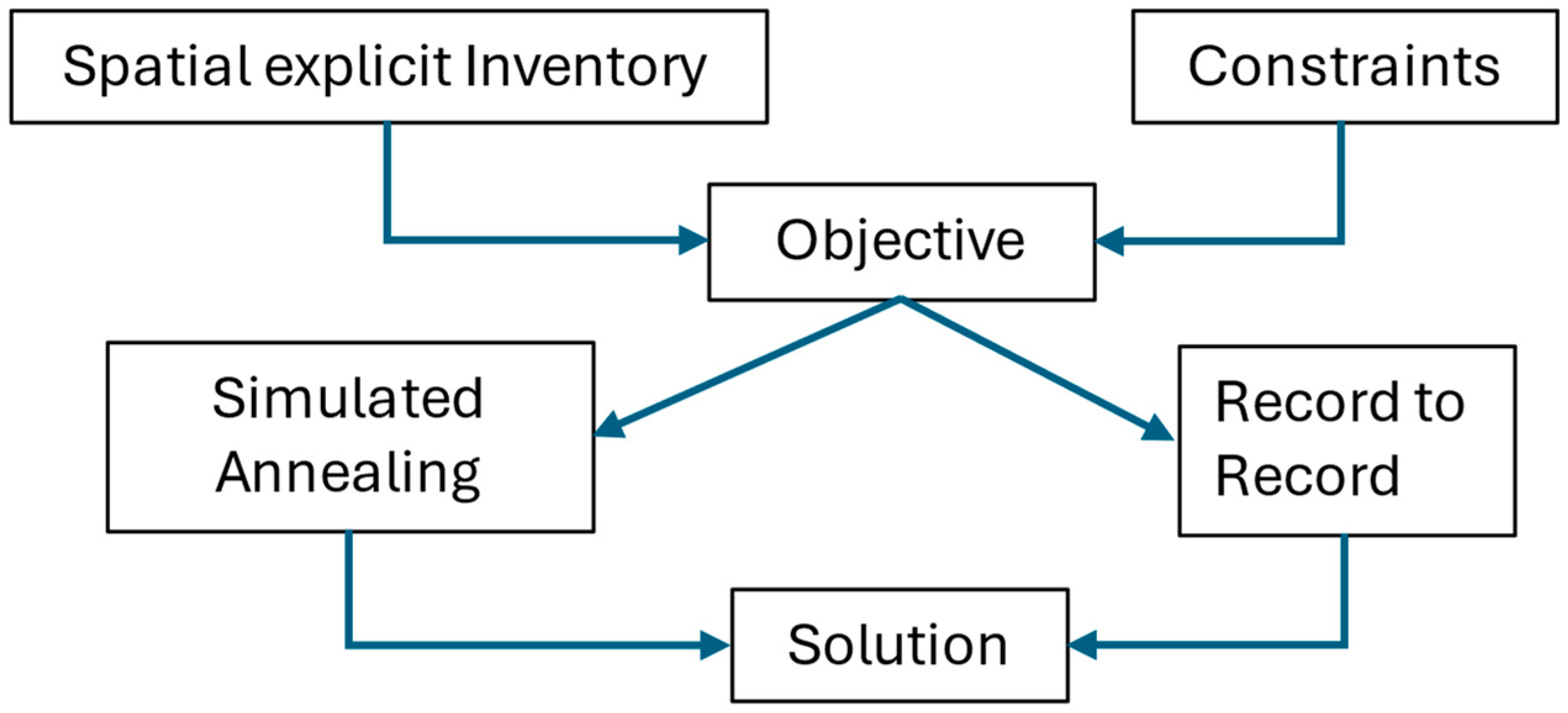
Spatially explicit forest planning problems using stands as elementary management units have polynomial complexity [33]. Therefore, planning problems that replace stands with individual trees have at least polynomial complexity. Considering that each individual tree and landing location is a distinct decision variable, the scale of this problem suggests the usage of heuristic methods rather than exact solutions, such as complete enumeration or mixed integer linear programming. To process the large number of possible solutions that select the trees to be harvested in a feasible computation time, we explore the use of two Monte Carlo-based optimization heuristics: simulated annealing [34,35], subsequently abbreviated to SA, and record-to-record travel [36], subsequently abbreviated to R2R (Figure 3). Both SA and R2R use a neighborhood search to find optimality, where each solution is a small modification of a previous solution. SA and R2R have been shown to lead to results close to an optimal solution for harvest scheduling [35,37]. Furthermore, SA and R2R are preferred over other heuristic optimization techniques, such as genetic algorithms or tabu search, because of their uncomplicated implementation [33,38].
The objective of our study was to maximize the net revenue, which is represented as the revenue from the tree scheduled to be harvested minus the costs associated with their harvesting, the cost of developing landing sites, and the hauling costs (Figure 3). The cost and revenue of each tree depend on two variables: the weight of the tree and the distance from the tree to the closest active landing. We modeled two scenarios for each area: one assuming the area is close to the mill (i.e., the value paid at the landing is 65 USD/green ton) and one that assumes the area is far from the mill (i.e., the value paid at the landing is 45 USD/green ton).

2.3.1. Harvest Costs

We modeled harvest costs based on the work by Dodson [6], which examined a series of harvest systems for western juniper in eastern Oregon. Felling and processing costs are both based on tree weight, while skidding costs are based on a combination of tree weight and distance to landing. Because many trees are felled for their restoration value rather than economic value, as assigned by the USDA, we also modeled the traveling costs associated with the harvesting equipment. A popular approach for estimating the distance from stump to landing is to estimate the centroid of the harvest unit and then compute the Euclidean distance between the centroid and landing. However, considering that in our case, the elementary management unit was the tree, which is represented by a point and not by a polygon, there was no meaningful centroid to be determined. To overcome the lack of area when individual trees are used as elementary management units, we observed that whenever the feller-buncher stops to harvest, all the trees within arm’s reach are cut and placed in one location, usually close to the previous stop. Therefore, the area reached by the feller-buncher can be considered as a harvest unit, the harvested trees being the elements on which the value is computed. Consequently, the centroid of the harvest unit is the location of the feller-buncher, which in actuality is the center of a circle with a radius defined by the arm of the feller-buncher. The expression of the hauling costs from stump to landing in these conditions is linearly related to the Euclidean distance between the coordinates of the feller-buncher when it stops to harvest and the coordinates of the landing. However, the study areas contain challenging terrain, which would be difficult to cross with some skidding equipment and whose cost would be erroneously modeled by the Euclidean distance. An unrealistic harvest situation is encountered when the trees from one basin are allocated to landings from another basin, which indicates a significant terrain change. To prohibit such situations, a penalty cost was applied when a change in basins between a landing and harvest unit occurred, which would encourage the algorithm to either select a different landing point or abandon that harvest unit. Considering the settings of our problem, we found that a penalty equal to that of skidding 3000 m was sufficient to prohibit the assignment of harvested trees to landings outside of their basin. Besides the variable hauling costs, there is a fixed cost associated with each landing for its construction. The current costs from Wheeler County suggest a cost of USD 500 per landing [39].

2.3.2. Spatial Implementation of the Harvests

Spatial considerations in scheduling harvests are often focused on ensuring that neighboring restrictions are not violated. Their achievement is commonly implemented with two approaches [40,41]: restricting harvests to adjacent units once an elementary management unit is cut, also known as a unit-restricted model, or restricting the size of the cut, also known as an area-restricted model. However, in our study, neither of the two constraints is applicable because the objective is landscape restoration by removing as many junipers as possible. Furthermore, spatial constraints impact the costs of harvest rather than the arrangements for harvests. To clear an area as large as possible, we started by defining the smallest area on which harvest could occur. We can naturally define such an area, which serves as an elementary planning unit, by referring to the capabilities of the equipment executing the felling. In this study, junipers were cut, processed, and piled with a feller-buncher, which can reach trees at most 7.6 m (i.e., 25 feet) from the operator [6]. Therefore, we define an elementary planning unit as a square with a side length of 15.24 m (i.e., 50 feet). The elementary planning units create a grid with a cell size of 232.26 m2 (i.e., 2500 ft2). We should point out that even though a grid is used for harvesting, scale is not a part of the analysis, as the cell size is defined by the forest operations and not analytically. Furthermore, no spatiality or generality was lost, as all the trees within a cell were harvested from one location, which we assumed to be in the center of the cell. Each grid cell is a harvest unit. After aggregating all trees within the grid cells, we reduced the problem complexity by not including the harvest units with costs that exceeded the value of the trees. If a harvest unit was not profitable, even assuming the closest possible landing point, then it was removed from the set of eligible harvests. In the eventuality that the minimum skidding load was not reached, the skidder would carry trees from more than one harvest unit to the landing.
The heuristic solution to scheduling problems usually starts by defining the solution space and the method by which the heuristic will move through it. In our problem, we had only two sets of decision variables: the set of harvest units, hu, which can be active or inactive, and the set of landings, l, which also can be active or inactive. An active landing or harvest unit means that logs are stored or harvest occurs, whereas an inactive unit is the opposite (i.e., no logs and no harvest). Given the decision variables, the movement through the solution space occurs in two directions: (1) a harvest unit can switch between the active and inactive set, and (2) a landing can move between the active and inactive status. In our formulation, we enforced at least one active landing, which ensures that when only one element is in the active landing set, it cannot be moved into the inactive set. The set of active harvest units and active landing make up a solution. The formulation of the landing selection is similar to that of Anderson and Nelson [42] and Philippart et al. [14] in the sense that each location was represented by a binary variable. However, since the restoration problem is spatially explicit, any change in the status of a landing (e.g., from active to inactive) triggers the re-computation and, consequently, reallocation of each harvest unit to the new set of active landings. The repeated estimation of all harvest unit–active landing pairs, even though it has a polynomial complexity, increases the time to obtain a solution from minutes to hours (i.e., on a Dell Precision 7910 workstation with a Xeon E5-263 v3 CPU and 32 GB RAM, it took approximately 8 h).
The heuristic algorithms selected to solve the scheduling problem are stochastic, and therefore, the moves through the solution space are executed according to a preset probability [43]. A possible move can occur if a random uniform variable in the set (0, 1] is smaller than the probability defining the heuristic, which depending on the algorithm have multiple forms [44].

2.3.3. Formulation of the Harvest Problem

The objective function is to maximize net revenue from all active harvest units:
m a x ( 1 a h u ( F V i + H V i ) ( E Q M C i + F C i + P C i + S K C i ) 1 a l L C j )
subject to
  • Harvest weight = sum of weights of trees with weight > 0.3 tons;
  • Non-harvest weight = sum of weights of trees with weight ≤ 0.3 tons;
  • Distance to closest active landing = Euclidean distance from the centroid of harvest unit to landing;
  • The monetary values of the attributes used to compute the net revenue of each harvest unit are presented in Table 4.
where
ahu is the number of active harvest units;
al is the number of active landings;
subsidy value of harvest unit i (FVi) = number of trees in harvest unit i × felling value subsidy;
harvested value of harvest unit i (HVi) = weight of merchantable volume in harvest unit i × harvest value coefficient;
feller-buncher moving cost of harvest unit i (EQMCi) = distance to closest active landing × equipment moving coefficient to harvest unit i;
felling cost in harvest unit i (FCi) = non-harvest weight × non-harvest felling coefficient + harvest weight × harvest felling coefficient;
processing cost in harvest unit i (PCi) = harvest tree weight × processing coefficient;
skidding cost from harvest unit i (SKCi) = harvest tree weight of unit i× (distance to closest active landing × skidding distance coefficient + skidding coefficient);
cost of building landing j (LCj) = constant.
Table 4. Juniper harvest costs and values used to estimate the net revenue at landing.
AttributeValueUnitsShort Description and Source
Felling subsidy2.0USD/treeEstimated USDA remediation value [45]
Value of merchantable tree65USD/tonEstimated value of a tree [46]
Feller-buncher and processor moving cost0.03USD/mEstimated cost of moving the feller-buncher and processor within the harvested area (authors)
Non-merchantable tree felling cost12USD/green tonCost of felling a non-merchantable tree [6]
Merchantable tree felling cost10USD/green ton Cost of felling a merchantable tree [6]
Merchantable tree processing cost15USD/green tonCost of processing a merchantable tree [6]
Skidding distance coefficient0.18USD/m/green tonDistance-related cost of moving merchantable juniper to the landing [6]
Skidding coefficient20USD/green tonNon-distance related skidding activities [6]
Landing cost500USD/landingCost of preparing a landing area [39]

2.3.4. Simulated Annealing

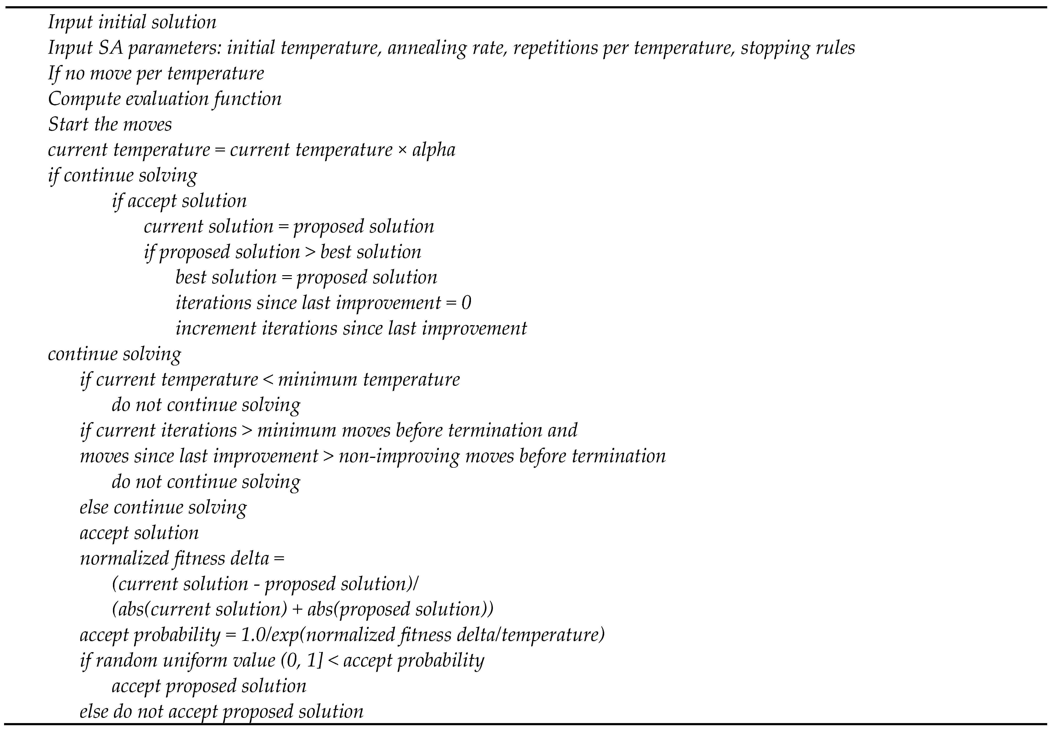
SA is a heuristic technique based on the idea that negative deviation from the current solution should decrease as the number of iterations increases [34,35,47]. SA has been widely applied in combinatorial optimization, cited second only to genetic algorithms, and well ahead of other combinatorial heuristics (Google Search 23 December 2018). SA is analogous to the annealing process through cooling in the sense that at higher temperatures, molecules have more energy. Therefore, they are able to move substantially, while later, when the temperature decreases, the energy is reduced, and the molecules move less. SA is mathematically represented through an exponential function and a ‘temperature’ variable, which allows for a large negative deviation for high temperatures and a small negative deviation when the temperature is small. SA is driven by at least four parameters [43,48,49]: annealing rate, initial temperature, number of moves at each temperature, and the stopping rule. The identification of proper parameters has a significant role in SA performance [50]. We chose the parameters using trial and error; the chosen parameters are the following:
Annealing rate:0.99
Initial temperature:0.25
Number of moves/temperature:200
Stopping rule: freezing temperature of 0.00001 or no improvement for 10,000 moves (~5% of the possible moves), whichever occurred first. If SA reached the freezing temperature, 201,000 moves were executed.
We found that normalizing the deviation between neighboring solutions by the current solution value provided consistent results. This normalization, which bounded the solution fitness deltas between −1 and 1, is the reason for the low initial temperature. The full description of the SA implementation, including the normalization, is shown in the pseudocode form Appendix A (Figure A1).

2.3.5. Record-to-Record Travel

R2R is a stochastic optimization heuristic that allows for a change in the current solution if it is not worse than the best-observed solution by a specified percentage [36]. R2R is a hill-climbing heuristic that is selected as a possible solution, which does not improve the current solution within a preset value called deviation. The major advantage of R2R over other heuristic methods is the reduced number of parameters to tune: the allowed deviation and the ending of the algorithm. To find the values suitable for our problem, we used a trial-and-error approach, which is common in the application of heuristic techniques [50]. We found that a deviation of 10% from the best-observed solution and an exploration of 200,000 moves supplies acceptable solutions. We also implemented an additional stopping rule based on the non-improvement of the solution. If the best solution did not improve after 10,000 moves or 5% of the total possible moves, similar to Zomaya and Kazman [51], we terminated the heuristic under the assumption that the optimum value for this run had been reached. To avoid premature termination, we enforced the 10,000 moves stopping rule after 150,000 moves. At the termination of the algorithm, the best solution was chosen as the output of the heuristic. A pseudocode description of the R2R implementation is shown in Appendix B (Figure A2).
Being heuristic, SA and R2R can supply close or far from optimal solutions, although well-chosen parameters and sufficient moves have been shown to produce high-quality solutions in other applications. We ran SA and R2R on the Amazon Web Service Cloud. SA terminated in about 4 h and RTR in about 2 h. For the 65 USD/ton price, we ran 29 solutions from different random number starts, and for the 45 USD/ton price, we terminated at 10 solutions because their solution values were closely grouped.

3. Results

One method for evaluating the quality of a heuristic solution is to see how close it is to a known upper or lower bound on the solution. For maximization problems, the interest is the upper bound. For complex problems solved with mixed integer linear programming, the upper bound is represented by the solution of a simplification of the original problem through the relaxation of some of the constraints. In this problem, the upper bound can be computed analytically under the assumptions of a given price per ton and ignoring the landing construction costs. Under these assumptions, each tree will travel to the closest possible landing, and trees with negative values will be dropped from the solution. It is not feasible in the sense that the landing costs are not considered. Subtracting the landing costs from the chosen landings in the upper bound solution provides a feasible lower bound. Another approach for measuring the quality of this heuristic is to compare the solution to the necessary conditions for optimizing skidding distance under a uniform distribution of harvest volume. For two-way skidding to evenly spaced discrete landings, the necessary conditions for existing roads are that the average skidding cost (USD/ton) is equal to twice the landing cost (USD/ton) [52]. We would expect the optimal solution to be near, although not equal to, these conditions given a non-uniform distribution of juniper trees.

3.1. Price at 65 USD/ton at the Landing

For USD 65 per ton, the upper bound on the net revenue was USD 559,281 for the Pine Creek area and USD 289,752 for the Bridge Creek area. The lower bound, obtained by subtracting the costs of the landings from the upper bound, was USD 359,781 for the Pine Creek area and USD 117,752 for the Bridge Creek area. The results of the 29 runs show the existence of a large number of solutions below the lower bound for each area for both algorithms (Table 5).
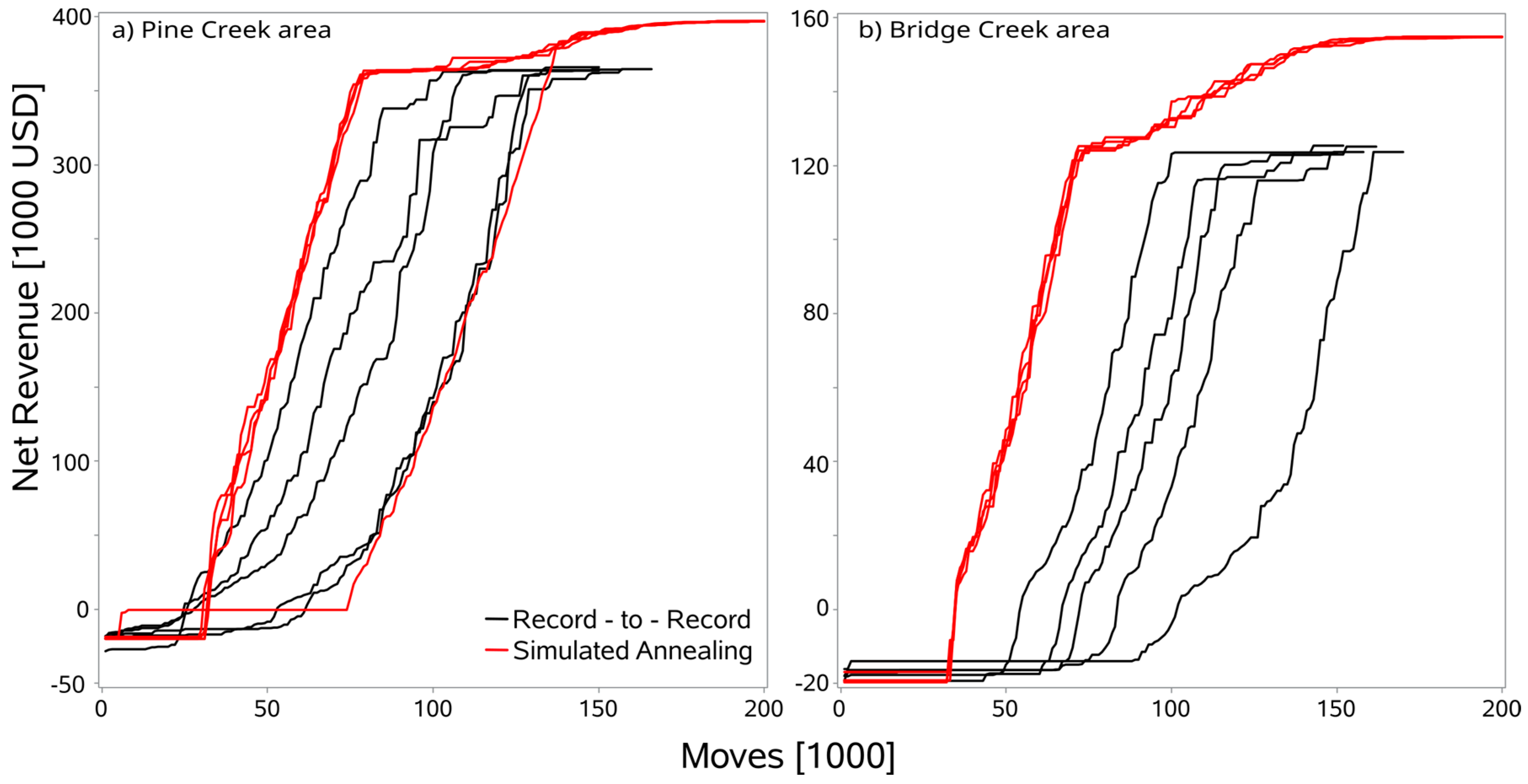
The best solutions revealed consistent results, with the R2R terminating because the solution did not improve for more than 10,000 moves, whereas SA ended when the freezing temperature was reached (Figure 4). Nevertheless, for both areas, the SA solutions did not improve more than 1% for the last 40,000 moves, which suggests, for the parameters chosen, that increasing the number of moves will not significantly improve the objective function.
At 65 USD/ton, SA supplied results that were more than 10% better than R2R. The weak performance of R2R likely reflects the algorithm’s disposition to investigate areas of the solution space with low juniper values (Figure 5), which led to a large number of solutions far from optimal. For both algorithms and study areas, the best solutions averaged at least one full truckload (20 tons) at each active landing (Table 6). We also see that the best R2R solution had significantly more landings than the solutions chosen by SA, which contributed to lower volume/landing and skidding distance/landing (Table 6).
As a check on the SA solution for Bridge Creek using the necessary conditions from Peters [52], the average landing cost (USD/ton) was 5.56 USD/ton (USD 500/90 tons = 5.56 USD/ton) (Table 6). The variable cost of skidding was 12.8 USD/ton (71.1 m × 0.18 USD/ton-m = 12.8 USD/ton). Thus, two times the landing cost, 11.12 USD/ton, is approximately equal to the skidding cost of 12.8 USD/ton, with a ratio of 0.87. The R2R solution had a more unbalanced landing-to-skidding cost, with an average landing cost of 7.69 USD/ton and an average skidding cost of 11.73 USD/ton, and the ratio was 1.31.

3.2. Price at 45 USD/ton at the Landing

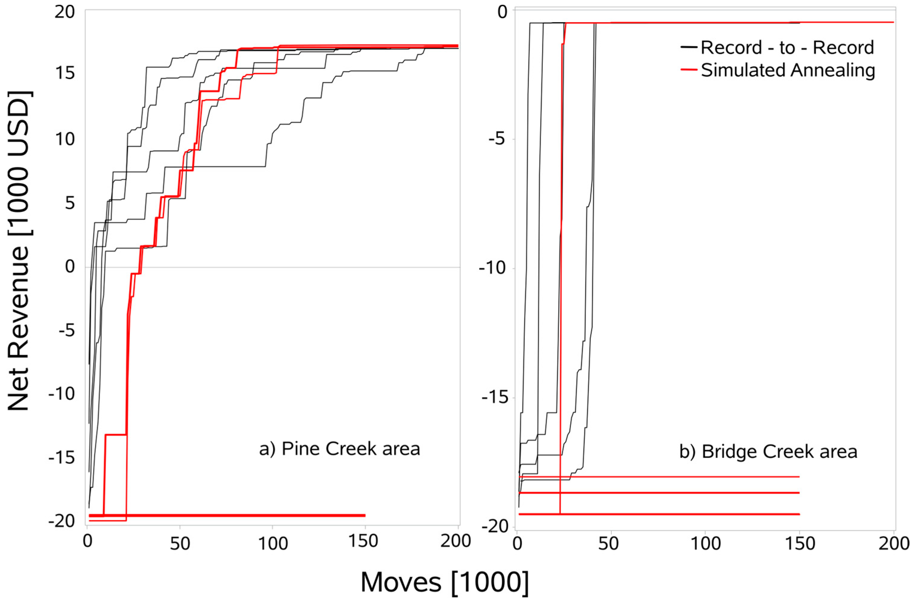
The upper and lower bounds defining the solution for 45 USD/ton are USD 37,049 and USD −162,451 for the Pine Creek area and USD 9861 and USD −162,139 for the Bridge Creek area, which not only are small in comparison to the 65 USD/ton but are also nearly unfeasible from an economic perspective. The summary statistics for the 45 USD/ton runs (Table 7) resulted in a very different picture than the 65 USD/ton. First, all solutions were above the lower bound. Second, the solutions were very different for the two areas, with Pine Creek having a positive net revenue and Bridge Creek having a negative net revenue. The negative net revenue is the result of the requirement that at least one landing is active. At a 45 USD/ton landing value, SA was about the same as R2R (Table 7).

4. Discussion

Landscape restoration poses logistic and financial challenges, which can sometimes be achieved simultaneously. In the case of western juniper in Eastern Oregon, the main challenge is economic, as the terrain is flatter than in Western Oregon. To ensure that restoration is economically feasible, we have implemented a unique approach that uses individual trees as the elementary management unit. Because we assumed that the trees are harvested with a boom-mounted harvesting and processing head, we grouped them according to the arms’ reach of the feller-buncher that executes the cuttings. The complexity induced by the usage of individual trees as elementary management units recommends the usage of heuristic algorithms to maximize the net revenue, which is the objective function. Among the many heuristic algorithms available, we selected simulated annealing and record-to-record travel based on the large number of studies reporting their superior performances [33,48,50,53,54,55,56,57]. Our formulation of the restoration problem showed that SA performed 10 to 20% better than R2R travel (Table 5) when the price was USD 65 per green ton but less than 5% when the price was USD 45 per green ton (Table 7). We believe that the weak performance of R2R with respect to SA is that R2R runs ended with the non-improvement stopping rule rather than reaching the preset maximum iterations. This indicates that the R2R runs were more likely to be trapped in a sub-optimal region of the solution space, which has more active landings in the final landing set. This outcome is likely due to the complexity and number of steps required for the heuristic to remove a landing in our algorithm formulation. Later in the run, when there is a higher number of harvest units in the active set, eliminating a landing increases the skidding costs, as all harvest units assigned to the eliminated landing are reassigned to the next closest landing. Therefore, removing a landing can lead to a momentary reduction of net revenue, which can subsequently yield a better overall solution. To mitigate the temporary net revenue loss, we allowed the harvest units to have zero net revenue for a small number of moves or until a closer landing was activated. Nevertheless, even with enhancements, the formulation of the scheduling problem indicates that R2R was not able to explore the solution space as effectively as SA.
Irrespective of the area and algorithm, the solutions are separated into two classes: one that contains solutions close to the global optima and one that encompasses solutions trapped in a local minimum. The solutions trapped in a local minimum either contained only one active landing or were below but close to the lower limit. Only one active landing was a common case for a trapped solution due to the fixed cost of establishing a new landing (USD 500), which in these cases was larger than the allowed R2R deviation. In the case of solutions slightly below the lower bound, we observed that the solution was trapped in a local minimum for the first 100,000 iterations, followed by a plateau near the 150,000 iterations. The runs ended around iteration 160,000 because of the stopping rule that terminates a run after 10,000 iterations without improvement. If this rule had not been in place, it is possible that more solutions would have exceeded the lower bound.
From the experiments with the reduced value per ton of western juniper, we see that the value per ton has a significant effect on the final solution, which consequently is reflected in the ability to restore the landscape or not. While USD 65 per ton supports a strong restoration process, a drop by one-third to USD 45 per ton suggests the inability to restore the landscape without additional support. The large drop in the solution value produced by the USD 20 per ton reduction in juniper price suggests that a relatively small change in juniper price may have a dramatic effect on the overall profitability of harvesting.
The method developed in the present study can be applied in other settings where the harvest units are individual trees, such as tropical forests. The requirement for individual trees as elementary planning units is imposed either by natural settings, the case of sparse forest (i.e., western juniper) or by high-value individuals, like redwoods (Sequoia sempervirens), Douglas firs (Pseudotsuga menziesii), or western red cedars (Thuja plicata). While we used Euclidean distance to develop skidding costs, more detailed travel models could be implemented through preprocessing of route costs and clustering techniques to keep all route information available in random-access memory.

5. Conclusions

Restoration of the landscapes affected by the spread of western juniper through harvesting poses a number of challenges related to the sparse spatial spread of the juniper trees. Therefore, the development of a harvest scheduling strategy is an important step towards viewing western juniper as a merchantable resource rather than a noxious species. Consequently, we propose a procedure that aggregates individual trees into elementary harvest units by considering the location of each tree. Using the location of each harvest unit and its corresponding landing, we formulated a spatially explicit algorithm that aims at the maximization of the net revenue while considering felling, processing, and skidding costs. We applied the proposed landscape remediation approach to two areas of similar size and terrain but with different tree distributions. Given the complexity of the individual tree-level scheduling, we used two heuristics, simulated annealing and record-to-record travel, to implement the restoration algorithm. Our results suggest that restoration is possible when the price is USD 65 per ton. The two scenarios for juniper value (i.e., negligible transportation costs vs. significant transportation costs) imply that the economically feasible solutions are highly dependent on the hauling distance between the landing and the mill; the farther the landing is from the mill, the closer to the landing the juniper tree must be to be viable.
Ultimately, we found that the complexity of the solution space led to simulated annealing, outperforming record-to-record travel in both of our study areas. Our approach and formulation to the restoration of landscapes invaded by western juniper could be applied to similar problem sets where complex stand structures preclude the use of traditional stand-level harvest scheduling and instead require a more granular system. Similarly, the method could be used for other harvesting systems, such as manual chainsaw felling and the use of rubber-tired choker skidders, farm tractors or other vehicles dragging logs or pulling small trailers.
While we examined scenarios based on the price paid at the landing, the method could be extended to the price paid at the mill. The small log volumes per landing in these examples suggest that a self-loading truck might be preferable to a separate loader. A study of transport distance, truckload capacity with and without a self-loader, and landing mobilization costs for separate loaders could focus future research.

Author Contributions

Conceptualization, J.S. and B.M.S.; methodology, R.S.; software, R.S.; validation B.M.S. and J.S.; formal analysis, R.S.; resources, J.S.; writing—original draft preparation, B.M.S. and R.S.; writing—review and editing, B.M.S. and J.S.; visualization, R.S. and B.M.S.; supervision, B.M.S. and J.S.; project administration, J.S.; funding acquisition, J.S. All authors have read and agreed to the published version of the manuscript.

Funding

This work was supported by the SUN grant of the US Department of Agriculture number 2014-38502-22598 and by the College of Forestry, Oregon State University.

Institutional Review Board Statement

Not applicable.

Informed Consent Statement

Not applicable.

Data Availability Statement

All the imagery used in this study is freely available online on the USDA NAIP website. The URL is https://naip-usdaonline.hub.arcgis.com/ (accessed on 8 June 2024). The elevation data are freely available on the Oregon Department of Geology and Mineral Industries, which has the URL https://www.oregon.gov/dogami/lidar/Pages/index.aspx (accessed on 8 June 2024).

Conflicts of Interest

The authors declare no conflicts of interest.

Appendix A

Figure A1. Pseudocode for simulated annealing implementation.
Sustainability 16 05124 g0a1

Appendix B

Figure A2. Pseudocode for record-to-record implementation.
Sustainability 16 05124 g0a2

References

  1. Durfee, N.; Ochoa, C.G.; Mata-Gonzalez, R. The Use of Low-Altitude UAV Imagery to Assess Western Juniper Density and Canopy Cover in Treated and Untreated Stands. Forests 2019, 10, 296. [Google Scholar] [CrossRef]
  2. Knapp, P.A.; Soulé, P.T. Recent Juniperus occidentalis (Western Juniper) Expansion on a Protected Site in Central Oregon. Glob. Chang. Biol. 1998, 4, 347–357. [Google Scholar] [CrossRef]
  3. Miller, R.F.; Bates, J.D.; Svejcar, T.J.; Pierson, F.B.; Eddleman, L.E. Biology, Ecology, and Management of Western Juniper (Juniperus occidentalis); Oregon State University: Corvallis, OR, USA, 2005; p. 82. [Google Scholar]
  4. Miller, R.F.; Rose, J.A. Historic Expansion of Juniperus occidentalis (Western Juniper) in Southeastern Oregon. Great Basin Nat. 1995, 55, 37–45. [Google Scholar]
  5. Swan, L. Western Juniper Furniture Market Research and Design Project; US Forest Service: Klamath Falls, OR, USA, 1998; p. 17.
  6. Dodson, E. A Comparison of Harvesting Systems for Western Juniper. Int. J. For. Eng. 2010, 21, 40–47. [Google Scholar] [CrossRef]
  7. Dodson, E.M.; Deboodt, T.; Hudspeth, G. Production, Cost, and Soil Compaction Estimates for Two Western Juniper Extraction Systems. West. J. Appl. For. 2006, 21, 185–194. [Google Scholar] [CrossRef]
  8. Hyyppa, J.; Kelle, O.; Lehikoinen, M.; Inkinen, M. A Segmentation-Based Method to Retrieve Stem Volume Estimates from 3-D Tree Height Models Produced by Laser Scanners. IEEE Trans. Geosci. Remote Sens. 2001, 39, 969–975. [Google Scholar] [CrossRef]
  9. Gatziolis, D.; Andersen, H.-E. A Guide to LiDAR Data Acquisition and Processing for the Forests of the Pacific Northwest; USDA—Forest Service, Pacific Northwest Reserach Station: Portland, OR, USA, 2008; p. 32.
  10. Liu, S.; Cieszewski, C.J. Impacts of Management Intensity and Harvesting Practices on Long-Term Forest Resource Sustainability in Georgia. Math. Comput. For. Nat.-Resour. Sci. 2009, 1, 52–66. [Google Scholar]
  11. Wang, H.; Yang, T.-R.; Waldy, J.; Jr, J.A.K. Estimating Individual Tree Heights and Dbhs from Vertically Displaced Spherical Image Pairs. Math. Comput. For. Nat.-Resour. Sci. 2021, 13, 1–14. [Google Scholar]
  12. Hao, Z.; Lin, L.; Post, C.J.; Mikhailova, E.A.; Li, M.; Chen, Y.; Yu, K.; Liu, J. Automated Tree-Crown and Height Detection in a Young Forest Plantation Using Mask Region-Based Convolutional Neural Network (Mask R-CNN). ISPRS J. Photogramm. Remote Sens. 2021, 178, 112–123. [Google Scholar] [CrossRef]
  13. Parsakhoo, A.; Mostafa, M.; Shataee, S.; Lotfalian, M. Decision Support System to Find a Skid Trail Network for Extracting Marked Trees. J. For. Sci. 2017, 63, 62–69. [Google Scholar] [CrossRef]
  14. Philippart, J.; Sun, M.; Doucet, J.-L.; Lejeune, P. Mathematical Formulation and Exact Solution for Landing Location Problem in Tropical Forest Selective Logging, a Case Study in Southeast Cameroon. J. For. Econ. 2012, 18, 113–122. [Google Scholar] [CrossRef]
  15. Pukkala, T.; Lähde, E.; Laiho, O. Which Trees Should Be Removed in Thinning Treatments? For. Ecosyst. 2015, 2, 32. [Google Scholar] [CrossRef]
  16. Pukkala, T.; Miina, J. Tree-Selection Algorithms for Optimizing Thinning Using a Distance-Dependent Growth Model. Can. J. For. Res. 1998, 28, 693–702. [Google Scholar] [CrossRef]
  17. Vauhkonen, J.; Pukkala, T. Selecting the Trees to Be Harvested Based on the Relative Value Growth of the Remaining Trees. Eur. J. For. Res. 2016, 135, 581–592. [Google Scholar] [CrossRef]
  18. Wing, B.M.; Boston, K.; Ritchie, M.W. A Technique for Implementing Group Selection Treatments with Multiple Objectives Using an Airborne Lidar-Derived Stem Map in a Heuristic Environment. For. Sci. 2019, 65, 211–222. [Google Scholar] [CrossRef]
  19. Contreras, M.A.; Chung, W. Developing a Computerized Approach for Optimizing Individual Tree Removal to Efficiently Reduce Crown Fire Potential. For. Ecol. Manag. 2013, 289, 219–233. [Google Scholar] [CrossRef]
  20. Soil Survey Staff. Soil Taxonomy, a Basic System of Soil Classification for Making and Interpreting Soil Surveys; USDA—NRCS: Alexandria, LA, USA, 1999; p. 886.
  21. Millison, A. Climate Classification Systems. In Permaculture Design Tools for Climate Resilience; Oregon State University: Corvallis, OR, USA, 2018; pp. 28–38. [Google Scholar]
  22. Archuleta, C.-A.M.; Constance, E.W.; Arundel, S.T.; Lowe, A.J.; Mantey, K.S.; Phillips, L.A. The National Map Seamless Digital Elevation Model Specifications; US Geological Service: Reston, VA, USA, 2017; p. 50.
  23. O’Callaghan, J.F.; Mark, D.M. The Extraction of Drainage Networks from Digital Elevation Data. Comput. Vis. Graph. Image Process. 1984, 28, 323–344. [Google Scholar] [CrossRef]
  24. Schriver, R. Landscape Inventory and Harvest Strategies for Individual Western Juniper in Eastern Oregon. Master’s Thesis, Oregon State University, Corvallis, OR, USA, 2018. [Google Scholar]
  25. Goodfellow, I.J.; Pouget-Abadie, J.; Mirza, M.; Xu, B.; Warde-Farley, D.; Ozair, S.; Courville, A.; Bengio, Y. Generative Adversarial Networks. arXiv 2014, arXiv:1406.2661. [Google Scholar] [CrossRef]
  26. Isola, P.; Zhu, J.-Y.; Zhou, T.; Efros, A.A. Image-to-Image Translation with Conditional Adversarial Networks; IEEE: Honolulu, HA, USA, 2017. [Google Scholar]
  27. Abadi, M.; Agarwal, A.; Barham, P.; Brevdo, E.; Chen, Z.; Citro, C.; Corrado, G.S.; Davis, A.; Dean, J.; Devin, M.; et al. Tensor Flow: Large-Scale Machine Learning on Heterogeneous Systems. 2015. Available online: https://www.tensorflow.org (accessed on 8 June 2024).
  28. Strimbu, V.F.; Strimbu, B.M. A Graph-Based Segmentation Algorithm for Tree Crown Extraction Using Airborne LiDAR Data. ISPRS J. Photogramm. Remote Sens. 2015, 104, 30–43. [Google Scholar] [CrossRef]
  29. Noone, M.; Kagan, J.S.; Nielsen, E. Western Juniper (Juniperus occidentalis) and Invasive Annual Grass Mapping in Eastern Oregon; Portland State University: Portland, OR, USA, 2013; p. 57. [Google Scholar]
  30. Swan, L.; Connolly, M. Processing and Finishing Western Juniper; Oregon State University: Portland, OR, USA, 1998; p. 13. [Google Scholar]
  31. Gedney, D.R.; Azuma, D.L.; Bolsinger, C.L.; McKay, N. Western Juniper in Eastern Oregon; U.S. Department of Agriculture, Forest Service, Pacific Northwest Research Station: Portland, OR, USA, 1999.
  32. Environmental Systems Research Institute, ArcMap 10.8.2.; Environmental Systems Research Institute: Redland, CA, USA, 2022.
  33. Bettinger, P.; Graetz, D.; Boston, K.; Sessions, J.; Chung, W.D. Eight Heuristic Planning Techniques Applied to Three Increasingly Difficult Wildlife Planning Problems. Silva Fenn. 2002, 36, 561–584. [Google Scholar] [CrossRef]
  34. Kirkpatrick, S.; Gelatt, C.D.; Vecchi, M.P. Optimization by Simulated Annealing. Science 1983, 220, 671–680. [Google Scholar] [CrossRef] [PubMed]
  35. Metropolis, N.; Rosenbluth, A.W.; Rosenbluth, M.N.; Teller, A.H.; Teller, E. Equations of State Calculations by Fast Computing Machines. J. Chem. Phys. 1953, 21, 1087–1092. [Google Scholar] [CrossRef]
  36. Dueck, G. New Optimization Heuristics: The Great Deluge Algorithm and the Record-to-Record Travel. J. Comput. Phys. 1993, 104, 86–92. [Google Scholar] [CrossRef]
  37. Pukkala, T.; Kurttila, M. Examining the Performance of Six Heuristic Optimisation Techniques in Different Forest Planning Problems. Silva Fenn. 2005, 39, 67–80. [Google Scholar] [CrossRef]
  38. Borges, P.; Bergseng, E.; Eid, T. Adjacency Constraints in Forestry—A Simulated Annealing Approach Comparing Different Candidate Solution Generators. Math. Comput. For. Nat.-Resour. Sci. 2014, 6, 11–25. [Google Scholar]
  39. Winter, H. Western Juniper in East Oregon. Presented at the JUBoP Field Visit; Oral Presentation: Fossil, OR, USA, 2017. [Google Scholar]
  40. Murray, A.T. Spatial Restrictions in Harvest Scheduling. For. Sci. 1999, 45, 45–52. [Google Scholar] [CrossRef]
  41. St. John, R.; Tóth, S. Spatially Explicit Forest Harvest Scheduling with Difference Equations. Ann. Oper. Res. 2015, 232, 235–257. [Google Scholar] [CrossRef]
  42. Anderson, A.E.; Nelson, J. Projecting Vector-Based Road Networks with a Shortest Path Algorithm. Can. J. For. Res. 2004, 34, 1444–1457. [Google Scholar] [CrossRef]
  43. Hoos, H.; Stutzle, T. Stochastic Local Search; Morgan Kaufmann Publishers: New York, NY, USA, 2005. [Google Scholar]
  44. Marti, R.; Pardalos, P.M.; Resende, M.G.C. Handbook of Heuristics; Springer International Publishing: Berlin/Heidelberg, Germany, 2018. [Google Scholar]
  45. US Department of Agriculture. Sage Grouse Initiative. Available online: https://www.nrcs.usda.gov/programs-initiatives/sage-grouse-initiative (accessed on 10 June 2024).
  46. Derby, K. In The Stiks Mill. Presented at the JuBOP Field Visit; Oral Presentation: Fossil, OR, USA, 2017. [Google Scholar]
  47. Van Deusen, P.C. Multiple Solution Harvest Scheduling. Silva Fenn. 1999, 33, 207–216. [Google Scholar] [CrossRef]
  48. Baskent, E.Z.; Jordan, G.A. Forest Landscape Management Modeling Using Simulated Annealing. For. Ecol. Manag. 2002, 165, 29–45. [Google Scholar] [CrossRef]
  49. Nourani, Y.; Andresen, B. A Comparison of Simulated Annealing Cooling Strategies. J. Phys. A Math. Gen. 1998, 31, 8373–8385. [Google Scholar] [CrossRef]
  50. Strimbu, B.M.; Paun, M. Sensitivity of Forest Plan Value to Parameters of Simulated Annealing. Can. J. For. Res. 2013, 43, 28–38. [Google Scholar] [CrossRef]
  51. Zomaya, A.Y.; Kazman, R.; Atallah, M.J. Simulated Annealing Techniques. In Handbook on Algorithms and Theory of Computation; CRC Press: Boca Raton, FL, USA, 1999; pp. 37-1–37-19. [Google Scholar]
  52. Peters, P.A. Spacing of Roads and Landings to Minimize Timber Harvest Cost. For. Sci. 1978, 24, 209–217. [Google Scholar] [CrossRef]
  53. Bettinger, P.; Sessions, J.; Boston, K. A Review of the Status and Use of Validation Procedures for Heuristics Used in Forest Planning. Math. Comput. For. Nat.-Resour. Sci. 2009, 1, 26–37. [Google Scholar]
  54. Bettinger, P.; Boston, K. Forest Planning Heuristics—Current Recommendations and Research Opportunities for s-Metaheuristics. Forests 2017, 8, 476. [Google Scholar] [CrossRef]
  55. Lockwood, C.; Moore, T. Harvest Scheduling with Spatial Constraints: A Simulated Annealing Approach. Can. J. For. Res. 1993, 23, 468–478. [Google Scholar] [CrossRef]
  56. Moriguchi, K.; Ueki, T.; Saito, M. Identification of Effective Implementations of Simulated Annealing for Optimizing Thinning Schedules for Single Forest Stands. Eur. J. Oper. Res. 2017, 262, 1094–1108. [Google Scholar] [CrossRef]
  57. Pascual, A.; Pukkala, T.; de-Miguel, S.; Pesonen, A.; Packalen, P. Influence of Timber Harvesting Costs on the Layout of Cuttings and Economic Return in Forest Planning Based on Dynamic Treatment Units. Available online: https://dialnet.unirioja.es/servlet/articulo?codigo=6494911 (accessed on 24 November 2018).
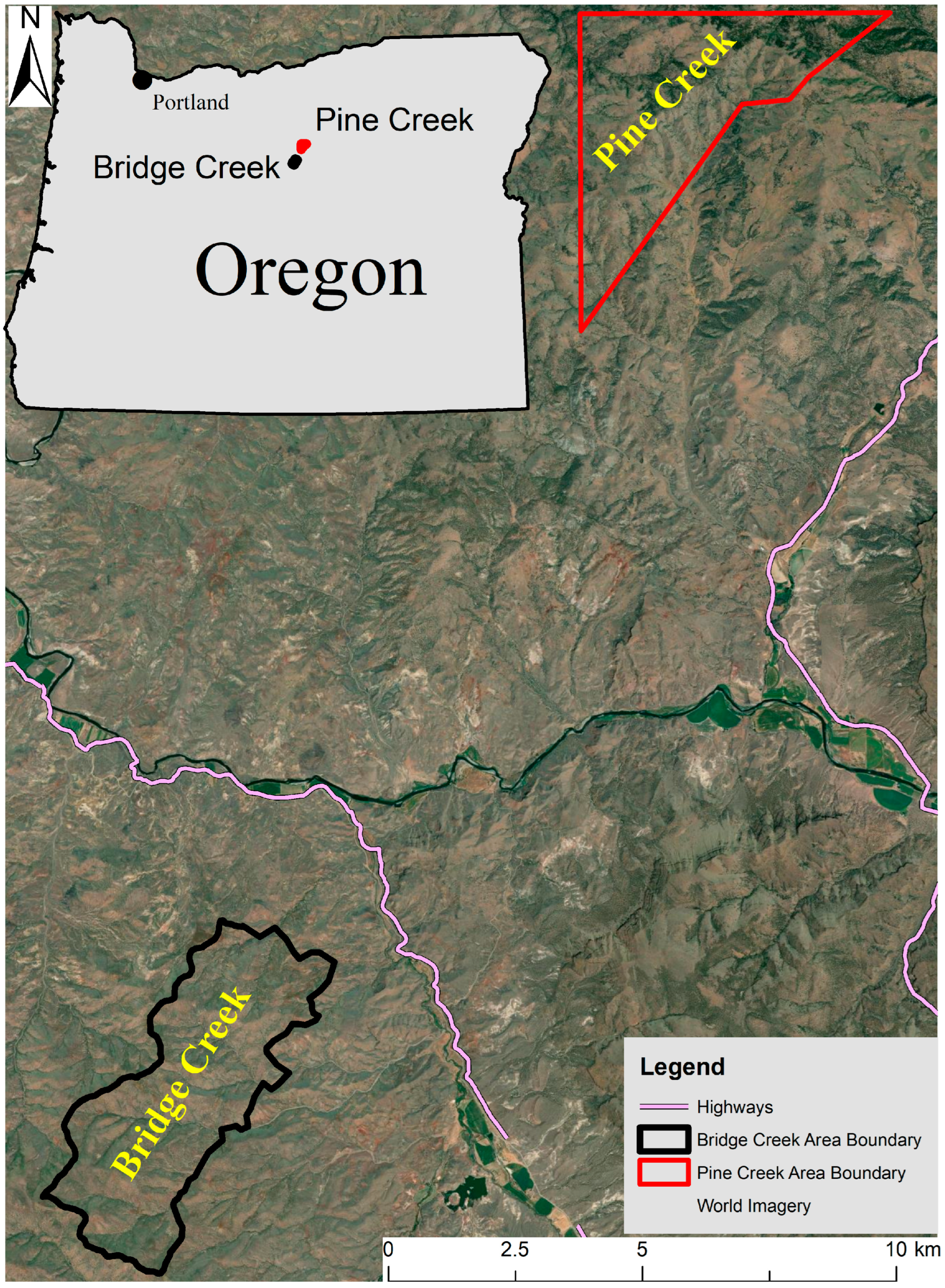
Figure 1. General location of the two study areas overlaid on orthorectified images produced by the National Agriculture Imagery Program. The latitude and longitude of the southernmost point of each area are presented in parentheses.
Sustainability 16 05124 g001
Figure 2. Road network and landings for the two study areas overlaid on the digital terrain model: (a) road network of the Bridge Creek area, (b) landings for the Bridge Creek Area, (c) road network of the Pine Creek area, (d) landings for the Pine Creek Area. The latitude and longitude of the northernmost point of each area are presented in parentheses.
Sustainability 16 05124 g002
Figure 3. Achievement of the optimal landscape restoration solution.
Sustainability 16 05124 g003
Figure 4. Improvement of the solution with the number of moves at 65 USD/ton (top 5 runs), with red being SA and black R2R: (a) Pine Creek area, (b) Bridge Creek area.
Sustainability 16 05124 g004
Figure 5. Improvement of the solution with the number of moves at USD 45 per ton (top 5 runs), with red being SA and black R2R: (a) Pine Creek area, (b) Bridge Creek area. The horizontal lines show the solutions trapped in a local maximum.
Sustainability 16 05124 g005
Table 1. Summary statistics describing the two areas.
Study AreaSurfaceElevation
Mean/Min ↔ Max/Std. Dev.
Roads LengthNumber of Sub-Basins
[ha][m][km][count]
Bridge Creek1667.9950/642 ↔ 1259/178.421.9 12
Pine Creek1597.11133/833 ↔ 1358/95.719.414
Table 2. Summary statistics for the predicted tree height and value.
Study AreaNumber of TreesHeight
Mean/Min–Max/Std. Dev.
[count][m]
Pine Creek178,5158.3/1.8–36.3/4.48
Bridge Creek162,9415.8/1.8–24.4/2.53
Table 3. Summary statistics for the possible landings. The average area per landing was calculated as the study area divided by the number of potential landings.
Study AreaNo. Potential LandingsAverage Area/Potential Landing [ha]
Bridge Creek3444.8
Pine Creek3994.0
Table 5. Summary statistics for the harvest value of 65 USD/ton.
Study AreaAlgorithmUpper BoundLower BoundMaximum
Net Revenue
Number of Solutions above/below
Lower Bound
Terminating Criteria for Best Solution
Bridge CreekSAUSD 289,752USD 117,752USD 154,94323/6freezing
R2RUSD 289,752USD 117,752USD 125,46423/6non-improvement
Pine Creek SAUSD 559,281USD 359,781USD 397,21912/17freezing
R2RUSD 559,281USD 359,781USD 365,83619/10non-improvement
Table 6. Summary statistics of the best solution for each area and algorithm for 65 USD/green ton value at the landing.
Study AreaHeuristicNumber of LandingsAverage Weight/LandingAverage Distance from Cell to LandingAverage Number of Cells/LandingAverage Number of Trees Harvested/LandingNet Revenue at Landing
[count][ton][m][count][count][USD/Merchantable Green ton]
Bridge CreekSA2239071.1942287.72/ton
R2R3086565.2682016.27/ton
Pine Creek SA26114771.98627610.35/ton
R2R35410868.3632039.56/ton
Table 7. Summary statistics for the best solution at a harvest value at the landing of 45 USD/green ton.
Study AreaAlgorithmUpper BoundLower Bound Maximum Net RevenueNumber of Solutions above/below Lower BoundTerminating Criteria of Best Solution
Bridge CreekSAUSD 9861−USD 162,139−USD 46110/0Freezing
R2RUSD 9861−USD 162,139−USD 48610/0Non-improving
Pine Creek SAUSD 37,049−USD 162,451USD 17,46810/0Freezing
R2RUSD 37,049−USD 162,451USD 17,31510/0Freezing
Disclaimer/Publisher’s Note: The statements, opinions and data contained in all publications are solely those of the individual author(s) and contributor(s) and not of MDPI and/or the editor(s). MDPI and/or the editor(s) disclaim responsibility for any injury to people or property resulting from any ideas, methods, instructions or products referred to in the content.