Abstract
Monitoring soil organic carbon (SOC) is essential for assessing the sustainability of soil usage. This study explores the spatial variability and mapping of SOC in Lithuania’s Nevėžis Plain using various interpolation methods, with an emphasis on understanding the impacts of soil typological units, moisture regimes, and erosion on SOC distribution. A total of 275 soil samples were collected from agricultural croplands at depths of 0–10 cm, supplemented by 38 samples from previous studies. The SOC map was created based on the contours of the Lithuanian soil geodatabase. Statistical analysis revealed that the distribution of SOC in the studied area was significantly influenced by soil moisture and the degree of erosion. Based on these findings, SOC mapping was conducted according to the contours of Lithuanian soils. Comparing the interpolation methods that were analyzed, it was found that the kriging, RBF, and EBK methods fail to adequately capture the minimum and maximum values of SOC, while the IDW fails to adequately capture only the minimum values. In summary, the integrated geographical approach is complex but applicable to SOC mapping. This method facilitates the creation of adaptable SOC maps that are both geographically and pedologically informed. Key principles to apply this approach for future research and practical application should include establishing a statistically reliable data foundation, categorizing samples based on contrasting soil moisture regime, degrees of erosion, and land use patterns, and developing contouring principles along with a criteria algorithm that enables accurate spatial interpolation of average SOC values.
1. Introduction
The spatial variability of soil organic carbon (SOC) is an important indicator that shows not only the conditions of pedogenesis and its nutrition but also the intensity of its use in the context of sustainability [1]. In the context of climate change, SOC spatial research and mapping using GIS tools are particularly relevant for assessing the sustainability of agricultural activities and their impact on SOC sequestration. Revealing the characteristics of SOC’s spatial pattern of SOC will provide a basis for evaluating soil fertility and assist in the development of sound environmental management policies for agriculture [2]. Accurate accounting of the amount of SOC in the soil and modeling and forecasting its changes are important for sustainable development in agroecosystems.
The initial mapping of soil cover across Lithuania, conducted on a coarse scale, took place between 1953 and 1969 [3] and relied on field data for its foundation. Subsequent adjustments to the soil contours were made between 1970 and 1991, incorporating new field data to refine the mapping accuracy [3]. The activities included mapping soil typological units according to the Lithuanian genetic classification and identifying the degree of erosion of the topsoil layer by its thickness and color. The mapping was based on the principle of distinguishing elementary surfaces and taking soil samples from each of them. They were later analyzed in the laboratory to determine the exact soil typological unit. At the end of the 20th century, this method was developed using orthography and distinguishing the surfaces to be mapped according to the typical colors of the cultivated surfaces of the fields using RGB sensors with a visible spectrum.
In 1999, the National Genetic Soil Classification (TDV-96) was transformed into the Diagnostic Soil Classification of Lithuania (LTDK-99), aligned with the 1998 World Reference Base for Soil Resources. In Lithuania, the LTDK-99 classification is still in use [4] and does not conflict with the currently used WRB 2022 classification [5]. It is easily adaptable because it is based on the same soil classification principles.
The soil mapping efforts previously conducted laid the foundation for the creation of Lithuania’s GIS soil database (Dirv_DR10LT) in 2012, which was revised in 2014. This soil database has become the basis for contemporary detailed spatial studies of Lithuanian soils. In total, the Dirv_DR10LT contains 1,482,754 soil contours, with the minimum contour size being 0.01 ha and the average size of a contour being 4.4 ha. The Dirv_DR10LT [6] database was constructed using 101,146 soil profiles, which are distributed throughout the country. This database is accessible at https://www.geoportal.lt/geoportal (accessed on 25 January 2023). These data provide an important basis for the development of geospatial-based detailed mapping techniques and contouring principles.
This database is periodically updated; for instance, in 2023, the SOC data (12,000) points collected in 1985–1991 in different local Lithuanian regions and analyzed in the laboratory were digitized. These were used to create a GIS database (DirvAgroch_DR10LT) [7]. In 2016, the SOC data from 752 points [8] for the entire Lithuanian territory were collected following Land Use, Land-Use Change, and Forestry (LULUCF) grid points, and 383 points were collected following the Land Use and Coverage Area frame. While these databases cover the entire country well, the methods used by data collectors in gathering samples varied, which means they do not fully meet the criteria of data representativeness that underpin this study. Additionally, the possibility of conducting statistical analysis on these data in the context of soil moisture and erosion degree is also limited.
The older databases of soil samples collected by traditional methods and the rapid development of remote sensing technologies have made it possible to extend the boundaries of SOC mapping [9] and to make the process partly automated. If it is required, the mapping process now includes satellite data, multispectral or hyperspectral imagery from unmanned aerial vehicles, proximal sensors, and machine learning models. Despite the wide choice of remote-sensing methods, the reliability of the results remains an important issue [9]. Therefore, this study raises the debate on combining modern and classical methods to find the optimal method for SOC spatial research.
This study is relevant as it diverges from the mainstream focus on identifying the optimal interpolation method and its parameters, sample optimization, and the application of remote sensing technologies and machine learning tools [10,11,12]. Instead, recognizing the heterogeneous nature of soil cover, we seek to adapt classical mapping methods to the contours of soil typological units and the information they encapsulate. This approach aims to enhance not only data sampling but also the precision of mapping, with a particular emphasis on highlighting extreme azonal SOC values.
Grassland remains one of the main challenges when mapping SOC in agricultural areas. The application of remote sensing techniques on these surfaces [13], which are never fully bare, is a relevant but challenging process due to issues with interpolation accuracy. Typically, the question of SOC content in grasslands is addressed using derivative indices [13].
Currently, various technologies are used to predict SOC distribution at local, regional, and national scales. These mostly include statistical and geostatistical approaches, satellite images, or interpolation methods required for GIS data analysis.
Several studies have demonstrated that integrating field measurements with kriging interpolation and GIS methods enables the production of contour maps showing the distribution of soil texture, soil organic carbon (SOC), and the carbon/nitrogen (C/N) ratio [14]. Furthermore, Bhunia et al. [2] compared five interpolation methods to generate spatial distribution maps of SOC: inverse distance weighting (IDW), local polynomial interpolation (LPI), radial basis function (RBF), ordinary kriging (OK), and empirical Bayesian kriging (EBK). This comparison revealed that the OK interpolation method is superior to other geostatistical and deterministic methods for predicting SOC across relatively large geographical areas. In our study, we also applied these interpolation methods but critically assessed their application based on the assumption that the young geological age of our study area, characterized by complex relief and a high diversity of soil-forming deposits, could limit accuracy.
In a different approach, Castaldi et al. [15] explored the feasibility of using Sentinel-2-based approaches for high-resolution mapping of SOC and clay in cropland sites with varied climates and soil types. The results indicate that the accuracy level and uncertainties were primarily influenced by site-specific soil characteristics and soil management practices. However, the overall performance of the models was reasonably accurate at most sites. These findings highlight the potential of combining advanced remote-sensing techniques and geostatistical methods to improve soil-property mapping, which is essential for effective land management and agricultural practices.
The use of standard interpolation methods for mapping (as well as SOC) is predicated on the assumption that the space for modeling is uniformly homogeneous and unaffected by various environmental components and factors [16]. Meanwhile, soil coverage is inherently heterogeneous and influenced by a mix of zonal and azonal factors, both natural and anthropogenic. This heterogeneity suggests that interpolation methods are favorable and suitable to local areas with uniform characteristics. Interpolation methods are also suitable for large areas where soil cover is formed by dominant zonal soil-forming processes. This is complicated for the Lithuanian territory and regional level in the context of SOC mapping, where soil complexity and diversity become more pronounced; alternative methodologies are necessary to accurately capture and represent the variability in SOC distributions.
The SOC levels in agricultural soils are determined by a multitude of factors, including land management practices, land use, soil texture, origin of soil-forming deposits, moisture content, relief, and type of vegetation cover [17,18]. Additionally, variations in SOC amounts are linked to soil cultivation methods, especially in practices devoid of agrochemical inputs [19,20]. Our study specifically examined how SOC content correlates with soil type and moisture regimes. This approach mirrors similar research undertaken by other European scholars [8,21,22] who explored the relationship between SOC levels and soil typological units. For instance, research conducted in Estonia [22] has highlighted the impact of soil irrigation types and carbonation on SOC quantities. Given that Lithuanian soils develop under conditions closely resembling those in Estonia, it is hypothesized that factors such as moisture and soil typological units, including their carbonation levels, play crucial roles in shaping SOC distribution across Lithuanian agricultural lands.
Until recently, in Lithuania, there have been no efforts to synthesize the average SOC content across different typological and soil groups (by classification level, moisture regime, and degree of erosion) into broader geographical generalizations. This includes the absence of initiatives to create comprehensive SOC maps or undertake spatial analyses based on these values.
To address these challenges, we aim to demonstrate an integrated geographical approach (IGA) for detailed SOC mapping. This involves combining GIS and traditional research methods to achieve a highly accurate SOC map at both the local and regional scales. It also addresses the issue of contouring of different SOC contents and the distribution of SOC in the area determined by zonal and azonal soil-forming processes.
The objectives of this study are as follows: (1) to compile a representative collection of soil samples that reflects the soil-forming conditions of the Nevėžis Plain territory, taking into account the typological units of the soil; (2) decomposition of the name of the territorial unit of the soil according to the groups of the first level of the soil and the nature and degree of their wetting; (3) establishing the relationship between SOC and the decomposed parts of the soil typological unit in addition to considering the degree of soil erosion; (4) to develop a soil organic carbon concentration map for the Nevėžis Plain territory.
This plain accounts for about 15% of the total area of moraine plains in Lithuania but represents the most typical of them, the absolute majority of which (about 95%) are localized in the Central Lowlands of Lithuania. They are dominated by morainic sandy loams typical of these plains. Therefore, the results of this study can be interpolated to almost 38% of the territory of Lithuania.
2. Materials and Methods
2.1. Study Area
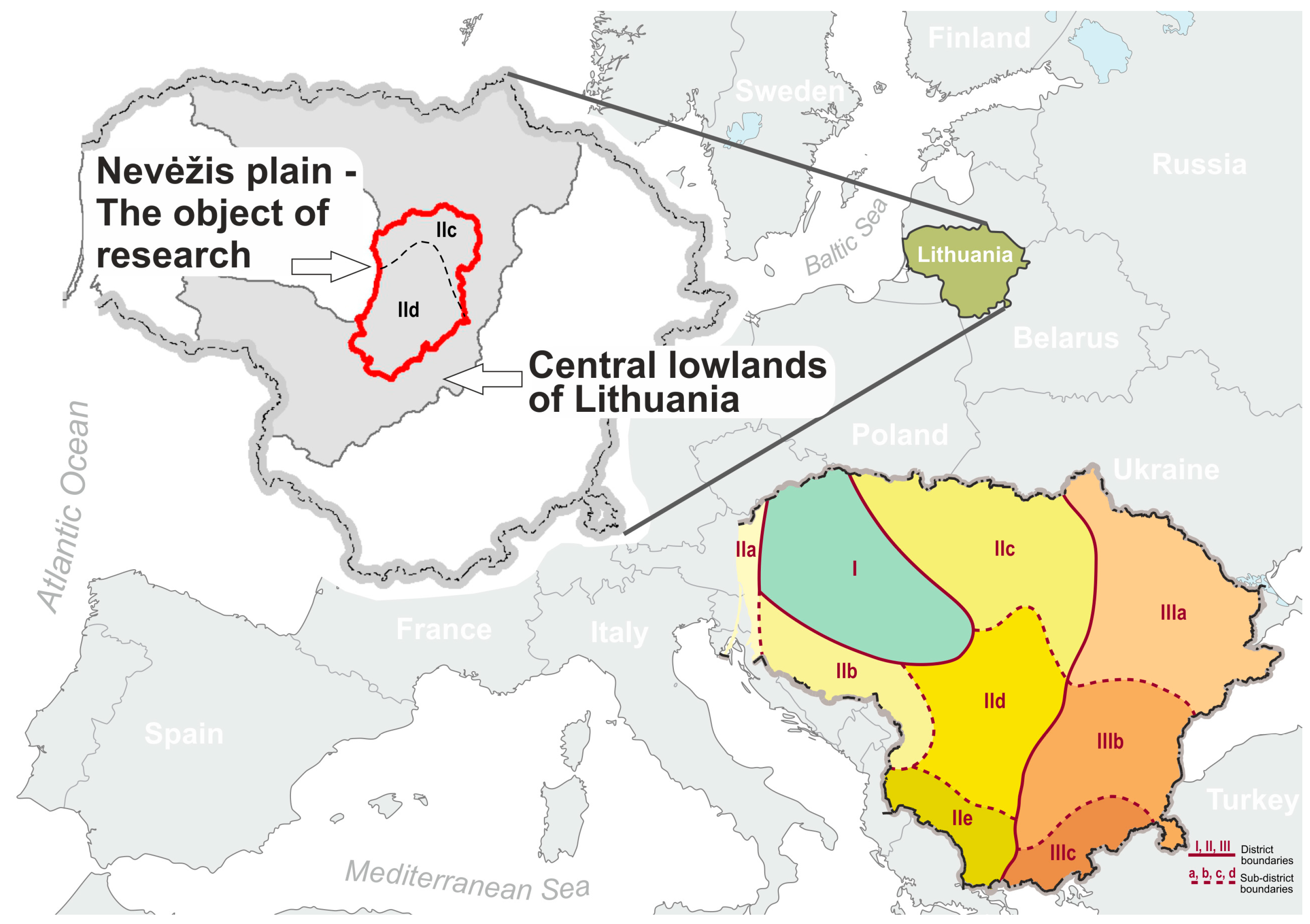
The study area is situated in the central part of Lithuania between 55°40′–54°57′ N and 23°45′–24°31′ E (Figure 1). The selected research area covers the geomorphological district of the Nevėžis moraine plain (430,826.64 ha) in the lowlands of Central Lithuania between the city of Panevėžys in the north and the city of Kaunas in the south.
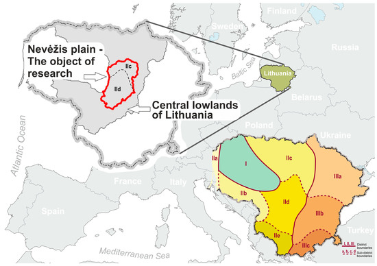
Figure 1.
The contours of the object of research—Nevėžis Plain location—are marked with a red line. The gray background represents the central lowlands of Lithuania. The map on the right shows the different agroclimatic regions of Lithuania (I—uplands region of western Lithuania, II—lowlands region of central and western Lithuania (IIa, IIb, IIc, IId, IIe), III—uplands region of eastern Lithuania (IIIa, IIIb, IIIc).
According to the “Environmental Stratification of Europe”, the area of study falls within the Nemoral climate zone, which is characterized as continental and cool, with a relatively short growing season for plants [23,24]. The southeastern territories of Estonia and Latvia, along with the northwestern regions of Belarus, are also classified under this climate zone. According to the agro-climatic classification of Lithuania [25], the study area falls within two agroclimatic zones: IIC and IID (Table 1).

Table 1.
Agro-climatic indicators of the studied area [25].
The surface of this Nevėžis Plain was formed 13,000–14,000 years ago [26,27] in the ground moraine deposits by the deglaciation of the Middle Lithuania phase of the Late Nemunas (corresponding to the Late Weichselian glacier in Europe) glaciation. Marginal morainic loam and fluvioglacial sand formations are common only at the edges of the territory, which borders other geomorphological units.
Nevėžis moraine plain is characterized by a flat/wavy surface and ground moraine carbonate loam soil-forming rocks [28]. Some of the most fertile soils in Lithuania are spread in this location, where even 68.45% of the territory is used for agricultural purposes, while the remainder, that is, 31.55%, is classified as forests, water bodies, or built-up areas.
According to the 2023 data from the Official Statistics Portal [29], in the agricultural area analyzed, cereals (54.35%) and rapeseed (17.77%) predominated, while protein crops accounted for only 5.59% of the total number of crops grown. All other crops accounted for 13.55% of the total area. Permanent grasslands and pastures accounted for only 8.74% of the total. A more detailed distribution of the plants is presented in Table 2.
Table 2.
Distribution of agricultural crops in the Nevėžis Plain territory in 2023 [29].
The studied area is characterized by the fact that carbonates in soils are leached to an average depth of 40–60 cm. Owing to the prevailing soil decarbonatization and lessivage processes, the dominant soil texture in the topsoil layer was sandy loam, which accounted for approximately 83.73% (Table 3), whereas in the lower soil layers, the dominant soil texture classes were sandy loam (61.34%) and loam (21.16%). According to LTDK-99 classification, the main soils in Nevėžis moraine plain are cambisols, gleysols, and luvisols, and they cover 49.63, 21.03 and 17.64%, respectively (Table S1). In addition, it is important to note that the aforementioned soils have varying degrees of waterlogging (from gleyic to muck and peat gley). Soils of other typological groups (arenosols, histosols, fluvisols, planosols, regosols, retisols, podzols, and leptosols) accounted for only 11.7% of the total agricultural land. Peatland surfaces, which were mostly covered with forest, accounted for approximately 3% of the analyzed area. Most of the soils in the area were characterized as semi-hydromorphic (76.66%) or hydromorphic (3.04%) (Table S1).
Table 3.
Distribution of the number of collected samples in the study area according to texture classes.
2.2. Soil Description and Sampling
Soil samples were collected from the Nevėžis moraine plain (area—4308.27 ha) in October 2021 and May 2022. During 8 field campaigns, 275 soil samples were collected from agricultural croplands and from the topsoil layer at a depth of 0–10 cm. Each sample consisted of three to four sub-samples taken within an area of 1 m in radius. In this area, the sampling density was 0.08 per km2. Soil sampling points were selected using a Lithuanian soil typological map, the scale of which was 1:10,000 [6]. In this map, soils are identified using Lithuanian LTDK-99 soil classification [4]. However, it is important to note that this LTDK-99 classification accurately reflects FAO principles. In further parts of this paper, summaries of already converted (from the LTDK-99 classification to WRB 2022) soil typological units are used. Sampling point coordinates were found with an accuracy of 1–2 m using a GPS receiver (Trimble Juno T41/5) with ArcPad 10.2 software (ESRI).
Additionally, we used SOC data collected from previous studies covering the Lithuanian National Forest Inventory [25,26]. In this study, 754 samples were collected at the national level, but we selected only part of the data that fell within the Nevėžis moraine plain area, and we selected only those points that were collected from cropland; thus, we were able to use 38 soil samples [25,26] in our study. The basic statistics for SOC under different types of soils are given in Table S1, and information about soil texture classes is presented in Table 3.
Table S1 shows the complete data set used in the study. The research represents 79.1% of the studied area, i.e., agricultural land, and, respectively, 99.99% of all soil diversity in this territory (according to the first classification level). According to the second classification level, the representativeness reaches 99.78%. All types of soil moisture regimes are also fully represented. On average, 1 sample/200 ha was taken in the studied area. However, this assessment is relative since the number of points in different soil typological units at different levels is very different. Although the density of points in the dominant soil groups (CM, GL, LV) and moisture classes (SH(g8), SH(G), AU) is one of the lowest, the absolute sample of points is the largest (Table S1). These differences arise because the sampling points were formed to achieve as even a distribution as possible in the territory and to represent the diversity of the soil cover.
Most samples (229 points) were taken from soils whose topsoil was dominated by sandy loam (Table 3). Since the research area is plain and its soil cover structure is dominated by waterlogged soils, much attention was paid to mucky and peat soils. They contained 19 and 24 samples, respectively. The average density of sample points was about 0.17 units/100 ha, or 1–2 units/1000 ha.
2.3. Chemical Analyses
During the laboratory analyses, the visible roots and plant residues were first removed manually, and then the soil samples were air-dried, crushed, sieved through a 2 mm sieve, and homogeneously mixed. For SOC analysis, the samples were passed through a 0.25 mm sieve. SOC content was determined by a photometric procedure at a wavelength of 590 nm using a UV–VIS spectrophotometer Cary (Varian) and glucose as a standard after wet combustion according to the Tyurin method modified by Nikitin [30]. All chemical analyses were conducted at the Chemical Research Laboratory of the Lithuanian Research Centre for Agriculture and Forestry.
2.4. Data Preparation and Mapping
The SOC map was compiled based on the contours of the Lithuanian soil GIS database (Dirv_DR10LT-1554, 2022, scale 1:10,000) [6] (Figure 2). A total of 275 samples from the study area’s agricultural soil cover were collected during the field trip, and 38 points from the official scientific report on which the publication was based [8,31] were used. In total, 313 points were used to create the map. The sample of soil samples is formed in such a way that it represents the variety of soil typological units according to the soil typological group, moisture regime, and degree of moisture prevailing in Lithuania. Anthrosols and Leptosols were not used in the mapping because Leptosols are not identified in the studied area, and Athrosols are identified in urbanized areas that were not mapped during this study. Samples were taken only from agricultural land that was not covered with vegetation, choosing the location of the point in such a way that it was at least 100 m away from roads, forests, or other lands.
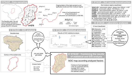
Figure 2.
Methodological diagram of SOC mapping.
During the analysis, each soil sample was related to the name of the soil typological unit based on the soil contours of the Dirv_DR10LT database [6] and the refinement of their position in the area. In the next step, the name of the soil typological unit was deconstructed into the type of moisture regime and degree of moisture and belonging to the level I soil typological group (classifier is meant) (Figure 2). Three scenarios of the IGA method were selected for analysis and mapping. In the case of the first scenario, average SOC values were calculated for soil typological units of level II. In the case of the second scenario, average SOC values were calculated by deconstructing soil typological unit indices of level II into soil moisture regime types. Finally, for the third scenario, average SOC values were calculated by additionally evaluating the degree of soil erosion. Based on these identifiers, a statistical analysis of the SOC data was performed, during which the reliability and statistical differences of the data were evaluated.
To compare the results of the study, the collected SOC data were used for SOC mapping using different interpolation methods. The chosen interpolation methods included those used in previous studies [2] and those that are easily applied within the ArcGIS spatial analysis platform: IDW, kriging, LPI, RBF, and EBK.
IDW (inverse distance weighting) is a method of weighted distance average, the value of which cannot exceed the highest or drop below the lowest input value [32].
Kriging is a method that assumes that the distance or direction between sample points reflects a spatial correlation that can be used to explain variation in the surface. The kriging tool fits a mathematical function to a specified number of points, or all points within a specified radius, to determine the output value for each location. [33].
The LPI (local polynomial interpolation) method applies to fit many polynomials, each within specified overlapping neighborhoods. The neighborhoods overlap, and the value used for each prediction is the value of the fitted polynomial at the center of the neighborhood [33].
The RBF (radial basis functions) method uses one of five basis functions to interpolate a surface that passes through the input points exactly. RBFs are used to produce smooth surfaces from a large number of data points [33].
EBK (empirical Bayesian kriging) is one of the geostatistical interpolation methods that, by accounting for error, generates the underlying semivariogram. This approach combines kriging with regression analysis to make predictions that are more accurate than either regression or kriging can achieve on their own [33].
2.5. Statistical Analysis
Statistical analysis was performed using SAS Enterprise software, version 7.1 (SAS Institute Inc., Cary, NC, USA). Differences among SOC samples were tested using two-way analysis of variance (ANOVA). The probability level was set at 0.05 and grouped according to letters by Duncan’s test. The statistical analysis was carried out according to the following factors: factor A—soil organic carbon (SOC); factor B—first-level soil typological groups, second-level soil typological groups, and soil moisture regime type. Standard error (SE), minimum (Min), and maximum (Max) values were used to estimate the deviations of soil parameters from the mean values.
The ANOVA analysis factors were selected to assess and compare the statistical reliability of the values grouped by socio–mental factors (soils classified according to conventional attributes, i.e., soil typological groups) and the values grouped according to the natural zonal and azonic factors (moisture regime and degree of erosion integrated into the moisture regime classes). The aim was to distinguish and assess the impact of subjective (human reasoning) and objective (natural conditions) factors on the obtained values and the statistical reliability of their correlations.
Calculated average values of SOC, according to moisture degree groups, were related to soil contours. It was considered that the studied area contains eroded soils characterized by different degrees of erosion (about 4% of the total contour area), and the SOC amount was corrected in the contours of eroded soils (Figure 2). The correction is based on empirical data showing that the amount of SOC in eroded soils cannot exceed 2% of SOC. The following data were used for the cartographic basis of the map: National Land Service under the Ministry of Agriculture of the Republic of Lithuania: GDB10LT-static-4825 2021-02-24, Dirv_DR10LT-1554 2021-02-24 [6,34].
3. Results
3.1. Comparison of the Application of Interpolation Methods
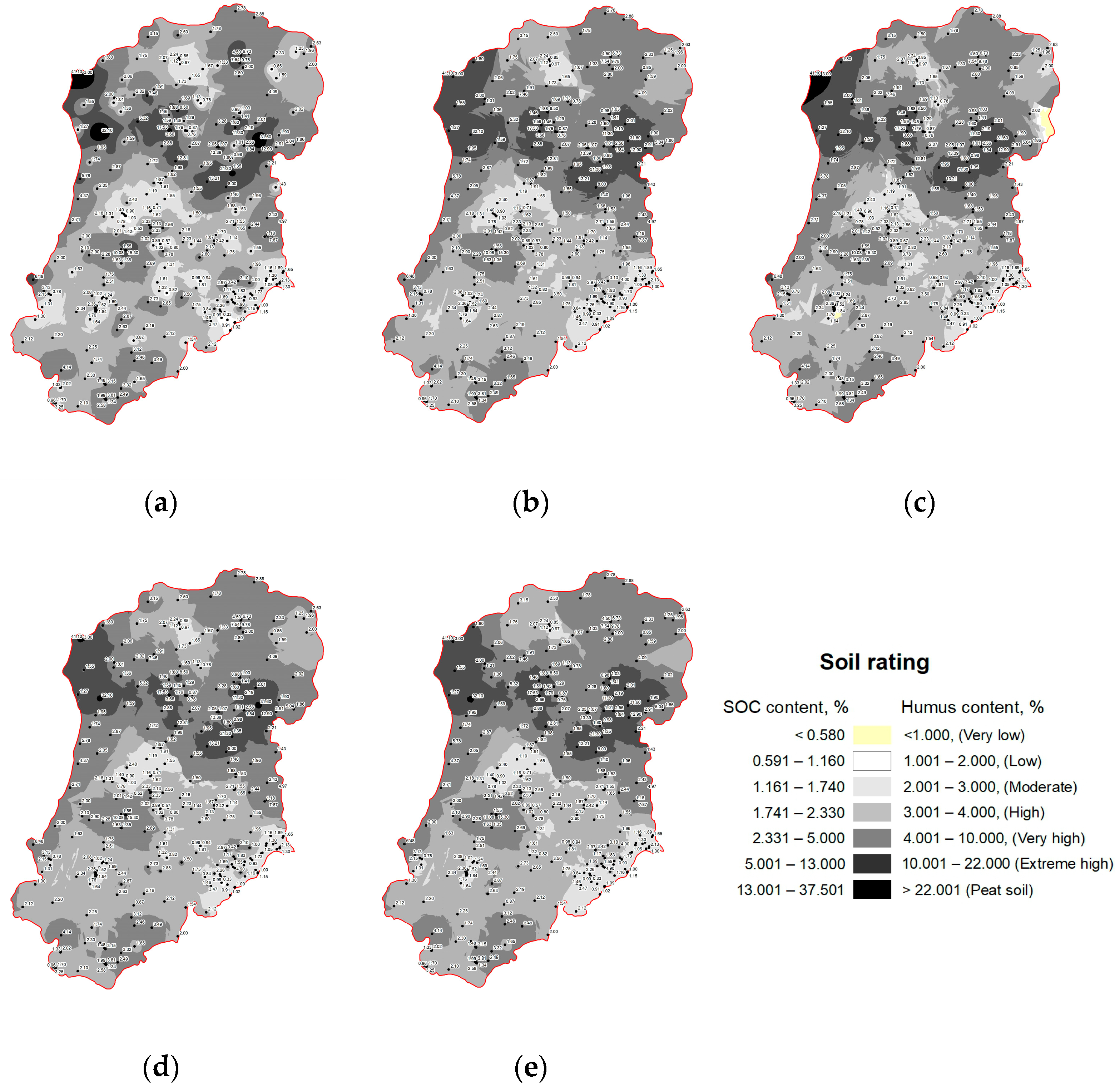
The comparative analysis of different interpolation methods (Figure 3, Table 4) showed that there are no essential differences between these methods, and they all operate on the principle of leveling values. None of the methods distinguished one dominant group of SOC values, although from the data of the analyzed area discussed above (Table S1 and Table 3), it is demonstrated in Table 3 sandy loam texture class and Cambisols soil typological group dominate in the studied area. Basically, the values of cells (10 × 10 m) are mostly concentrated in two SOC groups—high (1.741–2.330) corresponding ≈ one-third or 36.6–38.7%, while the very high (2.331–5.000) group is even larger, i.e., 37.82–42.85% of the total area (Table 4). It should also be noted that the results of the analyzed interpolation methods differ slightly in their extremes, i.e., distribution of low/very low and extreme high/peat soil SOC values.
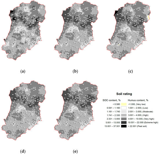
Figure 3.
SOC mapping (with the accuracy of 10 × 10 m cells) using the inverse distance weight (IDW) (a), kriging (b), local polynomial interpolation (LPI) (c), radial basis functions (RBF) (d), and empirical Bayesian kriging (EBK) (e) methods.
Table 4.
Spatial distribution of soils in the Nevėžis Plain by SOC content using different interpolation methods for calculating the average SOC value.
Kriging, LPI, RBF, and EBK methods practically eliminate SOC values that are assigned to the peat soil group (SOC > 13%). There are also very low and low values (<0.580−1.16%), which should be associated with eroded soils. Only the interpolation performed by the IDW method managed to show a relatively high percentage of SOC values: very low and low—1.00%, peat soil—1.17%. Nevertheless, these values are still considerably lower than the areas of eroded soil (1.65%) and peat soil (3.04%) isolated in this area.
3.2. Results of the Application of the Integrated Geographical Approach Method
In the conducted research, the problem of spatial discretization—the question of the unevenness of the soil cover properties—is solved using a data layer of contours of typological units of the soil cover. The average values typical for a specific soil typological unit (according to genesis, type of irrigation, and erosion) were measured in field conditions and calculated during statistical analysis.
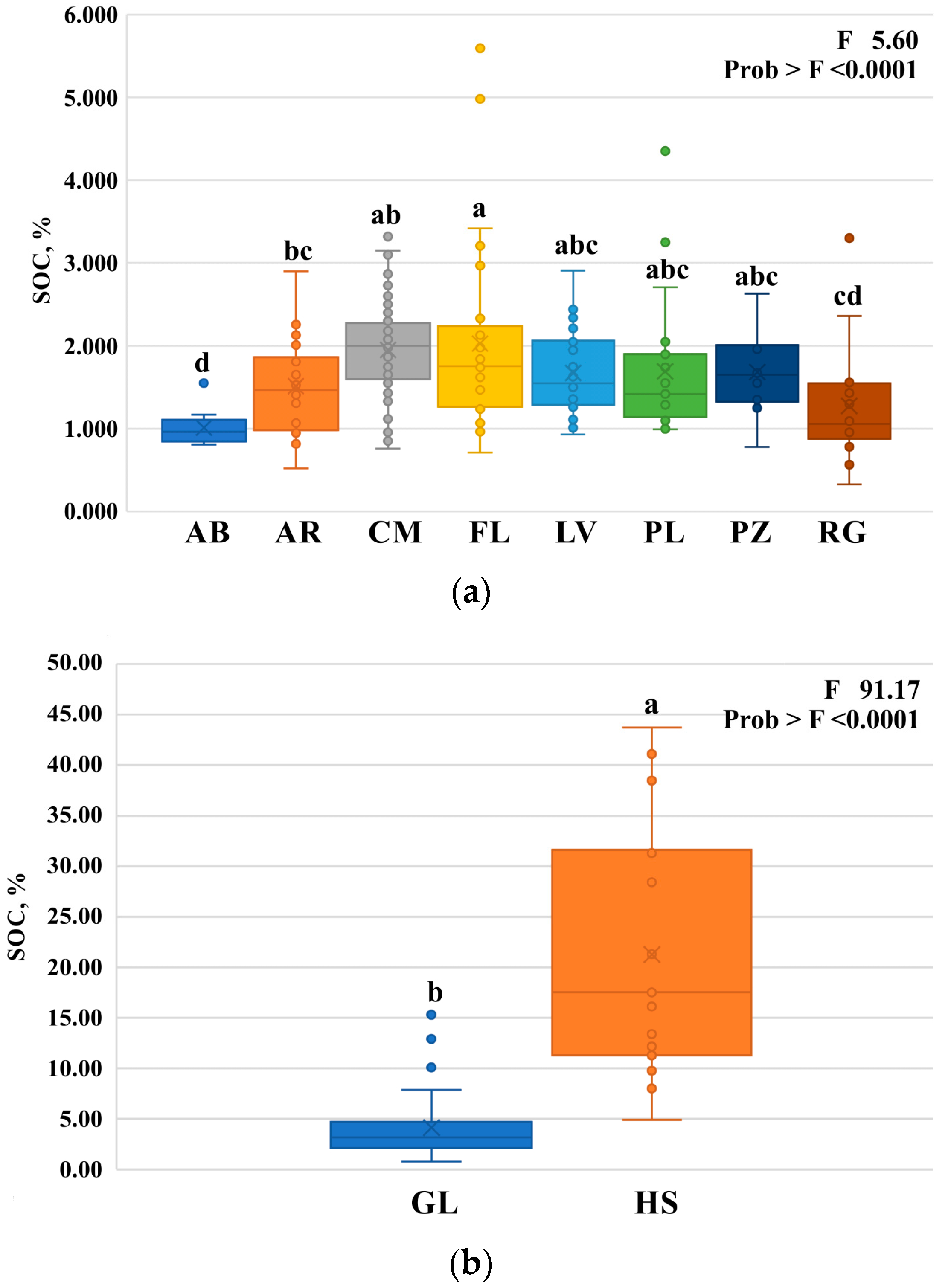
Statistical analysis showed that the classification of mineral soils into specific typological groups (the assignment was made according to the Lithuanian soil classification (LTDK-99) [4]) and evaluation in terms of SOC values show statistically significant differences between some soil groups. The order is as follows: for mineral soils: FL > CM ≈ LV ≈ PL ≈ PZ > AR > RG ≈ AB; for organic soils: HS > GL (Figure 4a). These differences can be explained by their different origins. Albeluvisols (AB) formed in marginal moraine deposits, Arenosols (AR) in sandy deposits, Cambisols (CM) in ground moraine deposits, Fluvisols (FL) in alluvial sandy deposits, and Regosols (RG) formed due to severe erosion. Luvisols (LV), Planosols (PL), and Podzols (PZ) also differ in origin. However, the results of the study in terms of SOC content partially show statistically significant differences in these soil groups.

Figure 4.
Box plots illustrate the content of SOC in different groups of soils: (a)—mineral soils and (b)—organomineral and organic soils. Box boundaries indicate the 25th and 75th percentiles and whiskers below and above indicate minimum and maximum values, excluding outliers. RG—Regosols, AB—Albeluvisols, FL—Fluvisols, LV—Luvisols, AR—Arenosols, CM—Cambisols, PL—Planosols, PZ—Podzols, GL—Gleysols, HS—Histosols. a–d letters in the figures indicate a statistically significant difference at p < 0.05.
However, we can see that more organic carbon is found in Cambisols, Fluvisols, Podzols, and Gleysols (Figure 4a,b). Such results contradict the principle that more productive soils must have more SOC because out of these groups, only Cambisols are productive, while other groups in Lithuania are classified as less productive soils. Moreover, these results can be explained by the fact that in these groups of mineral soils, in the analyzed area (moraine loam plain), partly waterlogged gley soils predominate.
Of course, certain assumptions can be made regarding the differences in the average SOC values of individual soil typological groups. Luvisols (LV), arenosols (AR), and fluvisols (FL) in the studied area, according to the research data, are characterized by a relatively lower amount of SOC. This is due to lower moisture content (LV) and sandy texture (AR and FL). Cambisols (CM) are the most productive predominant soils of the region. The analyzed SOC research data supports this. Relatively higher values of SOC (Figure 4a,b) in cambisols are determined by the prevailing loamy texture and excess moisture—gley or stagnic properties.
The presence of outlier point values (Figure 4a,b) in the samples of soil groups is not a measurement or experiment error. These SOC values indicate a large heterogeneity of soil typological groups that can be related to moisture regime and degree of waterlogging, erosion level, and other factors. This presupposes that the grouping and averaging of SOC data by first-level soil typological groups is not correct in the context of SOC mapping. Therefore, the simulation of the average SOC values was carried out by sequentially applying the IGA method according to three different scenarios (Figure 2), the results of which are presented in Table 5.
Table 5.
Spatial distribution of agricultural soils by SOC content using different scenarios of integrated geographical approach (IGA) for calculating the average SOC value.
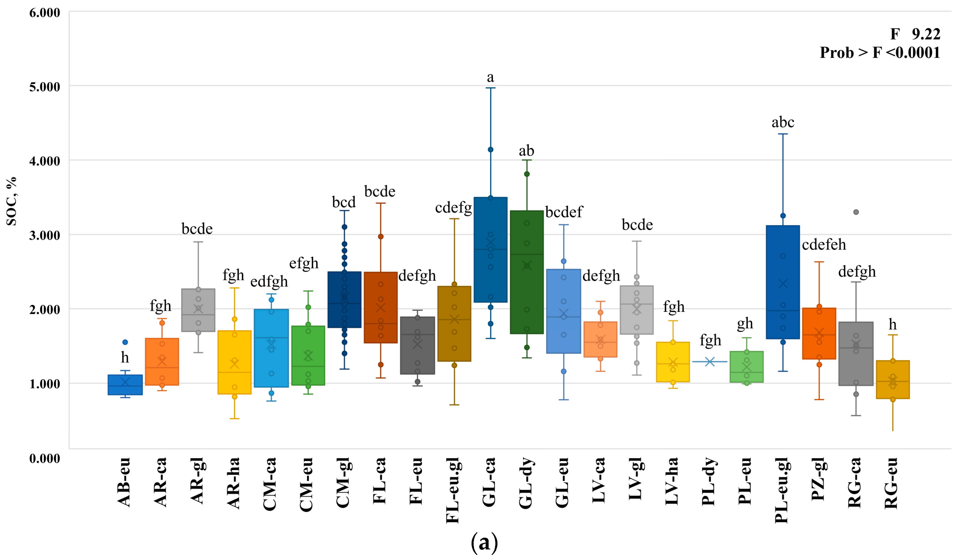
The analysis shows (Table 5) that when grouping SOC data according to different criteria, different results are obtained. Very interesting results were obtained by grouping SOC values according to soil typological units of classification level II (scenario I) (Figure 5a,b, Table 3). In most cases, a statistically significant difference was found in the degree of base saturation (dy, ha, eu, and ca) and the degree of waterlogging (non, gl) for the soil typological units, which differ from each other according to the predominant soil-forming process and soil-forming deposits (first-level soil group index).
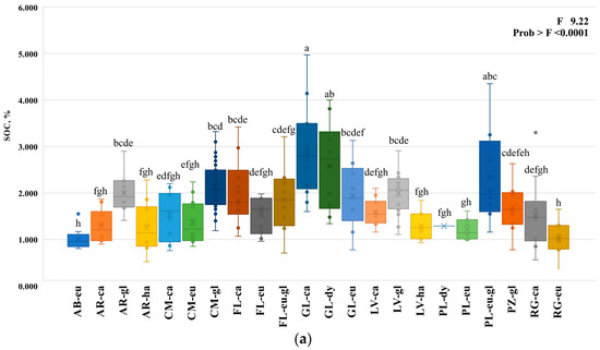
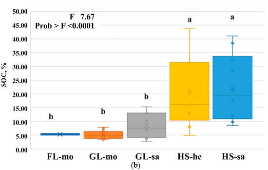
Figure 5.
Soil organic carbon content according to soil typological units of level II: (a)—mineral soils, (b)—organomineral and organic soils. Box boundaries indicate the 25th and 75th percentiles and whiskers below and above indicate minimum and maximum values, excluding outliers. FL-eu—Eutric Fluvisol, GL-eu—Eutric Gleysol, GL-sa—Sapric Gleysol, GL-ca—Calcaric Gleysol, GL-dy—Dystric Gleysol, GL-mo—Mollic Gleysol, LV-gl—Gleyic Luvisol, LV-ca—Calcaric Luvisol, LV-ha—Haplic Luvisol, PZ-gl—Gleyic Podzol, HS-sa—Sapric Histosol, PL-eu—Eutric Planosol, PL-eu.gl—Gleyic Eutric Planosol, CM-gl—Gleyic Cambisol, CM-ca—Calcaric Cambisol, AR-gl—Gleyic Arenosol, AR-ca—Calcaric Arenosol, AR-ha—Haplic Arenosol. a–h letters in the figures indicate a statistically significant difference at p < 0.05.
Such results were obtained because the distribution of SOC in the soil is mostly determined by natural (ecological) and human economic activity (socioeconomic) factors. Meanwhile, the classification of soils into groups is considered a social/psychological factor. Soils are grouped into groups according to agreed criteria that essentially summarize the characteristics of soil formation. Characteristics and criteria such as humidity are transferred to the second (e.g., CM-gl, AR-gl, etc.) and, in individual cases, to the third level of classification (e.g., FL-eu.gl, PL-eu.gl) (Figure 5a,b).
Interpretation of these results is difficult. Although the results show (Figure 5a,b, Table 3) that carbonate soils (-ca) have more SOC (1.587%) compared to non-carbonate soils (-ha, -eu, and -dy) (1.229–1.290%) and statistically, in this case, the differences between individual soil groups are reliable in most cases, there are exceptions. These are AR-eu, AR-ha, LV-ha, PL-dy, FL-eu, LV-ca, and RG-ca. This shows that soil moisture, texture, degree of erosion, and other factors play a significant role in determining the amount of SOC in the soil. Basically, the available results illustrated in Figure 5 show that each soil group (according to the second classification level) is unique. This presupposes that when evaluating the amount of SOC in the soil cover according to this principle, each soil group must be evaluated.
The grouping and averaging of SOC values according to the nature of the soil moisture regime (scenario II) (Table 5 and Figure 6a,b) shows that the SOC values are redistributed in relation to the moderate and high SOC content groups. The change occurs because individual soil typological groups (due to the geographical peculiarities of their formation) are characterized by a different ratio between automorphic and semi-hydromorphic moisture regime subgroups, so the grouping of SOC data by soil typological units eliminates these differences. Meanwhile, grouping according to the nature of the moisture regime highlights one of the essential factors determining the amount of SOC—the type of moisture regime and its amount in the soil. After adjusting the SOC values according to the soil erosion factor (scenario III), groups of very low and low SOC values appear (Table 5). They are formed at the expense of the moderate group of SOC values since the data of this group are mainly formed by the data sample belonging to soils of the automorphic moisture regime.
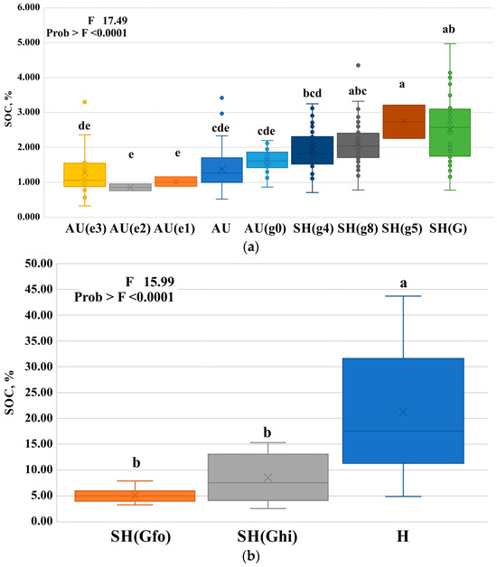
Figure 6.
Soil organic carbon content by type of soil moisture regime: (a)—types of moisture regime leading to humification or mineralization of soil organic matter, (b)—types of moisture regime leading to the process of peat formation in the soil. Box boundaries indicate the 25th and 75th percentiles and whiskers below and above indicate minimum and maximum values, excluding outliers. AU—automorphic (gleyic, deeper than 200 cm), AU(g0)—automorphic (gleyic, 100–200 cm), SH(g4)—semi-hydromorphic (gleyic, 50–100 cm), SH(g8)—semi-hydromorphic (gleyic, up to 50 cm), SH(g5)—semi-hydromorphic (gley, 50–100 cm), SH(G)—semi-hydromorphic (gley, up to 50 cm), SH(Gfo)—semi-hydromorphic (folic, gley, up to 50 cm), SH(Ghi)—semi-hydromorphic (histic, gley, up to 50 cm), H—hydromorphic (Histosols), e1—weakly eroded, e2—moderately eroded, e3—severely eroded. a–e letters in the figures indicate a statistically significant difference at p < 0.05.
The data analysis shows that the more objective SOC values for mapping and modeling of SOC content in the soil cover are those collected and calculated based on primary natural soil properties (such as moisture and soil erosion) (Figure 6a,b) rather than those resulting from soil classification and generalization. The grouping of soils according to the moisture regime and their erodibility to map the amount of SOC contained is less affected by subjective factors than the typification by the genetic groups of soils (according to national or international classifications). The validity of the choice of moisture regime and soil erodibility criteria is also confirmed by studies conducted in Estonia [22]. The same regularities of SOC distribution were found in these studies. SOC distribution is ambiguously linked to soil moisture regime, moisture content, and soil erodibility. The obtained regularities correspond to the results presented in this publication (Figure 6a,b).
The performed analysis confirms the principle that SOC content increases with increasing amounts of moisture in the soil (Figure 6a). Statistical data analysis shows that most soil groups are statistically significantly different from each other according to the moisture regime. It is important to note that significant differences were found between different groups of minerals and partially waterlogged soils (AU(g0), SH(g4), SH(g8), SH(g5), and SH(G). These are the predominant soils of the studied area. The obtained result allows us to state that the moisture regime as an indicator can be important in calculating the average SOC values in the soil. (See Figure 7).
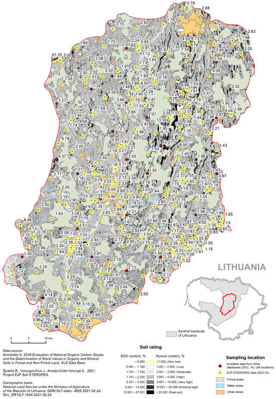
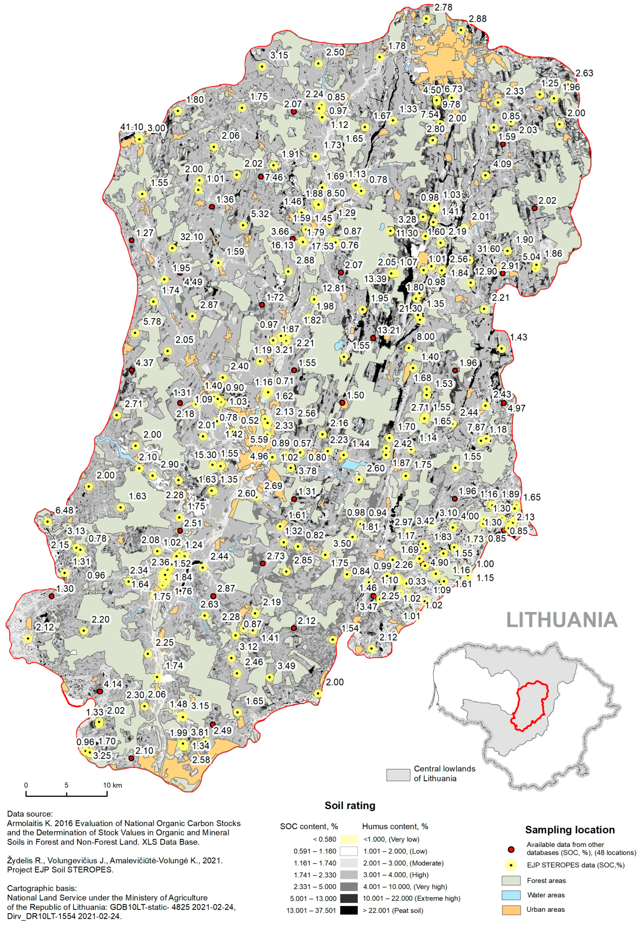
Figure 7.
SOC content in the topsoil (0–10 cm) of the Nevėžis Plain, according to the IGA third scenario (Created by second-level soil typological units (LTDK-99) contours of agricultural areas) [35].
Histic and mollic Gleysols (organomineral soils), which are characterized by moisture regimes SH(Ghi) and SH(Gfo), and Histosols (organic soils), which are characterized by the H moisture regime type, strongly stand out from the overall context of SOC accumulations (Figure 6b). These soils develop as hydromorphic soils, so the amount of SOC accumulated in them is strongly different from that of mineral soils (those reviewed above, Figure 6a). Therefore, in essence, the problem of identifying typical SOC values suitable for mapping lies only in mineral soils. The fundamental problem of this is the agrogenic transformation (cultivation, melioration) of these soils, which is a factor leveling the differences between them.
Based on the above-discussed results and stated assumptions, the map is drawn according to scenario III (Table 5). In the agricultural areas of the Nevėžio plain, soils with a high (1.741–2.330%) SOC content prevail (63.20%), and soils with a high and very high (1.741–5.000%) SOC content make up 79.09% of all soils used for agricultural purposes. According to the categories of humus content, these soils are classified as humus soils. Problem soils are those with a humus content of less than 2.0% or less than 1.16% organic carbon. There are only 1.13% of such soils in the agricultural areas of the Nevėžis Plain. This is associated with a small area of erosion, which is formed due to relief in the valley or on the slopes of a gully. These areas are expanding more and more due to the increasing intensity of agricultural activities and the expansion of their areas.
The total high humus content (as well as the amount of soil organic carbon) of the soils of the studied area is determined by natural conditions. Approximately 95% of all agricultural areas are covered by waterlogged soils, which are characterized by varying degrees of gley or gleyic properties (from SH(g4) to H). The performed analysis showed that the average amount of soil organic carbon in automorphic (AU) and semi-hydromorphic (SH (g4)–SH (Ghi)) soils is statistically significantly different, and the lack of organic carbon in the soil in areas of normal moisture soils is related with eroded soils. The most intensively used and largest agricultural areas are in gleyic soils (with moisture regime SH(g4)-SH(g8)) and gley soils (with moisture regime SH (G)).
4. Discussion
One of the most important indicators of soil quality is the amount of soil organic carbon, so much attention is paid to its mapping. Creating a detailed and objective map is a complicated task since the soil cover is complex and its structure is determined not only by natural but also by anthropogenic factors, which requires a large amount of data. The spatial differentiation of the amount of SOC depends not only on the continuous (most natural factors: mineral base, relief, moisture, vegetation cover) changing natural environment but also on discrete natural (soil material and the related layout of wetlands) and human economic activity measures and as a result emerging land use structure. The various interpolation methods used to solve this problem (e.g., inverse distance weighted (IDW), kriging, LPI, RBF, EBK technique) (Figure 3) do not give a sufficiently accurate result because these methods cannot estimate the spatial unevenness (discretion) factor of the soil cover properties of the mapped area and the structure of land features (non-mapped land: forests, lakes, water reservoirs, built-up areas, etc.). A study conducted in Turkey [36] also found that land use change has a major impact on SOC distribution. However, it was also emphasized that various interpolation methods (block kriging, co-kriging, IDW) used in SOC mapping do not fully reveal this, and the results are highly dependent on the quality of the data sampling design and size.
Since the soil cover is formed by natural zonal pedogenetic processes that lead to dominant mean SOC values and are transformed by azonal processes (both natural and anthropogenic) that cause significant fluctuations in SOC values, the direct application of interpolation methods has both advantages and disadvantages.
The best results with IDW are obtained when a dense sample is formed, taking into account the local characteristics of soil cover. Optimal outcomes are achieved when the sampling is directly linked to soil contours and their configuration. This aligns with the theoretical concept of this method. If the number of input points is sparse or heterogeneous, the results may not accurately represent the desired surface, leading to an underestimation of localized extremes in SOC variation [32].
LPI is most effective when the samples are taken on a grid, and the data values within the search neighborhood are normally distributed, as per [33].
Therefore, as can be seen from the results of the study, compared to the IDW method, the local extreme values of the SOC are even more smoothed.
The RBF method produces good results for gently varying soil surfaces such as elevation. However, the techniques are inappropriate when large changes in the surface values occur within short distances. This method is ideal for interpolating soil cover properties in lowland agricultural areas but not when the area includes zones with extreme SOC values—high or low—formed by azonal soil-forming processes, such as peat soils or eroded soils.
The EBK method, which combines kriging with regression analysis, offers predictions that are more accurate than regression or kriging alone [33]. It effectively integrates average and extreme values, leading to a relative increase in the occurrence of extreme SOC values in the area (Figure 8). This method also provides standard errors that are more accurate than other kriging methods and allows for precise prediction of moderately fluctuating data.
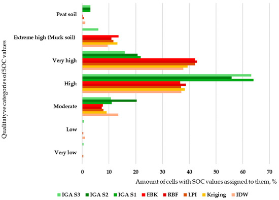
Figure 8.
Comparison of the application of different SOC mapping methods.
Figure 8 illustrates the distribution of statistical cells (10 × 10 m) (in percent) in the analyzed territory. The comparative analysis of the results (Figure 8) shows that standard interpolation methods are not suitable for SOC mapping on a regional scale when the territory is characterized by different relief, texture, and moisture conditions. Although this was not analyzed during the research, we would think that the application of different point arrangement principles (regular and irregular) in mapping would also have a significant impact on the results.
The soil cover is not a continuous object in terms of its properties (including SOC). It is characterized by different dominant (average) SOC values in individual geomorphological regions. Also, depending on the peculiarities of the relief, extreme values (eroded and/or waterlogged surfaces) can be characteristic. SOC mapping needs to reflect all of this. When evaluating the suitability of the methods, the following conditions of the territory were considered: eroded soils—1.65%, peat soils—3.04%, dominant soil—Gleyic Cambisol (CM-gl) (average SOC—2.15%)—42.27%, dominant soil moisture conditions—SH(g4-8) (average SOC–1, 9–2.0%). Of the IGA scenarios, the third scenario met all the criteria (especially soil erosion) and was therefore assessed.
The main weakness of interpolation methods in the context of our research is neighboring data averaging to interpolate uncertain values. As a result, the “leveling” of the analyzed area and the elimination of extreme SOC values will take place. From this perspective, the map generated by the IDW method retained the most extreme values. Nevertheless, the percentage of cells falling into the <0.580 and >13.001 ranges remained very low. However, when using kriging or EBK methods in mapping, the values of these intervals completely disappeared, or their percentage was close to zero.
Another important problem is that although soils with a high SOC content (1.741–2.330) predominate in the studied area, two SOC groups (high (1.741–2.330) and very high (2.331–5.000)) were dominant in the maps that were compiled using the interpolation method. The area of cells of the dominant group (high) decreased strongly, while the area of cells of the non-dominant (very high, about 15%) group more than doubled. The SOC group associated with very local areas (extremely high) also increased strongly, although the SOC values of this group are attributed to very local areas such as Mollic Gleysols (GL-mo) and Sapric Gleysols (GL-sa). They are characterized by a very localized, point-like spread. This shows that interpolation methods, in addition to the existing samples, without an additional specific layer of contours of “extemal” soils, cannot reliably model SOC distribution.
5. Conclusions
The formed and analyzed sample of 313 research points allowed us to calculate the average SOC concentration values of different soil typological units using different approaches. Most of these values are statistically significantly different from each other, so they can be considered representative of the soil cover of the moraine loam area of the Nevėžis Plain.
It is appropriate to structure the SOC data set according to two main factors: moisture regime and erosion, as these are the main factors determining the regularities of SOC differentiation in terrane surfaces. The application of this principle is relevant in order the SOC content in agricultural soils objectively to mapping.
The results show that the structuring of the SOC data set by soil classification units is appropriate only if soil moisture and erosion factors are coded in the indices of soil typological units.
The application of interpolation methods in SOC mapping can only be applied at a local scale, for example, in the territory, which is homogeneous in terms of soil forming factors, farming, and land use. The application of the interpolation methods (e.g., IDW, kriging) in the territory, which is characterized by the diversity of the conditions of soil formation, relief, and land use, is debatable because the localization and boundary discreteness of organic and organomineral soils (histosols, gleysols), soil erosion area, and forests are not evaluated. Therefore, the resulting image may be misleading.
The proposed IGA method is complex and knowledge-intensive, but its application can help create a geographically and pedologically-based SOC map and be adaptable to geographic conditions.
The results of the study suggest a recommendation that would increase the practical feasibility of the IGA approach and the research. In order to apply the IGA approach in SOC modeling, the following principles should be followed: the formation of objective, differential-density spatial statistical samples for data collection; the formation of samples according to soil moisture regime, degree of erosion, and land use; the development of contouring principles and a criteria algorithm that allows correct spatial interpolation of mean SOC values.
Supplementary Materials
The following supporting information can be downloaded at: https://www.mdpi.com/article/10.3390/su16125157/s1, Table S1: Basic statistics for 313 samples with determined SOC concentrations (%) under different soil types and moisture regimes.
Author Contributions
Conceptualization, J.V. and R.Ž.; methodology, J.V. and R.Ž.; software, J.V. and K.A.-V.; validation, J.V., R.Ž., and K.A.-V.; statistical analysis, K.A.-V.; GIS analysis, J.V.; investigation, J.V. and R.Ž.; data curation, J.V., R.Ž., and K.A.-V.; writing—original draft preparation, J.V.; writing—review and editing, J.V.; R.Ž., and K.A.-V.; visualization, J.V. and K.A.-V.; project administration, R.Ž.; All authors have read and agreed to the published version of the manuscript.
Funding
This work was supported by the European Union’s Horizon H2020 research and innovation European Joint Program Cofound on Agricultural Soil Management (EJP-SOIL grant number 862695) and was carried out in the framework of the STEROPES of EJP-SOIL.
Institutional Review Board Statement
Not applicable.
Informed Consent Statement
Not applicable.
Data Availability Statement
Data is contained within the article and Supplementary Materials.
Conflicts of Interest
The authors declare no conflicts of interest.
References
- Wei, J.B.; Xiao, D.N.; Zeng, H.; Fu, Y.K. Spatial variability of soil properties in relation to land use and topography in a typical small watershed of the black soil region, northeastern China. Environ. Geol. 2008, 53, 1663–1672. [Google Scholar] [CrossRef]
- Bhunia, G.S.; Shit, P.K.; Maiti, R. Comparison of GIS-based interpolation methods for spatial distribution of soil organic carbon (SOC). J. Saudi Soc. Agric. Sci. 2018, 17, 114–126. [Google Scholar] [CrossRef]
- Galvydytė, D. Geografų indėlis į Lietuvos dirvožemio mokslą. Geogr. Metrašt. 2009, 42, 114–140. (In Lithuanian) [Google Scholar]
- Buivydaitė, V.V.; Vaičys, M.; Juodis, J.; Motuzas, A. Lithuanian Soil Classification; Lietuvos Mokslas Book: Vilnius, Lithuania, 2001; Volume 34, p. 137. (In Lithuanian) [Google Scholar]
- IUSS Working Group WRB. International Soil Classification System for Naming Soils and Creating Legends for Soil Maps. In World Reference Base for Soil Resources, 4th ed.; International Union of Soil Sciences (IUSS): Vienna, Austria, 2022. [Google Scholar]
- Dirv_DR10LT. Spatial Data Set of Soil of the Territory of the Republic of Lithuania at Scale 1:10,000. 2022. Available online: https://www.geoportal.lt/metadata-catalog/catalog/search/resource/details.page?uuid=%7B449450A9-AD8C-6E9E-6FCB-06A0584BF88C%7D (accessed on 6 March 2023).
- DirvAgroch_DR10LT. Spatial Data Set of Soil Organic Carbon of the Territory of the Republic of Lithuania at Scale 1:10,000. 2023. Available online: https://www.geoportal.lt/metadata-catalog/catalog/search/resource/details.page?uuid=%7BF14575DC-DE8B-4BD6-B52B-E164EA526534%7D (accessed on 30 June 2023).
- Armolaitis, K.; Varnagirytė-Kabašinskienė, I.; Žemaitis, P.; Stakėnas, V.; Beniušis, R.; Kulbokas, G.; Urbaitis, G. Evaluation of organic carbon stocks in mineral and organic soils in Lithuania. Soil Use Manag. 2021, 38, 355–368. [Google Scholar] [CrossRef]
- Li, T.; Xia, A.; McLaren, T.I.; Pandey, R.; Xu, Z.; Liu, H.; Manning, S.; Madgett, O.; Duncan, S.; Rasmussen, P.; et al. Preliminary Results in Innovative Solutions for Soil Carbon Estimation: Integrating Remote Sensing, Machine Learning, and Proximal Sensing Spectroscopy. Remote Sens. 2023, 15, 5571. [Google Scholar] [CrossRef]
- Wu, T.; Wu, Q.; Zhuang, Q.; Li, Y.; Yao, Y.; Zhang, L.; Xing, S. Optimal Sample Size for SOC Content Prediction for Mapping Using the Random Forest in Cropland in Northern Jiangsu, China. Eurasian Soil Sci. 2022, 55, 1689–1699. [Google Scholar] [CrossRef]
- Negassa, M.K.; Haile, M.; Feyisa, G.L.; Wogi, L.; Merga, F. Modeling and mapping spatial distribution of baseline soil organic carbon stock, a case of West Hararghe, Oromia Regional State, Eastern Ethiopia. Geol. Ecol. Landsc. 2023, 1–16. [Google Scholar] [CrossRef]
- Adhikari, K.; Hartemink, A.E.; Minasny, B.; Bou Kheir, R.; Greve, M.B.; Greve, M.H. Digital Mapping of Soil Organic Carbon Contents and Stocks in Denmark. PLoS ONE 2014, 9, e105519. [Google Scholar] [CrossRef] [PubMed]
- Li, T.; Cui, L.; Xu, Z.; Hu, R.; Joshi, P.K.; Song, X.; Tang, L.; Xia, A.; Wang, Y.; Guo, D.; et al. Quantitative Analysis of the Research Trends and Areas in Grassland Remote Sensing: A Scientometrics Analysis of Web of Science from 1980 to 2020. Remote Sens. 2021, 13, 1279. [Google Scholar] [CrossRef]
- Marchetti, A.; Piccini, C.; Francaviglia, R.; Mabit, L. Spatial distribution of soil organic matter using geostatistics: A key indicator to assess soil degradation status in Central Italy. Pedosphere 2012, 22, 230–242. [Google Scholar] [CrossRef]
- Castaldi, F.; Koparan, M.H.; Wetterlind, J.; Žydelis, R.; Vinci, I.; Savas, A.O.; Kıvrak, C.; Tunçay, T.; Volungevičius, J.; Obber, S.; et al. Assessing the capability of Sentinel-2 time-series to estimate soil organic carbon and clay content at local scale in croplands. ISPRS J. Photogramm. Remote Sens. 2023, 199, 40–60. [Google Scholar] [CrossRef]
- Steffensen, J.F. Interpolation, 2nd ed.; Dover: Mineola, NY, USA, 2006. [Google Scholar]
- Schulp, C.J.E.; Verbung, P.H. Effect of land use history and site factors on spatial variation of soil organic carbon across a physiographic region. Agric. Ecosyst. Environ. 2009, 133, 86–97. [Google Scholar] [CrossRef]
- Fan, M.; Lal, R.; Zhang, H.; Marganot, A.J.; Wu, J.; Wu, P.; Zhang, L.; Yao, J.; Chen, F.; Gao, C. Variability, and determinants of soil organic matter under different land uses and soil types in eastern China. Soil Tillage Res. 2020, 198, 104544. [Google Scholar] [CrossRef]
- Haynes, R.J.; Naidu, R. Influence of lime, fertilizer and manure applications on soil organic matter content and soil physical conditions: A review. Nutr. Cycl. Agroecosyst. 1998, 51, 123–137. [Google Scholar] [CrossRef]
- Szostek, M.; Szpunar-Krok, E.; Pawlak, R.; Stanek-Tarkowska, J.; Ilek, A. Effect of Different Tillage Systems on Soil Organic Carbon and Enzymatic Activity. Agronomy 2022, 12, 208. [Google Scholar] [CrossRef]
- Bardule, A.; Lupikis, A.; Butlers, A.; Lazdins, A. Organic carbon stock in different types of mineral soils in cropland and grassland in Latvia. Zemdirb.-Agric. 2017, 104, 3–8. [Google Scholar] [CrossRef]
- Kõlli, R.; Ellermae, O.; Koster, T.; Lemetti, I.; Asi, E.; Kauer, K. Stocks of organic carbon in Estonian soils. Est. J. Earth Sci. 2009, 58, 95–108. [Google Scholar] [CrossRef]
- Metzger, M.J.; Shkaruba, A.D.; Jongman, R.H.G.; Bunce, R.G.H. Description of the European Environmental Zones and Strata; Alterra Report: Wageniningen, The Netherland, 2012; p. 154. [Google Scholar]
- Metzger, M.J.; Bunce, R.G.H.; Jongman, R.H.G.; Mücher, C.A.; Watkins, J.W. A climatic stratification of the environment of Europe. Glob. Ecol. Biogeogr. 2005, 14, 549–563. [Google Scholar] [CrossRef]
- Bukantis, A. Agroklimatinis rajonavimas. Liet. Nac. Atlasas 2014, 1T, 74. (In Lithuanian) [Google Scholar]
- Rinterknecht, V.R.; Bitinas, A.; Clark, P.U.; Raisbeck, G.M.; Yiou, F.; Brook, E.J. Timing of the last deglaciation in Lithuania. Boreas 2008, 37, 426–433. [Google Scholar] [CrossRef]
- Tylmann, K.; Uscinowicz, S. Timing of the last deglaciation phases in the southern Baltic area inferred from Bayesian age modeling. Quat. Sci. Rev. 2022, 287, 107563. [Google Scholar] [CrossRef]
- Guobytė, R.; Kavaliauskas, P. Geomorfologinis rajonavimas. LLiet. Nac. Atlasas 2014, 1T, 52. (In Lithuanian) [Google Scholar]
- NMA-Paseliai (National Paying Agency—Crops) Spatial Crop Declaration Data Set of the Territory of the Republic of Lithuania at Scale 1:10,000. 2023. Available online: https://www.geoportal.lt/metadata-catalog/catalog/search/resource/details.page?uuid=%7B7AF3F5B2-DC58-4EC5-916C-813E994B2DCF%7D (accessed on 13 October 2023).
- Nikitin, B.A. Methods for soil humus determination. Agric. Chem. 1999, 3, 156–158. [Google Scholar]
- Armolaitis, K.; Stakėnas, V.; Varnagirytė-Kabašinskienė, I.; Žemaitis, P.; Araminienė, V.; Buivydaitė, V.V.; Muraškienė, M.; Armolaitis, T. Evaluation of National Organic Carbon Stocks and the Determination of Stock Values in Organic and Mineral Soils in Forest and Non-Forest Land; Report; Ministry of Environment of the Republic of Lithuania: Kaunas-Girionys, Lithuania, 2016; p. 90. (In Lithuanian)
- Watson, D.F.; Philip, G.M. A Refinement of Inverse Distance Weighted Interpolation. Geoprocessing 1985, 2, 315–327. [Google Scholar]
- ArcGIS Pro Documentation. ESRI. Available online: https://pro.arcgis.com/en/pro-app/latest/tool-reference/spatial-analyst/understanding-interpolation-analysis.htm (accessed on 16 May 2024).
- GDB10LT-Static. Spatial Data Set of Georeferenced Base Map of the Territory of the Republic of Lithuania at Scale 1:10,000. 2023. Available online: https://www.geoportal.lt/metadata-catalog/catalog/search/resource/details.page?uuid=%7B3FCEEFFD-9704-4A0C-96F3-4CF5DBA94F15%7D (accessed on 25 January 2023).
- Armolaitis, K. Evaluation of National Organic Carbon Stocks and the Determination of Stock Values in Organic and Mineral Soils in Forest and Non-Forest Land. XLS Data Base 2016.
- Göl, C.; Bulut, S.; Bolat, F. Comparison of different interpolation methods for spatial distribution of soil organic carbon and some soil properties in the Black Sea backward region of Turkey. J. Afr. Earth Sci. 2017, 134, 85–91. [Google Scholar] [CrossRef]


Disclaimer/Publisher’s Note: The statements, opinions and data contained in all publications are solely those of the individual author(s) and contributor(s) and not of MDPI and/or the editor(s). MDPI and/or the editor(s) disclaim responsibility for any injury to people or property resulting from any ideas, methods, instructions or products referred to in the content. |
© 2024 by the authors. Licensee MDPI, Basel, Switzerland. This article is an open access article distributed under the terms and conditions of the Creative Commons Attribution (CC BY) license (https://creativecommons.org/licenses/by/4.0/).