


Sinkhole Risk-Based Sensor Placement for Leakage Localization in Water Distribution Networks with a Data-Driven Approach


Abstract
1. Introduction
2. Materials and Methods
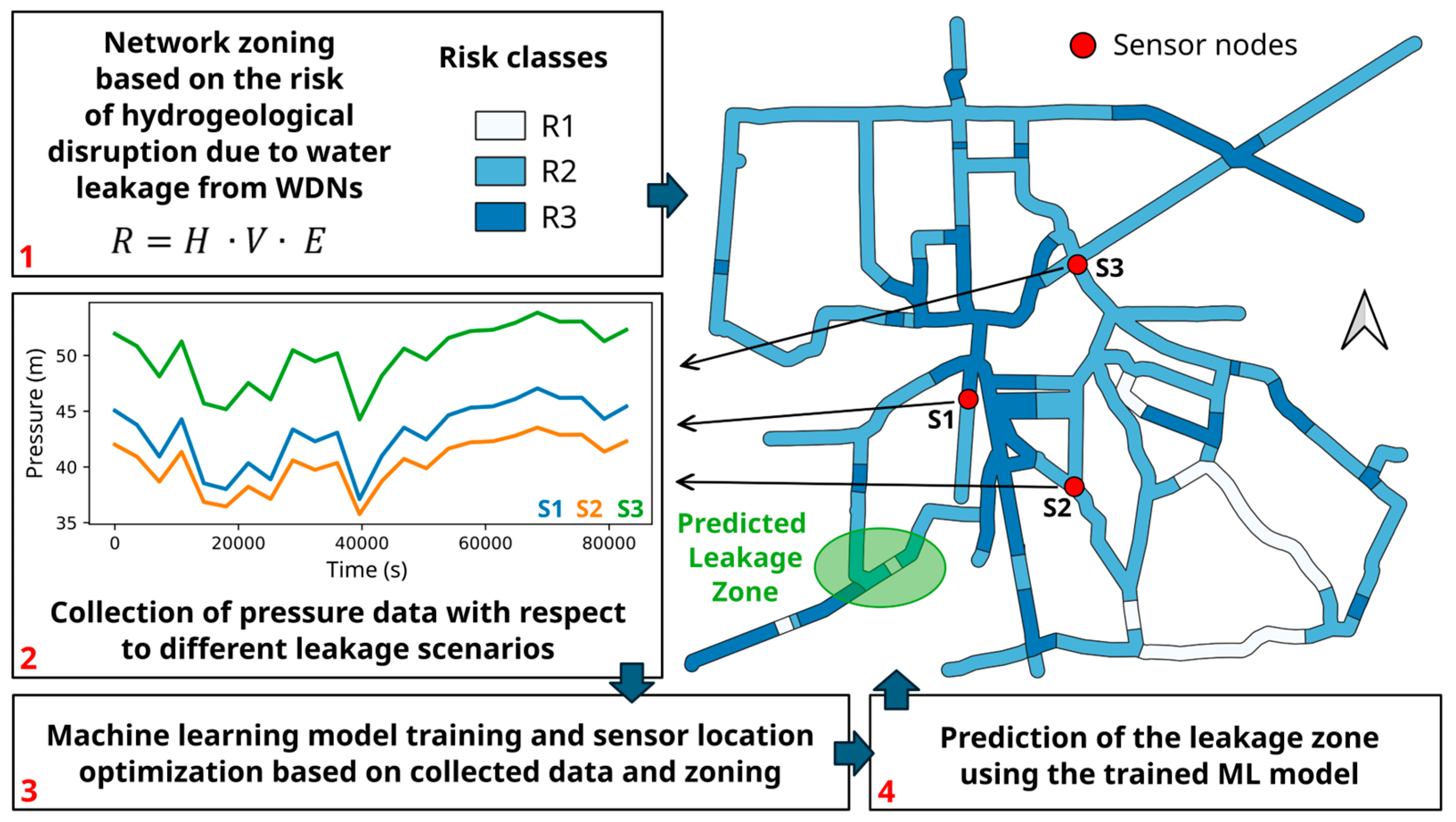
- WDN zoning based on the risk from Hydrogeological Disruption due to Leakage (HDL) (Figure 1, step 1);
- Use of a hydraulic simulator to generate WDN pressure data under different demand conditions and different leakage scenarios (Figure 1, step 2);
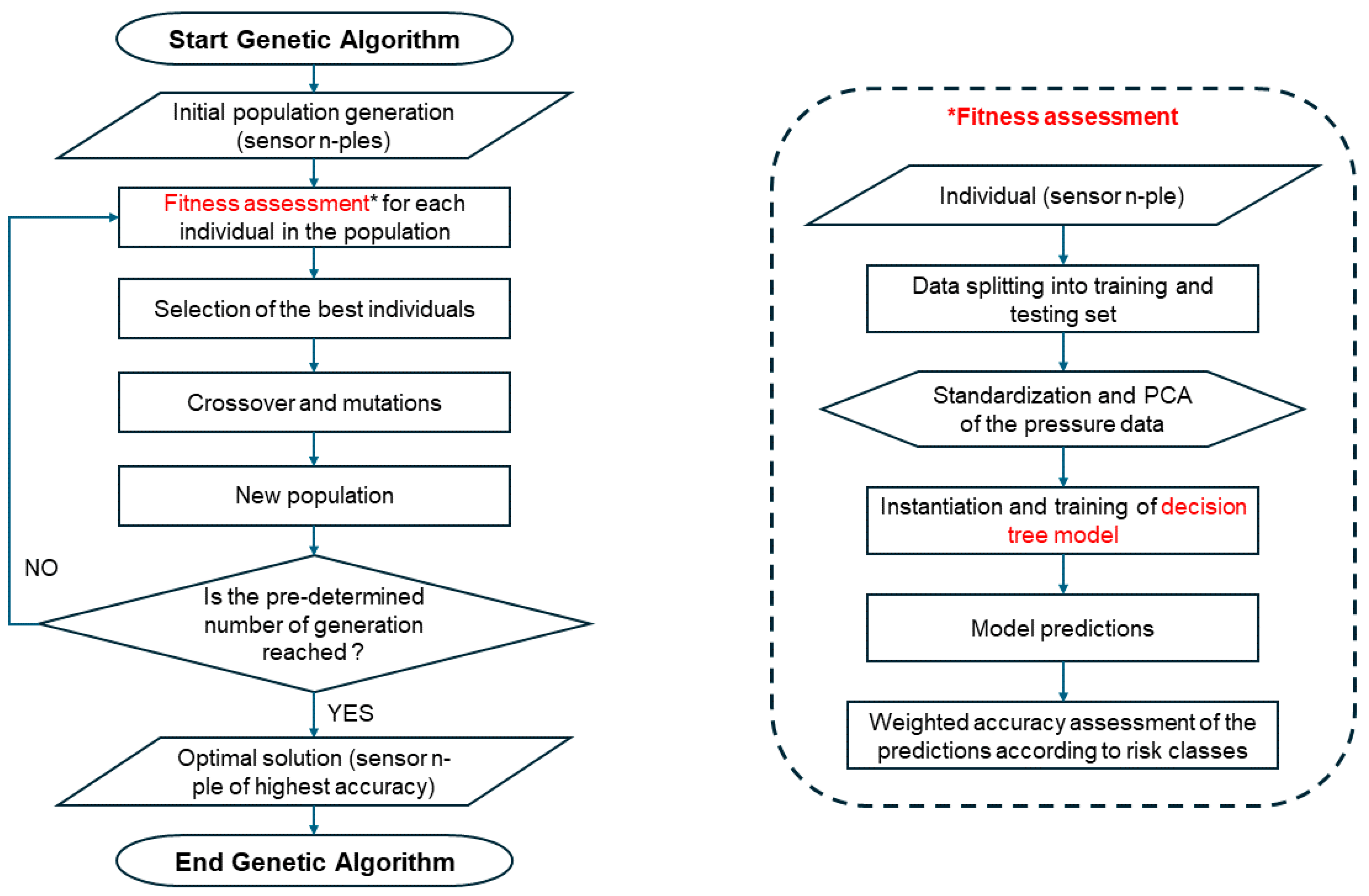
- Use of a GA for the approximate solution of the OSP problem, aiming at maximizing the likelihood of detecting leakages in areas at higher risk from HDL (Figure 1, step 3);
- During the GA application, use of an ML model to train and evaluate the sets of sensors, i.e., the candidate solutions of the OSP problem (Figure 1, steps 3–4).
2.1. Risk Evaluation of Hydrogeological Disruption Due to Water Leaks
- -
- the hazard H: the likelihood of occurrence of the dangerous event, i.e., the hydrogeological disruption caused by a non-detected leak with a given magnitude at a given location, ranging from 0 (null likelihood) to 1 (maximum likelihood);
- -
- the vulnerability V: the expected degree of damage due to the impact of the hazardous event (hydrogeological disruption due to leakage) on the system (soil, urban infrastructures and human elements), ranging from 0 (no damage) to 1 (total disruption) [39];
- -
- the exposure E: the socio-economic importance of goods, structures, and infrastructures, as well as the presence of people in the at-risk area.
2.2. Pressure Data
- -
- leakages are considered at junction nodes only;
- -
- each scenario is characterized by a single leaking node;
- -
- the total number of leakage scenarios is equal to the number NN of junction nodes;
- -
- each leakage scenario is evaluated over a simulation time of T = 50 days.
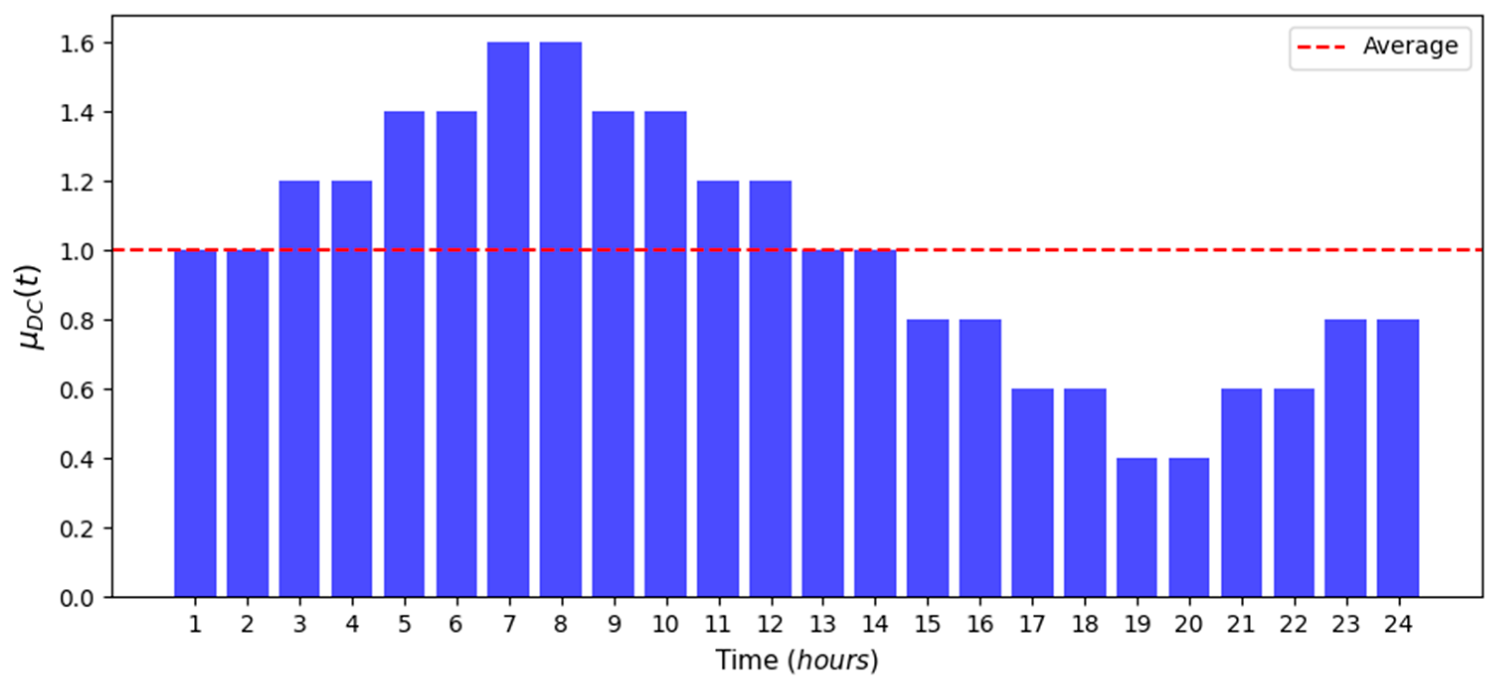
2.2.1. Demand Modelling
2.2.2. Water Leakage Modelling
2.3. Pressure Sensor Training and Optimal Positioning
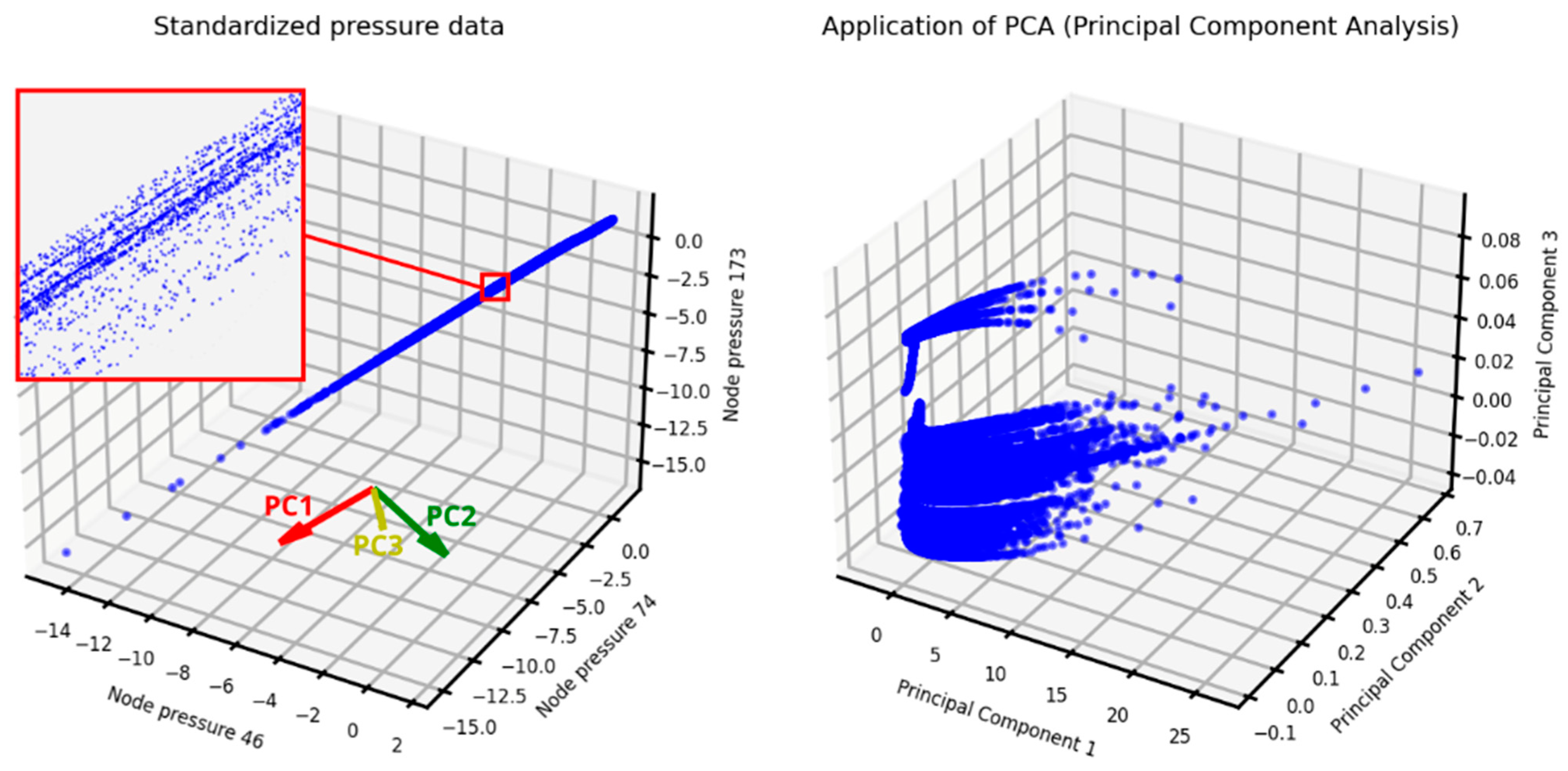
2.3.1. Data Pre-Processing
2.3.2. Decision Tree Classifier
2.3.3. Sensor Position Optimization
3. Results and Discussion
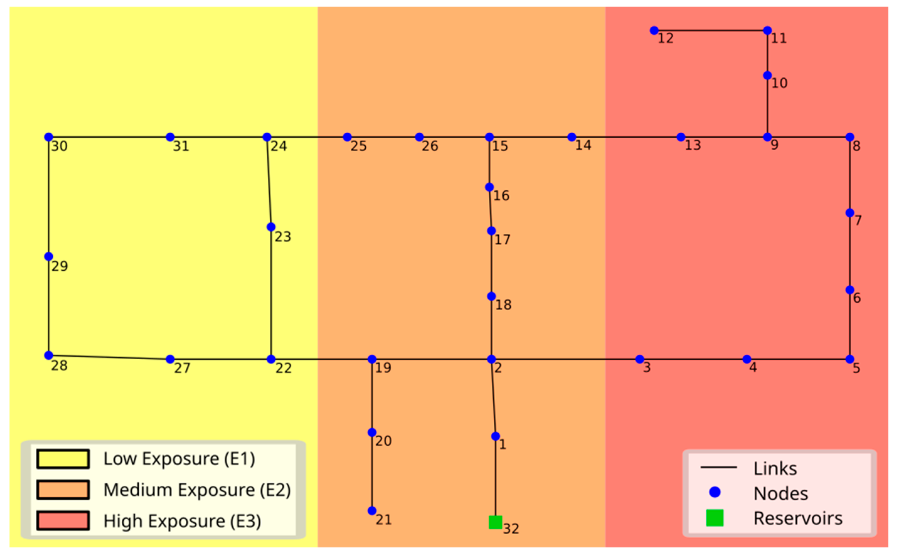
3.1. Hanoi Network
- -
- 32 junction nodes;
- -
- 34 pipes (links);
- -
- 1 inlet point (reservoir);
- -
- pipe diameters from 304.8 to 1016 mm.
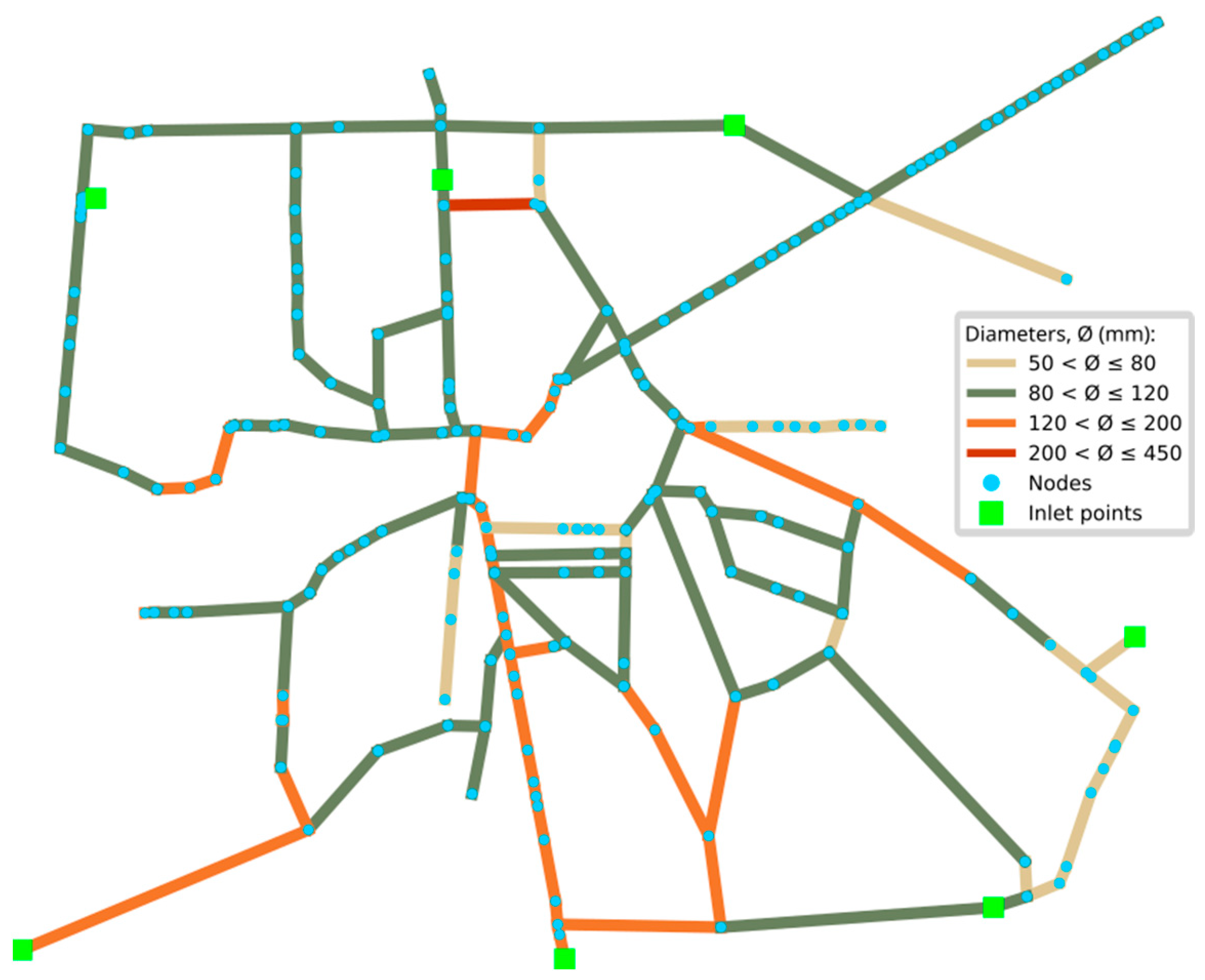
3.2. Real Network 1
- -
- 206 junctions;
- -
- 231 links;
- -
- 7 inlet points with almost constant piezometric head;
- -
- pipe diameters from 53.6 to 406.4 mm.
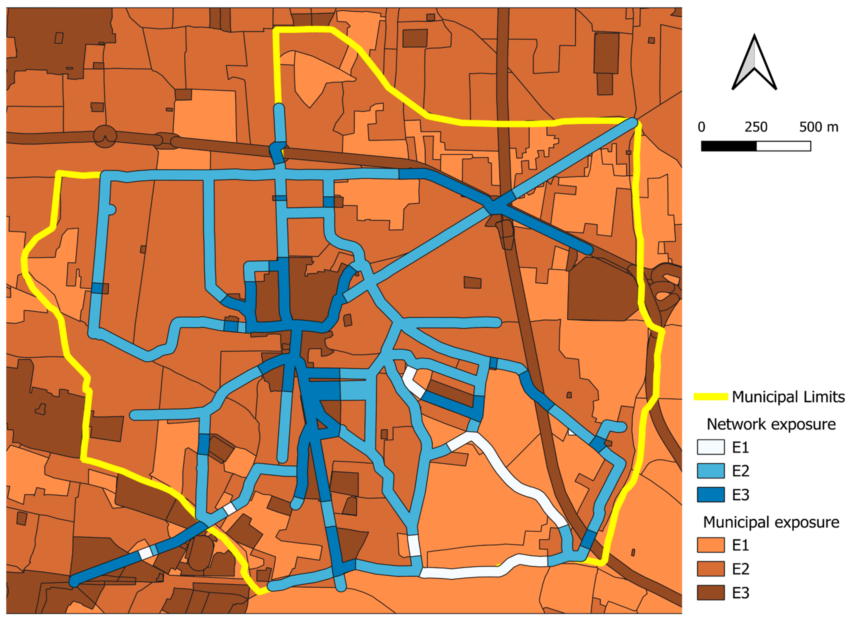
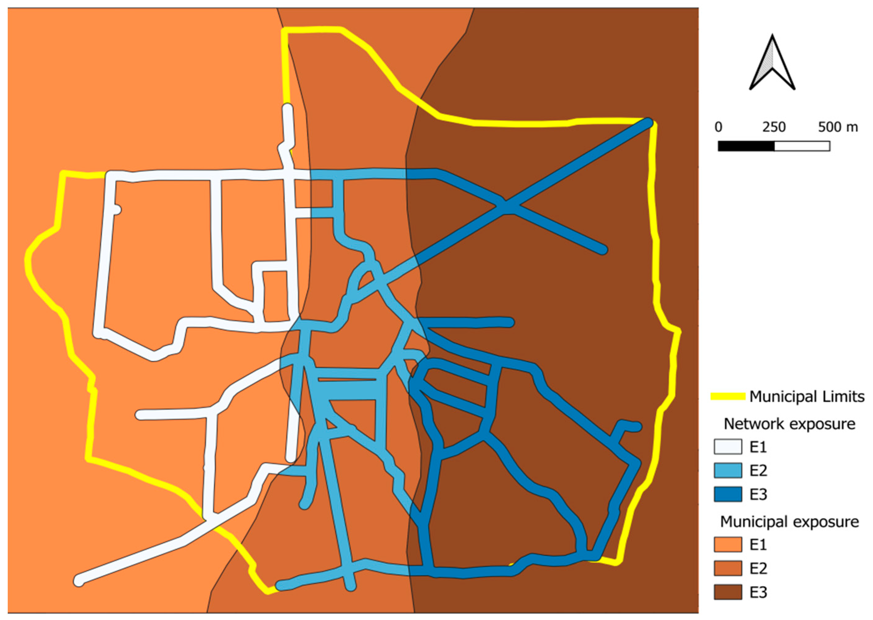
3.2.1. Risk Zoning Based on Exposure to HDL
- (1)
- The census information (available at https://www.istat.it/, accessed on 15 January 2024) is used to evaluate the distribution of the population density through the municipality.
- (2)
- Information levels on structures and infrastructure at the municipality scale are collected (from https://www.istat.it/, accessed on 15 January 2024).
- (3)
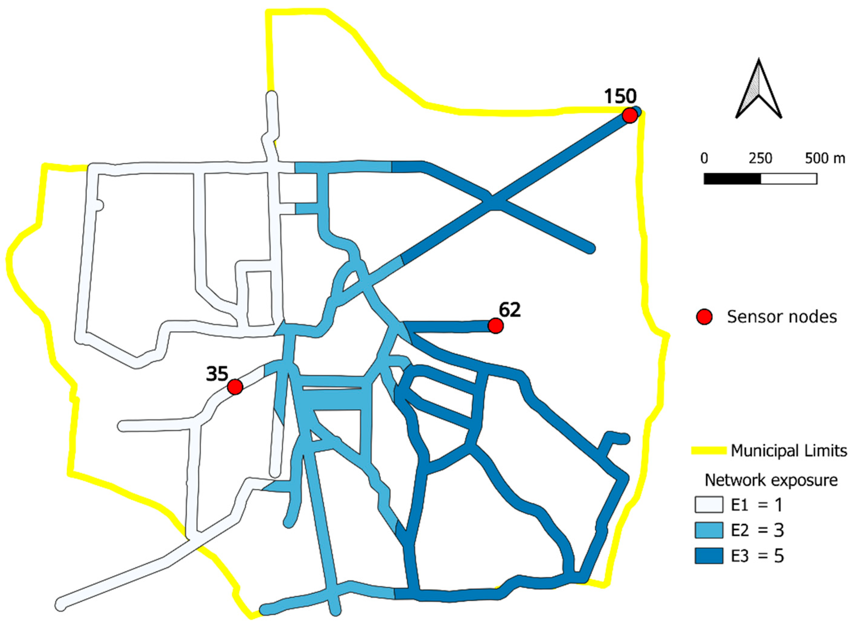
- Three municipality exposure classes are introduced as follows (see the brown areas in Figure 8):
- (a)
- class E1 groups areas with low population density, where strategic infrastructures are absent, and areas with agricultural land uses;
- (b)
- class E2 represents areas with medium population density and buildings, mostly residential, with modest public or strategic functions;
- (c)
- class E3 applies to areas with significant population density, or areas with infrastructure, industries and buildings that have important public or strategic functions.
- (4)
- A buffer area whose width is W = 25 m is constructed along the WDN pipe. The buffer area individuates the municipality elements that can be potentially impacted by HDL because they are adjacent to the WDN pipes. The exposure class of the municipality elements is attributed also to homogeneous buffer sections (white and blue areas in Figure 8).
- (5)
- The exposure class of the buffer section is inherited by WDN junction nodes falling in it.
3.2.2. Fictious Risk Zoning
4. Conclusions
- -
- the proposed risk-based methodology that accounts for the adverse impact due to hydrogeological disruption from undetected leaks is advantageous over conventional non-risk-based methods (that treat all elements at risk equally), since it prioritizes monitoring locations where more people and critical infrastructure could be potentially affected in the event of a leak, increasing the likelihood of leakage localization in higher risk zones due to sinkhole formation;
- -
- the ability of the proposed methodology to detect generic leakage is not adversely affected, facilitating the additional goal of reducing water resource depletion.
Author Contributions
Funding
Data Availability Statement
Acknowledgments
Conflicts of Interest
Nomenclature
| CV | coefficient of variation |
| DC(t) | demand pattern coefficient at time t |
| DT | Decision Tree |
| E | Exposure |
| ECi | emitter coefficient of the i-th node |
| GA | Genetic Algorithm |
| GIS | Geographic information systems |
| H | Hazard |
| HDL | Hydrogeological Disruption due to Leakage |
| hi | piezometric head at the i-th node |
| hst,i | standardized value of hi |
| ISTAT | Italian National Institute of Statistics |
| Mk(P) | localization accuracy of the set of sensors P referred to the leakages from the cluster Ωk |
| ML | Machine Learning |
| Mp(P) | fitness of the set of senors P |
| NAk(P) | number of accurate predictions made by the set of sensors P regarding the leakages from the nodes of Ωk |
| NC | number of localization clusters |
| Nk | number of leakage scenarios from the nodes of Ωk |
| NN | number of junction nodes in the WDN |
| NR | number of risk levels |
| NS | number of pressure sensors |
| OSP | Optimal sensor placement |
| P | set of NS pressure sensors |
| PCA | Principal component analysis |
| Qi | flow rate through the emitter at the i-th node |
| qBi | base demand at the i-th node |
| qi(t) | demand at the i-th node at time t |
| R | Risk |
| T | simulation time |
| t | time |
| USD | United States dollar |
| W | buffer area width |
| WDN | water distribution network |
| V | Vulnerability |
| standard deviation of hi | |
| Ωk | Subset (localization cluster) of Ω |
| mean of hi | |
| µDC(t) | Average demand coefficient at time t |
| Subscripts | |
| i | Subscript for nodes |
| k | Subscript for the generic localization cluster |
Appendix A
References
- Gosling, S.N.; Arnell, N.W. A global assessment of the impact of climate change on water scarcity. Clim. Chang. 2016, 134, 371–385. [Google Scholar] [CrossRef]
- Fan, X.; Wang, X.; Zhang, X.; Yu, X. Machine learning based water pipe failure prediction: The effects of engineering, geology, climate and socio-economic factors. Reliab. Eng. Syst. Saf. 2022, 219, 108185. [Google Scholar] [CrossRef]
- Zaman, D.; Gupta, A.K.; Uddameri, V.; Tiwari, M.K.; Ghosal, P.S. Hydraulic performance benchmarking for effective management of water distribution networks: An innovative composite index-based approach. J. Environ. Manag. 2021, 299, 113603. [Google Scholar] [CrossRef] [PubMed]
- Robles-Velasco, A.; Cortés, P.; Muñuzuri, J.; De Baets, B. Prediction of pipe failures in water supply networks for longer time periods through multi-label classification. Expert. Syst. Appl. 2023, 213 Pt B, 119050. [Google Scholar] [CrossRef]
- Covelli, C.; Cozzolino, L.; Cimorelli, L.; Della Morte, R.; Pianese, D. Optimal location and setting of PRVs in WDS for leakage minimization. Water Resour. Manag. 2016, 30, 1803–1817. [Google Scholar] [CrossRef]
- Dastpak, P.; Sousa, R.L.; Dias, D. Soil Erosion Due to Defective Pipes: A Hidden Hazard Beneath Our Feet. Sustainability 2023, 15, 8931. [Google Scholar] [CrossRef]
- Alzarooni, E.; Ali, T.; Atabay, S.; Yilmaz, A.G.; Mortula, M.M.; Fattah, K.P.; Khan, Z. GIS-Based Identification of Locations in Water Distribution Networks Vulnerable to Leakage. Appl. Sci. 2023, 13, 4692. [Google Scholar] [CrossRef]
- Liemberger, R.; Wyatt, A. Quantifying the Global Non-Revenue Water Problem. Water Supply 2019, 19, 831–837. [Google Scholar] [CrossRef]
- ISTAT. Le Statistiche dell’ISTAT Sull’acqua—Anni 2020–2022. Report. 2023. Available online: https://www.istat.it/it/files//2023/03/GMA-21marzo2023.pdf (accessed on 19 April 2024). (In Italian).
- Karim, M.R.; Abbaszadegan, M.; LeChevallier, M. Potential for pathogen intrusion during pressure transients. J. Am. Water Work. 2003, 95, 134–146. [Google Scholar] [CrossRef]
- Ali, H.; Choi, J.-h. A Review of Underground Pipeline Leakage and Sinkhole Monitoring Methods Based on Wireless Sensor Networking. Sustainability 2019, 11, 4007. [Google Scholar] [CrossRef]
- Tharp, T.M. Mechanics of upward propagation of cover-collapse sinkholes. Eng. Geol. 1999, 52, 23–33. [Google Scholar] [CrossRef]
- Nisio, S.; Caramanna, G.; Ciotoli, G. Sinkholes in Italy: First results on the inventory and analysis. Geol. Soc. Lond. Spec. Publ. 2007, 279, 23–45. [Google Scholar] [CrossRef]
- Guo, S.; Shao, Y.; Zhang, T.; Zhu, D.Z.; Zhang, Y. Physical modeling on sand erosion around defective sewer pipes under the influence of groundwater. J. Hydraul. Eng. 2013, 139, 1247–1257. [Google Scholar] [CrossRef]
- Rodriguez-Espinosa, P.F.; Ochoa-Guerrero, K.M.; Milan-Valdes, S.; Teran-Cuevas, A.R.; Hernandez-Silva, M.G.; San Miguel-Gutierrez, J.C.; Caracheo-Gonzalez, J.J.; Creuheras Diaz, S. Impacts on groundwater-related anthropogenic activities on the development of sinkhole hazards: A case study from Central Mexico. Environ. Earth Sci. 2023, 82, 358. [Google Scholar] [CrossRef]
- Lee, E.J.; Shin, S.Y.; Ko, B.C.; Chang, C. Early sinkhole detection using a drone-based thermal camera and image processing. Infrared Phys. Technol. 2016, 78, 223–232. [Google Scholar] [CrossRef]
- Guarino, P.M.; Santo, A.; Forte, G.; De Falco, M.; Niceforo, D.M.A. Analysis of a database for anthropogenic sinkhole triggering and zonation in the Naples hinterland (Southern Italy). Nat. Hazards 2018, 91, 173–192. [Google Scholar] [CrossRef]
- Tufano, R.; Guerriero, L.; Annibali Corona, M.; Bausilio, G.; Di Martire, D.; Nisio, S.; Calcaterra, D. Anthropogenic sinkholes of the city of Naples, Italy: An update. Nat. Hazards 2022, 112, 2577–2608. [Google Scholar] [CrossRef]
- Sahu, P.; Lokhande, R.D. An Investigation of Sinkhole Subsidence and its Preventive Measures in Underground Coal Mining. Procedia Earth Planet. Sci. 2015, 11, 63–75. [Google Scholar] [CrossRef]
- Zou, Q.; Chen, Z.; Cheng, Z.; Liang, Y.; Xu, W.; Wen, P.; Zhang, B.; Liu, H.; Kong, F. Evaluation and intelligent deployment of coal and coalbed methane coupling coordinated exploitation based on Bayesian network and cuckoo search. Int. J. Min. Sci. Technol. 2022, 32, 1315–1328. [Google Scholar] [CrossRef]
- Zhang, D.-M.; Du, W.-W.; Peng, M.-Z.; Feng, S.-J.; Li, Z.-L. Experimental and numerical study of internal erosion around submerged defective pipe. Tunn. Undergr. Space Technol. 2020, 97, 103256. [Google Scholar] [CrossRef]
- Tan, Y.; Long, Y.Y. Review of cave-in failures of urban roadways in China: A database. J. Perform. Constr. Facil. 2021, 35, 04021080. [Google Scholar] [CrossRef]
- Indiketiya, S.; Jegatheesan, P.; Rajeev, P.; Kuwano, R. The influence of pipe embedment material on sinkhole formation due to erosion around defective sewers. Transp. Geotech. 2019, 19, 110–125. [Google Scholar] [CrossRef]
- Tan, F.; Tan, W.; Yan, F.; Qi, X.; Li, Q.; Hong, Z. Model Test Analysis of Subsurface Cavity and Ground Collapse Due to Broken Pipe Leakage. Appl. Sci. 2022, 12, 13017. [Google Scholar] [CrossRef]
- Guarino, P.M.; Nisio, S. Anthropogenic sinkholes in the territory of the city of Naples (Southern Italy). Phys. Chem. Earth Parts A/B/C 2012, 49, 92–102. [Google Scholar] [CrossRef]
- Kim, K.; Kim, J.; Kwak, T.Y.; Chung, C.K. Logistic regression model for sinkhole susceptibility due to damaged sewer pipes. Nat. Hazards 2018, 93, 765–785. [Google Scholar] [CrossRef]
- Casillas, M.; Puig, V.; Garza-Castañón, L.; Rosich, A. Optimal Sensor Placement for Leak Location in Water Distribution Networks Using Genetic Algorithms. Sensors 2013, 13, 14984–14985. [Google Scholar] [CrossRef]
- Steffelbauer, D.B.; Fuchs-Hanusch, D. Efficient Sensor Placement for Leak Localization Considering Uncertainties. Water Resour. Manag. 2016, 30, 5517–5533. [Google Scholar] [CrossRef]
- Cugueró-Escofet, M.À.; Puig, V.; Quevedo, J. Optimal Pressure Sensor Placement and Assessment for Leak Location Using a Relaxed Isolation Index: Application to the Barcelona Water Network. Control Eng. Pract. 2017, 63, 1–12. [Google Scholar] [CrossRef]
- Forconi, E.; Kapelan, Z.; Ferrante, M.; Mahmoud, H.; Capponi, C. Risk-based sensor placement methods for burst/leak detection in water distribution systems. Water Supply 2017, 17, 1663–1672. [Google Scholar] [CrossRef]
- Li, J.; Wang, C.; Qian, Z.; Lu, C. Optimal Sensor Placement for Leak Localization in Water Distribution Networks Based on a Novel Semi-Supervised Strategy. J. Process Control 2019, 82, 13–21. [Google Scholar] [CrossRef]
- Hu, Z.; Chen, W.; Chen, B.; Tan, D.; Zhang, Y.; Shen, D. Robust Hierarchical Sensor Optimization Placement Method for Leak Detection in Water Distribution System. Water Resour. Manag. 2021, 35, 3995–4008. [Google Scholar] [CrossRef]
- Hu, Z.; Chen, W.; Tan, D.; Chen, B.; Shen, D. Multi-Objective and Risk-Based Optimal Sensor Placement for Leak Detection in a Water Distribution System. Environ. Technol. Innov. 2022, 28, 102565. [Google Scholar] [CrossRef]
- Cheng, M.; Li, J. Optimal Sensor Placement for Leak Location in Water Distribution Networks: A Feature Selection Method Combined with Graph Signal Processing. Water Res. 2023, 242, 120313. [Google Scholar] [CrossRef] [PubMed]
- Zeng, X.; Yu, Y.; Yang, S.; Lv, Y.; Sarker, M.N.I. Urban Resilience for Urban Sustainability: Concepts, Dimensions, and Perspectives. Sustainability 2022, 14, 2481. [Google Scholar] [CrossRef]
- United Nations. General Assembly Resolution A/RES/70/1. In Transforming Our World, the 2030 Agenda for Sustainable Development; United Nations: New York, NY, USA, 2015; Available online: https://sdgs.un.org/2030agenda (accessed on 15 January 2024).
- Gao, Y.; Alexander, E.C. Sinkhole hazard assessment in Minnesota using a decision tree model. Environ. Geol. 2008, 54, 945–956. [Google Scholar] [CrossRef]
- Taheri, K.; Shahabi, H.; Chapi, K.; Shirzadi, A.; Gutiérrez, F.; Khosravi, K. Sinkhole susceptibility mapping: A comparison between Bayes-based machine learning algorithms. Land. Degrad. Dev. 2019, 30, 730–745. [Google Scholar] [CrossRef]
- Bianchini, S.; Confuorto, P.; Intrieri, E.; Sbarra, P.; Di Martire, D.; Calcaterra, D.; Fanti, R. Machine learning for sinkhole risk mapping in Guidonia-Bagni di Tivoli plain (Rome), Italy. Geocarto Int. 2024, 37, 16687–16715. [Google Scholar] [CrossRef]
- Ali, H.; Choi, J.-h. Risk Prediction of Sinkhole Occurrence for Different Subsurface Soil Profiles due to Leakage from Underground Sewer and Water Pipelines. Sustainability 2020, 12, 310. [Google Scholar] [CrossRef]
- Karoui, T.; Jeong, S.-Y.; Jeong, Y.-H.; Kim, D.-S. Experimental Study of Ground Subsidence Mechanism Caused by Sewer Pipe Cracks. Appl. Sci. 2018, 8, 679. [Google Scholar] [CrossRef]
- Crichton, D. The Risk Triangle. In Natural Disaster Management; Ingleton, J., Ed.; Tudor Rose: London, UK, 1999; pp. 102–103. [Google Scholar]
- Intrieri, E.; Confuorto, P.; Bianchini, S.; Rivolta, C.; Leva, D.; Gregolon, S.; Buchignani, V.; Fanti, R. Sinkhole risk mapping and early warning: The case of Camaiore (Italy). Front. Earth Sci. 2023, 11, 1172727. [Google Scholar] [CrossRef]
- Rossman, L.; Woo, H.; Tryby, M.; Shang, F.; Janke, R.; Haxton, T. EPANET 2.2 User Manual; EPA/600/R-20/133; U.S. Environmental Protection Agency: Washington, DC, USA, 2020. [Google Scholar]
- Cozzolino, L.; Della Morte, R.; Palumbo, A.; Pianese, D. Stochastic approaches for sensors placement against intentional contaminations in water distribution systems. Civ. Eng. Environ. Syst. 2011, 28, 75–98. [Google Scholar] [CrossRef]
- Gupta, G. Monitoring Water Distribution Network Using Machine Learning. Master’s Thesis, KTH Royal Institute of Technology, Stockholm, Sweden, 2017. [Google Scholar]
- Ares-Milián, M.J.; Quiñones-Grueiro, M.; Verde, C.; Llanes-Santiago, O. A Leak Zone Location Approach in Water Distribution Networks Combining Data-Driven and Model-Based Methods. Water 2021, 13, 2924. [Google Scholar] [CrossRef]
- Alves, D.; Blesa, J.; Duviella, E.; Rajaoarisoa, L. Robust Data-Driven Leak Localization in Water Distribution Networks Using Pressure Measurements and Topological Information. Sensors 2021, 21, 7551. [Google Scholar] [CrossRef] [PubMed]
- Quiñones-Grueiro, M.; Bernal-de Lázaro, J.M.; Verde, C.; Prieto-Moreno, A.; Llanes-Santiago, O. Comparison of classifiers for leak location in water distribution networks. IFAC-Pap. Line 2018, 51, 407–413. [Google Scholar] [CrossRef]
- Mukunoki, T.; Kumano, N.; Otani, J.; Kuwano, R. Visualization of three dimensional failure in sand due to water inflow and soil drainage from defective underground pipe using X-ray CT. Soils Found. 2009, 49, 959–968. [Google Scholar] [CrossRef]
- El-Zahab, S.; Zayed, T. Leak detection in water distribution networks: An introductory overview. Smart Water 2019, 4, 5. [Google Scholar] [CrossRef]
- Jena, J.; Mahed, G.; Chabata, T.; Doucoure, M.; Gibbon, T. Monitoring and early warning detection of collapse and subsidence sinkholes using an optical fibre seismic sensor. Cogent Eng. 2024, 11, 2301152. [Google Scholar] [CrossRef]
- Maharana, K.; Mondal, S.; Nemade, B. A Review: Data Pre-Processing and Data Augmentation Techniques. Glob. Transit. Proc. 2022, 3, 91–99. [Google Scholar] [CrossRef]
- Kurita, T. Principal Component Analysis (PCA). In Computer Vision; Springer: Cham, Switzerland, 2020; pp. 1–4. [Google Scholar] [CrossRef]
- Tipping, M.E.; Bishop, C.M. Mixtures of Probabilistic Principal Component Analyzers. Neural Comput. 1999, 11, 443–482. [Google Scholar] [CrossRef]
- Halko, N.; Martinsson, P.G.; Tropp, J.A. Finding Structure with Randomness: Probabilistic Algorithms for Constructing Approximate Matrix Decompositions. SIAM Rev. 2011, 53, 217–288. [Google Scholar] [CrossRef]
- Martinsson, P.G.; Rokhlin, V.; Tygert, M. A Randomized Algorithm for the Decomposition of Matrices. Appl. Comput. Harmon. Anal. 2011, 30, 47–68. [Google Scholar] [CrossRef]
- Aydogdu, M.; Firat, M. Estimation of Failure Rate in Water Distribution Network Using Fuzzy Clustering and LS-SVM Methods. Water Resour. Manag. 2015, 29, 1575–1590. [Google Scholar] [CrossRef]
- Kang, J.; Park, Y.J.; Lee, J.; Wang, S.H.; Eom, D.S. Novel leakage detection by ensemble CNN-SVM and graph-based localization in water distribution systems. IEEE Trans. Ind. Electron. 2017, 65, 4279–4289. [Google Scholar] [CrossRef]
- Quiñones-Grueiro, M.; Ares Milián, M.; Sánchez Rivero, M.; Silva Neto, A.J.; Llanes-Santiago, O. Robust Leak Localization in Water Distribution Networks Using Computational Intelligence. Neurocomputing 2021, 438, 195–208. [Google Scholar] [CrossRef]
- Sousa, D.P.; Du, R.; Mairton Barros Da Silva, J., Jr.; Cavalcante, C.C.; Fischione, C. Leakage Detection in Water Distribution Networks Using Machine-Learning Strategies. Water Supply 2023, 23, 1115–1126. [Google Scholar] [CrossRef]
- Shen, Y.; Cheng, W. A Tree-Based Machine Learning Method for Pipeline Leakage Detection. Water 2022, 14, 2833. [Google Scholar] [CrossRef]
- Ayati, A.H.; Haghighi, A. Multiobjective Wrapper Sampling Design for Leak Detection of Pipe Networks Based on Machine Learning and Transient Methods. J. Water Resour. Plan. Manag. 2023, 149, 04022076. [Google Scholar] [CrossRef]
- Warad, A.A.M.; Wassif, K.; Darwish, N.R. An ensemble learning model for forecasting water-pipe leakage. Sci. Rep. 2024, 14, 10683. [Google Scholar] [CrossRef] [PubMed]
- Fan, X.; Zhang, X.; Yu, X. Machine Learning Model and Strategy for Fast and Accurate Detection of Leaks in Water Supply Network. J. Infrastruct. Preserv. Resil. 2021, 2, 10. [Google Scholar] [CrossRef]
- Alhijawi, B.; Awajan, A. Genetic algorithms: Theory, genetic operators, solutions, and applications. Evol. Intel. 2023, 17, 1245–1256. [Google Scholar] [CrossRef]
- Fujiwara, O.; Khang, D.B. A two-phase decomposition method for optimal design of looped water distribution networks. Water Res. Res. 1990, 26, 539–549. [Google Scholar] [CrossRef]

| GA Parameter | Description |
|---|---|
| Crossover | One point |
| Crossover probability | 100% |
| Mutation probability | 5% |
| Population size | 60 |
| Number of generations | 500 |
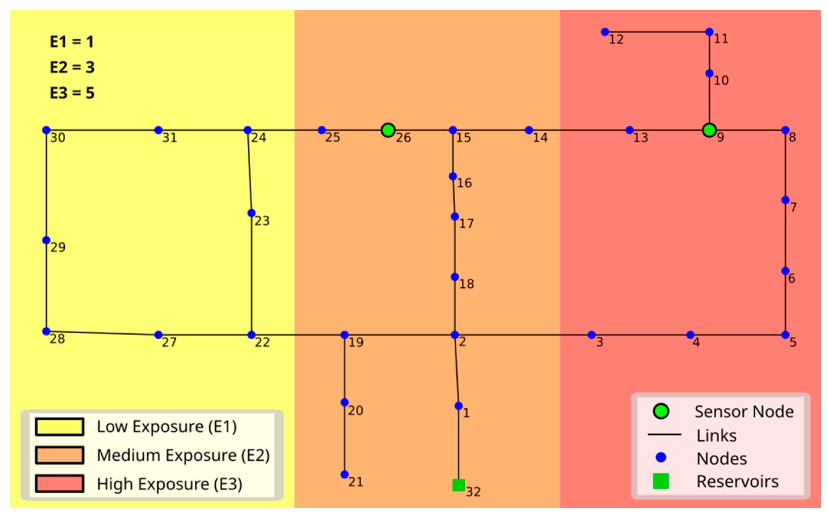
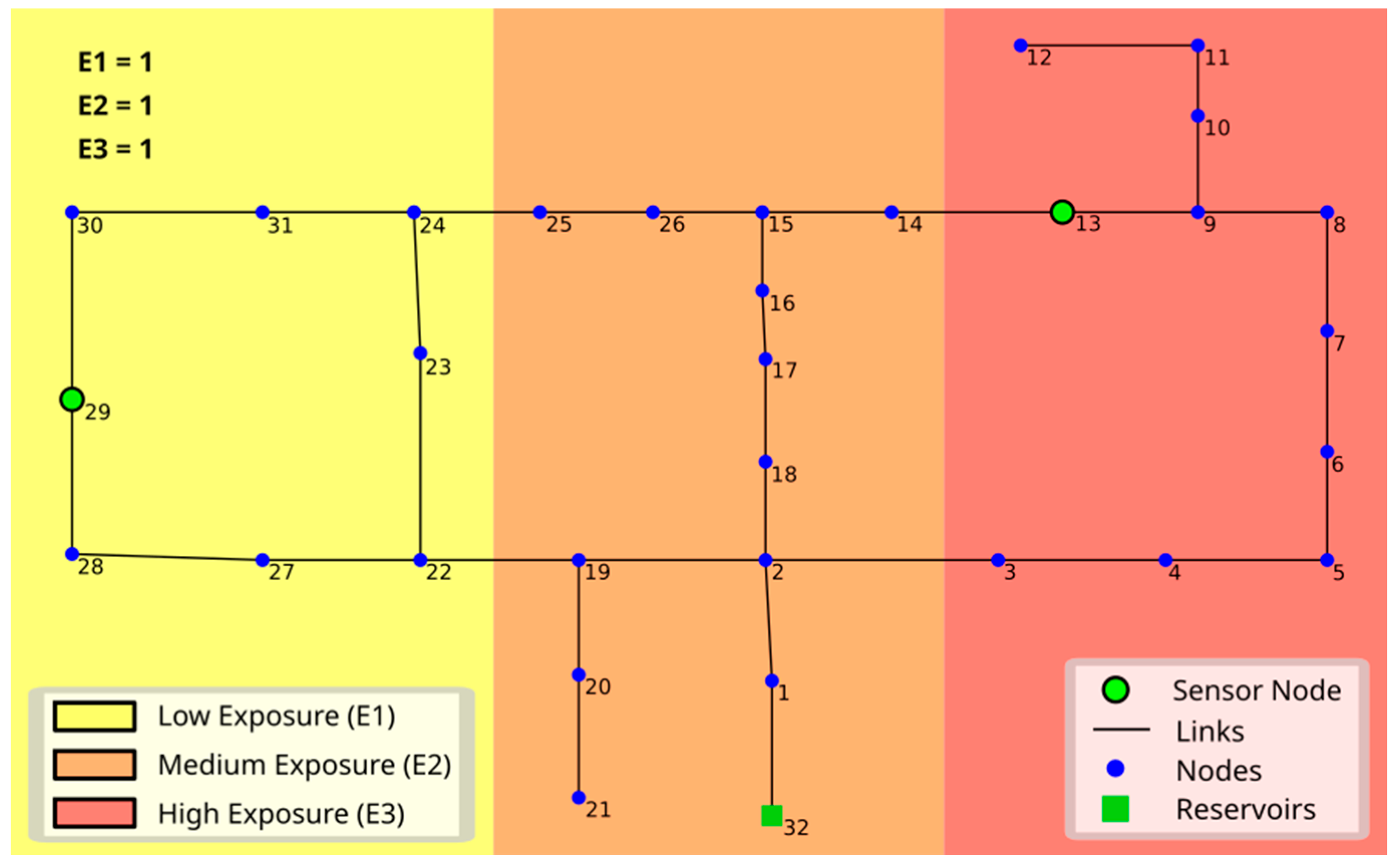
| E1, E2, E3 | 1, 3, 5 | 1, 1, 1 |
|---|---|---|
| Optimal sensor set | 9, 26 | 13, 29 |
| Average localization accuracy | 0.890 | 0.896 |
| Localization accuracy in E2–E3 | 0.896–0.890 | 0.895–0.857 |
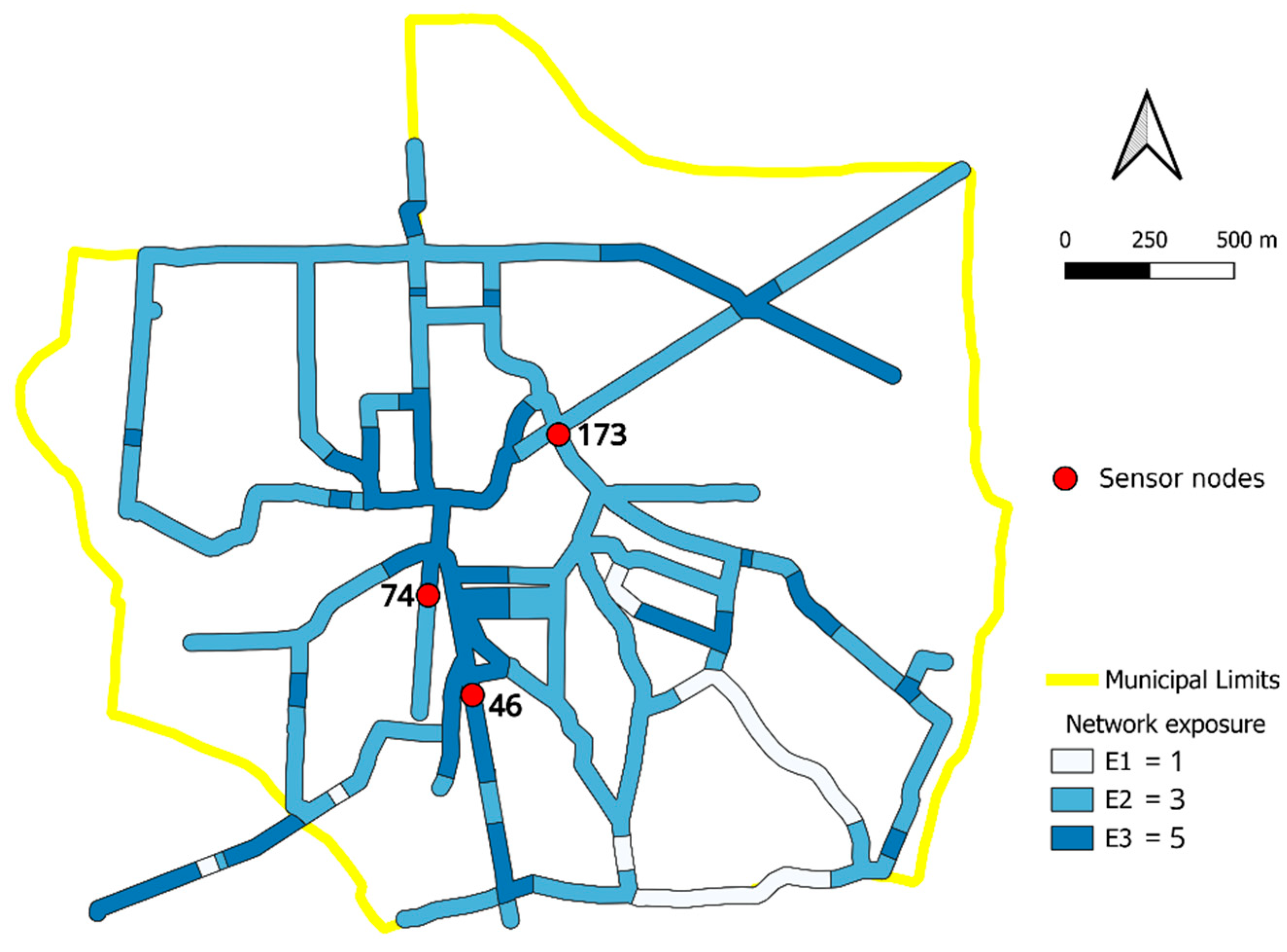
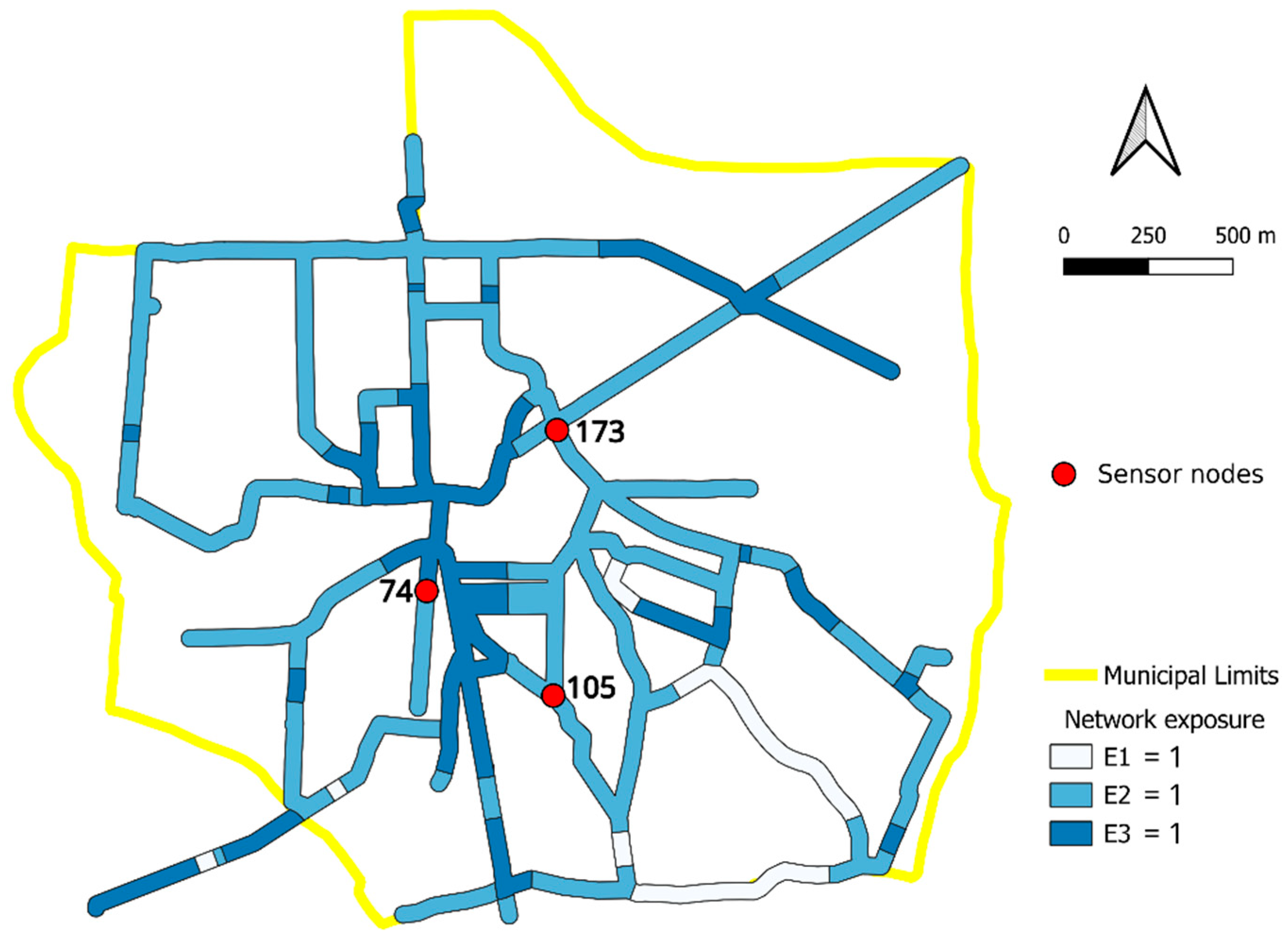
| E1, E2, E3 | 1, 3, 5 | 1, 1, 1 |
|---|---|---|
| Optimal sensor set | 46, 74, 173 | 74, 105, 173 |
| Average localization accuracy | 0.740 | 0.743 |
| Localization accuracy in E2–E3 | 0.700–0.837 | 0.707–0.829 |
| E1, E2, E3 | 1, 3, 5 |
|---|---|
| Optimal sensor positions | 35, 62, 150 |
| Average localization accuracy | 0.735 |
| Localization accuracy in E2–E3 | 0.723–0.867 |
Disclaimer/Publisher’s Note: The statements, opinions and data contained in all publications are solely those of the individual author(s) and contributor(s) and not of MDPI and/or the editor(s). MDPI and/or the editor(s) disclaim responsibility for any injury to people or property resulting from any ideas, methods, instructions or products referred to in the content. |
© 2024 by the authors. Licensee MDPI, Basel, Switzerland. This article is an open access article distributed under the terms and conditions of the Creative Commons Attribution (CC BY) license (https://creativecommons.org/licenses/by/4.0/).
Share and Cite
Medio, G.; Varra, G.; İnan, Ç.A.; Cozzolino, L.; Della Morte, R. Sinkhole Risk-Based Sensor Placement for Leakage Localization in Water Distribution Networks with a Data-Driven Approach. Sustainability 2024, 16, 5246. https://doi.org/10.3390/su16125246
Medio G, Varra G, İnan ÇA, Cozzolino L, Della Morte R. Sinkhole Risk-Based Sensor Placement for Leakage Localization in Water Distribution Networks with a Data-Driven Approach. Sustainability. 2024; 16(12):5246. https://doi.org/10.3390/su16125246
Chicago/Turabian StyleMedio, Gabriele, Giada Varra, Çağrı Alperen İnan, Luca Cozzolino, and Renata Della Morte. 2024. "Sinkhole Risk-Based Sensor Placement for Leakage Localization in Water Distribution Networks with a Data-Driven Approach" Sustainability 16, no. 12: 5246. https://doi.org/10.3390/su16125246
APA StyleMedio, G., Varra, G., İnan, Ç. A., Cozzolino, L., & Della Morte, R. (2024). Sinkhole Risk-Based Sensor Placement for Leakage Localization in Water Distribution Networks with a Data-Driven Approach. Sustainability, 16(12), 5246. https://doi.org/10.3390/su16125246