To determine better ventilation methods, computational fluid dynamics was used in the study, and a numerical model of airflow organization and aerosol diffusion was constructed. The study determined a better ventilation method through the construction of a numerical model. To further optimize better ventilation methods and determine better positions for return air and inlet air, a multi-constraint optimization mathematical model was studied and constructed, and an improved PSO algorithm was designed to solve it.
2.1. Construction of Numerical Models for Airflow Organization and Aerosol Diffusion
To find the safest and most comfortable indoor ventilation method, numerical simulation methods were used to construct numerical models for airflow organization and aerosol diffusion. Based on the indoor airflow organization and aerosol diffusion under different ventilation methods, the study selected the indoor ventilation technologies that need to be optimized in the future. Four indoor ventilation methods were selected for the study, namely mixed ventilation, “air rain” flow field, floor air supply, and displacement ventilation. To simulate different ventilation methods, Computational Fluid Dynamics (CFD) simulations were utilized in the study. CFD simulation can eliminate the influence of uncontrollable factors, simulate multiple situations in a short time, and parameter modification is also very convenient [
16]. For the basic control equation of continuous phase, the Boussinesq hypothesis was adopted to handle the buoyancy caused by temperature difference in the study. The general expression of the continuous phase control equation is shown in Equation (1) [
17].
In Equation (1),
represents the general variable,
represents the Hamiltonian operator,
means the generalized diffusion coefficient,
refers to the generalized source term,
means fluid density,
represents time,
represents gas composition,
is the gravitational acceleration,
is the calculation of partial derivatives,
is the gravity density, and
is the percentage system. The flow characteristics of indoor air are turbulent flow. To numerically simulate turbulent flow, the Reynolds averaging method, which is a non-direct numerical simulation method, was used in the study. The k-ε and k-ω models in the Reynolds-averaged eddy viscosity model are common turbulence models [
18]. To better simulate turbulent flow, the study adopted the k-ε shear stress model that combines the advantages of k-ε and k-ω models. The convective diffusion process of microbial particles in indoor flow fields can be regarded as a gas–solid two-phase flow. To solve the two-phase flow problem, the study adopted the particle tracking method for numerical simulation, which is a discrete dispersed particle model. The motion trajectory equation of a single particle is shown in Equation (2).
In Equation (2),
represents the fluid drag force acting on the particles,
represents the gravity and buoyancy acting on the particles,
represents the additional force acting on the particles,
represents the speed of particle movement,
refers to the speed of airflow movement,
is the densities of particles, and
represents particles,
represents differential operation, and
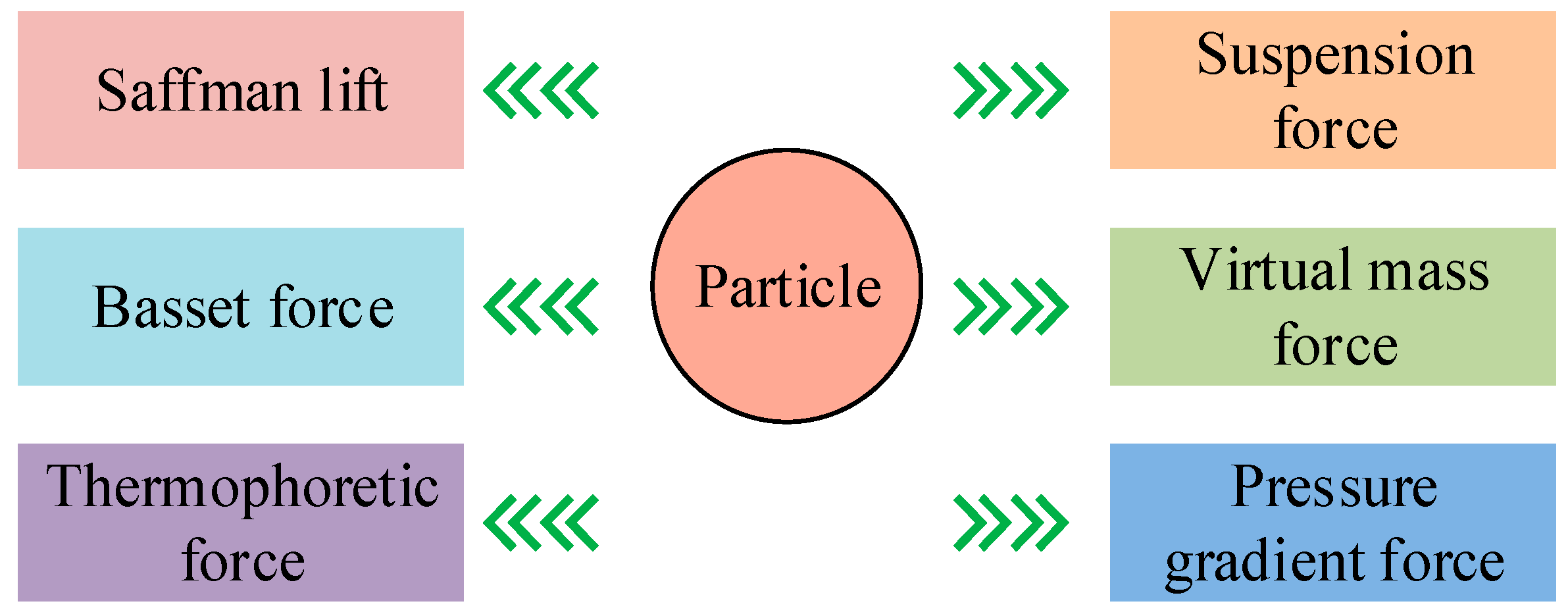
is the symbol of differential operation. The additional force acting on the particles is shown in
Figure 1.
From
Figure 1, it can be seen that the additional forces acting on particles mainly include suspension force, virtual mass force, pressure gradient force, thermal swimming force, Saffman lift, and Basset force. The calculation of suspension force is shown in Equation (3) [
19].
In Equation (3),
represents the particle diameter (simplified as a sphere), and
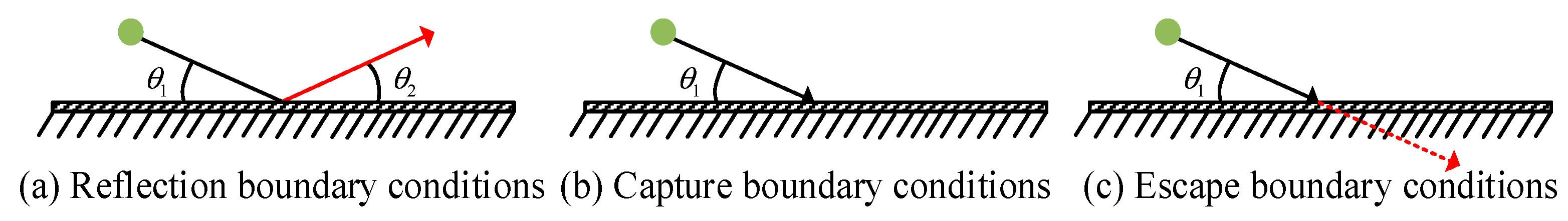
represents suspension force. The model needs to incorporate mixed discrete phase boundary conditions, including reflection boundary conditions, capture boundary conditions, escape boundary conditions, wall jet boundary conditions, wall thin-film boundary conditions, and user-defined boundary conditions. Among them, reflection, capture, and escape boundary conditions are the most important, as shown in
Figure 2.
In
Figure 2,
and
represent the angles of incidence and reflection, respectively.
Figure 2a–c illustrate the boundary conditions for particle reflection, capture, and escape, respectively. For reflection boundary conditions, it is mainly necessary to consider the energy loss caused by non-elastic collision with the wall. When the trajectory calculation is terminated, particles are recorded as “captured”. When a particle encounters an escape boundary, it will “escape”, and trajectory calculation will also stop. The schematic diagram of the numerical calculation physical model is denoted in
Figure 3.
From
Figure 3, it can be seen that the length, width, and height of the numerical calculation physical model are 3.5 m, 2.4 m, and 3 m, respectively. The distance between two human models is 0.5 m, and one person is the source of infection, while the other person is a susceptible person. On the body surface, room floor, ceiling, and tabletop, capture boundary conditions are used in the study, while on the human mouth, air supply outlet, and exhaust outlet, escape boundary conditions are used in the study.
2.2. Design of Improved SVR-PSO Algorithm for Multi-Objective Optimization of Ventilation Methods
To simulate the airflow organization and aerosol diffusion inside the building, a corresponding numerical model was constructed. Based on this numerical model, the thermal comfort and aerosol propagation under different air supply methods were simulated. Based on the simulation results, the study selected a more advantageous “air rain” flow field for further optimization. The specific simulation results will be developed later. The “air rain” flow field can suppress the diffusion of indoor pollutants, but there are also some shortcomings, such as the need for suspended floors and suspended ceilings throughout the house. However, suspended flooring is costly and difficult to clean [
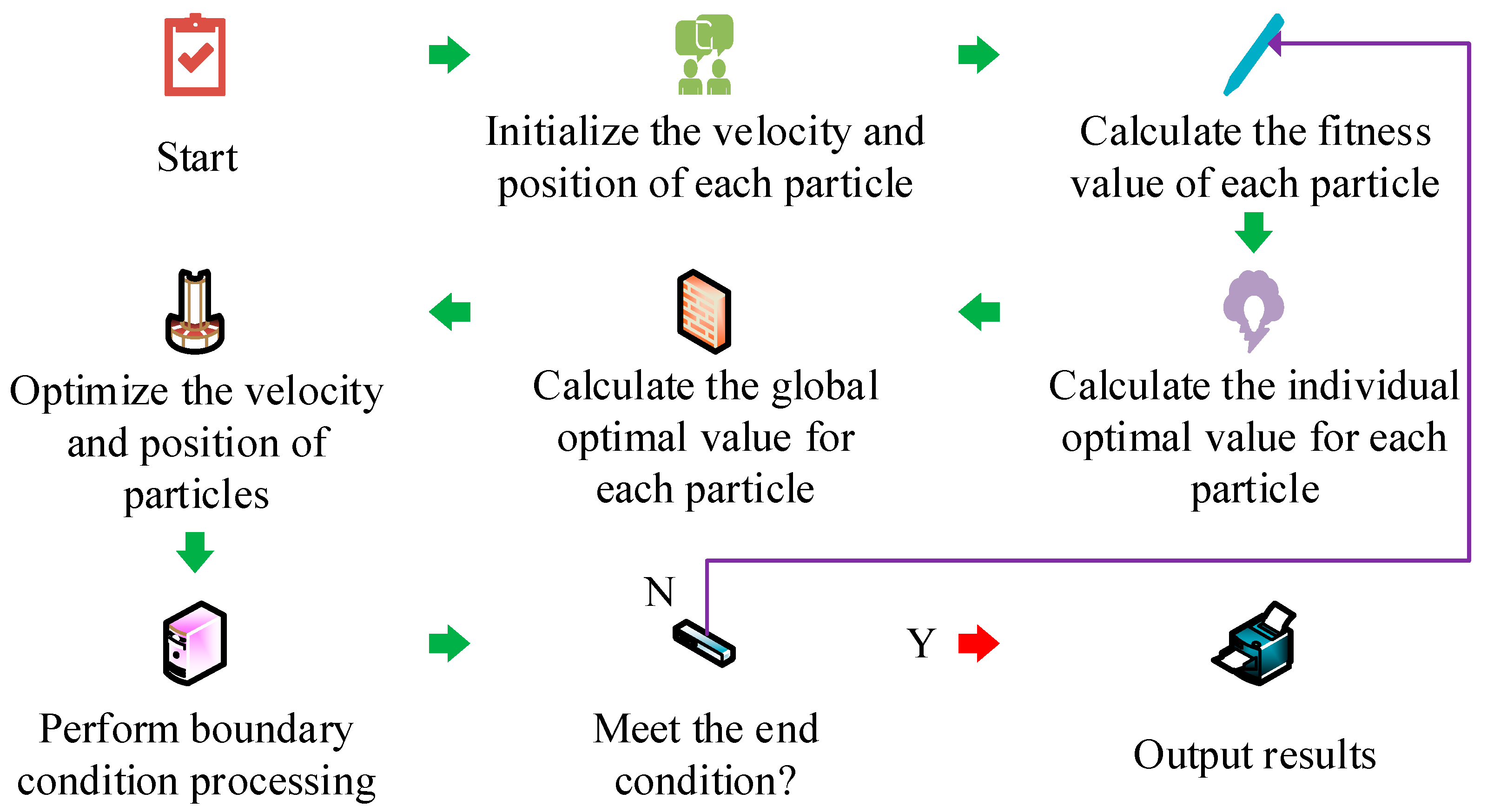
20]. Therefore, the study will conduct multi-objective optimization from the positions of the return air and inlet air. With the development of artificial intelligence, more and more algorithms are being developed to solve real-world problems. PSO has the advantages of simplicity, high accuracy, and fast convergence, and has good advantages in solving practical problems. The main process of the PSO algorithm is shown in
Figure 4 [
21].
From
Figure 4, the first step of the PSO algorithm process is to initialize the velocity and position of each particle, and the second step is to calculate the fitness value of each particle. The third step is to calculate the individual optimal value for each particle, and the fourth step is to calculate the global optimal value for each particle. The fifth step is to optimize the velocity and position of particles, and the sixth step is to perform boundary condition processing. The seventh step is to determine whether the constraint conditions are met. If it is determined to be yes, the output result ends the process. Otherwise, it returns to the third step. However, the PSO algorithm is prone to falling into local optima, so research will optimize it. SVR is an important branch of Support Vector Machine, which can greatly reduce computational cost [
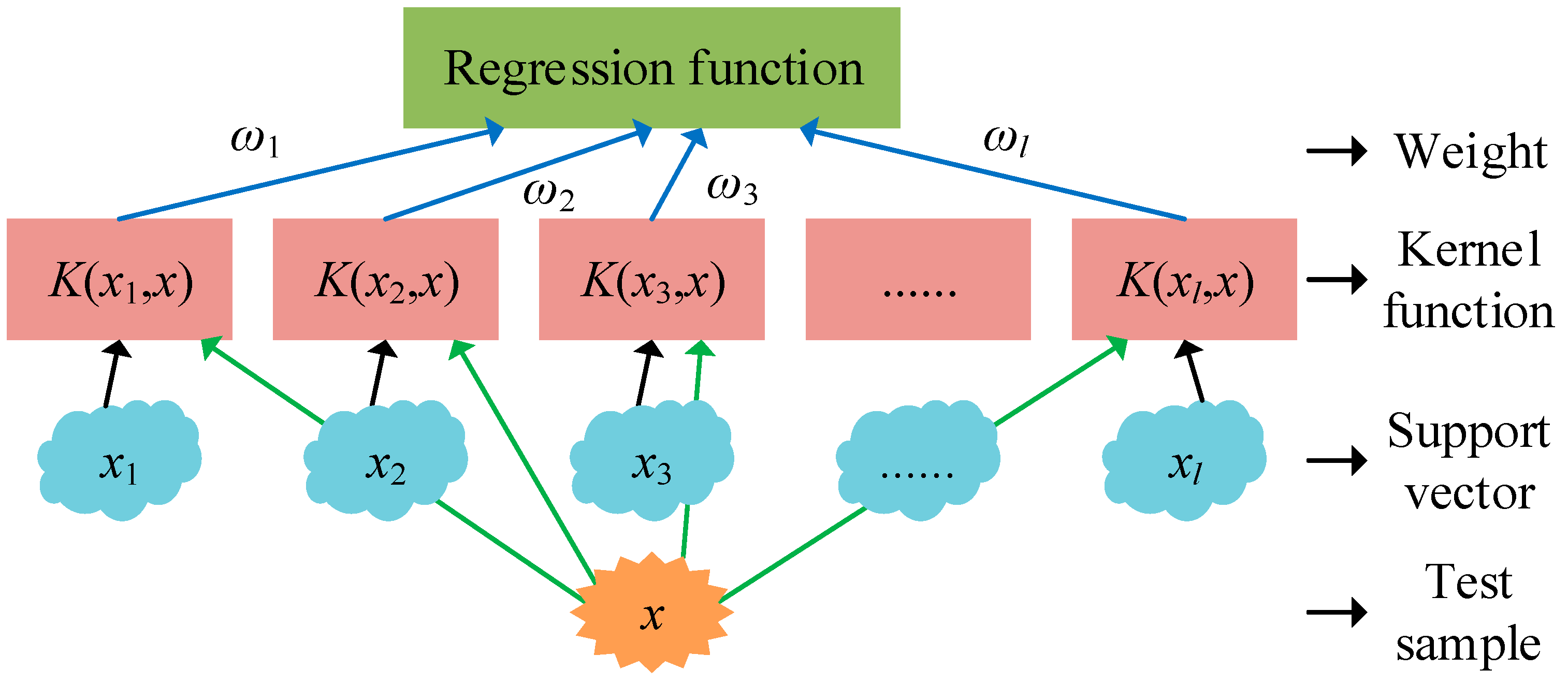
22]. Therefore, the study will use SVR to optimize PSO and form the SVR-PSO algorithm. The main process of SVR is shown in
Figure 5.
From
Figure 5, the main process of SVR involves regression functions, weights, kernel functions, support vectors, and test samples. Among them,
is the input,
is the weight,
represents the serial number, and
is the test sample.
represents the total number of serial numbers. The kernel function used in the study is Gaussian kernel function. The expression of the regression function is shown in Equation (4).
In Equation (4),
represents the threshold. The method of seeking the lowest regression risk in SVR is shown in Equation (5).
In Equation (5),
represents the upper limit training error, and
represents the lower limit training error.
is the regularization penalty term, and
is the
-th.
represents the transpose of weights. To minimize the regression risk in SVR, constraints need to be met, as shown in Equation (6).
In Equation (6),
represents the insensitive loss function, and
is the second input in the kernel function. The general expression of kernel function is shown in Equation (7).
In Equation (7),
represents the kernel parameter of the kernel function, and
and
are both input variables of the kernel function. The final regression function is shown in Equation (8).
In Equation (8),
and
are both Lagrangian coefficients, and their values are ≥ 0.
is the kernel function.
and
are the input values in the kernel function, where
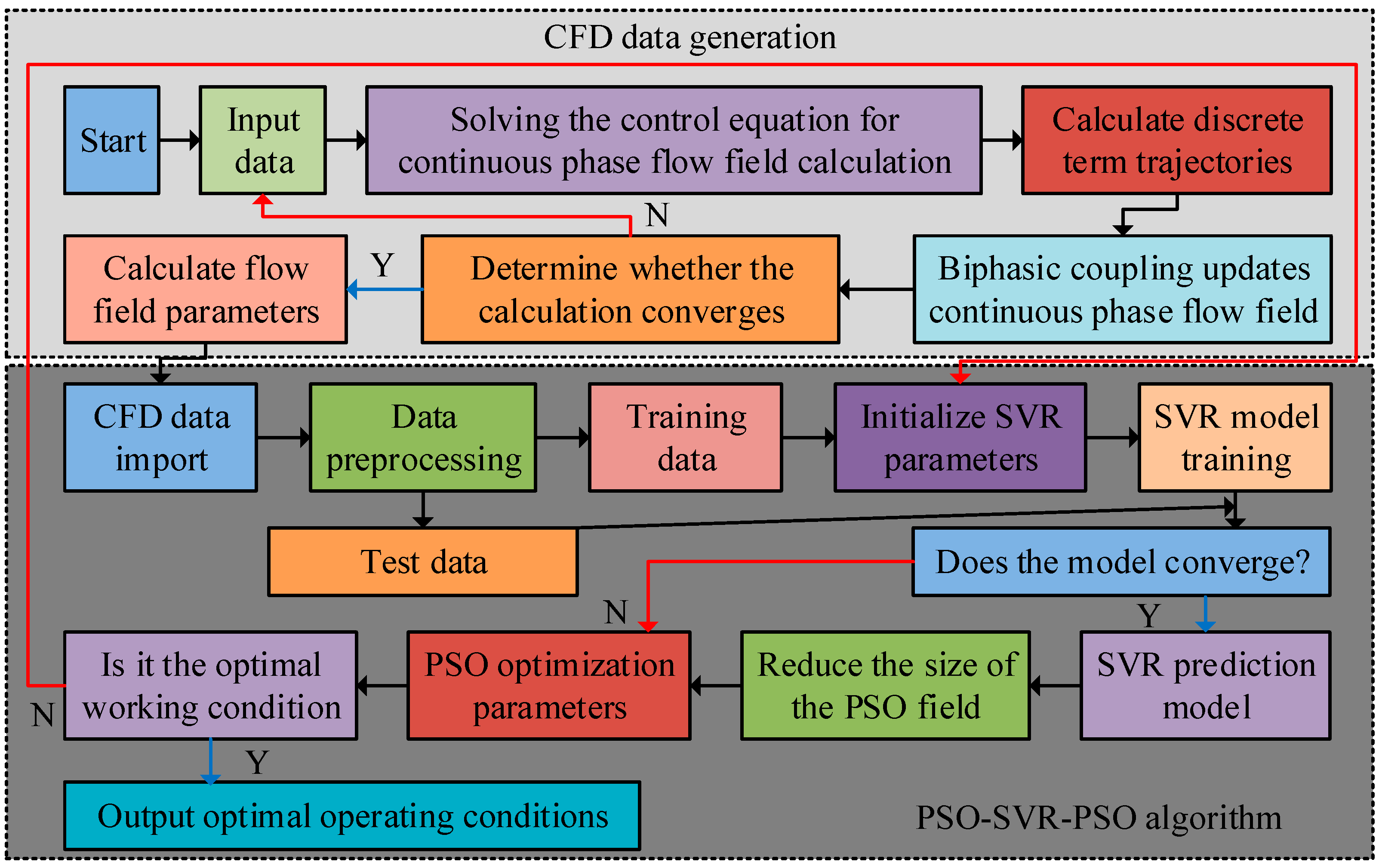
is the ordinal. To better leverage the performance of the SVR-PSO algorithm, research optimized it to form the final PSO-SVR-PSO algorithm. The specific optimization approach is to first use the SVR-PSO algorithm to construct a predictive model for CFD data, followed by PSO iterative calculation to perform multi-objective optimization on the ventilation mode. The optimization process of the PSO-SVR-PSO algorithm is denoted in
Figure 6.
From
Figure 6, the optimization of the PSO-SVR-PSO algorithm is mainly divided into two parts. The first part is CFD data generation, and the second part is the specific process of the algorithm. The first step in generating CFD data is to input the data, and the second step is to solve the control equation for the continuous phase flow field calculation. The third step is to calculate the trajectory of the discrete term, and the fourth step is to update the continuous phase flow field through two-phase coupling. The fifth step is to determine whether the calculation converges. If it converges, it will calculate the flow field parameters. Otherwise, it will go back to the first step. The first step in the specific process of the PSO-SVR-PSO algorithm is to import CFD data, and the second step is to preprocess the data. The third step is to divide the data into training data and testing data. The fourth step is to initialize the SVR parameters. The fifth step is to train the SVR model, and the sixth step is to combine test data to determine whether the model converges. If convergence occurs, it will output the SVR prediction model, then reduce the size of the PSO domain and optimize the parameters for PSO. Otherwise, PSO optimization parameters will be directly carried out. The seventh step is to determine whether it is the optimal working condition. If it is determined to be the optimal working condition, it will output the optimal working condition. Otherwise, it will go back to the fourth step. For the multi-constraint optimization of ventilation methods, the evaluation criteria used in the study involve infection probability, thermal comfort, energy utilization coefficient, and velocity non-uniformity coefficient. Heat comfort measures used the Predicted Mean Vote and Predicted Percentage Dissatisfied (PMV-PPD) indicators. The solution of Predicted Mean Vote
is shown in Equation (9).
In Equation (9),
represents the metabolic rate of the human body, and
represents the abbreviation of the formula. The specific expansion of
is shown in Equation (10).
In Equation (10),
denotes the mechanical work performed by the human body, and
represents the correlation between the surface coverage area coefficient of the human body and the thermal resistance of the clothing.
denotes the surface temperature of human clothing, while
represents the average radiation temperature.
denotes the surface heat transfer coefficient between indoor air and human clothing, and
represents the air temperature within the range of human activity.
is the partial pressure of water vapor in the vicinity of the human body.
represents human clothing, and
represents the appearance of human clothing. The calculation of
is shown in Equation (11).
In Equation (11),
represents the thermal resistance of human clothing. The calculation of
is shown in Equation (12).
In addition, the calculation of
is shown in Equation (13).
In Equation (13),
represents the indoor airflow velocity. The calculation of energy utilization coefficient
is shown in Equation (14).
In Equation (14),
represents the exhaust temperature,
represents the average temperature of the indoor human activity area, and
represents the supply air temperature. The study normalized and weighted four different evaluation criteria. The expression of the multi-constraint optimization mathematical model
of the PSO-SVR-PSO algorithm is shown in Equation (15).
In Equation (15), , , , and represent the objective functions of the thermal comfort index PMV-PPD, infection probability, energy utilization coefficient, and velocity non-uniformity coefficient, respectively.


