Abstract
Quick post-disaster emergency response of highway bridge networks (HBNs) is vital to alleviating the impact of disasters in affected areas. Nevertheless, achieving their emergency response resilience remains challenging due to the difficulty in accurately capturing the response capacity of HBNs and rapidly evaluating the damage states of regional bridges. This study delves into the emergency response, seismic resilience, and recovery scheduling of HBNs subjected to frequent yet mostly ignored moderate earthquakes. Firstly, the feasibility of intelligent methods is explored as a substitute for nonlinear time-history analysis of regional bridges. Subsequently, for realistic modeling of post-disaster HBNs, a decision tree model is developed to determine potential traffic restrictions imposed on damaged bridges. Moreover, their emergency response functionalities are thoroughly investigated, upon which a comprehensive multi-dimensional resilience metric vector is proposed. Finally, the proposed methodologies are applied to the Sioux Falls HBN as a case study, revealing a decreasing mean value and increasing deviation values in the long term. The results are expected to provide important theoretical and practical emergency response guidance.
1. Introduction
During urbanization and globalization, a substantial number of transportation infrastructures have been constructed worldwide [1]. Among them, highway bridges play a critical role [2]. For example, by the end of 2022, there are a total of 1.03 million highway bridges and 92 thousand railway bridges in China. Situated in regions prone to seismic activity of the Eurasian Plate and the Circum-Pacific Seismic Belt, these bridges are at risk of seismic damages. Regrettably, the effects of moderate and small-scale earthquakes tend to be underestimated due to their lower immediate damage. However, given their higher frequency—numbering in the hundreds annually—and the necessity for cities to promptly return to normalcy after such events, it is crucial for emergency response measures and regular operations to seamlessly coexist.
In fact, the advancements in modern seismic design standards considerably decrease the collapse probability of bridges, even under strong earthquakes with magnitudes (Mw) larger than 7.0. However, recent earthquakes underscore that bridges remain vulnerable under moderate earthquakes. For instance, the Lushan earthquake (Mw = 6.6) in 2013 [3] and Luding earthquake (Mw = 6.8) in 2022 [4] caused damage to 440 bridges and 103 bridges, respectively, not only resulting in enormous economic losses, but also impeding restoration efforts. To make informed decisions on emergency response, it is imperative to (1) capture the seismic damages and (2) understand the related outcomes of bridges, especially within the critical post-earthquake “Golden 72 h” [5]. Generally, regional bridges can only fulfill transportation functions when cooperating with highway segments into a highway bridge network (HBN) [6]. They exhibit significant variations in site conditions, structural types, construction ages, service environments, etc. Coupled with inherent uncertainties, it is extremely difficult to account for all the influencing factors, making it intricate to predict the seismic responses of regional bridges [7,8].
Traditional seismic analysis methods were primarily developed for individual structures, relying on post-disaster investigations, experts’ opinions, numerical simulations, or structural health monitoring (SHM), etc. While these approaches provide valuable insights into the seismic performance of structures, their complexity and computational demands limit their effectiveness or accuracy when directly applied to region-scale bridges, each with unique characteristics and conditions [9]. For instance, the current SHM techniques require numerous sensors and data acquisition devices [10]. Numerical simulations based on finite element models (FEMs) cannot be easily conducted due to the enormous computational cost, especially when it comes to large-scale structures [11]. To address these defects, several simplified methods based on statistics or intelligent algorithms have been specifically custom designed for regional bridges [12,13,14]. They can quantify the probability in certain damage states of structures in terms of fragility curves, based on experts’ opinions, test data, or numerical results, etc. [15,16,17,18]. For example, HAZUS generated fragility curves for bridges across various groups. With the advancement of intelligent algorithms, artificial neural networks (ANNs), decision trees (DTs), etc., have exhibited superior nonlinear learning performance over traditional methods. In the case of available sufficient data, ANNs can model complex relationships between input parameters and structural behaviors (e.g., dynamic response [19] and hysteresis [20]) with high accuracy. DTs, on the other hand, can identify key influencing factors through segmenting data into subsets, such as to predict the seismic behaviors like damage states of structures [17,21]. Compared with traditional methods based on predefined equations and models, these machine learning-based methods are data driven, and require no prior knowledge, making them more promising for region-scale seismic analysis.
On the other hand, for safety, preventive traffic restrictions will be imposed on damaged bridges, potentially obstructing rescue and evacuation efforts over the HBN [22]. Upon becoming aware of an emergency, the situation needs to be quickly assessed to determine the type and scope of the emergency. To capture updated disaster information, various emergency response systems have been developed worldwide, such as the Global Disaster Alert and Coordination System (GDACS, www.gdacs.org accessed on 1 June 2016). However, most of the existing emergency responses lack explicit decisions based on historical emergency response events, which is necessary for realistic emergency response modeling [23]. This is because earthquakes occur without warning, leaving little time for comprehensive planning [24]. Limited information leads to decision making under incomplete knowledge, increasing the risk of errors. Processing and synthesizing this vast amount of information in real time poses a significant challenge. Moreover, large-scale bridge maintenance and repairing efforts are bound to impede highway traffic and economic development [25].
Resilience has become increasingly popular owing to its ability to comprehensively account for a system’s robustness, rapidity, vulnerability, etc., in the recovery process [26,27]. Currently, resilience studies mainly focus on the holistic functionality and unexpected societal events under extreme disasters. Hosseini et al. [28] proposed a probabilistic model to evaluate the network resilience of urban road networks. Kiremidjian et al. [29] evaluated the seismic risk of transportation networks in terms of direct economic losses of bridges and indirect travel delays. The results demonstrated that the rare earthquakes with Mw of 7.0 contribute more to seismic loss than the frequent earthquakes with smaller magnitudes (less than 6.0) in the SFBR. Nevertheless, post-earthquake investigations indicated that moderate earthquakes also tend to incur serviceability deterioration of HBNs [30]. Even if structural damage may not be substantial, the lack of coordinated action of highway administrators may increase drivers’ insecurity and distress [31,32]. This will impede the operation of the HBN, further resulting in additional injuries and losses. In spite of these facts, to the best of the authors’ knowledge, there is limited literature on the emergency resilience of HBNs.
Recognizing the gap in current studies, this study aims to devise a rapid emergency response resilience assessment methodology for HBNs under moderate earthquakes. It applies an inter-disciplinary approach, combining FEM, intelligent algorithms, and traffic flow simulations. In the following sections, Section 2 describes the flowchart of the proposed methodologies. Section 3 provides an ANN-based method for a real-time seismic assessment of regional bridges, which is employed to capture their recovery processes. Additionally, in Section 4, a DT-based approach is to determine potential responses using historical emergency data after extreme events. A comprehensive resilience vector is proposed for evaluating the emergency response of HBNs in Section 5. Finally, the seismic emergency response resilience of the Sioux Falls HBN is investigated using the developed ANN and DT models, demonstrating their effectiveness.
2. Intelligent Resilience Analysis Framework of HBN
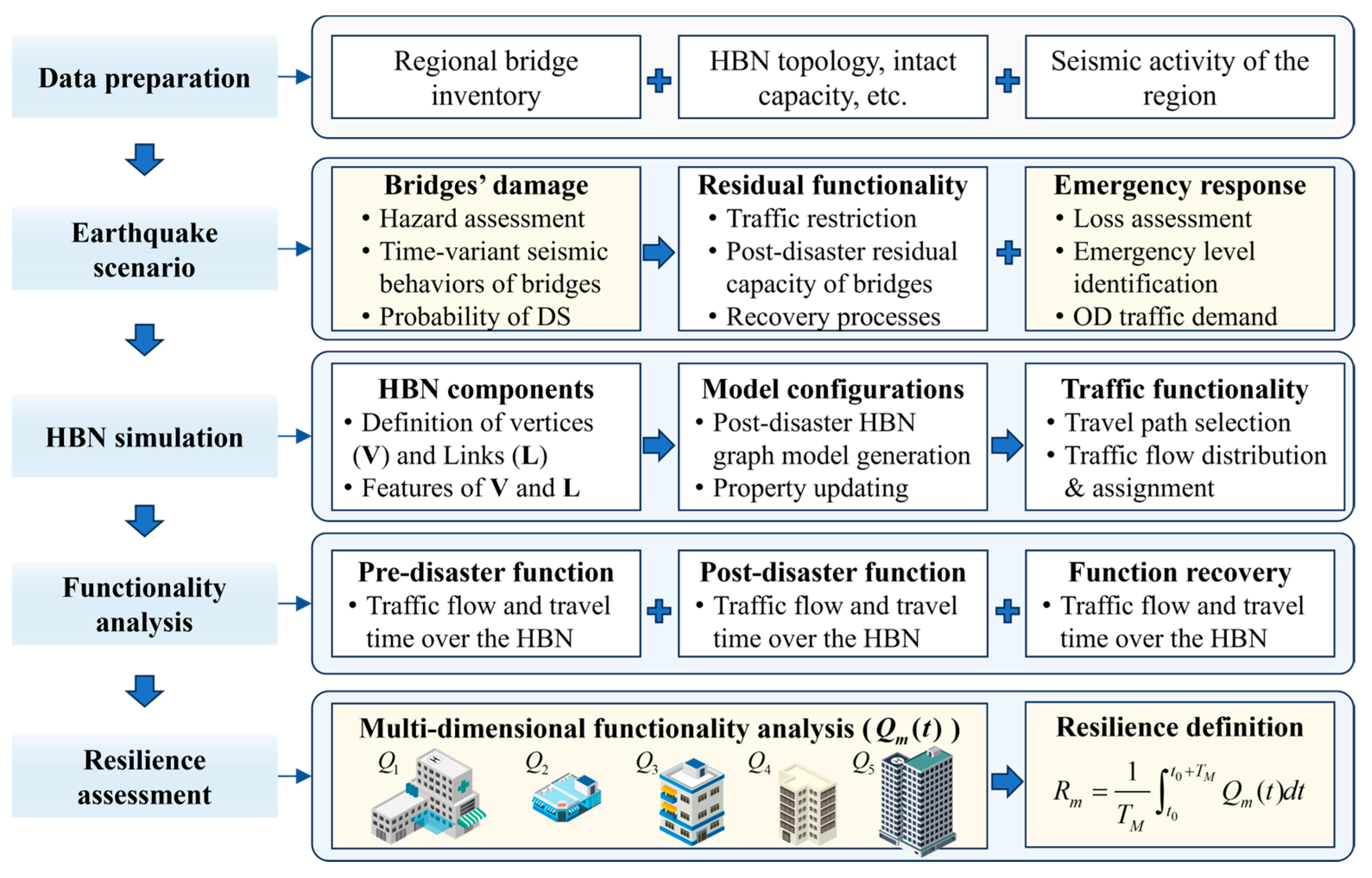
The seismic emergency response of HBNs depends on a broad spectrum of factors. To comprehensively evaluate their resilience, a framework is proposed herein. As shown in Figure 1, it accounts for the probabilistic seismic hazards, post-disaster scenarios of bridge damages and emergency responses, functionality recovery and resilience, etc. A set of scenarios over the long term will be used to capture the time effects. The first step is to identify the bridge inventory (including structural type, geometrical size, material properties, and reinforcement arrangements), HBN configurations (e.g., links, travel capacity), and seismic activity of the region. With these basic data, the seismic resilience of HBNs can be quantified by the following four modules:
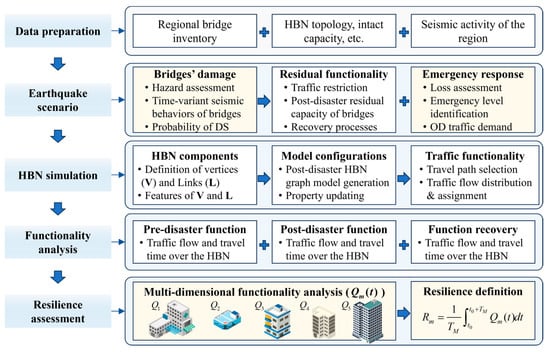
Figure 1.
Flowchart and main modules.
- (1)
- Earthquake scenario: The seismic effects can be reflected by three interconnected branches, namely bridges’ damage, residual functionality, and emergency. The first two parts aim to provide a reasonable estimate of the post-disaster traffic-carrying traffic capacity of bridges, while the last one contributes to the traffic demand determination.
- (2)
- HBN simulation: A mathematical graph model G with vertices (V) and links (L) can be generated to represent the topology of the HBN. Along with the post-disaster travel capacity and traffic demand, the functionality of each link can be determined following the traffic flow distribution and assignment procedure.
- (3)
- Functionality analysis: Based on modules (1) and (2), the emergency response functionalities of the HBN in pre-disaster, post-disaster, and recovery processes can be quantified in terms of traffic flow and travel time. After investigating how a typical city responds to and recovers from earthquakes, the emergency response functionalities of HBNs are quantified in terms of rescue, evacuation, repair, material allocation, and others. Then a multi-dimensional functionality vector is proposed.
- (4)
- Resilience assessment: Adhering to the resilience definition, the resilience of a HBN can be quantified by integrating the time-variant functionality over the recovery period. To account for the inherent uncertainties stemming from structural properties, ground motions, and other factors, Monte Carlo simulation (MCS) would be applied to iterate through the aforementioned steps.
Since many parts of them (in white boxes) have been extensively investigated in prior research, this study mainly focuses on addressing the challenges in the (a) real-time seismic assessment of regional bridges, (b) realistic emergency response decision, (c) multi-dimensional resilience assessment of HBNs.
3. Rapid Seismic Assessment of Regional Bridges
A comprehensive seismic assessment of bridges should indeed incorporate diverse characteristics that significantly impact their seismic behaviors. Traditional FEM-based techniques simulate their mechanical behaviors through a series of interconnected component elements. However, the identification of parameters for various structural components and dynamic analysis processes causes an enormous computational cost, especially when applied to regional bridges with large inherent uncertainties. It is not readily available in the immediate aftermath of an earthquake. To address that, simplified methods need to consider these characteristics and ensure that their effects are adequately captured.
3.1. Data-Driven Seismic Fragility
Fragility curves in the context of bridges typically refer to the condition probability of their components ci being in a certain damage state given a specific intensity measure (IM) of the ground motion excitation, i.e., [7]. They can be determined by whether the seismic demands exceed a certain limit state , namely [33]. The pre-defined limit state of describes the extent of damage that a bridge can withstand before it is considered unsafe or non-functional. Consequently, the key to bridge fragilities lies in the determination of . Although spectral acceleration corresponding to the fundamental period of the bridge is more effective than other indicators, due to the need for modal analysis of the fundamental periods of regional bridges, the fundamental periods of different bridges are inconsistent. Additionally, regional bridges have a wide distribution, leading to significant differences in seismic intensity characteristics experienced by each bridge. This paper adopts the spectral acceleration corresponding to a period of 1.0 s (Sa), which is commonly used in engineering [34].
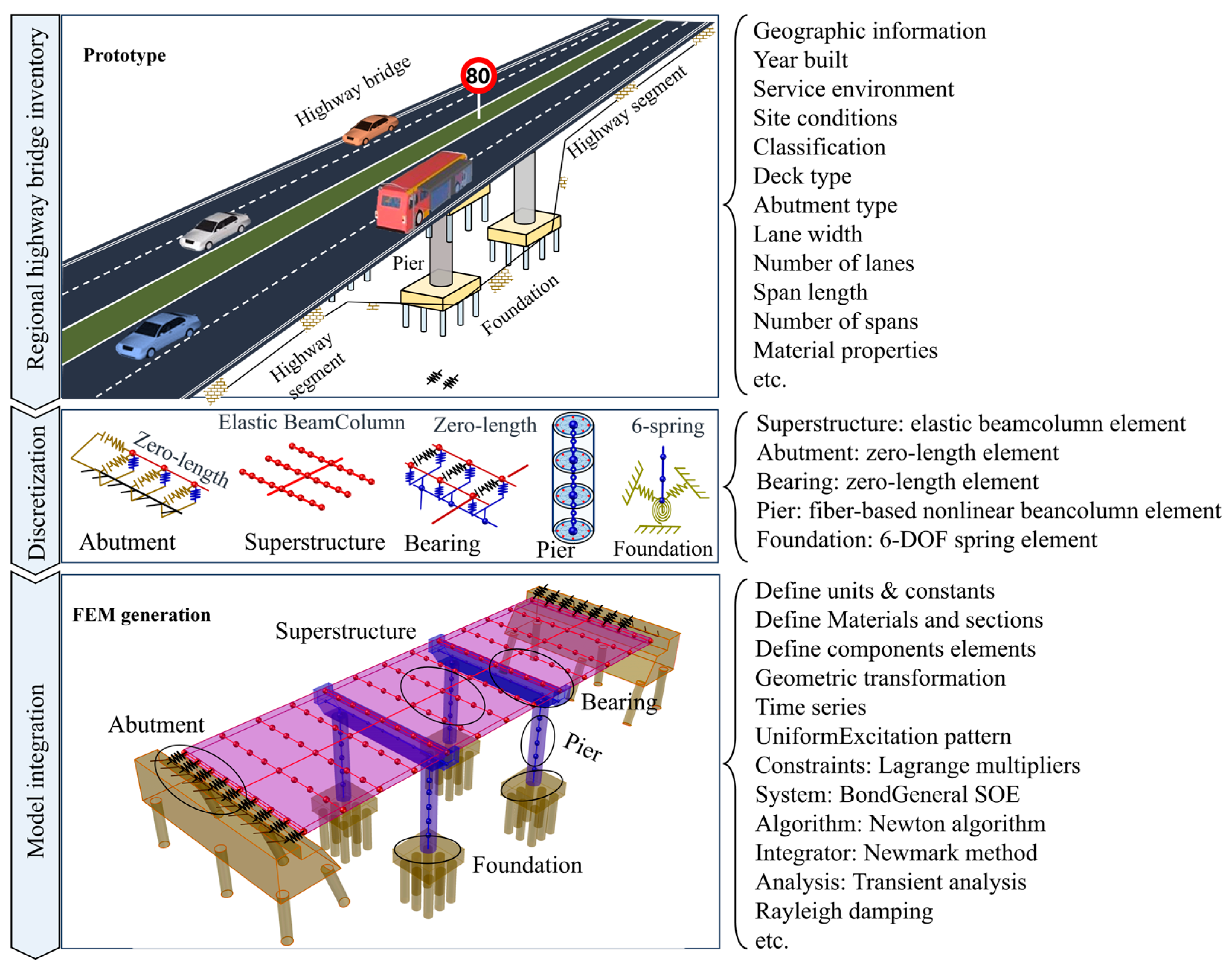
A data-driven seismic fragility surrogate method is proposed in this study ( denote the ANN model). Furthermore, the regional highway bridge inventory should be first identified, including its geographical information, service environment, and structural properties. As illustrated in Figure 2, this study focuses on the commonly used girder-type highway bridges; other types of bridges can be simulated following the same procedures. A typical girder-type highway bridge consists of superstructure (deck and girder), bearing, abutment, pier, and foundation. Subsequently, based on the mechanisms of bridge components, corresponding elements will be selected. By referring to the relative literature [17,35], the superstructure can be simulated by an elastic beam column element with distributed mass, representing the stiffness, strength, and mass of decks and girders [33]. As for connection components, they can be modeled by zero-length elements with suitable materials. For example, the abutment, bearing, and foundation elements of girder-type highway bridges contain suitable hyperbolic–hysteretic–elastomeric bearing plasticity impact material [36], hysteretic–elastomeric bearing plasticity [33], and 6-DOF spring materials, respectively. Finally, a detailed three-dimensional FEM, including geometric nonlinearities like P- effects and Rayleigh damping, can be generated for bridge by integrating these elements.
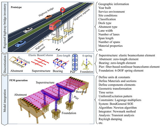
Figure 2.
FEM generation and mathematical characterization of a typical highway bridge.
Consequently, the influencing characteristics of bridge i are determined as the model parameters of critical components, as follows:
where BN, BL1, and BW denote the span number, standard span, and deck width, respectively; BST, BA, and BI represent the superstructure type, section area, and inertia moment, respectively; BNb and BKb are the number and stiffness of bearings, respectively; BAT are the abutment type; Bpn, Bh, BDc, and Bpl denote the number of columns per pier, pier height, pier diameter, and longitudinal reinforcement ratio, respectively. Other parameters can be derived by (1) the above parameters, for example, the superstructure mass can be estimated as Bpc × BL1 × BA (Bpc is the concrete density); (2) MCS according to their engineering distribution, such as Bpc following uniform distribution U(2250, 2750) kg/m3, steel and concrete strength values following lognormal distribution LN(5.81, 0.1) MPa and normal distribution N(30, 4.5 MPa, respectively. For more details, please refer to [21,37].
3.2. Bridge Seismic Fragility Database Preparation
As mentioned above, the primary process of seismic damage analysis for bridges, which involves establishing a numerical model based on bridge characteristics , conducting incremental dynamic analysis (IDA) and probabilistic seismic demand (PSDA) for seismic responses and fragilities. To substitute for time-consuming numerical simulations, a data-driven surrogate seismic fragility model needs to be developed. For that purpose, a database with abundant bridge characteristics is crucial.
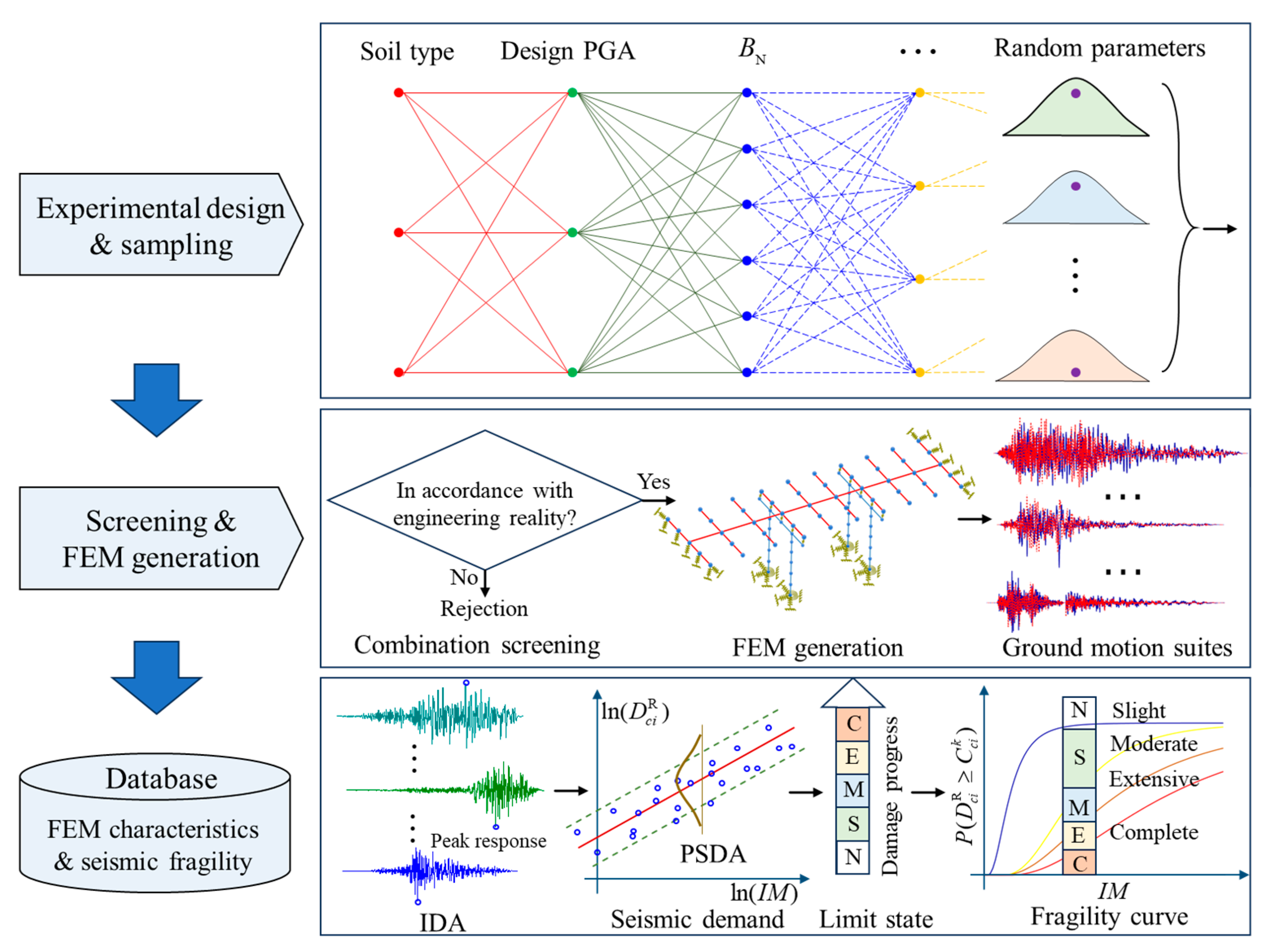
Figure 3 depicts the procedure for developing a seismic fragility database of bridges. A series of bridge characteristics were generated according to the potential engineering ranges of . For example, the standard span length values of slab bridges and box-girder bridges are in the range of 5 m~15 m and 15 m~40 m, respectively. The potential span number is 2~7. The pier heights vary from 3.0 m to 9.0 m, with corresponding diameters ranging from 0.3 m to 2.0 m. The number of columns per pier is in the range of 1~5. They are paired with random parameters sampled according to their probability distributions, as outlined in Table 1. Subsequently, these combinations undergo a checking step; anyone inconsistent with engineering reality would be rejected.
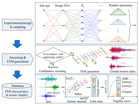
Figure 3.
Schematic illustration of surrogate fragility modeling.

Table 1.
Random parameters and their engineering probability distributions [38,39].
The remaining qualified combinations are then used to generate FEMs that are paired with ground motions for seismic assessment. A total of 1548 urban highway bridge specimens, covering the common engineering range and combination of bridges, are designed herein. After conducting time-history analysis using ground motions, the seismic demands and damage states of these bridges can be quantified.
To consider the time-frequency characteristics of seismic motion, the 160 ground motion records for seismic analysis of transportation systems are adopted herein [40]. They cover the influencing characteristics of broadband ground motions at various sites, with Mw ranging from 4.3 to 7.9. Each ground motion consists of two orthogonal components in horizonal directions, which were employed in IDA for bridges. Typically, acceleration time histories rather than displacements were imposed to the base nodes of the FEM, effectively simulating the seismic forces and their impact on the structural response. This method ensures a realistic representation of seismic activity and its effects on the bridge. Specifically, each suite of ground motions was scaled to a peak ground acceleration (PGA) of 0.1 g, 0.3 g, 0.7 g, 1.0 g, and 1.3 g. This scaling allows the bridge database to cover a wide range of seismic intensities, ensuring the developed ANN model’s generation ability. The Open System for Earthquake Engineering Simulation (OpenSEES) software (version: 3.6.0) [41] is adopted herein. It provides a versatile and robust platform for numerical simulation in earthquake engineering research and practice. The peak seismic responses of critical bridge components are selected as seismic demands, as illustrated in Table 2. For example, the curvature ductility of pier columns is utilized herein. Finally, by comparing their seismic demands and capacities, the seismic fragility curves of bridges can be established.
Table 2.
Critical seismic demand parameters and limit states [33].
3.3. Training and Validation
A data-driven seismic fragility model essentially means to directly relate with , bypassing the need using numerical analysis. Considering the significant difference in the ranges and units of both and (ci = 1,2,3,…,6), they are first normalized within the range of [0,1] by
where and denote the minimum and maximum value of the j-th feature of all bridge specimens, respectively; and are the minimum and maximum value of the ci-th seismic demands of all bridge specimens, respectively.
Therefore, 14 input neurons (i.e., bridge characteristics and IM) and 6 output neurons are determined. While deep neural networks like convolutional neural networks (CNN) and recurrent neural networks (RNN) excel in nonlinear representation capabilities, they require substantial training samples. The scale of the model parameters to be determined can be extremely immense, even reaching tens of thousands or billions. Moreover, CNNs are suitable for mesh data, while RNNs are more adept at temporal feature data. A three-layer fully connected ANN is suitable for regression analysis, with few model parameters and strong controllability. According to Kolmogorov’s theorem, this network can approximate any continuous function.
Firstly, 80% and 20% of the bridge samples were randomly divided into training and testing sets. To avoid overfitting of the model and ensure generalization performance, the K–fold cross validation method is adopted, which randomly divides the training set samples into K equal parts and takes turns as the validation set to validate the model trained with the remaining K–1 ones. Each data point is used for validation exactly once and for training Kv1 times, ensuring that the model is tested against all available data while still being trained on a substantial subset of the data in each iteration. In this study, the choice of K = 10 is adopted for the following reasons: (1) bias-variance trade-off: fewer folds, such as 5-fold, might result in higher variance, while more folds, such as 20-fold, can increase the bias, as each training set becomes smaller; (2) computational efficiency: 10-fold cross-validation is computationally efficient, allowing for a thorough evaluation of the model without excessively increasing the computational burden. Then, the data of each neuron are weighted and activated and passed to the next layer until the output layer. The weights of each connecting layer are adjusted based on the error between the predicted value and the actual value, and the process is repeated until the termination condition is met (loss less than 10−3 or iteration number reaches 103). The performance of the established model is evaluated using root mean square error () and goodness of fittness (), as follows:
where denotes the total sample number; is the average of all samples.
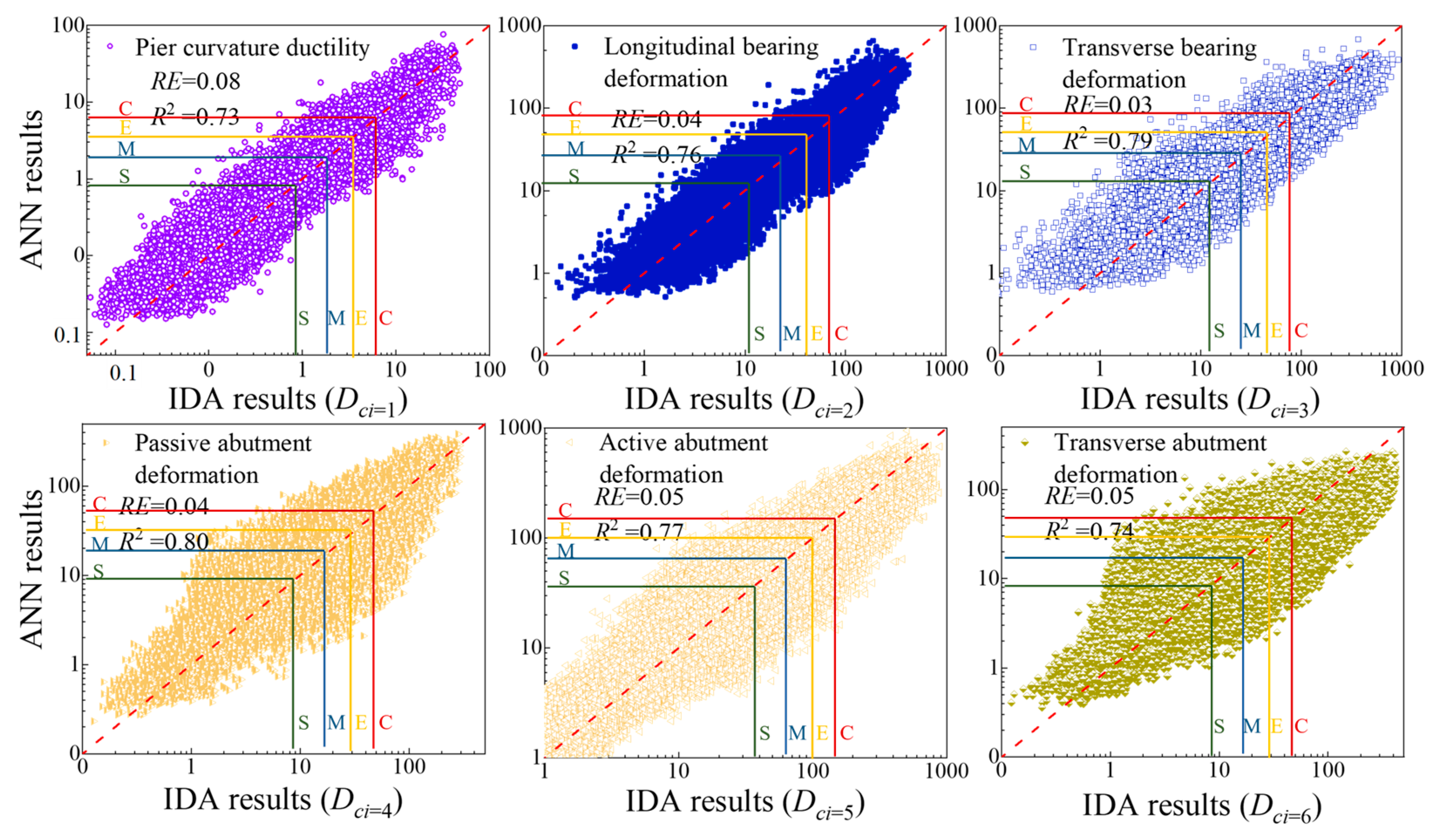
After training, the optimal number of hidden layer neurons was ultimately selected as 50. The test results of this model are shown in Figure 4. As can be seen, the values of seismic demand prediction for the key components of bridges are between 0.03 and 0.08, and the values are between 0.73 and 0.80. It can be seen that the ANN model can replace the IDA analysis method to accurately evaluate the seismic damage status of bridge structures. Moreover, once trained, the surrogate model no longer requires training. According to the predicted seismic demands, the damage states of components can be captured by comparing with limit states. As mentioned in Section 3.1, the fragilities of the bridge, namely the probabilities of bridges being in a certain damage state, can then be determined, . In this study, the damage states are divided into five groups: none (N), slight, moderate (M), extensive (E), and complete (C). The figures in Figure 4 illustrate that the ANN-based fragilities compare well with their IDA-based counterparts.

Figure 4.
Surrogated versus modeled seismic demand plot.
Consequently, the ANN model for seismic demand assessment can provide bridge damage results within 1 s, achieving rapid seismic evaluation of regional bridges. In contrast, the IDA method requires several hours to analyze a single bridge, highlighting the superiority of ANN methods in terms of computational cost.
3.4. Normalized Recovery Process of Damaged Bridges
The functionality of bridges primarily revolves around their traffic capacity (TCB), maximum traffic speed (TSB), and other aspects, all of which are tied to the connectivity of the surrounding roads. In response to seismic damage on bridges, safety measures will be enacted to safeguard motorway users. These precautions might involve lane closures, partial or complete bridge shutdowns, and the imposition of speed limits. While these proactive measures are crucial for minimizing hazards and ensuring the safety of all motorists on the affected roadway, it is important to acknowledge that they will inevitably impact the traffic capacity of bridges. This can lead to traffic congestion and related issues.
The traffic restrictions (TRB) are categorized into five categories: unrestricted (TRB = 0), speed limit (TRB = 1, limit free-flow speed), lane closure (TRB = 2, only one lane is retained, allowing normal speed), speed limit and lane closure (TRB = 3, one lane is retained, limiting free-flow speed), and complete closure (TRB = 4). Based on these categories, the residual traffic capacity () and speed () of the damaged bridge can be determined as
where and represent residual rates of traffic capacity and free-flow speed at time t, respectively; r(t) is the functional recovery process function that considers bridge damage states, emergency repair measures and resources; and are model parameters, which need to be adjusted according to the actual situation; t0 is the time of earthquake occurrence, initiating the need for emergency response and recovery operations; t represents the elapsed time since the earthquake occurred, i.e., t = t − t0, tracking the progression of response activities; th is the duration of the emergency response phase, which can be determined based on the survival function [23] (probability of survival after a disaster). For instance, if S(t) drops below a certain threshold, emergency responses might be considered at the end, as this indicates a significant decline in the likelihood of finding survivors. This threshold-based approach ensures that critical rescue efforts are prioritized while effectively transitioning to recovery operations when the probability of survival becomes minimal. In this study, the threshold of 0.01% is established as the point at which large-scale emergency rescue and evacuation operations are discontinued. Beyond this threshold, the primary focus shifts towards recovery and reconstruction efforts. Notably, establishing this threshold using real-world observations and historical data would ensure that it is both practical and effective. By analyzing past emergency response outcomes and survival rates, a more accurate and justifiable threshold can be determined, which would enhance the decision-making process during large-scale emergencies. The model parameters , , and are taken as 0.99, −0.005, and 2.17, respectively, with a th of 32.0 h. Referring to the commonly used evaluation function of the Highway Capacity Manual [42], the time required for traffic flow TfB, defined as the number of vehicles passing through the bridge per unit time (pcu/h), is calculated as follows:
4. Intelligent Emergency Response Decision
Unlike losses resulting directly from earthquakes, sudden disasters exhibit localized characteristics, often occurring within one or a few specific regions [43], and are characterized by their abrupt and stochastic nature, making them challenging to evaluate using traditional deterministic or probabilistic statistical methods.
4.1. Historical Emergency Incident Database
There are a variety of potential sudden disasters following an earthquake, such as fires and explosions. Optimal emergency response strategies primarily rely on rapid organization and response. However, these incidents exhibit both universality and variability in spatial distribution, alongside randomness, disorderliness, and instability in temporal dimension. Currently, there is a deficiency in a mechanism for recording and disseminating information throughout the entire course of sudden disasters. The time constraints, communication challenges, and the complexity of post-disaster emergency scenarios often result in vague and challenging-to-quantify information. This entails determining the scope of impact based on the urgency and danger of these disasters, implementing measures to concentrate disaster management efforts, and preventing its spread.
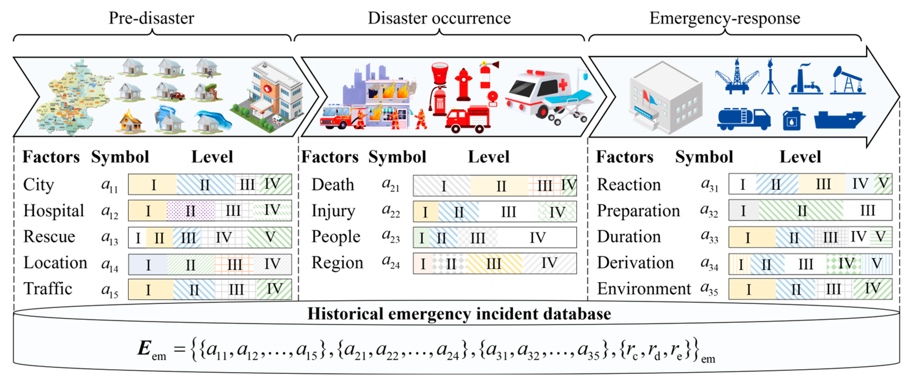
According to the Emergency Response Law of the People’s Republic of China, “emergencies are categorized into four levels based on the post-disaster statistical losses, namely, extremely severe (I), severe (II), significant (III), and general (IV).” Different authorities will implement disposal measures accordingly. Nevertheless, it is impractical to calculate the induced losses or casualties in the post-earthquake emergency response stage. This will hinder real-time relief efforts to these events. To address that, abundant historical emergency events were investigated, and collected into a database. As illustrated in Figure 5, the factors that may have an impact on the entire emergency response process are classified into three groups: pre-disaster, disaster occurrence, and emergency response. Since urgency demands immediate action, limiting the availability of extensive data, these factors are quantified based on types or levels rather than detailed values, as follows:

Figure 5.
Influencing factors and historical emergency incident dataset.
- (1)
- Pre disaster: city level (city level of the disaster site, where I~IV represent first-tier cities, second-tier cities, third-tier cities, and other cities, respectively); distance from the hospital (distance between the disaster site and the nearest hospital, where I~IV represent >10 km, 5~10 km, 2~5 km, and 0~2 km, respectively); distance from rescue agencies (distance between the accident site and the nearest rescue department, where I~IV represent >10 km, 5~10 km, 2~5 km, and 0~2 km, respectively); attributes of the location (category of disaster location, I~V represent commercial/industrial areas, cultural and educational/residential areas, warehousing or development areas, comprehensive areas, and others, respectively); local road network density (road density at the location of the accident, where I~IV represent >6 km/km2, 5~6 km/km2, 4~5 km/km2, and <4 km/km2, respectively).
- (2)
- Disaster occurrence: death toll (number of casualties directly caused by disasters in the first time, I~IV represent ≤3, 4~10, 10~30, and >30, respectively); number of injured individuals (number of injured/trapped people in the first instance of a disaster, I~IV represent <10, 10~50, 50~100, >100, respectively); number of people affected by the disaster (number of people affected by disasters, I~IV represent >105, 104~105, 103~104, <103, respectively); scope of impact (impact scope of the accident, I~IV respectively represent the entire city, a region/CBD, a community/park/multiple main roads, a building/a road, respectively).
- (3)
- Emergency response: emergency response time (time elapsed from the occurrence of a disaster to the initiation of emergency rescue measures, where I~V represent within 3 min, 3~15 min, 15~30 min, 30 min~2 h, and >2 h, respectively); reserved material (reserved materials for responding to sudden disasters, where I~III represent “far exceeding demand”, “basically met”, and “lacking”); duration time (expected duration time from the commencement to the conclusion of emergency measures, where I~V represent within 30 min, 30 min~4 h, 4 h~12 h, 12 h~24 h, and >24 h, respectively); accident evolution (occurrence probability of derivative/secondary hazardous accidents, where I~V represent <0.1%, 0.1%~1%, 1%~10%, 10%~20%, and 20%~50%, respectively); environment condition (weather or driving conditions, I~IV represent good, average, poor, and severe, respectively).
In addition, it is necessary to collect post-disaster statistical results: (number of injuries), (number of deaths), and (economic losses), in order to determine the emergency level (EL) of the disaster. Based on the above analysis, containing 63 emergency events, including the “6.21 Yinchuan Barbecue Shop Explosion”, “4.18 Beijing Changfeng Hospital Fire”, and “8.31 Shanghai Liquid Ammonia Leakage”, have been collected. Due to space limitations, the established databases were uploaded at the website (https://github.com/liuzhenliangstd/EmergencyEventCollection 1 June 2024). And more information can be found by referring to the source website (https://www.ccdi.gov.cn/, accessed on 1 June 2024).
4.2. Decision Tree Based Traffic Demand Generation
The primary purpose of an HBN is to fulfill transportation demands. such as the circulation of personnel and materials among regions. This means meeting the traffic demand (vi and vj are region nodes). Therefore, the specific emergency response measures and means are out of the investigated scope herein. This study explores the feasibility of utilizing a DT methodology to assess the emergency level. By employing this approach, the relevant authorities can be identified, as well as the potential increase in traffic demand (traffic attraction and generation ).
The analysis of the emergency level of sudden disasters is essentially a classification problem. The DT algorithm was applied to learn from the emergency event database data. DT is a non-parametric machine learning algorithm similar to tree decision making (consisting of a root node, several internal nodes, and leaf nodes), with strong interpretability and insensitivity to outliers. 50 and 13 of the emergency data were first randomly divided for training and testing, respectively. Each observation consists of a vector x of inputs (the influencing factors) and an output y (emergency level), as follows:
where and represent the predicted emergency level and actual level of the event, respectively.
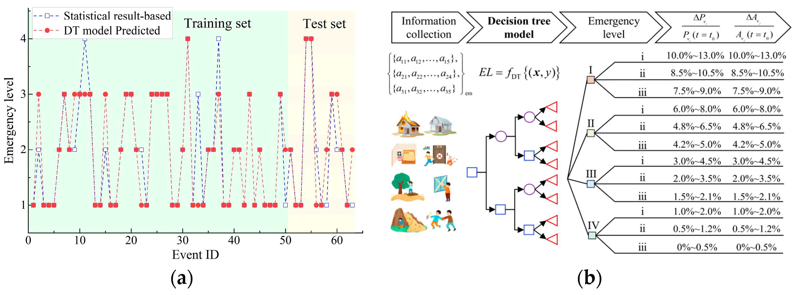
Training a DT model to predict the emergency level is a classification problem. It begins with creating a root node Droot. Subsequently, the training data are grouped based on the Gini coefficient and trained to form a root node. And by gradually segmenting the dataset, a series of internal nodes output binary classification results, up to the leaf nodes, to obtain . Corresponding to the prediction, the cost function is used to measure the error. The change in prediction error due to the split is measured by assessing the reduction in cost achieved by splitting the root node. As shown in Figure 6a, the established DT model quickly and accurately identifies the emergency level of the events. The predicted results of the 42 events of the 50 ones in the training set and 4 events in the test set are consistent with the actual results, with an accuracy rate of about 80%. The inconsistencies in predictions may be attributed to variability in rescue efforts, data limitations, unpredictable random factors such as weather conditions, human errors, model simplification, and the dynamic nature of the emergencies. To address these issues, more detailed rescue data of high accuracy and quality are required to enhance the model’s capabilities. Additionally, implementing models that continuously learn and adapt to real-time updated data and situations can capture the emergencies better. Despite these limitations, the developed DT model can still provide a reasonable evaluation of the level of disaster accidents at the first moment of a disaster.
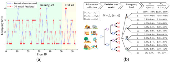
Figure 6.
DT based model for emergency response simulation of HBNs. (a) DT model result comparison. (b) Flowchart and methodologies.
In addition, the specific allocation plan varies depending on the needs and situations of different regions and institutions. The response speed of emergencies is divided into three categories: i (fast), ii (fast), and iii (general), which will lead to varying degrees of traffic generation increase and attraction increase . Consequently, based on pre-earthquake traffic generation and attraction , as well as the speed of rescue work in each region, the post-earthquake traffic demand of the HBN can be adjusted. As illustrated in Figure 6b, post-earthquake traffic demand typically increases due to emergency responses, evacuation needs, and recovery operations, which is a realistic assumption reflecting real-world scenarios. The traffic demand increment depends on the severity of the emergency level, with higher levels indicating more critical situations requiring greater traffic flow. This relationship shows that traffic demand surges from baseline pre-earthquake levels to peak demand at the highest emergency levels. While the figure provides a reasonable assumption of this increment, actual traffic demand levels are typically specified by stakeholders based on local conditions and specific emergency plans. This understanding is crucial for effective resource allocation, emergency response planning, and ensuring infrastructure resilience to manage increased traffic demand during and after an earthquake.
4.3. HBN Emergency Response Model
The pre-disaster traffic demand can be evaluated according to the transportation gravity model, (where and represent traffic generation and attraction, respectively; and are equilibrium coefficients; is the traffic impedance coefficient between vi and vj). For simplicity, the following assumptions are utilized regarding the post-disaster emergency response scenarios:
- (1)
- Inventory information access: the decision-making department can acquire inventory information of emergency material points, meaning the relevant authorities have comprehensive data on available emergency supplies and resources.
- (2)
- Emergency report: responsible persons in each region can promptly report information as per the actual situation; this suggests that there is efficient communication and reporting mechanisms in place to relay information about the emergency status.
- (3)
- Emergency response in HBNs: the focus of the emergency response scenario is solely on traffic-related aspects that depend on the Highway Bridge Network (HBN) transportation; other aspects such as material transportation decrease, and social organization capacity are not considered in this scenario.
- (4)
- Material allocation: material allocation decisions prioritize fairness (maximizing demand rate) and efficiency (minimizing time), rather than economy and environmental protection, etc.
- (5)
- Travel path selection: all vehicles opt for the shortest available path on the primary transportation routes provided by the HBN.
These assumptions help define the scope and context of the emergency response scenario, providing clarity on the factors considered and the limitations of the model. Based on these factors, the post-earthquake emergency response within an HBN can be simulated.
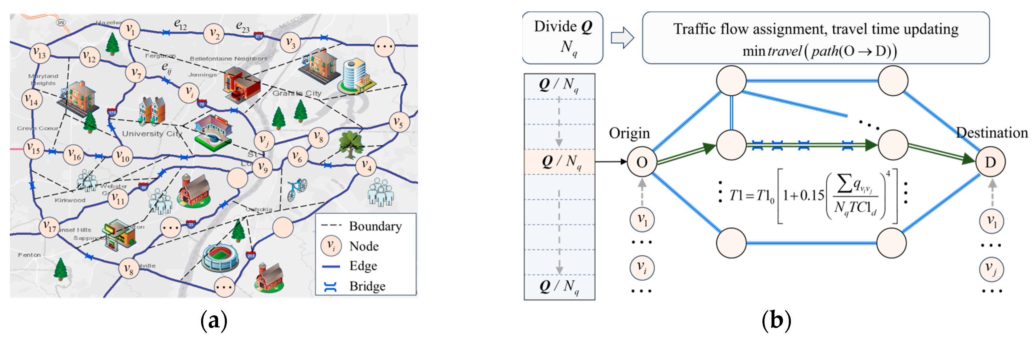
As shown in Figure 7a, for a hypothetical area connected by an HBN, the research area can be divided into several sub-areas according to the administrative division criteria. Each one is represented by a node vi. Then the area can be formed into a node set V = {vi}. Additionally, the main road connecting region vi and vj is represented by the connecting edge eij. All of the road segments can be formed into an edge set E = {eij}. A graph model G = {V, E} of the HBN can be established. The weights of the edges are the traffic capacity TC(eij) and time Tt(eij), which will be updated in the recovery process according to Equation (4). Subsequently, for each node vi, as the starting point (O) and destination point (D), the incremental traffic allocation method is used to select the minimum travel time route for the traffic demand between each OD set, as shown in Figure 7b. The OD traffic demand is divided into Nq subsets, each of which will be assigned to the fastest path step by step. Each subset represents a fraction of the total traffic demand among OD. During that process, the travel time of the roads will be continuously updated according to Equation (5), such as to account for the additional traffic time caused by the newly assigned traffic load. By continuously updating the travel times, the model ensures that each subsequent subset of traffic is routed based on the most current conditions, thereby optimizing the overall traffic distribution across the network. The travel time T1(eij) of the link eij can be updated based on traffic flow and capacity ( and are the number of lanes and capacity per lane, respectively).
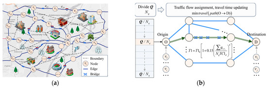
Figure 7.
Schematic of post-earthquake emergency response simulation of HBN. (a) Illustration of nodes and connection edges. (b) Traffic flow simulation.
Finally, the travel time and operational status of HBNs can be simulated, such as to evaluate their functionalities as follows:
5. Emergency Response Resilience Assessment
5.1. Time-Variant Functionality of HBN
The evolving recovery process of functionalities over time is crucial in seismic resilience assessment. During the post-earthquake emergency rescue phase, the functions undertaken by HBNs are diverse, a single resilience indicator is difficult to comprehensively consider the various emergency functions. They are divided into five parts: (1) rescue of injured persons F1; (2) transfer of affected personnel and implementation of preventive measures F2; (3) emergency repair, restoration, or demolition of damaged buildings and facilities F3; (4) allocation and transportation of rescue materials F4; (5) ensuring other activities or travel F5.
Current resilience investigations of HBNs predominantly utilize indirect metrics like travel time or distance [44]. These metrics provide valuable insights, yet they also have limitations. For instance, they may not capture the variations in the dynamic nature of post-seismic recovery. Moreover, these indirect indicators may overlook the availability of alternate routes or traffic demand satisfactions. To address these limitations, is proposed to represent the ability of the HBN meeting the traffic demand as the emergency function Fk at time t. It can be quantified by the ratio of materials that can be obtained on time to the demand, as follows:
where and represent the capacity and demand of the emergency function Fk between time vi and vj at time t after the earthquake, that is, the traffic volume that can and needs to meet per hour.
5.2. Cumulative Resilience Vector
Seismic emergency resilience refers to the system’s capacity to withstand or rapidly return to a predefined functional level during emergency situations following an earthquake. This includes the immediate emergency response phase and excludes subsequent recovery and reconstruction phases, as illustrated in Figure 8. In response to the current lack of research, this article proposes a multidimensional seismic emergency resilience evaluation index vector to comprehensively measure the seismic emergency resilience of HBNs. According to Bruneau et al. [45], the resilience index can be calculated based on the average value of the system function F(t) from the time of earthquake occurrence t0 to the time of recovery completion t0 + th, as shown below:
where th is the recovery duration of the HBN. It should be noted that the duration of emergency response is not solely determined by the time required to restore HBN functionality to its pre-earthquake state. Instead, it is contingent upon meeting emergency requirements and ensuring the safety and well-being of affected individuals and communities.
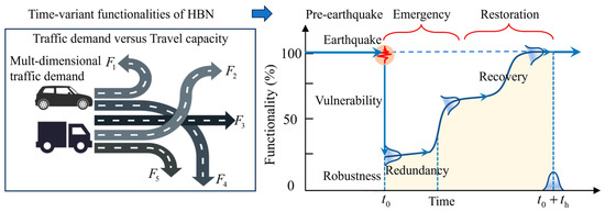
Figure 8.
Seismic emergency resilience illustration of HBN.
By directly measuring the extent to which bridges meet functional requirements following a seismic event, this method offers a more comprehensive understanding of HBNs’ functionality. It enables policymakers and engineers to make informed decisions regarding infrastructure investments and emergency response planning, ultimately enhancing the overall resilience of bridge networks in seismic-prone regions.
6. Application to HBN Case Studies
6.1. Regional Seismic Hazard and Bridge Damage State
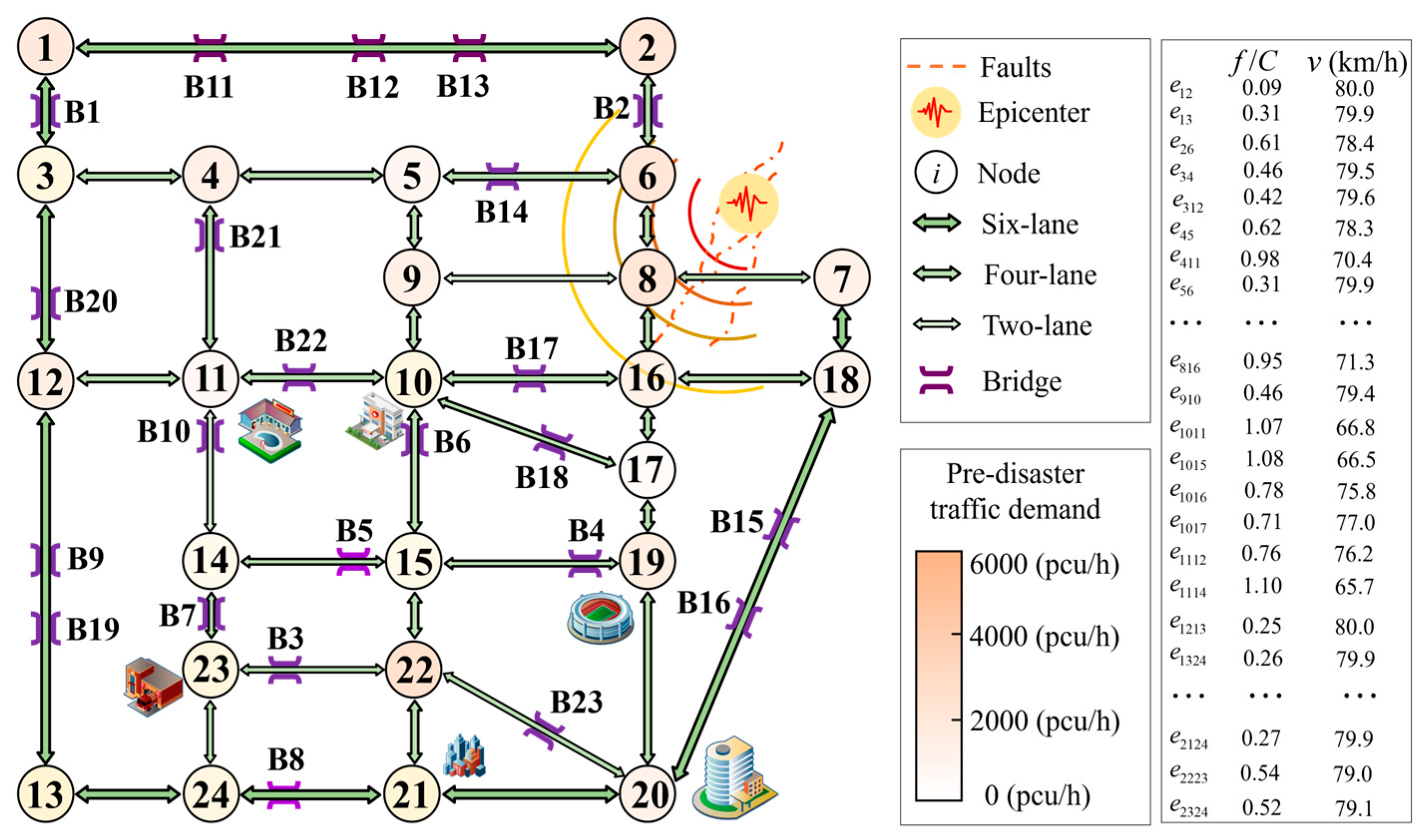
The seismic emergency resilience of the Sioux Falls network is analyzed to verify the proposed methodologies. This HBN includes a variety of road types and intersections. To align with its scale and complexity, its location is assumed to be a second-tier city. Second-tier cities usually have a population and traffic volume that is significant but not overwhelming, enabling detailed analysis without the computational intensity required for larger metropolitan areas. As shown in Figure 9, the HBN connects 24 regions through 38 highway segments. The network is composed of various types of regions as follows:
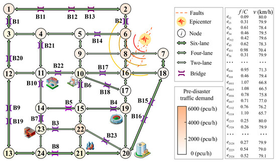
Figure 9.
Schematic layout of the HBN for post-earthquake simulation.
- (1)
- Nodes 1, 2, 3, 7, 8, 12, and 18 are industrial areas;
- (2)
- Nodes 4, 5, 6, 9, 14, and 16 are commercial areas;
- (3)
- Nodes 13, 21, and 24 are storage/development areas;
- (4)
- Nodes 15, 17, 20, and 22 are comprehensive areas;
- (5)
- Nodes 11 and 19 are schools and sports fields (used as emergency evacuation points in emergency stages);
- (6)
- Node 10 is the location of the hospital;
- (7)
- Node 23 is the location of the fire brigade.
The pre-earthquake traffic generation and traffic attraction of each regional node range from 1280 pcu/h to 5740 pcu/h. To reflect the diversity of road segment characteristics in the bridge network, appropriate adjustments have been made to the basic road features. The number of lanes is 2–6, the width is 3.75 m per lane, the basic free flow capacity is 2200 pcu/h, and the free-flow speed is 80 km/h. Based on this, the HBN node set V, connection matrix E, traffic demand Q among different regions, traffic capacity TCB of each section, and maximum traffic speed TSB can be determined. By combining the network topology structure, the functionalities of the HBN can be simulated using the previous method. As can be seen, the majority of the highway sections had a congestion rate smaller than 1.0 and an average speed of larger than 75 km/h before the earthquake. All of the traffic demands can be met.
In addition, the HBN includes 23 bridges with a designed service life of 100 years, currently ranging in age from 10 to 60 years, as illustrated in Table 3. This analysis does not account for the impact of maintenance measures on each bridge during its service life. The atmospheric chloride ion concentration and chloride ion diffusion coefficient in the service area are 2.95 kg/m3 and 129 mm2/year, respectively. The site category in this area is Class B, with an average shear wave velocity of 450 m/s within 30 m, mainly threatened by the northeast reverse fault in the area. This study simplifies it as an earthquake caused by seismic motion at the epicenter of the region, with an average rupture angle of 75° and a depth of 10 km. The Richter scale is 7.0 (Mw = 7.0).
Table 3.
Basic characteristics of the regional bridges.
6.2. Seismic Damage Distribution of Regional Bridges
According to the seismic source characteristics, the potential seismic sources can be identified. The likelihood of seismic motion intensities is then quantified using the Probability Seismic Hazard Analysis (PSHA) method. The distance from the epicenter to each bridge site is calculated to reflect the seismic wave amplitude propagation. Subsequently, the Ground Motion Prediction Equation (GMPE) is used to estimate the expected IM at each bridge location under seismic motion. Combining the contributions from all seismic sources, the probability of exceeding various levels of IM at each bridge site can be estimated. Given the necessity for a micro-level analysis of the seismic performance of regional bridges, this paper chooses the GMPE model proposed by Kumar et al. [46]. This model is based on a large number of shallow seismic records, with good fitting results, and is suitable for the area where the bridge network is located, as shown below:
where Mw is the magnitude, RJB is the epicenter distance, and is the total standard deviation of the prediction model, taken as 0.281. In order to consider the uncertainty of seismic motion, 103 sets of seismic motion Sa values were generated through MCS to simulate earthquake scenarios for regional bridge seismic damage analysis.
To obtain the evolution process of the seismic emergency resilience of the HBN during its service life, the earthquake occurrence time t0 is taken as five time points: 0 years, 10 years, 20 years, 30 years, and 40 years later. For each time point, the time-varying performance of each bridge during its service life is determined based on the performance degradation model. This article mainly considers the mechanical attenuation mechanism of bridge pier columns caused by environmental corrosion. According to the degradation mechanisms proposed by Ghosh et al. [47], the model parameters of bridges can be updated. In this model, when chloride ions permeate the concrete cover, namely t > Tini, the steel bars start to corrode, leading to a decreasing longitudinal reinforcement ratio . This approach enables the prediction of the evolving seismic fragilities of the bridges, highlighting the impact of long-term environmental exposure on their structural performance.
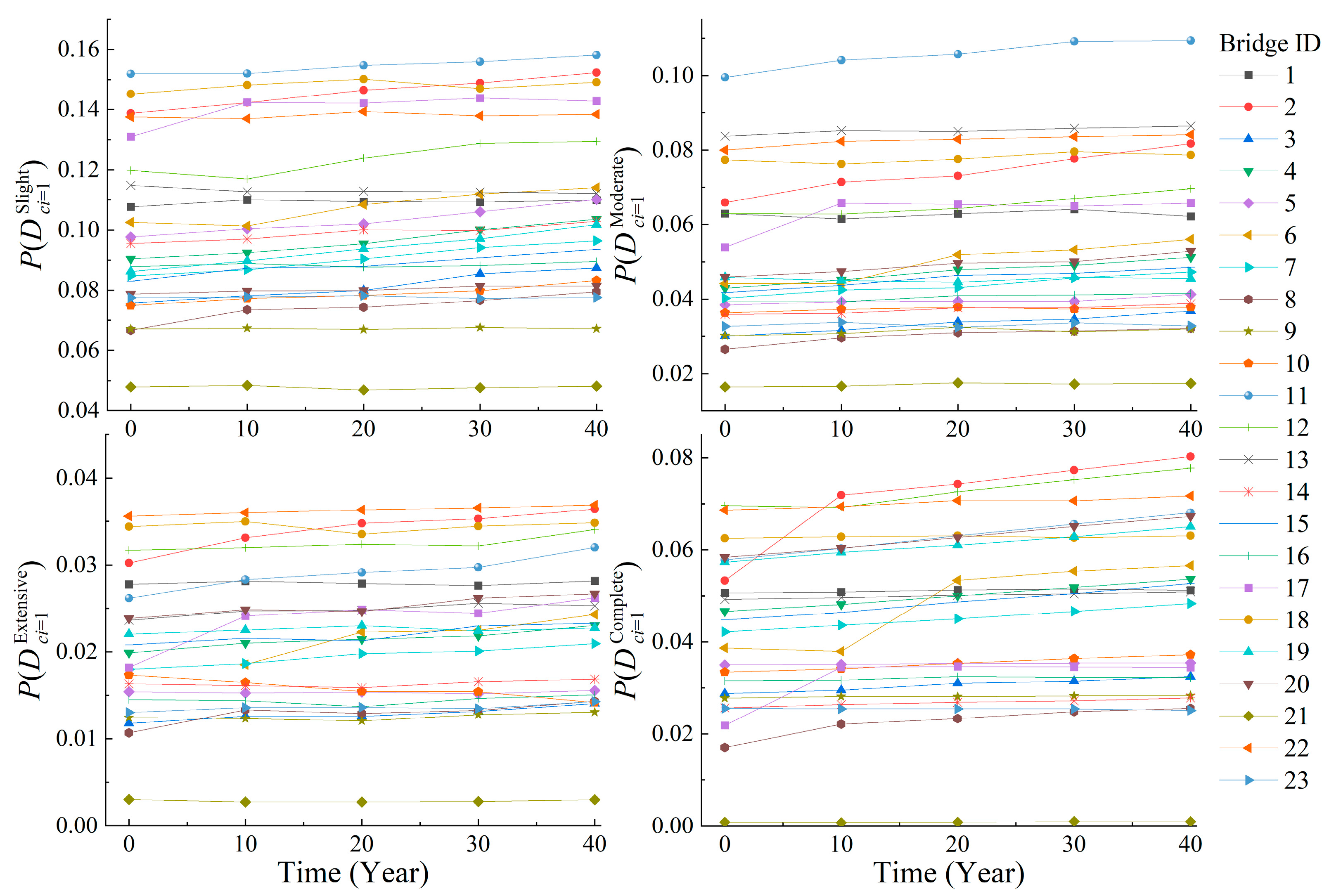
In order to account for the inherent uncertainties, MCS is used to sample each bridge and simulate the degradation process of each bridge’s characteristics, thereby establishing 103 bridge samples. Combined with seismic intensity samples, 106 bridge seismic samples were obtained. This process requires creating finite element models and conducting extensive seismic time history analyses using the conventional IDA method, rendering long-term seismic performance analysis of regional bridges nearly impractical. Alternatively, the established ANN model for seismic analysis was then used to predict the seismic damage states and probability of key components of regional bridges in the HBN. The figures in Figure 10 depict the time-varying seismic damage probabilities of bridge piers. It can be observed that environmental corrosion increases the probability of damage to bridges. For example, during the 0–40 year service life, the probabilities of slight and severe damage to the piers of bridge B1 action increased from 0.105 and 0.027 to 0.110 and 0.028, respectively, while the probabilities of slight and severe damage to the piers of bridge B6 increase from 0.102 and 0.017 to 0.114 and 0.024, respectively. Notably, there is a decrease observed in the probability of certain damage levels in some cases, such as the probabilities of B5 and B8 in moderate damage state. This can be attributed to changes in specific structural characteristics of the bridge over its service life. For example, corrosion-induced degradation will lead to a decrease in the reinforcement ratio of bridge piers, which can significantly affect the bridge’s response to seismic excitations. If the bridge’s response undergoes a sharp increase, surpassing the limit states for moderate damage, and tends to increase dramatically, exceeding the limit states of moderate damage, the probabilities of moderate state will decrease. However, this may cause the bridge to experience severe or complete damage, leading to an increase in the probabilities of extensive or complete damage. In summary, the developed ANN surrogates can capture complex effects of various factors, providing the evolving seismic behaviors of bridges.
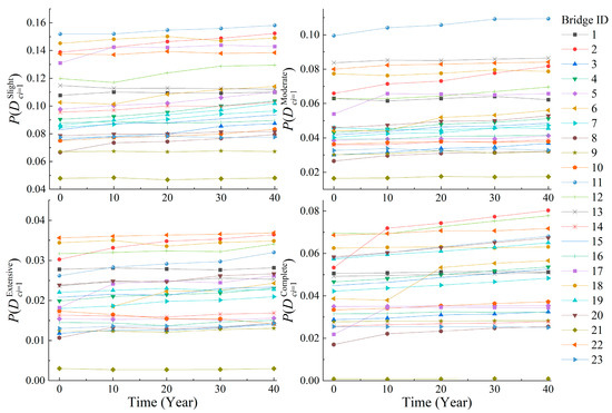
Figure 10.
Seismic damage evolution of the piers of regional bridges.
Based on the damage to key components of bridges and the resulting traffic restrictions, the traffic capacity of the highway segment where the bridge is located can be evaluated. This helps determine the process of restoring the traffic function of the damaged bridge.
6.3. Seismic Emergency Resilience during Service Life
Using the previous methods, the post-earthquake emergency level and functionality recovery process of the HBN were investigated. And the satisfaction of different traffic emergency needs under earthquake action at different time points was analyzed. The seismic emergency resilience of the HBN was obtained, which took about 107 min (with an average simulation time of about 0.07 s). It can be seen that the intelligent analysis model can achieve rapid evaluation of seismic resilience of HBNs, which is crucial for timely and effective emergency response and recovery planning.
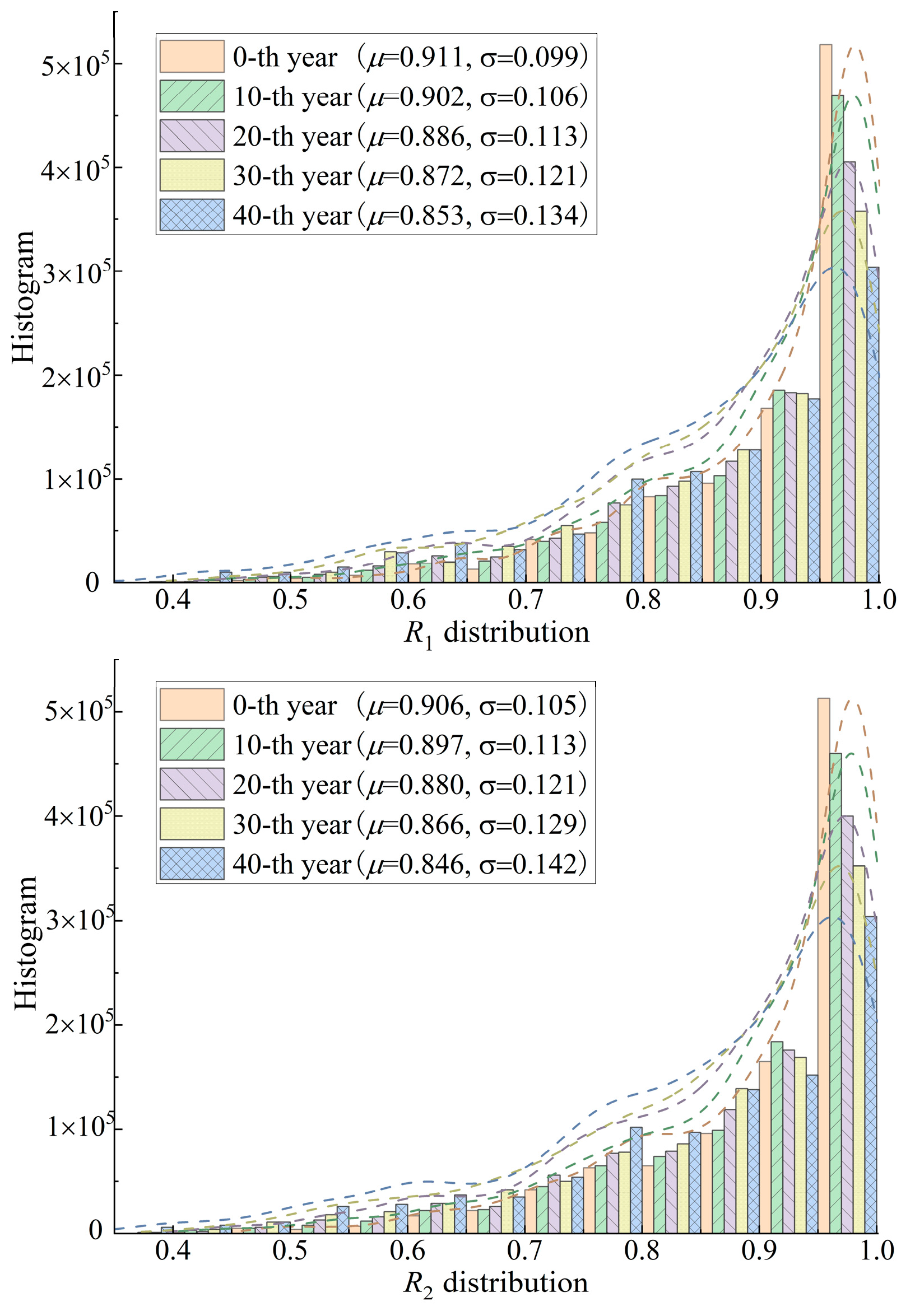
Figure 11 shows the analysis results and distribution of emergency resilience indicators R1 and R2 of the HBN, which predominantly range between 0.68 and 1.0. It can be seen that under the assumed earthquake scenario, the HBN is highly likely to meet the traffic demand, with a 67.8% probability of R1 exceeding 0.9 at the current stage. However, special attention should still be paid to some special situations, such as when bridge B1 and B11 are completely destroyed simultaneously. This will cause zone 1 (node 1 in the HBN) to be isolated from other areas, reducing the resilience value to less than 0.5, and greatly hindering seismic rescue efforts. This highlights the need to prioritize the maintenance and retrofitting of critical bridges, such as B1 and B11, whose failure would severely disrupt network connectivity. Ensuring these key structures are resilient can prevent the isolation of critical zones.
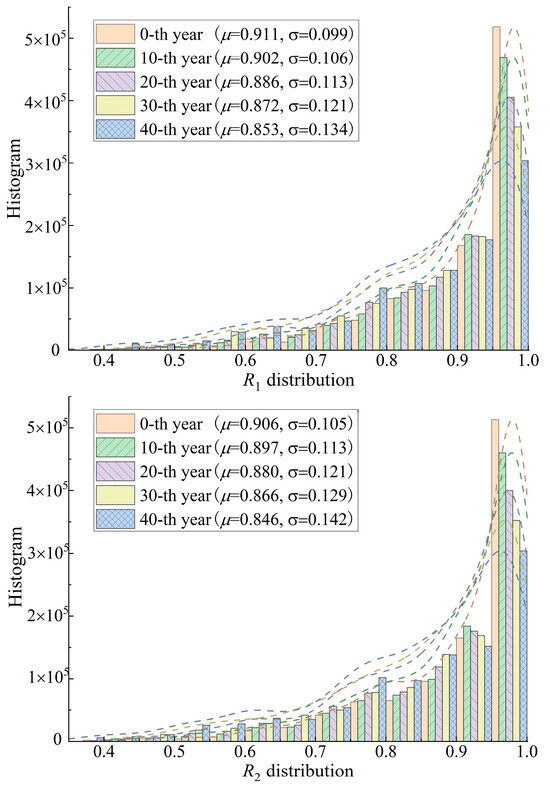
Figure 11.
Seismic emergency resilience of the bridge network in service period.
In addition, for overextended service periods, the emergency performance of the HBN will deteriorate, and the discreteness will gradually increase. For example, R1 mean μ decreases from 0.911 to 0.853, while standard deviation σ increases from 0.099 to 0.134. This is because during long-term service, the degradation process and mechanical performance of different bridges have significant discreteness, which has an increasing impact on the seismic performance of bridges, leading to an increase in the discreteness of toughness analysis. The degradation patterns of different seismic emergency resilience indicators also differ. Notably, the mean (μ) and standard deviation (σ) of R2 changed from 0.906 to 0.846 and from 0.105 to 0.142, respectively. The results suggest the need for long-term planning and investment in bridge maintenance. Incorporating resilience criteria into these standards can ensure that future infrastructure is better equipped to withstand seismic events. Therefore, regular inspections and upgrades should be scheduled to address the gradual degradation of bridge performance and ensure sustained resilience over time.
Overall, the intelligent evaluation method established in this article can quickly and accurately assess the seismic emergency resilience of HBNs throughout their service life. In practical engineering applications, this method allows for the analysis of emergency resilience under various seismic conditions (such as magnitude, site, epicenter distance, and source depth) and service environments. It comprehensively deduces the process of emergency resilience changes and studies the impact of different emergency strategies on resilience. This approach provides a robust decision-making basis for formulating emergency plans and strategies for disaster prevention and mitigation.
7. Conclusions
This article presents a holistic framework for the seismic emergency response of HBNs. It comprehensively integrates the influencing factors like seismic hazards, bridge vulnerabilities, and traffic capacity. The emergency response resilience is quantified in terms of its rescue, evacuation, and other metrics. The following conclusions can be drawn:
- (1)
- The ANN-based analysis method proposed in this article can substitute for the IDA-based method to efficiently evaluate the time-varying seismic performance of regional bridges.
- (2)
- The DT model driven by historical emergency response cases has shown considerable potential in emergency simulation, providing strong support for emergency decision making in HBNs.
- (3)
- The established HBN seismic emergency resilience assessment system comprehensively considers the dynamic changes in emergency material allocation, evacuation, and rescue operations.
The proposed methodologies can be implemented to support decision making for emergency response, emergency planning, and other related activities. However, this study has several limitations: (1) it primarily focuses on post-disaster scenarios such as centralized rescue and evacuation, neglecting the roles of temporary emergency forces organized by society and the passive cancellation of travel; (2) bridges were assumed to be the only vulnerable elements in an HBN, whereas in reality, other seismic-induced losses like highway damages and debris will also impede the emergency response. Future research should further explore the comprehensive factors and impacts of various transportation needs and emergency response technologies.
Author Contributions
Conceptualization and methodology, L.M.; software, C.Z. and Z.L.; validation, K.F. and X.L.; formal analysis, C.Z.; writing—original draft preparation, Z.L.; writing—review and editing, L.M.; visualization, Z.L.; supervision, L.M.; funding acquisition, Z.L. All authors have read and agreed to the published version of the manuscript.
Funding
This research was funded by the National Natural Science Foundation of China, grant number 52308512, Hebei Natural Science Foundation of China, grant number E2022210048, and 2024 Outstanding Youth Science Fund Project of Shijiazhuang Tiedao University.
Institutional Review Board Statement
Not applicable.
Informed Consent Statement
Not applicable.
Data Availability Statement
All data, models, and codes supporting the findings of this study are available from the corresponding author upon reasonable request.
Conflicts of Interest
The authors declare no conflict of interest.
References
- Liu, H.; He, Y. Comprehensive Evaluation of Resilience for Qinling Tunnel Group Operation Safety System Based on Combined Weighting and Cloud Model. Sustainability 2024, 16, 3937. [Google Scholar] [CrossRef]
- Mitoulis, S.A.; Argyroudis, S.A.; Loli, M.; Imam, B. Restoration models for quantifying flood resilience of bridges. Eng. Struct. 2021, 238, 112180. [Google Scholar] [CrossRef]
- Zhu, S. Is the 2013 Lushan earthquake (Mw = 6.6) a strong aftershock of the 2008 Wenchuan, China mainshock (Mw = 7.9)? J. Geodyn. 2016, 99, 16–26. [Google Scholar] [CrossRef]
- Zhu, M.; Li, J.; Zhao, F.; Xu, Y.; Li, W. Analysis of highway damage characteristics from 2022 Luding Ms6.8 earthquake. World Earthq. Eng. 2024, 40, 197–207. [Google Scholar]
- Zhang, K.; Lee, J.E. Assessing the Operational Capability of Disaster and Emergency Management Resources: Using Analytic Hierarchy Process. Sustainability 2024, 16, 3933. [Google Scholar] [CrossRef]
- Choi, S.; Chae, J.; Do, M. Emergency Road Network Determination for Seoul Metropolitan Area. Sustainability 2022, 14, 5422. [Google Scholar] [CrossRef]
- Moschonas, I.F.; Kappos, A.J.; Panetsos, P.; Papadopoulos, V.; Makarios, T.; Thanopoulos, P. Seismic fragility curves for greek bridges: Methodology and case studies. Bull. Earthq. Eng. 2009, 7, 439–468. [Google Scholar] [CrossRef]
- Mangalathu, S.; Jeon, J.-S.; Padgett, J.E.; DesRoches, R. Performance-based grouping methods of bridge classes for regional seismic risk assessment: Application of ANOVA, ANCOVA, and non-parametric approaches. Earthq. Eng. Struct. Dyn. 2017, 46, 2587–2602. [Google Scholar] [CrossRef]
- Zentner, I.; Gündel, M.; Bonfils, N. Fragility analysis methods: Review of existing approaches and application. Nucl. Eng. Des. 2016, 323, 245–258. [Google Scholar] [CrossRef]
- Li, S.; Li, S.; Laima, S.; Li, H. Data-driven modeling of bridge buffeting in the time domain using long short-term memory network based on structural health monitoring. Struct. Contr. Health Monit. 2021, 28, e2772. [Google Scholar] [CrossRef]
- Liu, Z.; Li, S.; Guo, A.; Li, H. Comprehensive functional resilience assessment methodology for bridge networks using data-driven fragility models. Soil Dyn. Earthq. Eng. 2022, 159, 107326. [Google Scholar] [CrossRef]
- Abbiati, G.; Broccardo, M.; Abdallah, I.; Marelli, S.; Paolacci, F. Seismic fragility analysis based on artificial ground motions and surrogate modeling of validated structural simulators. Earthq. Eng. Struct. Dyn. 2021, 50, 2314–2333. [Google Scholar] [CrossRef]
- Fan, G.; Li, J.; Hao, H.; Xin, Y. Data driven structural dynamic response reconstruction using segment based generative adversarial networks. Eng. Struct. 2021, 234, 111970. [Google Scholar] [CrossRef]
- Mangalathu, S.; Hwang, S.-H.; Choi, E.; Jeon, J.-S. Rapid seismic damage evaluation of bridge portfolios using machine learning techniques. Eng. Struct. 2019, 201, 109785. [Google Scholar] [CrossRef]
- Tavares, D.H.; Padgett, J.E.; Paultre, P. Fragility curves of typical as-built highway bridges in eastern Canada. Eng. Struct. 2012, 40, 107–118. [Google Scholar] [CrossRef]
- Xu, H.; Gardoni, P. Probabilistic capacity and seismic demand models and fragility estimates for reinforced concrete buildings based on three-dimensional analyses. Eng. Struct. 2016, 112, 200–214. [Google Scholar] [CrossRef]
- Liu, Z.; Sextos, A.; Guo, A.; Zhao, W. ANN-based rapid seismic fragility analysis for multi-span concrete bridges. Structures 2022, 41, 804–817. [Google Scholar] [CrossRef]
- Rajkumari, S.; Thakkar, K.; Goyal, H. Fragility analysis of structures subjected to seismic excitation: A state-of-the-art review. Structures 2022, 40, 303–316. [Google Scholar] [CrossRef]
- Li, B.; Chuang, W.-C.; Spence Seymour, M.J. Response Estimation of Multi-Degree-of-Freedom Nonlinear Stochastic Structural Systems through Metamodeling. J. Eng. Mech. 2021, 147, 04021082. [Google Scholar] [CrossRef]
- Gu, Y.; Lu, X.; Xu, Y. A deep ensemble learning-driven method for the intelligent construction of structural hysteresis models. Comput. Struct. 2023, 286, 107106. [Google Scholar] [CrossRef]
- Xu, J.-G.; Feng, D.-C.; Mangalathu, S.; Jeon, J.-S. Data-driven rapid damage evaluation for life-cycle seismic assessment of regional reinforced concrete bridges. Earthq. Eng. Struct. Dyn. 2022, 51, 2730–2751. [Google Scholar] [CrossRef]
- Kameshwar, S.; Misra, S.; Padgett, J.E. Decision tree based bridge restoration models for extreme event performance assessment of regional road networks. Struct. Infrastruct. Eng. 2019, 3, 431–451. [Google Scholar] [CrossRef]
- Edrissi, A.; Nourinejad, M.; Roorda, M.J. Transportation network reliability in emergency response. Transp. Res. Part E Logist. Transp. Rev. 2015, 80, 56–73. [Google Scholar] [CrossRef]
- Chen, M.; Mangalathu, S.; Jeon, J.-S. Bridge fragilities to network fragilities in seismic scenarios: An integrated approach. Eng. Struct. 2021, 237, 112212. [Google Scholar] [CrossRef]
- Shen, Z.; Liu, Y.; Liu, J.; Liu, Z.; Han, S.; Lan, S. A Decision-Making Method for Bridge Network Maintenance Based on Disease Transmission and NSGA-II. Sustainability 2023, 15, 5007. [Google Scholar] [CrossRef]
- Hosseini, S.; Barker, K.; Ramirez-Marquez, J.E. A review of definitions and measures of system resilience. Reliab. Eng. Syst. Saf. 2016, 145, 47–61. [Google Scholar] [CrossRef]
- Romero-Lankao, P.; Gnatz, D.M.; Wilhelmi, O.; Hayden, M. Urban Sustainability and Resilience: From Theory to Practice. Sustainability 2016, 8, 1224. [Google Scholar] [CrossRef]
- Hosseini, Y.; Karami Mohammadi, R.; Yang, T.Y. Resource-based seismic resilience optimization of the blocked urban road network in emergency response phase considering uncertainties. Int. J. Disaster Risk Reduct. 2023, 85, 103496. [Google Scholar] [CrossRef]
- Kiremidjian, A.; Moore, J.; Fan, Y.Y.; Yazlali, O.; Basoz, N.; Williams, M. Seismic Risk Assessment of Transportation Network Systems. J. Earthq. Eng. 2007, 11, 371–382. [Google Scholar] [CrossRef]
- Xiong, C.; Huang, J.; Lu, X. Framework for city-scale building seismic resilience simulation and repair scheduling with labor constraints driven by time–history analysis. Comput.-Aided Civ. Infrastruct. Eng. 2019, 35, 322–341. [Google Scholar] [CrossRef]
- Kim, S.; Ge, B.; Frangopol Dan, M. Optimum Target Reliability Determination for Efficient Service Life Management of Bridge Networks. J. Bridge Eng. 2020, 25, 04020087. [Google Scholar] [CrossRef]
- Li, Y.; Dong, Y.; Frangopol, D.M.; Gautam, D. Long-term resilience and loss assessment of highway bridges under multiple natural hazards. Struct. Infrastruct. Eng. 2020, 16, 626–641. [Google Scholar] [CrossRef]
- Nielson, B.G.; Desroches, R. Seismic fragility methodology for highway bridges using a component level approach. Earthq. Eng. Struct. Dyn. 2007, 36, 823–839. [Google Scholar] [CrossRef]
- Du, A.; Padgett, J.E. Entropy-based intensity measure selection for site-specific probabilistic seismic risk assessment. Earthq. Eng. Struct. Dyn. 2021, 50, 560–579. [Google Scholar] [CrossRef]
- Mangalathu, S.; Karthikeyan, K.; Feng, D.-C.; Jeon, J.-S. Machine-learning interpretability techniques for seismic performance assessment of infrastructure systems. Eng. Struct. 2022, 250, 112883. [Google Scholar] [CrossRef]
- Shamsabadi, A.; Khalili-Tehrani, P.; Stewart Jonathan, P.; Taciroglu, E. Validated Simulation Models for Lateral Response of Bridge Abutments with Typical Backfills. J. Bridge Eng. 2010, 15, 302–311. [Google Scholar] [CrossRef]
- Du, A.; Padgett, J.E. Toward confident regional seismic risk assessment of spatially distributed structural portfolios via entropy-based intensity measure selection. Bull. Earthq. Eng. 2020, 18, 6283–6311. [Google Scholar] [CrossRef]
- Pang, Y.; Wei, K.; Yuan, W. Life-cycle seismic resilience assessment of highway bridges with fiber-reinforced concrete piers in the corrosive environment. Eng. Struct. 2020, 222, 111120. [Google Scholar] [CrossRef]
- Mangalathu, S.; Jeon, J.-S. Stripe-based fragility analysis of multispan concrete bridge classes using machine learning techniques. Earthq. Eng. Struct. Dyn. 2019, 48, 1238–1255. [Google Scholar] [CrossRef]
- Baker, J.; Lin, T.; Shahi, S.; Jayaram, N. New Ground Motion Selection Procedures and Selected Motions for the PEER Transportation Research Program; Pacific Earthquake Engineering Research Center, College of Engineering, University of California: Berkeley, CA, USA; Department of Civil and Environmental Engineering, Stanford University: Stanford, CA, USA, 2011. [Google Scholar]
- McKenna, F. OpenSees: A Framework for Earthquake Engineering Simulation. Comput. Sci. Eng. 2011, 13, 58–66. [Google Scholar] [CrossRef]
- Board, T.R. Highway Capacity Manual 6th Edition: A Guide for Multimodal Mobility Analysis; The National Academies Press: Washington, DC, USA, 2016. [Google Scholar]
- Liu, Z.; Yuan, W.; Li, S. Resilience assessment study of highway bridge networks subjected to both earthquakes and earthquake-induced secondary emergencies. China Saf. Sci. J. 2022, 08, 176–184. [Google Scholar]
- Wu, Y.; Chen, S. Transportation Resilience Modeling and Bridge Reconstruction Planning Based on Time-Evolving Travel Demand during Post-Earthquake Recovery Period. Sustainability 2023, 15, 12751. [Google Scholar] [CrossRef]
- Bruneau, M.; Chang, S.E.; Eguchi, R.T.; Lee, G.C.; O’Rourke, T.D.; Reinhorn, A.M.; Shinozuka, M.; Tierney, K.; Wallace, W.A.; von Winterfeldt, D. A Framework to Quantitatively Assess and Enhance the Seismic Resilience of Communities. Earthq. Spectra 2003, 19, 733–752. [Google Scholar] [CrossRef]
- Kumar, P.; Chamoli, B.P.; Kumar, A.; Gairola, A. Attenuation Relationship for Peak Horizontal Acceleration of Strong Ground Motion of Uttarakhand Region of Central Himalayas. J. Earthq. Eng. 2021, 25, 2537–2554. [Google Scholar] [CrossRef]
- Ghosh, J.; Padgett Jamie, E. Aging Considerations in the Development of Time-Dependent Seismic Fragility Curves. J. Struct. Eng. 2010, 136, 1497–1511. [Google Scholar] [CrossRef]

Disclaimer/Publisher’s Note: The statements, opinions and data contained in all publications are solely those of the individual author(s) and contributor(s) and not of MDPI and/or the editor(s). MDPI and/or the editor(s) disclaim responsibility for any injury to people or property resulting from any ideas, methods, instructions or products referred to in the content. |
© 2024 by the authors. Licensee MDPI, Basel, Switzerland. This article is an open access article distributed under the terms and conditions of the Creative Commons Attribution (CC BY) license (https://creativecommons.org/licenses/by/4.0/).