Abstract
The World Air Quality Index indicates that Pakistan ranks as the third most polluted country, regarding the average (Particulate Matter) PM2.5 concentration, which is 14.2 times higher than the World Health Organization’s annual air quality guideline. It is crucial to implement a program aimed at reducing PM2.5 levels in Pakistan’s urban areas. This review paper highlights the importance of indoor air pollution in urban regions such as Lahore, Faisalabad, Gujranwala, Rawalpindi, and Karachi, while also considering the effects of outdoor air temperature on occupants’ thermal comfort. The study aims to evaluate past methodological approaches to enhance indoor air quality in buildings. The main research question is to address whether there are statistical correlations between the PM2.5 and the operative air temperature and whether other indoor climatic variables have an impact on the thermal comfort assessment in densely built urban agglomeration regions in Pakistan. A systematic review analysis method was employed to investigate the effects of particulate matter (PM2.5), carbon oxides (COx), nitrogen oxides (NOx), sulfur oxides (SOx), and volatile organic compounds (VOCs) on residents’ health. The Preferred Reporting Items for Systematic Reviews and Meta Analyses (PRISMA) protocol guided the identification of key terms and the extraction of cited studies. The literature review incorporated a combination of descriptive research methods to inform the research context regarding both ambient and indoor air quality, providing a theoretical and methodological framework for understanding air pollution and its mitigation in various global contexts. The study found a marginally significant relationship between the PM2.5 operative air temperature and occupants’ overall temperature satisfaction, Ordinal Regression (OR) = 0.958 (95%—Confidence Interval (CI) [0.918, 1.000]), p = 0.050, Nagelkerke − Regression (R2) = 0.042. The study contributes to research on the development of an evidence-based thermal comfort assessment benchmark criteria for the American Society of Heating, Refrigerating and Air-Conditioning Engineers (ASHRAE) Global Thermal Comfort Database version 2.1.
1. Introduction
In the present era, indoor air quality (IAQ) has become a matter of significant concern for nations across the globe. This is primarily due to the substantial amount of time that individuals spend indoors. It is crucial to prioritize and improve the air quality in indoor spaces, as it directly impacts human health. Pakistan faces a critical challenge, as indoor air pollution poses a grave threat to public well-being. According to the World Air Quality Report 2020, several urban regions in Pakistan have gained notoriety for being among the most polluted in the world. This report relies on the assessment of average annual concentrations of fine particulate matter (PM2.5) to determine the severity of air pollution. Tragically, the repercussions of indoor air pollution encompass an increased risk of respiratory and cardiovascular ailments, as well as a heightened susceptibility to cancer [1]. According to a study by the Environmental Protection Agency of Pakistan (EPA), indoor air pollution in Pakistan is four times higher than outdoor air pollution. In addition to this, air pollution is responsible for 22% of Pakistan’s deaths, as the World Health Organization (WHO) reported. Various studies have shown that much of the outdoor PM generated by biomass burning can migrate to the indoor environment via advection (via open windows/doors) or infiltration (via door and window gaps or enclosed structures), resulting in elevated indoor PM concentrations [2,3,4].
Belias and Licina (2024) identified the correlations between residential ventilation systems, indoor air quality (IAQ), and energy demand across nine European cities [5]. The study used both outdoor air pollution and meteorological data with building energy simulations. To accomplish this, the study evaluated the effectiveness of five different ventilation systems and three ventilative cooling (VC) scenarios. The study findings indicated that PM2.5 was the primary contributor to disability-adjusted life years (DALYs), accounting for approximately 94% of the total. It was found that filtering outdoor air reduced DALYs by 37%, while VC based on both indoor and outdoor parameters increased DALYs by between 1.1 and 1.4%. Demand-controlled mechanical ventilation with energy recovery and outdoor air filtration showed strong correlations between health and energy efficiency, although it had a higher energy demand of 17.2% for an 8.6% reduction in DALYs. The study highlighted the importance of integrating both indoor and outdoor environmental factors in designing ventilation systems to optimize indoor air quality and energy use.
Considine et al. (2024) developed and tested an aspiration efficiency reducer (AER) to improve energy efficiency and air quality ventilation systems in mechanically ventilated buildings [6]. The study compared the performance of three novel AER devices against a conventional air handling unit (AHU) inlet rain hood. The methodology was set to assess particulate matter (PM) control efficiency and energy consumption under various filtration setups. The findings revealed that AER technology could reduce energy consumption by 6.6–11.4%, with a notable 36.5% reduction in total operational costs when compared to traditional two-stage filtration systems. This significant energy consumption reduction could lower system pressures, reduce the filter load, and decrease labor costs. The study suggested that the incorporation of AER technology could be tailored to local environmental conditions to reduce the carbon footprints of buildings.
The exploration of enhancing IAQ within urban regions of Pakistan by mitigating the concentration of fine particulate matter presents a novel approach, distinguished by its emphasis on a specific geographic and socio-economic context. While the global examination of air pollution’s detrimental health impacts is extensive, this inquiry uniquely tailors its focus to the urban locales of Pakistan. This nation is characterized by high population density, rapid urbanization, and diverse industrial undertakings, collectively engendering noteworthy challenges pertaining to IAQ. The originality of this research resides in its endeavor to confront the distinct predicaments of indoor air pollution within the context of a developing nation, duly accounting for the distinctive sources, indoor settings, and societal determinants that exert influence.
Despite a growing body of research on air pollution and its health impacts, several research gaps exist in the context of improving IAQ in urban regions of Pakistan; while localized focus research on air pollution is extensive, a deficiency exists in addressing IAQ complexities within distinct urban regions of Pakistan. Comprehending indoor particulate matter’s sources, dispersion, and dynamics is imperative for informed mitigation approaches. Regarding particulate matter size concentration, the existing research gap pertains to the specialized examination of particulate matter size concentration, wherein distinct size fractions exhibit diverse effects on human health. Specifically, the investigation into the size-specific distribution of indoor particulate matter within the urban regions of Pakistan and its association with health issues remains an underexplored area of study. Regarding mitigation strategies, a research gap also exists in addressing the specific challenges of air pollution mitigation in urban regions of Pakistan. Designing culturally suitable indoor particulate matter reduction strategies, encompassing factors like building materials, ventilation techniques, and household practices, is imperative within this context.
The primary goal of this study is to analyze the sources and concentrations of indoor air pollution in urban regions of Pakistan. Additionally, it seeks to assess the outcomes of various intervention strategies implemented to enhance IAQ. Through a comprehensive and rigorous analysis, this research aims to advance our understanding of the factors that contribute to indoor air pollution in the context of Pakistan. Furthermore, it aims to identify effective approaches for creating healthier indoor environments within this specific setting.
This paper is structured as follows: Section 2 reviews the literature on ambient air quality and IAQ in different countries of the world, the concentration of pollutants in ambient and indoor air, and some methodologies previously used to improve air quality. Section 3 describes the study’s methodological details, which Pakistan can adapt to improve air quality, Section 4 presents the findings, and Section 5 discusses the implications of the results and makes recommendations for future research. Some of the sources of ambient and indoor air pollution in Pakistan are described in the literature review section.
Novelty of the Study
The novelty of this study lies in developing an evidence-based indoor air quality assessment methodological framework for the hot and humid climate of urban agglomerations in Pakistan. The objectives of this research are as follows: to question existing adaptive thermal comfort models for naturally ventilated residential buildings and households; to develop a novel framework that combines assessment methodology with existing benchmark criteria for thermal comfort; and to demonstrate in vivo experiences through subject respondents’ thermal sensation votes (TSVs), in order to analyze individual aspects of adaptive thermal comfort and influences on its validity.
This study contributes to the ASHRAE Global Thermal Comfort Database II, version 2.1, based on findings gathered through a longitudinal thermal comfort survey and in situ measurements from householders in areas where no data are available for naturally ventilated buildings. Notably, the most up-to-date representative sample considering thermal comfort in buildings was developed by Zhang et al. (2014) [7], and the results are available on the ASHRAE Global Thermal Comfort Database II universal online platform, which has been accessible to scholars since its inception. However, there have been no pilot projects conducted to demonstrate adaptive thermal comfort thresholds in residential buildings, and this present study is proposed for inclusion in this universally accessible online database. Furthermore, the study contributes to the development of more reliable industry benchmark criteria by considering the relationship between PM2.5 and operative air temperature, as well as other influencing indoor environmental parameters, to conduct evidence-based statistical analysis.
2. Literature Review
The primary cause of ambient air pollution in Pakistan stems from industrial emissions. Numerous industries, particularly in urban areas, release significant quantities of particulate matter, sulfur dioxide, nitrogen oxides, and other pollutants into the atmosphere [7]. Outdated and inefficient technologies employed by these industries contribute to the air pollution problem. Another major contributor to air pollution is the transportation sector, which has witnessed a rise in vehicle numbers due to the expanding urban population. This increase in vehicles results in high emissions, aggravated by poor fuel quality and inadequate vehicle maintenance. Agricultural burning during the winter season also plays a significant role in air pollution, as farmers burn leftover crops and organic waste, releasing substantial amounts of particulate matter and pollutants [8]. Additionally, brick kilns and open waste burning significantly add to the air pollution issue. Brick kilns, using coal and other fossil fuels, emit high levels of particulate matter and other contaminants, while open waste burning involves the combustion of municipal solid waste, plastics, and other materials, releasing harmful pollutants into the atmosphere [9,10].
In Pakistan, indoor air pollution is primarily driven by various factors, including the burning of biomass and fossil fuels, smoking, construction materials, and the use of chemical products in daily life. These sources of pollution have a significant impact on human health, particularly for vulnerable populations such as children and the elderly who spend a substantial amount of time indoors. The consequences of poor IAQ are further compounded by the widespread reliance on traditional cooking and heating methods, notably wood-burning stoves, particularly in rural areas. These practices release substantial amounts of harmful pollutants into indoor environments. Additionally, inadequate building maintenance, substandard heating and cooling systems, and insufficient ventilation exacerbate the indoor air pollution issue in Pakistan [11].
Many buildings lack proper ventilation systems, and the utilization of air conditioning and heating systems is limited, resulting in elevated levels of indoor pollutants. The annual average concentration of particulate matter (PM2.5) in some of the cities can be found in Table 1 [12]. The levels of PM2.5 found in these regions go beyond the recommended limit set by the World Health Organization (WHO). The WHO advises that the annual average concentration of PM2.5 should not exceed 10 µg/m3, as shown in Table 1.

Table 1.
Annual average concentration of particulate matter (PM2.5) in urban regions of Pakistan.
Recognizing the significance of IAQ improvement for public health, a research strategy was undertaken to address a reduction in indoor air pollutants. To contribute to the existing knowledge, a comprehensive review was conducted, focusing on evaluating different interventions aimed at enhancing IAQ [13]. A crucial objective of this study was to assess the effectiveness of interventions, particularly in the realm of improved ventilation. Prior to 2020, relevant studies and examples shed light on the potential utilization of mechanical ventilation systems (MVSs) or natural ventilation systems (NVSs) as effective measures to achieve better IAQ. These solutions are determined by the type of building, its use, and its operation [14,15]; the use of portable air cleaners, the use of high-efficiency air conditioners, and the implementation of smart window-control behavior are common in Pakistan. The findings of this study may provide decision-makers with new insights into how to improve IAQ.
IAQ pertains to the air quality inside and in the vicinity of buildings and structures. It has been proven to significantly influence the health, comfort, and overall well-being of individuals occupying these spaces. Ensuring the proper maintenance of IAQ is crucial due to the substantial amount of time people spend indoors. Inadequate IAQ can result in various severe health issues, such as headaches, fatigue, respiratory conditions, and even potentially life-threatening ailments like lung cancer.
2.1. Outdoor and Indoor Air Quality
According to previous research, the smoke haze incident in Singapore in 2019 resulted in an increase in PM2.5 concentrations, consequently leading to a decline in the quality of both ambient and indoor air [16]. Several researchers have documented the various indicators and requirements for IAQ, encompassing indoor air pollutants, their types, and concentration limits. Pollutants such as formaldehyde, benzene, carbon dioxide [17], particulate matter, and radon have been identified as contributors to IAQ concerns. A total of 26 standards and certifications were examined from six different countries, and they were classified into three categories: basic, green, and health levels [18]. The basic level was identified as the fundamental and most crucial factor for ensuring indoor air hygiene. The green level focuses on enhancing IAQ while prioritizing energy efficiency and sustainability. On the other hand, the health level aims to promote the well-being and health of occupants. Notably, Chinese standards for organic pollutants and particulate matter are considerably more stringent across all three levels, from basic to health. However, when it comes to inorganic pollutants, the latter two levels rarely impose stricter requirements than the basic level. It is important to note that, currently, even health-level standards do not encompass IAQ requirements specifically for epidemic prevention [18]. An essential aspect of IAQ involves assessing the levels of carbon dioxide, total volatile organic compounds (TVOCs), PM2.5, and PM10 indoors [19]. In a study conducted on natural ventilation in classrooms during the COVID era in a Mediterranean climate, the concentrations of outdoor and indoor pollutants were examined, yielding the following findings: [20,21], as shown in Table 2.
Table 2.
Concentration of outdoor and indoor pollutants in classrooms in Mediterranean climate.
Investigators have recently conducted studies on the presence of potentially toxic elements (PTEs) bound to PM2.5 in indoor air. Some of the identified PTEs include zinc, iron, and manganese [22]. It is important to note that PTEs can have detrimental effects on human health. The concentration of PTEs bound to indoor air was examined in various countries, namely China, Poland, Italy, Spain, Taiwan, Turkey, Iran, and Chile, during the period from 1 January 2000 to 10 March 2020. The rank order of PTE concentration in indoor air observed during that time frame is as shown in Table 3.
Table 3.
Concentration and rank order of PTEs.
Among the countries examined, Poland and China exhibited higher concentrations of potentially toxic elements (PTEs) than other countries. Additionally, zinc concentration was found to be higher than the concentration of other PTEs in the indoor air [23]. Researchers conducted a comparative case study in Alexandria, Egypt, to analyze the levels of PM10, PM2.5, CO, and CO2 in urban residences [24]. The study focused on both ambient air and indoor air, while also considering the impact of seasonal variations on these pollutant concentrations, as shown in Table 4.
Table 4.
Seasonal average concentration of indoor pollutants in homes in Alexandria, Egypt.
The study’s results revealed that both PM10 and PM2.5 concentrations exceeded the air quality guidelines set by the World Health Organization. This highlights the significant impact of increased human activity on air quality, particularly during the winter season when indoor pollutants accumulate, leading to a deterioration in overall air quality [25].
When delving into the data presented in Table 3 and Table 4, an insightful comparison can be drawn with the established standard study in [26]. Upon meticulous scrutiny, it becomes evident that, regarding the levels of PM2.5 and PM10, representing particulate matter, a concerning observation emerges—they surpass the recommended limits, indicating a potential environmental concern [26].
Directing our focus to Table 3, an analysis of the concentrations of zinc (Zn), manganese (Mn), and iron (Fe) is warranted. By juxtaposing these concentrations with the benchmark set by the standard study in South India, a noteworthy pattern comes to light. The risk index (RI) associated with these elements, which are strongly linked to climate conditions, appears to be notably elevated. This finding underscores the possibility of heightened environmental risks due to the elevated levels of these elements in the studied area [26].
A study was conducted in primary school buildings across five central European countries, namely the Czech Republic, Hungary, Italy, Poland, and Slovenia. The research focused on assessing the IAQ in sixty-four primary schools during the 2017–2018 heat wave. Various parameters, including volatile compounds (aldehydes), PM2.5 mass, carbon dioxide (CO2), radon, and physical parameters, were investigated. The hazard rating scale values for most parameters were found to be below one, with a single exception [27]. However, 31% of the school buildings exhibited hazard index values significantly exceeding one [28]. The average excess lifetime cancer risk values for radon and formaldehyde exceeded the permissible threshold of 1 × 10⁶. Additionally, the concentration of PM2.5 mass exceeded the 24 h and annual guideline values recommended by the World Health Organization. Alarmingly, 80% of the schools failed to meet the recommended CO2 concentration levels of 1000 ppm. The study’s findings identified PM2.5, radon, formaldehyde, and CO2 levels in classrooms as the primary concerns regarding IAQ [29].
The importance of IAQ and the right of individuals to breathe clean air have been highlighted in the literature. Numerous studies have explored strategies to improve IAQ, including a comparative evaluation of portable air cleaners (PACs) and air conditioners (ACs) in enhancing IAQ. In this particular approach, real-time measurements of black carbon mass concentration and particle number concentration were employed to assess PM2.5 levels. The results demonstrate that portable air cleaners (PACs) effectively reduce PM2.5 exposure in indoor spaces. PACs are especially beneficial for vulnerable individuals such as infants, pregnant women, and the elderly. On the other hand, air conditioners primarily provide thermal comfort but are energy-intensive and contribute to carbon dioxide emissions. Additionally, ACs have a lower particle removal efficiency, posing potential health risks. The comparative evaluation indicates that PACs are more effective in improving IAQ than ACs. To further optimize IAQ, it is recommended to use PACs with fans, as they offer a cost-effective solution suitable for individuals with a lower socioeconomic status. Additionally, employing higher-efficiency air conditioners equipped with Minimum Efficiency Reporting Values (MERV) 14–16 filters can enhance their particle removal capabilities and overall performance in air purification [15,30].
One approach proposed is to utilize the smart control of window behavior as an effective means of reducing indoor PM2.5 pollution, without the need for portable air cleaners. The main objective of this strategy is to develop a reinforcement learning approach that can automatically adjust window actions in real-time to mitigate the presence of PM2.5 particles with an aerodynamic diameter of less than 2.5 µm in naturally ventilated buildings. To achieve this, a deep Q-network (DQN) is employed to train a window controller capable of effectively managing window behavior using low-cost sensors. This ensures a consistent reduction in PM2.5 levels with a resolution of 1 min.
To evaluate the efficiency of this strategy, two simulations were conducted: one in a virtual typical apartment located in Beijing, and another in a real apartment in Tianjin. The proposed reinforcement learning window-control algorithm, known as the I/O (indoor to outdoor) ratio algorithm, demonstrated impressive results. It achieved an average reduction of 12.8% in indoor PM2.5 concentrations over the span of one year. In comparison to the I/O algorithm and real window behavior, the proposed algorithm outperformed both, showcasing reductions of 9.11% and 7.40% in indoor PM2.5 concentrations, respectively, in the real apartment setting. The simulation conducted in the virtual typical apartment also yielded promising outcomes, effectively reducing indoor PM2.5 concentrations through the implementation of the proposed reinforcement learning window-control algorithm. In fact, it achieved an average reduction of 12.80% in indoor PM2.5 concentration over the course of a year, when compared to the baseline I/O ratio algorithm [31].
2.2. Air Conditioning Systems
Air conditioning systems are electrical devices that have been specially designed to regulate both temperature and humidity levels. They can also aid in the removal of PM2.5 particulate matter from indoor air to some extent. Certain air conditioning systems, such as those equipped with high-efficiency particulate air (HEPA) filters, are particularly effective in trapping and filtering out PM2.5 particles, thereby contributing to an improvement in the overall quality of indoor air. The primary goal of air conditioning systems is to create a more comfortable and enjoyable environment, primarily for the occupants’ present [32].
As shown in Table 5, research conducted on air conditioning systems has revealed the existence of different types of these systems that are utilized to improve both indoor thermal comfort and IAQ [33]. Investigations conducted recently have focused on analyzing the impact of air conditioning systems on the removal of PM2.5 particulate matter and the subsequent improvement in IAQ, which is crucial for human health and well-being [34,35,36,37]. The current research primarily revolves around three types of air conditioning systems: those equipped with high-efficiency particulate air (HEPA) filters, systems that allow multi-stage filtration systems, and air conditioning systems with activated carbon filters. These studies underscore the importance of utilizing advanced air conditioning technologies to enhance IAQ.
Table 5.
Pros and cons of air conditioning (A/C) systems.
2.2.1. ACs with High-Efficiency Particulate Air (HEPA) Filters
Air filters known as high-efficiency particulate air (HEPA) filters are mechanical filters that feature a pleated design. These filters are renowned for their ability to eliminate at least 99.97% [38] of airborne particles measuring 0.3 microns (µm) in size, including dust, pollen, mold, bacteria, and various other contaminants, as shown in Table 6. By incorporating HEPA filters into air conditioning systems, there is a notable improvement in IAQ, specifically in reducing the presence of particulate matter (PM2.5) [39].
Table 6.
Particles that HEPA filters capture.
The filtration systems usually follow a multi-step filtration process, as shown in Figure 1. This process involves the use of a prefilter designed to capture larger particles, a MERV 17 filter to effectively remove residual contaminants, and a carbon filter that specifically targets odors and scents [40].

Figure 1.
Working schematic of pre-filters and HEPA filters [41].
The integration of HEPA filters into air conditioning systems is instrumental in improving IAQ by efficiently trapping airborne particles. However, it is important to consider factors such as system design, maintenance needs, and potential energy impact to ensure the maximum effectiveness of air conditioning systems equipped with HEPA filters [42].
2.2.2. ACs with Multi-Stage Filtration Systems
For the purpose of enhancing Indoor Air Quality (IAQ), air conditioning systems can be equipped with multi-stage filtration systems, as shown in Figure 2. These systems incorporate a range of filters, each with varying levels of filtration efficiency, specifically designed to target and eliminate airborne particles of different sizes, including Particulate Matter—PM10 and PM2.5.
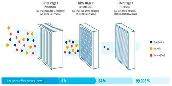
Figure 2.
Working schematic of multi-stage filtration system [43].
In the initial stage of the filtration process, pocket filters are employed to effectively capture larger particles (PM10), such as dust and pollen, from the air supply and recirculation in air conditioning systems. These filters are energy-efficient due to their low-pressure drop. The subsequent stage focuses on filtering the majority of PM2.5 particles. Cassette filters are particularly advantageous in this stage, as they possess a high dust-holding capacity and consistently efficient particle separation. The final stage aims to maintain cleanliness and sterility in the indoor air by utilizing HEPA filters. HEPA filters, specifically those classified as H14, exhibit high efficiency in eliminating over 99.995% [43] of particles, germs, and viruses from the air. This greatly reduces the risk of indoor infections [44].
Multi-stage filtration systems integrated into air conditioning systems play a pivotal role in improving IAQ by effectively capturing a diverse range of airborne particles. To optimize the performance of air conditioning systems equipped with multi-stage filtration, it is essential to ensure appropriate system design, regular maintenance, and careful consideration of the associated energy implications [45].
2.2.3. ACs with Activated Carbon Filter
Activated carbon air filters contain a bed of carbon enclosed in a cloth or mesh material, as shown in Figure 3. These filters effectively purify the air by eliminating gaseous compounds. Standard air filters are unable to capture small molecules such as odors and volatile organic compounds (VOCs), allowing them to pass through. However, activated carbon filters are designed to trap and remove these molecules from the indoor air, thereby enhancing the air quality in your home [46].
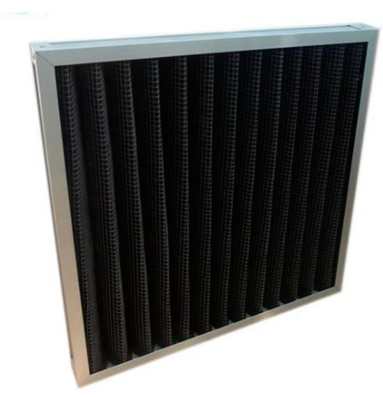
Figure 3.
Air conditioning system active carbon filter [47].
Air conditioning systems can be enhanced to improve IAQ by incorporating activated carbon filters. These filters, also known as activated charcoal, consist of a highly porous material with a large surface area for adsorption. They are effective in trapping and adsorbing various pollutants, including PM2.5 particles, gaseous pollutants, odors, and volatile organic compounds (VOCs), thus efficiently eliminating them from the indoor air circulated by the air conditioning system. By utilizing activated carbon filters in air conditioning systems, IAQ can be improved by addressing specific airborne pollutants that standard particulate filters may not effectively capture [48], as shown in Table 7.
Table 7.
Low-energy occupant-responsive Heating, Ventilation and Air Conditioning (HVAC) controls and systems project summary [49].
This project introduces a groundbreaking advancement in HVAC systems by integrating energy-efficient personal comfort system (PCS) and innovative variable air volume (VAV) technology enhancements. The integration aims to transform how heating and cooling are managed in commercial offices, prioritizing energy efficiency and occupant comfort. By combining localized heating and cooling solutions with novel time-averaged ventilation (TAV) techniques, precise control over comfort levels and substantial energy savings are targeted. The project includes the development of open-source control software for comprehensive system management, validated through practical field studies featuring energy-efficient PCS chairs, as shown in Table 8. The incorporation of TAV into industry guidelines and the introduction of energy management software stand out as significant contributions, with potential to greatly reduce natural gas and electricity consumption, prompting a reevaluation of HVAC control standards and occupant comfort in commercial spaces.
Table 8.
Low-cost Micro-electromechanical system (MEMS)-based ultrasonic airflow sensors for rooms and HVAC systems project summary [50].
The approach to critical analysis based on the provided information involves a thorough assessment of the project’s objectives, significance, research methodology, and anticipated outcomes to determine its feasibility and potential impact. This entails evaluating the alignment between the identified problem and the proposed solution, as well as gauging the practicality of utilizing emerging MEMS technologies for airflow sensing. Furthermore, the scalability of the project’s innovations for real-world applications is considered. Alongside this, a careful examination of the projected benefits, such as improved energy efficiency and indoor comfort, is weighed against potential challenges like technological constraints, integration complexities, and market reception. This methodical approach aims to ensure the project’s objectives are well-founded, the chosen research methodologies are robust, and the expected outcomes align not only with the needs of the HVAC industry but also with the standards set by energy committees.
2.3. Indoor Air Quality Assessment
The study investigates the current methodological framework applied to the development of indoor air quality assessment of buildings. Hassan et al. (2024) studied the effects of deep energy renovations (DERs) on indoor air quality (IAQ), ventilation, and thermal comfort in 12 Irish homes [51]. The study was conducted in three different locations, namely, urban, suburban, and rural areas across Ireland, to investigate the effects of pre- and post-renovation measurements of indoor air pollutants such as PM2.5, CO2, CO, formaldehyde, radon, NO2, and Benzene, toluene, ethylbenzene, xylenes as BTEX, along with assessments of the newly installed mechanical ventilation systems. The in situ measurements were recorded between May 2019 and January 2020, with post-retrofit measurements resuming from November 2022 to June 2023 due to COVID-19 restrictions. It was found that the DERs could result in improvements in thermal comfort, with homes being significantly warmer (p < 0.0001), and having better ventilation, as indicated by improved CO2 concentrations. However, some bedrooms remained under-ventilated, and concentrations of PM2.5 (p < 0.0001) and formaldehyde (p < 0.05) increased during the post-retrofit. These increases were attributed to factors like inadequate ventilation, outdoor air ingress, and occupant activities. The study highlighted the need for proper installation and maintenance of ventilation systems and emphasized the importance of pollutant source control to ensure sustainable and healthy homes during the post-retrofit. The study findings suggested that further research is required to explore the impact of occupant behavior and the effectiveness of ventilation systems in real-world conditions, as well as to promote public awareness of the importance of ventilation in energy-efficient homes.
Sha et al. (2024) introduced a novel data mining approach to uncover associations and sequences between indoor air quality (IAQ), HVAC operations, and occupant activities. The study was conducted using datasets from 70 residential houses and a single commercial building [52]. The study developed a peak detection method and extended rule mining criteria to analyze pollutant concentration peaks and their temporal relationships with HVAC operation and occupant behavior. The peak detection method was employed by moving windows and non-maximum suppression to identify and filter pollutant peaks. The rule mining method was extended to use a multi-criteria decision-making tool to include time lags and co-occurrence of events thus providing insights into sequential patterns. The results showed a high accuracy rate of 93.19% in detecting pollutant peaks. Significant temporal patterns were also found, such as CO2 peaks frequently occurring at specific times (e.g., 12:00, 17:00, and 19:00 to 24:00) and within the two hours following increased occupant activities or high Wi-Fi usage in commercial buildings. These findings suggested that occupant activities can significantly influence IAQ, supporting the development of more effective control strategies for HVAC systems to optimize indoor air quality.
Takebayashi (2022) investigated the impacts of urban heat islands (UHIs) on thermal comfort in the coastal cities of Tokyo, Osaka, and Nagoya. The study used the Mesoscale Weather Research and Forecasting Model (WRF) approach to analyze thermal environmental indices over August 2010 [53]. The study was focused on the effects of sea breezes on indoor cooling loads and heat stroke risks. It was found that, despite high humidity near the coastline areas, low air temperatures and high wind velocities could result in lower thermal indices such as Wet-Bulb Ground Temperature (WBGT), Set Point Temperature (SET), and The Physiological Equivalent Temperature (PET). According to environmental forecasting, outdoor temperatures decreased by approximately 1.5–3.6 °C, SET by 1.4–3.4 °C, and WBGT by 0.1–0.6 °C while assessing temperature variations from inland to coastal areas. To avoid the risk of the UHI effect in densely built urban areas, the study found that solar shading has proven more effective in mitigating heat compared to other methods like urban ventilation and mist spray. This research highlights the nuanced relationship between temperature, humidity, wind velocity, and urban planning, suggesting that more detailed discussions at smaller scales are needed.
Jara-Baeza et al. (2023) evaluated residents’ perceptions of indoor environmental quality (IEQ) in high-rise social housing in Melbourne [54]. Data were collected through surveys from 94 apartment units across 38 buildings between May 2021 and May 2022. Key IEQ parameters were assessed including thermal comfort, indoor air quality (IAQ), lighting, and acoustics. The study found that residents were least satisfied with indoor temperature in summer (33%) and most satisfied with daylight (72%). Noise was identified as the most influential factor on overall IEQ satisfaction, despite being rated as the second least important. High levels of outdoor noise were linked to sleep disturbances (61.8%) and restricted window use for ventilation (43.4%). Over 54% of residents reported health issues, with older age groups being more affected. The study highlighted the need for the tailored weighting of IEQ parameters and the importance of addressing overheating in summer. The findings emphasized the effectiveness of appropriate fenestration design and ventilation in improving thermal satisfaction and IAQ.
Belais and Licina (2023) assessed the impact of outdoor air pollution on the efficiency of residential ventilative cooling (VC) across 26 European cities. The study used a dataset of five outdoor air pollutants (PM2.5, PM10, O3, NO2, and SO2) collected from 182 measurement stations over a five-year period between 2015 and 2019 [55]. The study was employed in building energy simulations to evaluate VC potential. The results revealed that VC could reduce cooling demand by 17% to 100% depending on local climate and pollution levels. However, urban air pollution reduced VC potential by an average of 24%, with reductions ranging from 13% in suburban areas to 44% in densely built urban locations. The study identified PM2.5 and PM10 as significant limiting factors across all locations, while NO2 and O3 were found to be critical in urban areas, respectively. The findings highlighted the importance of considering air pollution in the design and operation of ventilative cooling systems to enhance building sustainability and human health.
An and Chen (2023) developed a deep reinforcement learning (DRL) controller to optimize indoor air quality and thermal comfort while minimizing energy consumption [56]. The study adopted a room model based on 3-week monitoring data to train a deep Q-network (DQN) algorithm, which was then implemented in a smart indoor environmental control system. Field testing over four days demonstrated that the DQN controller improved PM2.5 healthy periods and thermal comfort by approximately 21% and 16%, respectively, while reducing energy consumption by 23% compared to a baseline occupant-based controller. The controller’s effectiveness was also validated in different rooms, showcasing its robust performance in managing indoor PM2.5, thermal comfort, and energy efficiency. Colclough and Salaris (2024) examined the prevalence of overheating in 57 nearly-zero energy buildings (nZEBs) across Ireland, including 44 passive houses [57]. The study assessed compliance with overheating criteria from Chartered Institution of Building Services Engineers (CIBSE) TM59, Passive House Institute, and WHO. The outdoor temperature data were collected between 2016 and 2021 via various sensors. The study found that 26% of new builds exceeded the CIBSE TM59 criteria, while 48% of average temperatures surpassed the World Health Organization (WHO) recommendations by at least 10% of the year. However, it was found that only 4% of newly built passive houses and 5% of retrofitted homes failed to meet their respective criteria. The study highlighted the divergence in overheating assessments between different standards and emphasized issues with poorly installed heat pumps and inadequate shading. The study recommended a national strategy to address overheating risks, considering the increasing number of nZEB homes and the effects of climate change.
Arriazu-Ramos et al. (2023) showed the impact of climate scenarios on indoor overheating hours (IOHs) in residential buildings with a focus on natural ventilation. The empirical study was conducted in two neighborhoods in Northern Spain. The study employed building energy simulations for a typical meteorological year and an extreme warm summer to assess IOHs [58]. The study findings indicated the significant increase shown during the heatwave in 2022, with the mean IOHs reaching 2.97% in one neighborhood and 3.85% in another, and over 30% in the most affected buildings. The study highlighted that microclimate effects could increase an average of 7.52% in extreme conditions. Berneiser et al. (2024) conducted an in-depth analysis of ventilation practices and mechanical ventilation systems in Germany [59]. The study focused on exploring discrepancies between thermal properties of buildings and occupants’ behavior. The study adopted a mixed-method approach, which consisted of qualitative interviews (N = 10) and a nationwide online survey (N = 952), in order to gather data on indoor climate needs and ventilation practices. The study highlighted the necessity of integrating occupants’ needs into the mechanical ventilation system design to balance energy efficiency with user satisfaction.
3. Materials and Methods
3.1. Site Description
This study focuses on Lahore, Pakistan, considered the country’s most polluted city, which is located in Punjab, where continuous efforts are being made to improve the IAQ. The study area is distinguished by densely populated districts and various building types, such as houses, apartments, schools, offices, and hospitals with limited ventilation, all influencing IAQ. It lies in the BSh. subtropical steppe zone of the Köppen–Geiger climate classification zones, as shown in Figure 4 [60]. This climate subtype is characterized by its location in subtropical regions and its relatively dry conditions. The “B” in BSh represents a dry climate, while the “S” indicates that it is a subtropical climate. The “h” signifies a hot climate. In the BSh climate zone, temperatures are generally high throughout the year. Summers in Lahore are extremely hot, with average temperatures reaching around 40 °C or even higher in some cases. Winters are mild and short, with average temperatures of around 15–20 °C.
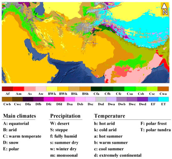
Figure 4.
Köppen–Geiger climate classification map, Lahore, Pakistan [52].
3.2. Conceptual Framework
The adopted methodology for our research is a mixed method strategy, incorporating both qualitative and quantitative approaches, as shown in Figure 5. To address the issue of improving IAQ in Pakistan, we have utilized the widely adopted method of air conditioning systems, commonly employed in developed countries. In order to gain a comprehensive understanding of the urban regions in Pakistan, the study employed the CLIMA tool (version 0.8.17), which offers a range of valuable insights such as climate summaries, temperature and humidity data, psychometric charts, and natural ventilation patterns [61].

Figure 5.
Flow design of conceptual framework. Drawn by author.
After analyzing the gathered dataset, we will then compare it with the proposed air conditioning system method using the ASHRAE Global Thermal Comfort Database II visualization. This approach aims to enhance the IAQ in urban regions of Pakistan. One notable advantage of employing air conditioning systems is their ability to regulate humidity levels effectively while providing efficient cooling and ensuring thermal comfort within indoor environments. Table 9 delineates the pros and cons of the adopted methodological framework for the present study.
Table 9.
Pros and cons of conceptual framework.
3.3. Tool and Database
This research utilized two key resources: the Center of the Built Environment (CBE) CLIMA Tool and the ASHRAE Global Thermal Comfort Database II version 2.1. The CBE CLIMA Tool was employed to extract various parameters including climate summaries, temperature and humidity data, psychometric charts, natural ventilation patterns, and heat stress maps. These parameters were essential for the research analysis. Furthermore, the ASHRAE Global Thermal Comfort Database II was utilized to obtain datasets and plots related to building types, satisfaction metrics, and conditioning types for indoor thermal comfort. These datasets and plots were integral for evaluating and understanding indoor thermal comfort in the research.
The CBE CLIMA Tool is an open-source web application that enables architects and engineers to effectively analyze and visualize climate data for climate-adapted building design. It offers a user-friendly interface with an interactive world map as the main landing page. Through this map, users can access a vast collection of publicly available weather data files. These files are sourced from reputable repositories such as EnergyPlus and Climate.OneBuilding.org. Additionally, users have the flexibility to upload their own valid Energy Plus Weather (EPW) files for data analysis. The tool not only provides data visualization but also facilitates data organization, manipulation, and interpretation in a straightforward manner [62].
The ASHRAE Global Thermal Comfort Database II, also known as the Comfort Database, is an online and open-source resource that contains comprehensive datasets of objective indoor climatic observations, along with corresponding subjective evaluations provided by the building occupants who experienced those conditions. The primary purpose of this database is to facilitate diverse research inquiries regarding thermal comfort in real-world settings. It offers a user-friendly web interface that allows users to apply various filters based on multiple criteria. These criteria include building typology, occupancy type, demographic variables of subjects, subjective thermal comfort states, indoor thermal environmental criteria, calculated comfort indices, environmental control criteria, and outdoor meteorological information. Additionally, a web-based interactive tool has been developed to visualize thermal comfort, providing end-users with a quick and interactive way to explore the data [63].
3.4. Data Acquisition
In this study, the Statistical Analysis in Social Science (SPSS) software v.29 was used to conduct the statistical analysis. Checking a dataset for invalid cases or values is a critical part of data preparation. Invalid data points are observations that reflect inaccurate, inattentive, or careless response values. Cases that exhibit these types of responses can seriously bias a study. The appropriate procedure for handling invalid data is typically the removal of the data in the invalid case, which often results in a reduction in sample size. Impossible values refer to values in a variable that lie outside the theoretical range for that particular variable, for example: a case with a negative value for body mass index (BMI) would be impossible. Unless the convention recommends that the researcher go back to the original source (e.g., the questionnaire survey) and confirm the correct value, it is recommended that these values be set as missing values. In the present study, an impossible wet bulb temperature of 48.50 °C was corrected to 25.60 °C. A response subset is representative with respect to the sample if response propensities are the same for all units in the population.
The response of a unit is independent of the response of all other units, which denotes the response of unit i and is an indicator showing whether a unit took part in the survey. Strong representativeness corresponds to the missing completely at random (MCAR) pattern for every target variable y. This means that non-response does not cause estimators to be biased. Although this definition is appealing, its validity can never be tested in practice. To solve this problem, a weaker definition of representativeness was introduced.
3.5. Data Mining
In this study, it was found that the data were missing completely at random (MCAR). After preparing the data for analysis, it was observed that out of 100 recorded cases, 98 cases contained missing data (98.0%) and, out of 53 variables, 2 variables contained missing data (2.8%), which amounted to a total of 0.04% missing information in the dataset. To assess whether the pattern of missing values was MCAR, Little’s MCAR test was conducted. The null hypothesis of Little’s MCAR test is that the pattern of the data is MCAR and follows a chi-squared distribution. Using an expectation–maximization algorithm, the MCAR test estimates the univariate means and correlations for each of the variables, as shown in Figure 6a,b.

Figure 6.
(a) Input variables selected to complete the data mining process. (b) Missing patterns were excluded from the dataset.
The results revealed that the pattern of missing values in the data was MCAR: χ2 (104) = 121.645, p = 0.114. Even though the proportion of the total missing data is less than 5% and the data are MCAR, the final sample size may still be affected by listwise or pairwise deletion when the analysis is run. Listwise deletion removes a case if a case has any missing value for any of the variables used in an analysis. The missing values of data allow flexibility when addressing missing data because the proportion of missing data in the sample is less than 5% and the pattern of missing data is MCAR. Based upon these two findings, the data should be fine using either pairwise or listwise deletion methods. Listwise and pairwise deletion are unbiased techniques when data are MCAR; however, pairwise deletion increases the power.
4. Analysis and Results
4.1. Adaptive Thermal Comfort
After extracting the data from the EPW file of the Lahore (Pakistan) weather station from Climate.OneBuilding.Org, it was uploaded to the CLIMA tool. The obtained data were then compared with the ASHRAE Global Thermal Comfort Database II using the proposed methodology. The resulting measurements and comparisons are outlined in Figure 7.
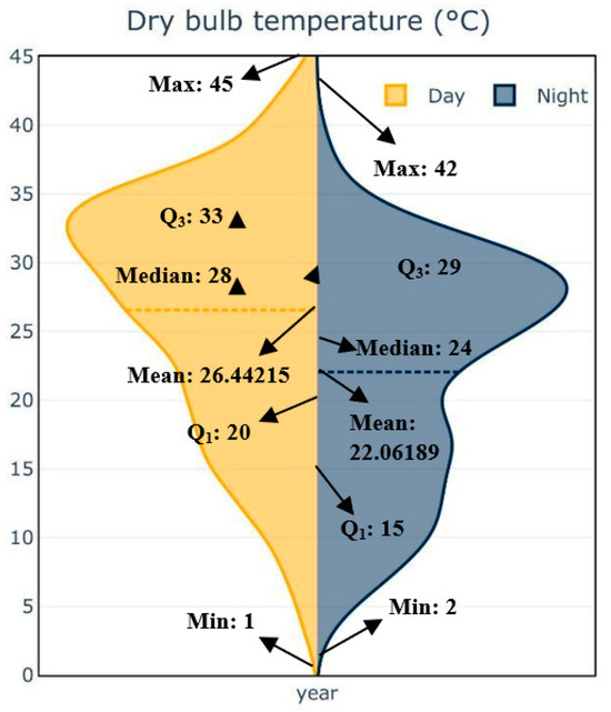
Figure 7.
Dry bulb temperature during day- and night-time. Data source: https://clima.cbe.berkeley.edu (accessed on 25 March 2024).
The left side of the graph in Figure 7 illustrates the variation in daytime dry bulb temperatures in the Lahore region over the course of a year. The vertical axis represents the temperature in degrees Celsius, while the horizontal axis represents time in years. From the graph, we can observe that the highest recorded temperature during the year is 45 °C, while the lowest recorded temperature is 1 °C. These values represent the extreme points on the graph. To better understand the overall temperature trend, we can look at the measures of central tendency. The mean temperature, which is the average of all the temperature values on the graph, is calculated to be 26.55 °C.
The mean is influenced by extreme values, so, in this case, it considers both the high and low temperature extremes. Another measure we can consider is the median temperature, which is the middle value when all the temperature values are arranged in ascending order. In this case, the median temperature is 28 °C. Unlike the mean, the median is not affected by extreme values, providing a representation of the temperature that is more typical or representative of the data. Additionally, we can examine the quartiles of the data. The first quartile, denoted as Q1, is 20 °C, indicating that 25% of the temperature readings on the graph fall below this value. It represents the boundary between the lowest 25% of the data and the upper 75%. On the other hand, the third quartile, denoted as Q3, is 33 °C, representing the boundary between the lowest 75% of the data and the upper 25%. In other words, 75% of the temperature readings on the graph fall below this value.
Based on the analysis of daytime dry bulb temperature data in the Lahore region indicates that extreme temperatures are prevalent, with a recorded high of 45 °C and a low of 1 °C. However, the measures of central tendency, such as the mean temperature of 26.55 °C and the median temperature of 28 °C, suggest that the overall temperature trend is moderately warm. This raises the question of whether the extreme temperature values are outliers or if they represent a significant climatic event. Further investigation into the factors influencing temperature extremes in this region is warranted to better understand their implications for local climate patterns and potential impacts on human activities and ecosystems.
The right side of the graph in Figure 7 illustrates the nighttime dry bulb temperatures in Lahore throughout the year. The y-axis represents the temperature in degrees Celsius, while the x-axis represents the time in years. Upon closer examination of the graph, it becomes evident that the highest recorded nighttime temperature throughout the year is 42 °C, whereas the lowest recorded temperature is 2 °C. To gain insights into the typical temperature characteristics, we can analyze the measures of central tendency. The mean temperature, calculated by summing all the temperature values on the graph and dividing them by the total number of values, is determined to be 22.0 °C.
The mean is influenced by extreme values, considering both the highest and lowest temperature points. In contrast, the median temperature, which represents the middle value when the temperature values are arranged in ascending order, is found to be 24 °C. Unlike the mean, the median is not influenced by extreme values and provides a representation of the central or typical temperature reading. Furthermore, we can explore the quartiles of the data. The first quartile, denoted as Q1, has a value of 15.5 °C, indicating that 25% of the temperature readings fall below this value. Q1 marks the boundary between the lowest 25% of the data and the upper 75%. On the other hand, the third quartile, denoted as Q3, has a value of 29 °C, signifying that 75% of the temperature readings fall below this value. Q3 represents the boundary between the lowest 75% of the data and the upper 25%. This prompts the question of whether the extreme temperature values are exceptional events or if they reflect noteworthy nocturnal climatic patterns. By considering these statistical measures, we can gain a more comprehensive understanding of the day and nighttime temperature distribution and trends in the Lahore region throughout the year, as shown in Table 10.
Table 10.
Descriptive statistics of dry bulb temperature throughout the year, Lahore [64].
In Lahore, the dry bulb temperature exhibits variations throughout the year, as shown in Table 10 and the accompanying graphs. The data highlights that the temperature range within which people feel comfortable thermally is between 18 °C and 24 °C. During the winter season (December, January, and February), individuals may experience a slight sensation of cold. Conversely, from May to September, which corresponds to the summer season, the temperature exceeds 40 °C, significantly surpassing the ASHRAE adaptive comfort limit of 24.5 °C. This raises concerns about the impact of these extreme temperatures on human health, well-being, and productivity, as well as the potential implications for energy consumption and the need for adaptive measures in buildings and urban planning.
In Figure 8, along the x-axis, outdoor relative humidity is depicted, while age is represented on the y-axis. In the context of a figure comparing outdoor relative humidity and age, the circle’s dimensions symbolize the population count within each age category corresponding to the given humidity level. The plot reveals a discernible positive correlation between outdoor relative humidity and age. This inference implies that, as outdoor relative humidity escalates, there is a concurrent elevation in the average age of the populace. This trend can be attributed to the heightened vulnerability of older individuals to humidity-induced effects, encompassing health challenges like heat-related ailments and respiratory issues.

Figure 8.
Bubble plot of age and relative humidity. Data source: https://repository.uel.ac.uk/item/8q774 (accessed on 25 March 2024).
In an overarching analysis, the plot substantiates the existence of a moderate correlation between outdoor relative humidity and age, predominantly owing to the increased susceptibility of older demographics to humidity-related implications. It is noteworthy that the climatic range considered comfortable for this locale falls within the 40% to 60% humidity threshold. Upon closer scrutiny of the bubbles, it is evident that a substantial majority of observations fall within this comfortable humidity range, depicted as the shaded gray segment within the visualization, accompanied by a few outliers. The visualization exhibits numerous sizable bubbles aligning with age points spanning from 40 to 60 years and outdoor relative humidity ranging between 40% and 60%. This indicates a notable concentration of individuals within the 40–60 age bracket experiencing relative humidity levels within the 40–60% range [65].
The presented Figure 8 highlights a notable positive correlation between outdoor relative humidity and age. This suggests that elevated humidity levels coincide with an increase in the average age of the population. This relationship can be logically attributed to the heightened susceptibility of older individuals to health issues arising from humidity, such as heat-related ailments and respiratory concerns. The visualization further emphasizes that a significant portion of the population falls within the accepted comfortable humidity range of 40% to 60%, as indicated by the prominent gray shading in the plot. Nonetheless, the presence of a few outliers necessitates a more in-depth exploration into potential factors contributing to these deviations from the observed trend. Moreover, the clustering of larger bubbles around the age range of 40 to 60 and within the 40–60% humidity bracket indicates a substantial demographic of individuals aged 40 to 60 years who are exposed to humidity levels falling within the comfort range. This comprehensive analysis encourages a consideration of the intricate interplay among age, humidity, and associated health implications. It is important to acknowledge the significance of these outliers, as they may introduce complexities to the established correlation.
The presented graph in Figure 9 depicts the annual variation in relative humidity in Lahore. It showcases the monthly distribution of humidity levels throughout the year, with the vertical axis representing the percentage of relative humidity and the horizontal axis indicating the months from January to December. The graph highlights that the recorded maximum humidity value reaches 100%, while the minimum value stands at 16%. Notably, the graph incorporates distinct color schemes: the gray section represents the range of humidity considered comfortable, the blue color denotes the overall range of relative humidity, and the sky-blue shade indicates the average relative humidity for the region over the year. The graph suggests that relative humidity becomes a significant concern for individuals, particularly from July to October, posing challenges for indoor comfort. These findings raise important questions about the impact of high humidity levels on human health, comfort, and productivity, as well as the need for effective indoor humidity control strategies and building design considerations.
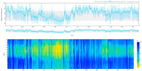
Figure 9.
Yearly relative humidity chart for Lahore. Data source: https://clima.cbe.berkeley.edu (accessed on 25 March 2024).
This graph in Figure 10 is a psychometric chart [66], illustrating the characteristics of the case study location. It visualizes the relationship between temperature and humidity ratio. The y-axis represents the humidity ratio measured in grams of water per kilogram of air, while the x-axis represents temperature in degrees Celsius. The chart also includes a color-coded band indicating different temperature ranges.

Figure 10.
Psychometric chart. Data source: https://clima.cbe.berkeley.edu (accessed on 25 March 2024).
When examining the graph from left to right, it shows a progression from low sensible heat to high sensible heat, indicating an increase in temperature. Moving from bottom to top on the graph signifies an increase in absolute humidity or humidity ratio, reflecting a higher amount of moisture in the air per kilogram of dry air.
Based on the data points on the graph, we can infer that when the temperature is kept constant, the humidity ratio in the air also increases, and vice versa. The blue dots on the graph represent the winter season, with maximum temperatures around 17–18 °C, while the red and yellow dots correspond to the summer season, characterized by maximum temperatures reaching approximately 45 °C in the specific case study location. These results pose important questions about the impact of temperature and humidity ratio variations on indoor thermal comfort and energy efficiency. This research argument revolves around exploring effective strategies for managing temperature and humidity levels within indoor environments, particularly during the summer season with extreme temperatures.
The bar chart represented in Figure 11 shows the annual natural ventilation [67] levels at the case study location. The x-axis represents the months of the year, ranging from January to December, while the y-axis displays the percentage of natural ventilation. Analysis of the graph reveals a concerning issue from May to September, where there is a significant decrease in natural ventilation. Consequently, these months pose significant challenges for indoor occupants, as there is minimal airflow, and it becomes increasingly uncomfortable to stay indoors during this period. The discovery suggests that there is limited air movement during these months, creating difficulties for individuals indoors in terms of IAQ, thermal comfort, and general wellness. This highlights the importance of additional research to explore the specific factors that contribute to reduced natural ventilation during this period, including weather patterns, building design [68] and orientation, and potential obstacles to airflow. Understanding the causes and consequences of diminished natural ventilation is essential for developing effective approaches to improve IAQ and comfort, address potential health risks associated with inadequate ventilation, and optimize energy-efficient ventilation systems in buildings within the studied location.

Figure 11.
Natural ventilation yearly bar Chart. Data source: https://clima.cbe.berkeley.edu (accesses on 25 March 2024).
This chart displayed in Figure 12 is the distribution of thermal stress based on Universal Thermal Climate Index (UTCI) [62,63] throughout the year. The x-axis represents the months from January to December, while the y-axis shows the percentage of thermal stress distribution. Different colors in the color-coded band indicate various levels of thermal stress, with maroon indicating extreme heat stress. Upon closer examination of the graph, it becomes evident that, from April to October, there is a significant prevalence of extreme or very strong heat stress. This poses a high risk of heat stroke for occupants staying indoors during these months. Additionally, the chart reveals a concerning pattern of minimal or negligible no thermal stress, indicating a challenging situation at the case study location. These findings bring up crucial inquiries concerning the consequences of long-term exposure to extreme heat stress on human well-being, productivity, and overall quality of life. It is imperative to examine the factors that contribute to the high occurrence of extreme heat stress, including local climate conditions, urban heat island effects, building design, and indoor heat mitigation strategies. Moreover, exploring effective adaptation measures, such as thermal insulation, shading techniques, and active cooling systems, becomes essential for enhancing indoor thermal comfort, minimizing the risk of heat-related illnesses, and bolstering the resilience of individuals and communities in the studied location.

Figure 12.
Universal thermal climate index (UTCI) heat stress map. Data source: https://clima.cbe.berkeley.edu (accesses on 25 March 2024).
This illustration portrayed in Figure 13 depicts the interrelation between the duration of residency and the outdoor heat stress index. Each bubble within the plot corresponds to an individual, with its size indicative of the person’s outdoor heat stress index. The horizontal axis represents the outdoor heat stress index, while the vertical axis denotes the length of an individual’s residency in the area. The distinctive linear configuration of the figure signifies a direct association between the length of residency and the outdoor heat stress index. This alignment denotes a positive correlation, where an increase in the length of residency is concurrent with a rise in the outdoor heat stress index. This correlation can be attributed to the prolonged exposure of long-term residents to heat stress, potentially leading to a lower level of acclimatization as compared to those who have recently moved to the area.

Figure 13.
Bubble plot between length of residency and outdoor heat stress index. Data source: https://repository.uel.ac.uk/item/8q774 (accessed on 25 March 2024).
The visual representation designates a gray segment within the plot, signifying a comfort zone in terms of outdoor heat stress and duration of residency. Upon closer examination of the plot, it is evident that the bubbles adhere to a shared trajectory, yet the outdoor heat stress index demonstrates an ascending trend. This observation indicates a consistent elevation in the outdoor heat stress index across all individuals, irrespective of their length of residency. Plausible explanations for this phenomenon encompass factors such as an increasingly warmer climate, greater occupational exposure to outdoor conditions, or limited access to cooling amenities.
Figure 13 visualizes the relationship between length of residency and outdoor heat stress index. The linear shape of the plot suggests a positive correlation, indicating that longer residency is associated with higher outdoor heat stress index. This alignment of bubble sizes with the length of residency underscores the notion that individuals who have lived in the area longer tend to experience greater heat stress. However, the observation that all bubbles lie along the same line while the outdoor heat stress index varies suggests that there is a universal increase in heat stress, regardless of residency duration. This could be attributed to broader environmental factors like climate change or societal changes such as increased outdoor work. The shaded comfort zone serves as a valuable benchmark for assessing the extent of heat stress experienced by residents. Further analysis could delve into specific contributing factors that might be driving the uniform rise in heat stress despite differing lengths of residency, considering variables such as urbanization, infrastructure development, and adaptive strategies to cope with rising temperatures.
Figure 14 depicts as a visual representation of outcomes derived from a meta-analysis, illustrating the effects of an intervention across various individual studies. The focal point of analysis is the occupants’ thermal sensation vote (TSV), a metric reflecting individuals’ comfort levels within a given environment. The study’s focus revolves around the influence of outdoor environmental temperature (OET) on this thermal sensation. Within the plot, each square corresponds to an individual study, and its size is proportionate to the study’s weight, signifying its impact on the aggregate outcome. Enclosed within each square is a horizontal line that signifies the OET’s impact on TSV within that particular study. Vertical lines extending from the horizontal lines indicate the confidence intervals for these effects. Notably, the diamond-shaped region within the plot symbolizes the collective effect size, a consolidation of outcomes from all studies. The horizontal lines encompassing this diamond signify the confidence interval for the overall effect size.
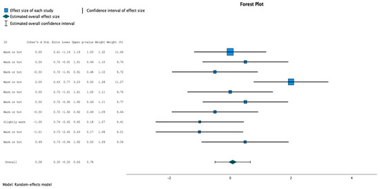
Figure 14.
Forest plot of outdoor air temperature and thermal sensation vote of occupants. Data source: https://repository.uel.ac.uk/item/8q774 (accessed on 25 March 2024).
Observing the findings, the aggregate effect size presents a positive inclination. This suggests a positive correlation between higher OET and elevated TSV, implying increased comfort levels as outdoor temperatures rise. However, the wide span of the confidence interval suggests inherent uncertainty, leaving room for the true effect size to potentially lean either positively or negatively. The positioning of the estimate in relation to the zero-effect line is pivotal. Specifically, if the estimate rests to the left of this line, it indicates a sensation of warmth among the analyzed individuals. Conversely, positioning to the right signals a perception of heat. In the context of this plot, the comprehensive 95% confidence interval for the effect size spans from −0.5 to 0.66. Notably, this interval is skewed toward the warm side, underscoring that individuals within this climatic context tend to experience heightened warmth as outdoor temperatures increase. Moreover, the study’s design reveals that the perceived level of heat remains consistent between day and night. This insight underscores a minimal disparity between outdoor air temperatures during daytime and night-time hours in this specific climate.
The analysis involves a thorough evaluation of a meta-analysis on the relationship between outdoor temperature and occupants’ thermal comfort ratings. The overall findings suggest a positive link between higher outdoor temperatures and more favorable thermal comfort. However, the wide confidence interval highlights uncertainty. The observed positive effect within this range indicates increased comfort with higher temperatures, but the possibility of a contrary effect should be considered. The symmetric distribution of the confidence interval around the null point suggests potential for heightened warmth perception with rising outdoor temperatures. Contextual factors like humidity, clothing choices, and individual preferences should be carefully considered. The consistent warmth perception regardless of time of day emphasizes the need to explore local climate, building design, and adaptive behaviors. Overall, recognizing the complexity of thermal comfort perception and acknowledging study limitations is crucial.
The dataset referenced in citation [57] pertains to Famagusta in Cyprus. Its applicability to regions within Pakistan is grounded in the similarity of climatic conditions, specifically characterized by hot and humid weather.
4.2. Obtained Datasets from ASHRAE Global Thermal Comfort Database II
The box plot in Figure 15 represents the distribution of indoor air temperature in various settings such as houses, classrooms, and offices, based on different conditioning methods: air conditioning, mixed mode, and natural ventilation. The focus of the analysis is on the occupants’ comfort level.

Figure 15.
Boxplot for the distribution of indoor air temperature. Data source: https://cbe-berkeley.shinyapps.io/comfortdatabase/ (accessed on 25 March 2024).
Upon examining the box plot, it becomes evident that the dataset contains numerous outliers, indicating some extreme temperature values that deviate from the norm. Additionally, when considering the average temperature, it is noticeable that the lower quartile is closer to the mean than the upper quartile, suggesting a positive skew in the data distribution. This skewness is further supported by the length of the upper whisker being longer than the lower whisker [69,70,71]. Most of the data points fall within the range of 23 °C to 27 °C, indicating that most indoor environments are maintained within this temperature range to ensure comfort for the occupants while using these conditioning types.
These findings prompt significant inquiries concerning the efficiency of various methods for achieving and sustaining thermal comfort. It is vital to investigate the factors that contribute to the occurrence of extreme temperature values and outliers, including variations in building design, equipment efficiency, occupant behavior, and control systems. Additionally, exploring strategies to enhance temperature control and thermal comfort, such as optimizing conditioning systems, employing energy-efficient design principles, and adopting occupant-centered approaches, becomes essential. These efforts aim to improve the overall indoor comfort experience and well-being of occupants across different environments.
This box plot in Figure 16 visualizes the distribution of predicted mean vote (PMV) [72] values in houses, classrooms, and offices, considering different types of conditioning methods: air conditioning, mixed mode, and natural ventilation. The main objective is to examine the comfort level experienced by occupants in these settings.
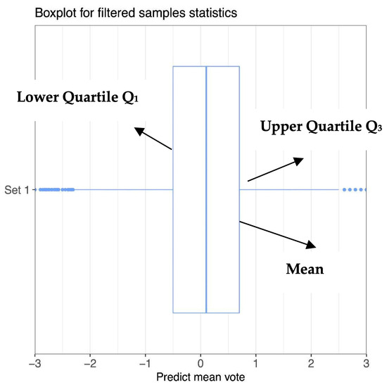
Figure 16.
Boxplot for the distribution of PMV values. Data source: https://cbe-berkeley.shinyapps.io/comfortdatabase/ (accessed on 25 March 2024).
Upon analyzing the box plot, it becomes apparent that the dataset contains outliers, indicating the presence of a few PMV values that significantly deviate from the overall trend. When looking at the central tendency of the data, we observe that the mean is positioned equidistant from both the lower and upper quartiles, suggesting a symmetrical distribution. This symmetry is further supported by the similar lengths of the upper and lower whiskers.
The majority of PMV values cluster within the range of −0.5 to +0.7, indicating that occupants generally perceive a neutral thermal sensation within this interval. This suggests that the different conditioning methods employed in these environments effectively provide a comfortable indoor experience, where individuals do not experience extreme sensations of either heat or cold.
This scatter plot in Figure 17 depicts the relationship between indoor air temperature and PMV (predicted mean vote) in classrooms and offices with different conditioning types: air conditioning, mixed mode, and natural ventilation. The Y-axis represents PMV values, ranging from −3 (cold sensation) to +3 (hot sensation), with zero indicating a neutral thermal sensation. The X-axis represents indoor air temperature in °C. The plot shows a modest positive correlation between the variables, indicating that as one variable increases, the other tends to increase as well, and vice versa. Within the temperature range of 20 °C to 25 °C, the data points cluster around PMV values close to zero, indicating a state of thermal comfort. However, as the temperature exceeds 25 °C, the positive correlation suggests an upward trend in PMV values and an associated increase in UTCI heat stress. It is important to note the presence of a few outliers in the dataset. These research findings suggest the importance of maintaining indoor air temperatures within the range of 20 °C to 25 °C to achieve optimal thermal comfort for occupants. However, exceeding this range can lead to discomfort and potentially pose health risks associated with heat stress. Additionally, it is crucial to explore effective strategies for mitigating heat stress and improving thermal comfort. This includes investigating adaptive thermal comfort models, advanced control systems, and personalized comfort solutions. These approaches are essential to ensure the well-being and productivity of occupants across various types of conditioning and settings.
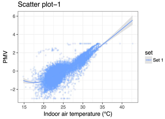
Figure 17.
Scatter plot relationship between PMV and indoor air temperature. Data source: https://cbe-berkeley.shinyapps.io/comfortdatabase/ (accessed on 25 March 2024).
This scatter plot in Figure 18 illustrates the relationship between thermal sensation and indoor air temperature, considering different conditioning types such as air conditioning, mixed mode, and natural ventilation. The observations were conducted in classrooms and offices. The y-axis represents thermal sensation values, ranging from −3 (feeling cold) to +3 (feeling hot), with zero indicating a neutral thermal sensation. The x-axis represents indoor air temperature in °C.

Figure 18.
Scatter plot relationship between TSV and indoor air temperature. Data source: https://cbe-berkeley.shinyapps.io/comfortdatabase/ (accessed on 25 March 2024).
The graph indicates a positive correlation between the two variables in the temperature range of 17 °C to 25 °C. This implies that, as one variable increases, the other also tends to increase, and vice versa. For the temperature range of 25 °C to 30 °C, there appears to be no significant relationship between the variables. However, beyond 30 °C, the positive correlation resumes.
During the initial positive correlation range of 20 °C to 25 °C, the data suggest a prevalence of neutral thermal sensation, indicating that people generally feel thermally comfortable within this temperature range [72]. As the temperature exceeds this range, the positive correlation indicates an increase in neutral thermal sensation, along with a rise in UTCI heat stress. It is worth noting that the dataset contains some outliers as well [73].
The graph in Figure 19 displays the ASHRAE adaptive model [74], where acceptability is used as the satisfaction metric. The x-axis represents the average monthly outdoor temperature in °C, while the y-axis represents the indoor radiant temperature in °C. The graph includes a satisfaction band that spans from zero percent (pink color) to 100 percent (green color). The data were gathered from various building types such as houses, classrooms, and offices, employing different conditioning methods like air conditioning, mixed mode, and natural ventilation [75,76].
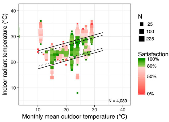
Figure 19.
ASHRAE thermal comfort adaptive model between indoor radiant temperature and monthly mean outdoor temperature. Data source: https://cbe-berkeley.shinyapps.io/comfortdatabase/ (accessed on 25 March 2024).
The graph reveals a positive correlation between the two variables, indicating that, as one variable increases, the other also tends to increase, and vice versa. The solid black line represents the ASHRAE 55 comfort zone. Upon closer examination, it is evident that the majority of the datasets fall within this comfort zone when using the specified conditioning methods [77].
Furthermore, the green datasets on the graph signify that most individuals feel thermally comfortable when the outdoor temperature is around 23 °C, with an indoor radiant temperature range of 17 °C to 27 °C. However, it is important to acknowledge that the dataset contains some outliers as well. This information suggests that optimizing indoor conditions, such as radiant temperature, based on the ASHRAE adaptive model [78], can enhance occupant satisfaction and thermal comfort in various building types and under different conditioning methods.
This plot in Figure 20 serves as a summary of the various plots and datasets described earlier. It illustrates the relationship between PMV, plotted on the x-axis, and the percentage of people dissatisfied. The graph exhibits a general curve represented by a black line. The curve begins at a PMV value of −3, indicating 100% dissatisfaction. As the PMV value increases from −3 to 0, the plot demonstrates a negative correlation with the percentage of dissatisfied individuals. At a PMV value of zero, the percentage of dissatisfaction approaches zero, indicating that PMV zero represents a neutral thermal sensation [79], where nearly all individuals feel thermally comfortable. From 0 to +3 PMV value, the plot shows a positive correlation between the two variables, indicating that at a PMV value of 3, considered a hot sensation, the percentage of dissatisfied individuals is 100%.
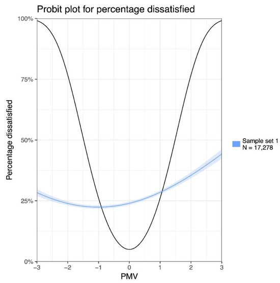
Figure 20.
Satisfaction graph between PMV and percentage dissatisfied. Data source: https://cbe-berkeley.shinyapps.io/comfortdatabase/ (accessed on 25 March 2024).
Now, examining the obtained datasets represented by a blue line, different conditioning types such as air conditioning systems, mixed modes, and natural ventilation systems were used in various building types including houses, classrooms, and offices, with the satisfaction metric set as comfort. The datasets demonstrate that, using these conditioning types, starting from a PMV value of −3, the percentage of dissatisfied individuals is slightly above 25%. As the PMV value approaches zero, the percentage of dissatisfied individuals decreases to less than 20%, indicating a negative correlation within this range. Beyond a PMV value of zero, the percentage of dissatisfied individuals increases up to 45%, revealing a positive correlation within this range. This suggests that employing these conditioning types can enhance people’s indoor thermal comfort, as the percentage of dissatisfied individuals decreases.
This study’s inability to encompass every imaginable type of building may result in it lacking comprehensive solutions for specific challenges and complexities associated with certain structures. For instance, hospitals demand distinct considerations such as medical equipment, infection control measures, and specialized infrastructure for patient care. Similarly, manufacturing facilities have unique requirements pertaining to production lines, safety regulations, and the handling of hazardous materials.
By not encompassing all possible building types, the research may lack the necessary depth and specificity required to address the complexity of these specialized contexts. Consequently, professionals working on projects involving non-standard building types might find the framework less applicable or less helpful in guiding their decision-making processes.
4.3. Thermal Comfort Assessment
Virtually all parametric statistics have an assumption that the data come from a population that follows a known distribution. This assumption of normality is often erroneously applied, however, because many populations are not normally distributed. Therefore, researchers need to understand what their samples consist of. It is standard practice to assume that the sample mean from a random sample is normal because of the central-limit theorem. However, almost all variables have a slight departure from normality. If researchers have a large enough sample, then any statistical test will reject the null hypothesis. In other words, the data will never be normally distributed if the sample size is large enough. To assess normality, skewness and kurtosis statistics are assessed. Skewness refers to the symmetry of the distribution and kurtosis refers to the peakedness. Variables that have distributions that are very asymmetrical, flat, or peaked could bias any test that assumes a normal (i.e., bell-shaped) distribution. Generally, skewness and kurtosis values (converted as z-scores) that fall outside ±4 should be further inspected for potential outlier removal, nonparametric testing, or transformation. However, researchers may have flexibility in larger samples.
Table 11 shows that the external environmental temperatures ranged from 25.3 °C to 38.7 °C, with a mean of 28.7 °C. The Relative Humidity (RH) ranged from 53.5% to 87.1%, with a mean of 67.7%, which indicates the hot and humid conditions experienced at the time. In addition, the measured indoor air temperatures were between 25.0 °C and 35.0 °C, with an average of 27.8 °C and a Standard Deviation (SD) of 1.8 °C. The globe temperatures were between 24.5 °C and 37 °C, with an average of 28 °C and a SD of 1.9 °C. The indoor RH ranged between 53% and 81%, with an average of 66.9% and a SD of 8.1%.
Table 11.
Descriptive analysis of the variables related to both on-site monitored and in situ recorded environmental parameters.
As shown in Figure 21a,d, the overall recorded temperatures were above the acceptable benchmark of 25 °C necessary to maintain the occupants’ thermal comfort. In addition, the average mean temperatures across both the indoor measurement results and the outdoor monitoring results were recorded between 30.59 °C and 32.12 °C, which is above the recommended thermal comfort level of 23 °C to 25 °C indicated by the CIBSE TM52 Overheating Task Force statement. It is worth noting that daily running mean outdoor temperatures reflect the thermal experience of occupants better than monthly mean temperatures, since the outdoor mean temperatures sometimes change in much shorter intervals. In this study, the monthly mean temperature was taken as an average temperature of the month as a whole, but occupants’ responses were predominantly correlated with their thermal experiences and their ability to adapt their physiological body temperature according to changing climate conditions in the summer [80].

Figure 21.
(a) Skewness and kurtosis of in situ recorded indoor relative humidity (RH); (b) histogram of indoor RH; (c) normality analysis of indoor RH; (d) whisker graph of indoor RH.
Therefore, the exponentially weighted mean of the running mean of the daily mean outdoor temperature was calculated using the following equation:
where Trm is the outdoor running mean temperature, Todm is the outdoor mean temperature, and α is a constant between zero and one, usually 0.8. The running mean temperature for all surveyed days was validated using data from the closest weather station to provide reliable information about the climatic conditions experienced during that period. As shown in Figure 22a,d, the outdoor air temperature ranged between 29.7 °C and 37.8 °C, averaging 27.8 °C with a standard deviation of 2.1 for the hottest summer month of August 2018. It has been noted that, in all the interviewed/measured flats, the indoor air temperature strongly correlated with the indoor globe temperature. Thus, it appears that absolute humidity (gw/kgda) showed a significant relationship with most of the indoor and outdoor variables. This could reflect that humidity is an important variable for thermal comfort in this research context.
Trm (tomorrow) = (α) Trm (yesterday) + (1 − α) Todm (today)
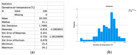
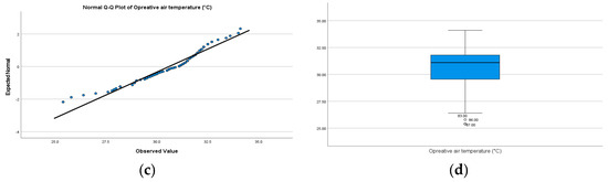
Figure 22.
(a) Skewness and kurtosis of in situ recorded operative air temperature; (b) histogram of operative air temperature; (c) normality analysis of operative air temperature; (d) whisker graph of operative air temperature.
During this monitoring period, it was observed that both the indoor and outdoor RH ranged between 57.84% and 59.17%, within the benchmark thermal comfort range (40–60%), particularly during the heatwave periods. In relation to the static ‘comfort’ range in the 2006 CIBSE Guide A, the indoor air temperatures in the living room were mainly well above the comfort range (25 °C ± 3 K) for a non-air-conditioned living room, although there were some instances of temperatures above 28 °C and below 25 °C.
In this study, it can be seen that the temperatures were significantly higher throughout the measurement and monitoring period between the 28th of July and the 2nd of September, with several instances in which the temperature was above 35 °C but never below 25 °C. Moreover, the recorded temperatures were significantly higher throughout the measurement period, with several occurrences in which the temperature was above 30 °C but never below 25 °C. The average mean indoor air temperature across 100 measured living rooms was 30.59 °C. When cross-related with the outdoor air temperature data, it was apparent that these figures correlated with the outdoor temperatures and highlighted the impact of long-term heatwaves on the overheating risk within the buildings.
5. Discussion
The data obtained from various sources highlight the positive impact of implementing air conditioning systems or incorporating natural ventilation in buildings on the IAQ in urban regions of Pakistan. Particularly during the scorching and humid months of May through September, these strategies have proven to be highly effective in creating a thermally comfortable environment for people. The key finding of this research indicates that adopting such conditioning methods can lead to a reduction of up to 25% or even less in the percentage of individuals who express dissatisfaction with their indoor conditions. This study also brings attention to the noteworthy contribution of air conditioning systems in maintaining occupant comfort and effectively removing PM2.5 particulate matter from indoor air.
5.1. Climate Change and Its Impact on Thermal Comfort
The effects of climate change can greatly influence thermal comfort, which pertains to the personal interpretation of comfort in relation to temperature and other surrounding conditions. The global rise in temperatures caused by climate change has resulted in more frequent, intense, and prolonged heat waves, especially in urban regions. These high temperatures can contribute to heat stress, dehydration, and heat-related illnesses, thereby undermining thermal comfort [81]. The changing climate is causing shifts in seasonal patterns, resulting in warmer temperatures during traditionally cooler seasons. This alteration can disturb the natural process of adjusting to temperature changes, posing difficulties in attaining thermal comfort during transitional periods. Climate change alters climatic conditions and precipitation patterns, potentially leading to shifts in climate zones [82,83]. This can disrupt the adaptation of buildings and infrastructure to local conditions, making it challenging to maintain optimal thermal comfort.
5.2. Limitations
The study focuses specifically on Lahore, which may limit the generalizability of the findings to other urban regions in Pakistan or other countries. The unique characteristics of Lahore, such as climate, building structures, and population density, may influence the effectiveness and applicability of the identified approaches and technologies. The study may involve a specific sample of buildings or households, which could introduce selection bias. For instance, if the study primarily focuses on certain types of buildings or occupants who already have access to advanced air conditioning systems, the findings may not represent the broader population accurately. While the study highlights the potential improvements in air quality through advanced air conditioning systems, it may not thoroughly explore the cost implications of adopting and maintaining such technologies. The feasibility and affordability of these systems for various segments of the population may significantly impact their widespread adoption and scalability.
5.3. Future Recommendations
Given the positive impact of air conditioning systems on IAQ and occupant comfort, it is recommended to encourage the installation and use of air conditioning systems in buildings, particularly in urban regions of Pakistan. This can help create a thermally comfortable environment for people, especially during the hot and humid months. Alongside air conditioning systems, it is important to promote the incorporation of natural ventilation strategies in buildings. Natural ventilation can complement air conditioning systems and help improve IAQ by bringing in fresh air and removing pollutants. Design guidelines and building codes can be developed to encourage the incorporation of natural ventilation features in buildings. Given the finding that air conditioning systems contribute to the effective removal of PM2.5 particulate matter from indoor air, it is recommended to monitor and control PM2.5 levels in buildings. This can be achieved through the use of air quality monitoring devices and implementing filtration systems that target PM2.5 particles. Regular maintenance and replacement of air filters should be emphasized to ensure their effectiveness.
5.4. Contribution to the Knowledge
The study contributes to the development of occupants’ adaptive thermal comfort by using both the field survey and ASHRAE Global Thermal Comfort datasets to perform the statistical analysis for an evidence-based methodological framework. In this study, some normality tests were conducted for sample sizes smaller than 100 (i.e., the Shapiro–Wilk and Kolmogorov–Smirnov tests). If these tests are significant beyond p < 0.001, these variables should be further inspected. Graphing methods were also employed for assessing normality. These graphs include histograms, normal quantile–quantile (Q–Q) plots, and box plots. Histograms should look fairly bell-shaped. Q–Q plots should follow a straight line when plotting the expected values against the observed values. Box plots show the overall interquartile range and whether extreme values exist in the variable (see the section on outliers below). If the data contain outliers, graphic displays both with and without the outliers should be examined to see how the graphs changed. If a continuous variable has serious deviations from normality, it must be addressed through transformation (log, inverse, Box–Cox, etc.), recording into an ordinal variable, or assessment for whether nonparametric analysis needs to be conducted. Regardless, researchers should run analysis both with and without outliers to see whether the pattern of results changes. Univariate and multivariate outliers are also known as extreme values and can significantly bias any parametric test. We have checked our variables for univariate outliers. SPSS identifies these values as being three times the interquartile range beyond the 25th and 75th percentile values. In the present study, multivariate outliers were tested before the primary analyses were conducted where appropriate. All continuous variables were constructed horizontally in the dataset with the following information: statistics summary table, histogram, normal Q–Q plot, box plot, and relevant notes about outliers (if applicable). The statistics summary, histogram, Q–Q plot and box plots were reviewed together to determine if variables were significantly skewed, flat or peaked. A variable that violates normality will present as being non-normal across most, if not all, of the graphs and summary information. In this study, the representative findings titled “Test of Normality” can be found that displays the results from the Kolmogorov–Smirnov and Shapiro–Wilk tests. If the sample size is smaller than 100, we highlight the variables that violated one or both of these tests. If the sample size is larger than 100, this tab can be reviewed, but reviewing these tests is not necessary. Note that if the data contain variables with outliers, then the “outliers removed” variables were tested as well. Skewness, time-of-day/kurtosis issues, indoor DEW, and data mining methods were used to resolve the issues detected in these variables before undertaking the relevant statistical analyses. The results show that 81% of recorded air temperatures were slightly above the indicated benchmarks; in line with these data, 67% of recorded RH levels were well above the suggested benchmarks. These results suggest that 90% of temperatures recorded in living room spaces were above the lower comfort threshold benchmark of 23 °C. However, in bedroom spaces, approximately 100% of the recorded temperatures were above 23 °C. Over six weeks of in situ measurements, the mean living room temperature was 27.5 °C ± 2.5 °C, and the mean bedroom temperature was 29 °C ± 4 °C. These results demonstrate that PMV can be useful in preventing overheating during summer, but improvement in the period of indoor thermal comfort was found to be significant. The mean RH for the living room spaces was 57% at ±17%, which is slightly above the indicated 40–60% benchmarking criteria.
6. Conclusions
This study aims to address the pressing concern of indoor air pollution in urban agglomeration regions of Pakistan, specifically focusing on Lahore. It emphasizes the importance of considering not only outdoor air quality but also occupants’ thermal comfort. The main objective of this investigation is to assess previous approaches, particularly the use of air conditioning systems in developed countries, to demonstrate the potential improvements in air quality that can be achieved in urban regions of Pakistan. The primary research question that was addressed was: What are the indicative associations between the PM2.5 with operative air temperature and occupants’ thermal comfort in densely built urban agglomeration regions in Pakistan?
The study examines the causes, concentrations, and impacts of various pollutants, such as particulate matter (PM2.5), carbon oxides (COx), nitrogen oxides (NOx), sulfur oxides (SOx), and volatile organic compounds (VOCs). By analyzing these factors, the research aims to provide a comprehensive understanding of the air pollution scenario specific to Lahore and similar urban regions in Pakistan. The results indicated that the average concentration of indoor pollutants in Pakistan includes particulate matter (PM) [100–250 µg/m3 for PM2.5, 200–600 µg/m3 for PM10], 1–20 ppm for carbon monoxide (CO), nitrogen oxides (NOx) [50–100 µg/m3 for NO2, 20–40 µg/m3 for NO], 20–50 µg/m3 for sulfur dioxide (SO2), and volatile organic compounds (VOCs), including 0.1–0.5 ppm for formaldehyde, 5–10 µg/m3 for benzene, and 20–30 µg/m3 for toluene. These concentrations can vary based on the source of pollution, location, and time of day.
The findings of the study highlight the significant role that air conditioning systems can play in ensuring the comfort of occupants while also aiding in the removal of PM2.5 particulate matter from indoor air. To achieve this, the study explores the use of tools such as the CLIMA tool and the ASHRAE Global Thermal Comfort Database II. These resources facilitate the assessment of and improvement in IAQ through the optimization of air conditioning systems. Specifically, certain air conditioning systems equipped with advanced features like high-efficiency particulate air (HEPA) filters, multi-stage filtration systems, and activated carbon filters are identified as highly effective in capturing and filtering out PM2.5 particles. Consequently, these systems significantly contribute to improving IAQ, ensuring healthier and safer environments for occupants. In summary, this study provides a comprehensive examination of indoor air pollution in urban regions of Pakistan, with a focus on Lahore. By highlighting the potential enhancements in air quality achievable through the adoption of advanced air conditioning systems and associated filtration technologies, the research underscores the importance of prioritizing both outdoor and IAQ for the well-being and health of urban residents.
Funding
This research received no external funding.
Acknowledgments
The first author would like to acknowledge the Sustainable Environment and Energy Systems (SEES) Graduate Program at the Middle East Technical University Northern Cyprus Campus (METU NCC) as the work presented is an outcome of an MSc degree course (SEES 586—Environmental Design and Engineering). The second author (Bertug Ozarisoy) would also like to acknowledge the School of the Built Environment and Architecture, at the London South Bank University (LSBU), London, United Kingdom.
Conflicts of Interest
The authors declare no known competing financial interests or personal relationships that could have appeared to influence the work reported in this paper.
Abbreviations
| IAQ | Indoor air quality |
| EPA | Environmental Protection Agency of Pakistan |
| WHO | World Health Organization |
| MVS | Mechanical ventilation systems |
| NVS | Natural ventilation systems |
| PAC | Portable air cleaners |
| AC | Air conditioners |
| HEPA | High-efficiency particulate air |
| UTCI | Universal Thermal Climate Index |
| PMV | Predicted mean vote |
References
- Parekh, P.P.; Khwaja, H.A.; Khan, A.R.; Naqvi, R.R.; Malik, A.; Shah, S.A.; Khan, K.; Hussain, G. Ambient air quality of two metropolitan cities of Pakistan and its health implications. Atmos. Environ. 2001, 35, 5971–5978. [Google Scholar] [CrossRef]
- Anjum, M.S.; Ali, S.M.; Imad-ud-din, M.; Subhani, M.A.; Anwar, M.N.; Nizami, A.S.; Ashraf, U.; Khokhar, M.F. An Emerged Challenge of Air Pollution and Ever-Increasing Particulate Matter in Pakistan: A Critical Review. J. Hazard. Mater. 2021, 402, 123943. [Google Scholar] [CrossRef] [PubMed]
- Barn, P.; Larson, T.; Noullett, M.; Kennedy, S.; Copes, R.; Brauer, M. Infiltration of forest fire and residential wood smoke: An evaluation of air cleaner effectiveness. J. Expo. Sci. Environ. Epidemiol. 2008, 18, 503–511. [Google Scholar] [CrossRef]
- Sharma, R.; Balasubramanian, R. Indoor human exposure to size-fractionated aerosols during the 2015 Southeast Asian smoke haze and assessment of exposure mitigation strategies. Environ. Res. Lett. 2017, 12, 114026. [Google Scholar] [CrossRef]
- Belias, E.; Licina, D. European residential ventilation: Investigating the impact on health and energy demand. Energy Build. 2024, 304, 113839. [Google Scholar] [CrossRef]
- Considine, B.; Gallagher, J.; Kumar, P.; McNabola, A. Long-term assessment of energy consumption reduction in a building ventilation system with passive particulate matter control technology in the fresh air intake. Energy Build. 2024, 309, 114067. [Google Scholar] [CrossRef]
- Zhang, X.; Wu, Y.; Shen, L.; Skitmore, M. A prototype system dynamic model for assessing the sustainability of construction projects. Int. J. Proj. Manag. 2014, 32, 66–76. [Google Scholar] [CrossRef]
- Ghauri, B.; Salam, M.; Mirza, M.I. An assessment of air quality in Karachi, Pakistan. Environ. Monit. Assess. 1994, 32, 37–45. [Google Scholar] [CrossRef]
- Colbeck, I.; Nasir, Z.A.; Ali, Z. The state of ambient air quality in Pakistan—A review. Environ. Sci. Pollut. Res. 2010, 17, 49–63. [Google Scholar] [CrossRef]
- Vahlsing, C.; Smith, K.R. Global review of national ambient air quality standards for PM10 and SO2 (24 h). Air Qual. Atmos. Health 2012, 5, 393–399. [Google Scholar] [CrossRef]
- Chow, J.C. Measurement methods to determine compliance with ambient air quality standards for suspended particles. J. Air Waste Manag. Assoc. 1995, 45, 320–382. [Google Scholar] [CrossRef]
- Özden, Ö.; Döǧeroǧlu, T.; Kara, S. Assessment of ambient air quality in Eskişehir, Turkey. Environ. Int. 2008, 34, 678–687. [Google Scholar] [CrossRef] [PubMed]
- Anwar, M.N.; Shabbir, M.; Tahir, E.; Iftikhar, M.; Saif, H.; Tahir, A.; Murtaza, M.A.; Khokhar, M.F.; Rehan, M.; Aghbashlo, M.; et al. Emerging challenges of air pollution and particulate matter in China, India, and Pakistan and mitigating solutions. J. Hazard. Mater. 2021, 416, 125851. [Google Scholar] [CrossRef] [PubMed]
- IQ Air. World Air Quality Report. 2022. Available online: https://www.iqair.com/newsroom/world-air-quality-report-press-release-2022 (accessed on 16 June 2024).
- Jones, A. Indoor air quality and health. Atmos. Environ. 1999, 33, 4535–4564. [Google Scholar] [CrossRef]
- Gil-Baez, M.; Lizana, J.; Becerra Villanueva, J.A.; Molina-Huelva, M.; Serrano-Jimenez, A.; Chacartegui, R. Natural ventilation in classrooms for healthy schools in the COVID era in Mediterranean climate. Build. Environ. 2021, 206, 108345. [Google Scholar] [CrossRef]
- Ahmed, T.; Kumar, P.; Mottet, L. Natural ventilation in warm climates: The challenges of thermal comfort, heatwave resilience and indoor air quality. Renew. Sustain. Energy Rev. 2021, 138, 110669. [Google Scholar] [CrossRef]
- Tran, P.T.M.; Adam, M.G.; Balasubramanian, R. Mitigation of indoor human exposure to airborne particles of outdoor origin in an urban environment during haze and non-haze periods. J. Hazard. Mater. 2021, 403, 123555. [Google Scholar] [CrossRef] [PubMed]
- Ramalho, O.; Wyart, G.; Mandin, C.; Blondeau, P.; Cabanes, P.A.; Leclerc, N.; Mullot, J.U.; Boulanger, G.; Redaelli, M. Association of carbon dioxide with indoor air pollutants and exceedance of health guideline values. Build. Environ. 2015, 93, 115–124. [Google Scholar] [CrossRef]
- Wei, W.; Ramalho, O.; Mandin, C. Indoor air quality requirements in green building certifications. Build. Environ. 2015, 92, 10–19. [Google Scholar] [CrossRef]
- Wei, G.; Yu, X.; Fang, L.; Wang, Q.; Tanaka, T.; Amano, K.; Yang, X. A review and comparison of the indoor air quality requirements in selected building standards and certifications. Build. Environ. 2022, 226, 109709. [Google Scholar] [CrossRef]
- Tran, P.T.M.; Adam, M.G.; Tham, K.W.; Schiavon, S.; Pantelic, J.; Linden, P.F.; Sofianopoulou, E.; Sekhar, S.C.; Cheong, D.K.W.; Balasubramanian, R. Assessment and mitigation of personal exposure to particulate air pollution in cities: An exploratory study. Sustain. Cities Soc. 2021, 72, 103052. [Google Scholar] [CrossRef]
- Kalimeri, K.K.; Saraga, D.E.; Lazaridis, V.D.; Legkas, N.A.; Missia, D.A.; Tolis, E.I.; Bartzis, J.G. Indoor air quality investigation of the school environment and estimated health risks: Two-season measurements in primary schools in Kozani, Greece. Atmos. Pollut. Res. 2016, 7, 1128–1142. [Google Scholar] [CrossRef]
- Chiara Pietrogrande, M.; Casari, L.; Demaria, G.; Russo, M. Indoor Air Quality in Domestic Environments during Periods Close to Italian COVID-19 Lockdown. Int. J. Environ. Res. Public Health Artic. Res. Public Health 2021, 18, 4060. [Google Scholar] [CrossRef] [PubMed]
- Becerra, J.A.; Lizana, J.; Gil, M.; Barrios-Padura, A.; Blondeau, P.; Chacartegui, R. Identification of potential indoor air pollutants in schools. J. Clean. Prod. 2020, 242, 118420. [Google Scholar] [CrossRef]
- Fakhri, Y.; Akhlaghi, M.; Daraei, H.; Hedarinejad, Z.; Bahreini, A.; Mahmudiono, T.; Mousavi Khaneghah, A. The concentration of potentially toxic elements (zinc, iron, manganese) bound PM2.5 in the indoor air of urban schools: A global systematic review and meta-analysis. Air Qual. Atmos. Health 2023, 16, 77–84. [Google Scholar] [CrossRef]
- Abdel-Salam, M.M.M. Investigation of PM2.5 and carbon dioxide levels in urban homes. J. Air Waste Manag. Assoc. 2015, 65, 930–936. [Google Scholar] [CrossRef]
- Abdel-Salam, M.M.M. Seasonal variation in indoor concentrations of air pollutants in residential buildings. J. Air Waste Manag. Assoc. 2021, 71, 761–777. [Google Scholar] [CrossRef]
- Karuppasamy, M.B.; Natesan, U.; Karuppannan, S.; Chandrasekaran, L.N.; Hussain, S.; Almohamad, H.; Al Dughairi, A.A.; Al-Mutiry, M.; Alkayyadi, I.; Abdo, H.G. Multivariate Urban Air Quality Assessment of Indoor and Outdoor Environments at Chennai Metropolis in South India. Atmosphere 2022, 13, 1627. [Google Scholar] [CrossRef]
- Baloch, R.M.; Maesano, C.N.; Christoffersen, J.; Banerjee, S.; Gabriel, M.; Csobod, É.; de Oliveira Fernandes, E.; Annesi-Maesano, I.; Szuppinger, P.; Prokai, R.; et al. Indoor air pollution, physical and comfort parameters related to schoolchildren’s health: Data from the European SINPHONIE study. Sci. Total Environ. 2020, 739, 139870. [Google Scholar] [CrossRef]
- Godwin, C.; Batterman, S. Indoor air quality in Michigan schools. Indoor Air 2007, 17, 109–121. [Google Scholar] [CrossRef]
- Szabados, M.; Csákó, Z.; Kotlík, B.; Kazmarová, H.; Kozajda, A.; Jutraz, A.; Kukec, A.; Otorepec, P.; Dongiovanni, A.; Di Maggio, A.; et al. Indoor air quality and the associated health risk in primary school buildings in Central—The InAirQ study. Indoor Air 2021, 31, 989–1003. [Google Scholar] [CrossRef] [PubMed]
- Balasubramanian, R.; Sheng, S.L. Characteristics of indoor aerosols in residential homes in urban locations: A case study in Singapore. J. Air Waste Manag. Assoc. 2007, 57, 981–990. [Google Scholar] [CrossRef] [PubMed]
- An, Y.; Xia, T.; You, R.; Lai, D.; Liu, J.; Chen, C. A reinforcement learning approach for control of window behavior to reduce indoor PM2.5 concentrations in naturally ventilated buildings. Build. Environ. 2021, 200, 107978. [Google Scholar] [CrossRef]
- Student Lesson. Available online: https://studentlesson.com/air-conditioning-system-definition-functions-components-types/#:~:text=An%20air%20conditioning%20system%20is,for%20human%20and%20other%20animals (accessed on 9 May 2023).
- Yu, B.F.; Hu, Z.B.; Liu, M.; Yang, H.L.; Kong, Q.X.; Liu, Y.H. Review of research on air-conditioning systems and indoor air quality control for human health. Int. J. Refrig. 2009, 32, 3–20. [Google Scholar] [CrossRef]
- LAC Temperature Control. Available online: https://lacltd.uk.com/7-benefits-of-air-conditioning-in-the-home (accessed on 14 May 2023).
- Linquip Technews. Available online: https://www.linquip.com/blog/advantages-of-air-conditioner/ (accessed on 14 May 2023).
- Berkeys Plumbing. A/C. Electrical. Available online: https://www.berkeys.com/2016/12/22/advantage-disadvantage-air-conditioner/ (accessed on 14 May 2023).
- Comfy Home Heating Cooling. Available online: https://www.comfyhome.com.au/pros-cons-of-air-conditioner/ (accessed on 14 May 2023).
- Kek, H.Y.; Mohd Saupi, S.B.; Tan, H.; Dzarfan Othman, M.H.; Nyakuma, B.B.; Goh, P.S.; Hamood Altowayti, W.A.; Qaid, A.; Abdul Wahab, N.H.; Lee, C.H.; et al. Ventilation Strategies for Mitigating Airborne Infection in Healthcare Facilities: A Review and Bibliometric Analysis (1993 to 2022). Energy Build. 2023, 295, 113323. [Google Scholar] [CrossRef]
- EPA United States Environmental Protection Agency. Available online: https://www.epa.gov/indoor-air-quality-iaq/what-hepa-filter (accessed on 19 May 2023).
- Atmostemp Heating, Air Conditioning Plumbing|A Service Experts Company. Available online: https://www.atmostempheating.com/blog/can-you-install-hepa-filters-in-your-hvac-system-in-voorhees#:~:text=There%20are%20a%20few%20different,3%2 (accessed on 20 May 2023).
- Protect COVID-19 National Core Study. Available online: https://sites.manchester.ac.uk/covid19-national-project/2023/01/09/how-we-know-that-hepa-filter-based-air-cleaners-are-likely-to-be-beneficial-for-reducing-transmission-of-respirat (accessed on 20 May 2023).
- Solberg, S.; Controlling Critical Environments with HEPA-Filtered Air-Conditioning. Dantherm Group Climate Solution. 2023. Available online: https://www.danthermgroup.com/en-gb/dantherm/controlling-critical-environments-with-hepa-filtered-air-conditioning (accessed on 16 June 2024).
- Freudenberg Innovating Together. Available online: https://www.freudenberg-filter.com/en/ (accessed on 20 May 2023).
- Freudenberg. Available online: https://web.archive.org/web/20231211084951/https://www.freudenberg-filter.com/en/filtration-know-how/protection-against-viruses/industrial-filtration/ (accessed on 20 May 2023).
- Sanalife. Available online: https://www.sanalifewellness.com/technologies/multi-stage-air-filtration (accessed on 20 May 2023).
- HVAC Training Shop. Available online: https://hvactrainingshop.com/activated-carbon-air-filters/ (accessed on 20 May 2023).
- HaoAirTech. Available online: http://www.haoairtech.com/products/pleated-active-carbon-filter/ (accessed on 20 May 2023).
- Hassan, H.; Mishra, A.K.; Wemken, N.; O’Dea, P.; Cowie, H.; McIntyre, B.; Coggins, A.M. Deep energy renovations’ impact on indoor air quality and thermal comfort of residential dwellings in Ireland—ARDEN project. Build. Environ. 2024, 259, 111637. [Google Scholar] [CrossRef]
- Sha, X.; Ma, Z.; Sethuvenkatraman, S.; Li, W. A novel rule mining method for knowledge discovery of relationships among indoor air quality, HVAC operation and occupants’ activities. Build. Environ. 2024, 260, 111670. [Google Scholar] [CrossRef]
- Takebayashi, H. Effects of air temperature, humidity, and wind velocity distribution on indoor cooling load and outdoor human thermal environment at urban scale. Energy Build. 2022, 257, 111792. [Google Scholar] [CrossRef]
- Jara-Baeza, F.; Rajagopalan, P.; Andamon, M.M. A holistic assessment of indoor environmental quality perception in Australian high-rise social housing. Energy Build. 2023, 284, 112859. [Google Scholar] [CrossRef]
- Belias, E.; Licina, D. Influence of outdoor air pollution on European residential ventilative cooling potential. Energy Build. 2023, 289, 113044. [Google Scholar] [CrossRef]
- An, Y.; Chen, C. Energy-efficient control of indoor PM2.5 and thermal comfort in a real room using deep reinforcement learning. Energy Build. 2023, 295, 113340. [Google Scholar] [CrossRef]
- Colclough, S.; Salaris, C. Quantifying overheating in nZEB Irish residential buildings. An analysis of recorded interior temperatures of Irish newbuild and retrofit residential buildings against CIBSE, Passive House and WHO overheating criteria and recorded occupant satisfaction. Energy Build. 2024, 303, 113571. [Google Scholar] [CrossRef]
- Arriazu-Ramos, A.; Ruiz, G.R.; Izquierdo, J.J.P.; Gutiérrez, A.S.O.; Monge-Barrio, A. From urban microclimate to indoor overheating: Analysis of residential typologies during typical climate series and extreme warm summer. Energy Build. 2023, 299, 113620. [Google Scholar] [CrossRef]
- Berneiser, J.; Auerswald, S.; Maier, D.; Gölz, S.; Carbonare, N.; Pflug, T. Feeling the breeze? Ventilation practices and occupant requirements for mechanical ventilation in residential buildings. Energy Build. 2024, 302, 113702. [Google Scholar] [CrossRef]
- CBE Center for the Built Environment. Low-Energy Occupant-Responsive HVAC Controls and Systems. 2023. Available online: https://cbe.berkeley.edu/research/low-energy-occupant-responsive-hvac/ (accessed on 16 June 2024).
- CBE Center for the Built Environment. Low-Cost MEMS-Based Ultrasonic Airflow Sensors for Rooms and HVAC Systems. 2023. Available online: https://cbe.berkeley.edu/research/low-cost-mems-airflow-sensors-rooms-and-hvac/ (accessed on 16 June 2024).
- World Maps of Köppen-Geiger Climate Classification. Available online: https://koeppen-geiger.vu-wien.ac.at/present.htm (accessed on 12 June 2023).
- Google Earth Pro. Available online: https://earth.google.com/web/@31.5203696,74.3587473,64524.36147026a,0d,35y,-0h,0t,0r (accessed on 15 May 2023).
- Draw.io. Available online: https://www.drawio.com/ (accessed on 12 May 2023).
- Betti, G.; Tartarini, F.; Nguyen, C.; Schiavon, S. CBE Clima Tool: A free and open-source web application for climate analysis tailored to sustainable building design. arXiv 2022, arXiv:2212.04609. [Google Scholar] [CrossRef]
- Földváry Ličina, V.; Cheung, T.; Zhang, H.; de Dear, R.; Parkinson, T.; Arens, E.; Chun, C.; Schiavon, S.; Luo, M.; Brager, G.; et al. Development of the ASHRAE Global Thermal Comfort Database II. Build. Environ. 2018, 142, 502–512. [Google Scholar] [CrossRef]
- CBE Clima Tool. Available online: https://clima.cbe.berkeley.edu/ (accessed on 24 May 2023).
- Ozarisoy, B. Supplementary data for Assessing the Domestic Energy Use and Thermal Comfort of Occupants in a Post-war Social Housing Development Estate in Famagusta, Northern Cyprus. University of East London. 2022. Available online: https://repository.uel.ac.uk/item/8q774 (accessed on 12 June 2023).
- Ozarisoy, B.; Altan, H. Regression forecasting of ‘neutral’ adaptive thermal comfort: A field study investigation in the south-eastern Mediterranean climate of Cyprus. Build. Environ. 2021, 202, 108013. [Google Scholar] [CrossRef]
- Vadoudi, K.; Marinhas, S. Development of Psychrometric diagram for the energy efficiency of Air Handling Units. AIVC Publications. 2019. Available online: https://www.aivc.org/resource/development-psychrometric-diagram-energy-efficiency-air-handling-units (accessed on 16 June 2024).
- Jiang, Y.; Chen, Q. Study of natural ventilation in buildings by large eddy simulation. J. Wind. Eng. Ind. Aerodyn. 2001, 89, 1155–1178. [Google Scholar] [CrossRef]
- Li, Y.; Delsante, A.; Symons, J. Prediction of natural ventilation in buildings with large openings. Build. Environ. 2000, 35, 191–206. [Google Scholar] [CrossRef]
- Bröde, P.; Fiala, D.; Błażejczyk, K.; Holmér, I.; Jendritzky, G.; Kampmann, B.; Tinz, B.; Havenith, G. Deriving the operational procedure for the Universal Thermal Climate Index (UTCI). Int. J. Biometeorol. 2012, 56, 481–494. [Google Scholar] [CrossRef]
- Błazejczyk, K.; Broede, P.; Fiala, D.; Havenith, G.; Holmér, I.; Jendritzky, G.; Kampmann, B.; Kunert, A. Principles of the new universal thermal climate index (UTCI) and its application to bioclimatic research in European scale. Misc. Geogr. 2010, 14, 91–102. [Google Scholar] [CrossRef]
- ASHRAE Global Thermal Comfort Database II Visualization. Available online: https://cbe-berkeley.shinyapps.io/comfortdatabase/ (accessed on 28 May 2023).
- Hubert, M.; Vandervieren, E. An adjusted boxplot for skewed distributions. Comput. Stat. Data Anal. 2008, 52, 5186–5201. [Google Scholar] [CrossRef]
- Cheung, T.; Schiavon, S.; Parkinson, T.; Li, P.; Brager, G. Analysis of the accuracy on PMV–PPD model using the ASHRAE Global Thermal Comfort Database II. Build. Environ. 2019, 153, 205–217. [Google Scholar] [CrossRef]
- Carlucci, S.; Erba, S.; Pagliano, L.; de Dear, R. ASHRAE Likelihood of Dissatisfaction: A new right-here and right-now thermal comfort index for assessing the Likelihood of dissatisfaction according to the ASHRAE adaptive comfort model. Energy Build. 2021, 250, 111286. [Google Scholar] [CrossRef]
- Zhang, S.; Yao, R.; Du, C.; Essah, E.; Li, B. Analysis of outlier detection rules based on the ASHRAE global thermal comfort database. Build. Environ. 2023, 234, 110155. [Google Scholar] [CrossRef]
- Rupp, R.F.; Parkinson, T.; Kim, J.; Toftum, J.; de Dear, R. The impact of occupant’s thermal sensitivity on adaptive thermal comfort model. Build. Environ. 2022, 207, 108517. [Google Scholar] [CrossRef]
- Rawal, R.; Shukla, Y.; Vardhan, V.; Asrani, S.; Schweiker, M.; de Dear, R.; Garg, V.; Mathur, J.; Prakash, S.; Diddi, S.; et al. Adaptive thermal comfort model based on field studies in five climate zones across India. Build. Environ. 2022, 219, 109187. [Google Scholar] [CrossRef]
- Parkinson, T.; de Dear, R.; Brager, G. Nudging the adaptive thermal comfort model. Energy Build. 2020, 206, 109559. [Google Scholar] [CrossRef]
- Ji, W.; Zhu, Y.; Cao, B. Development of the Predicted Thermal Sensation (PTS) model using the ASHRAE Global Thermal Comfort Database. Energy Build. 2020, 211, 109780. [Google Scholar] [CrossRef]

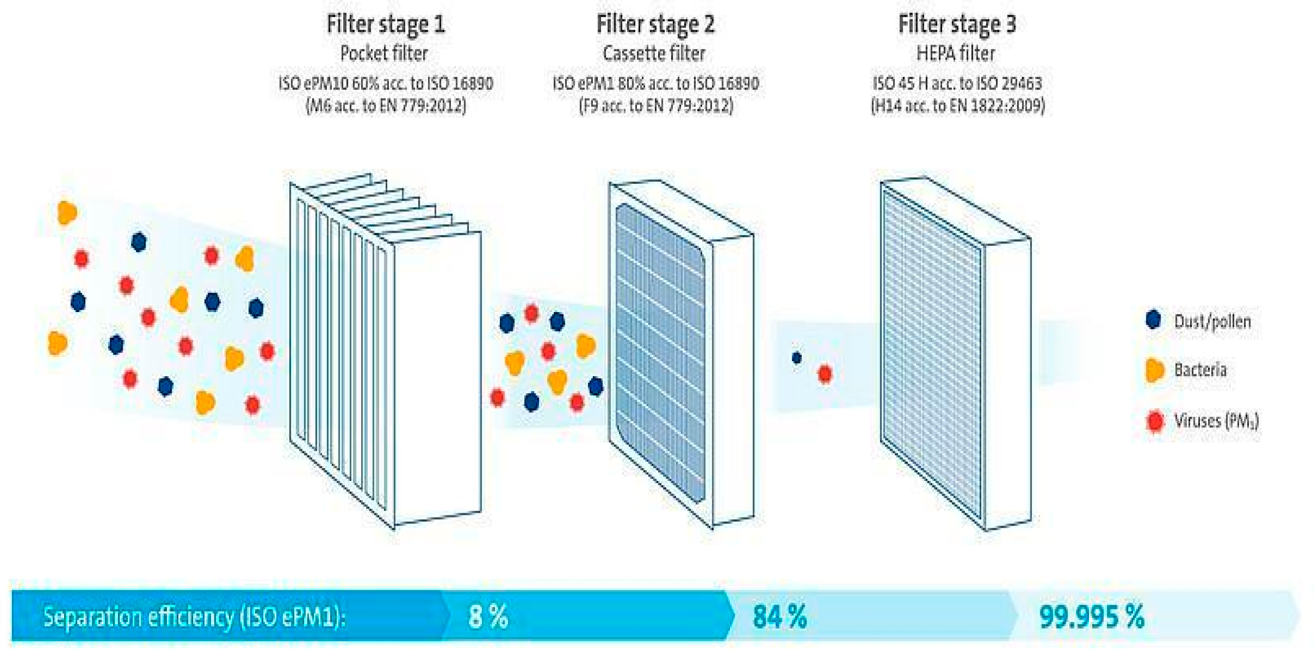
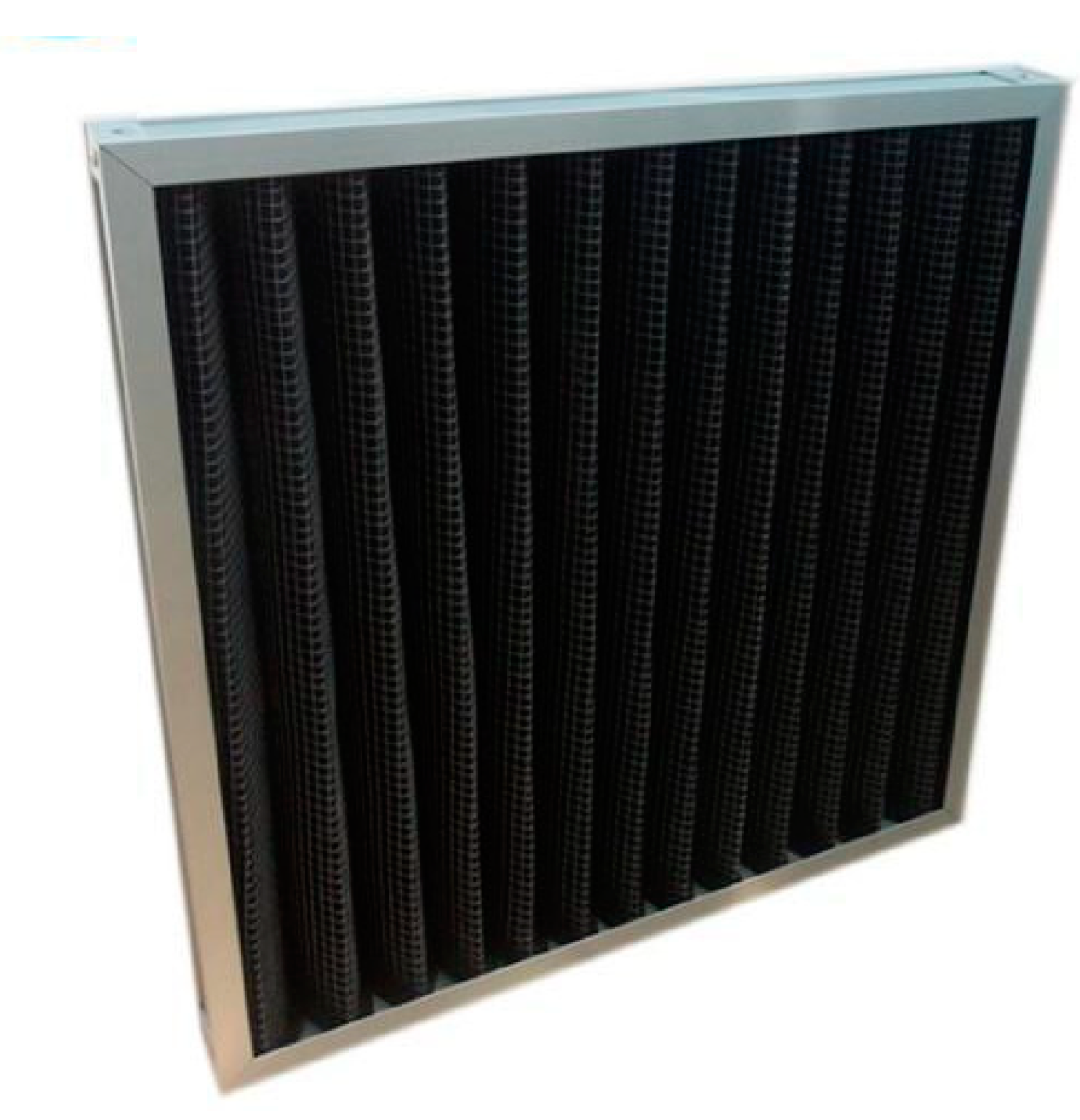

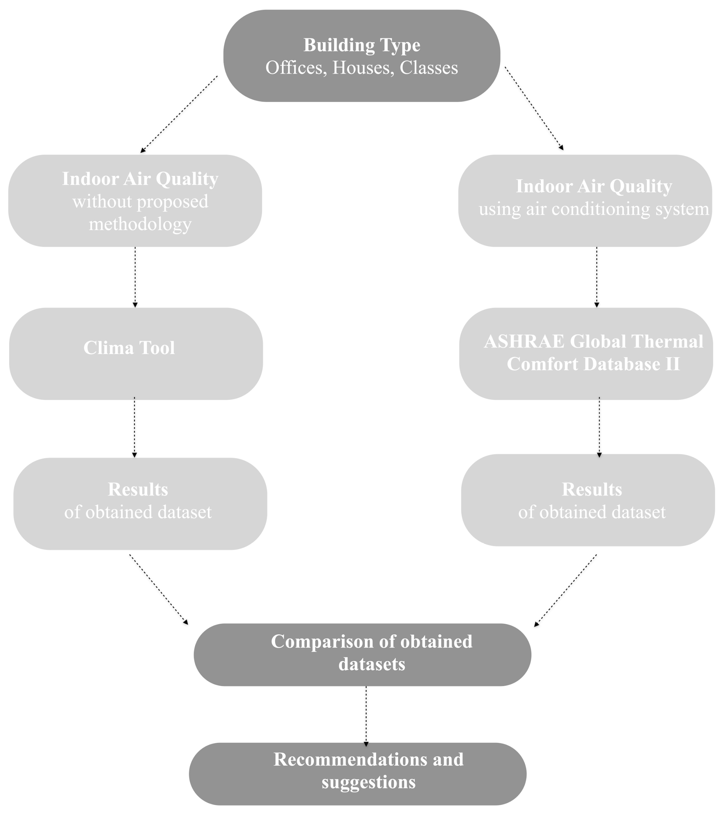
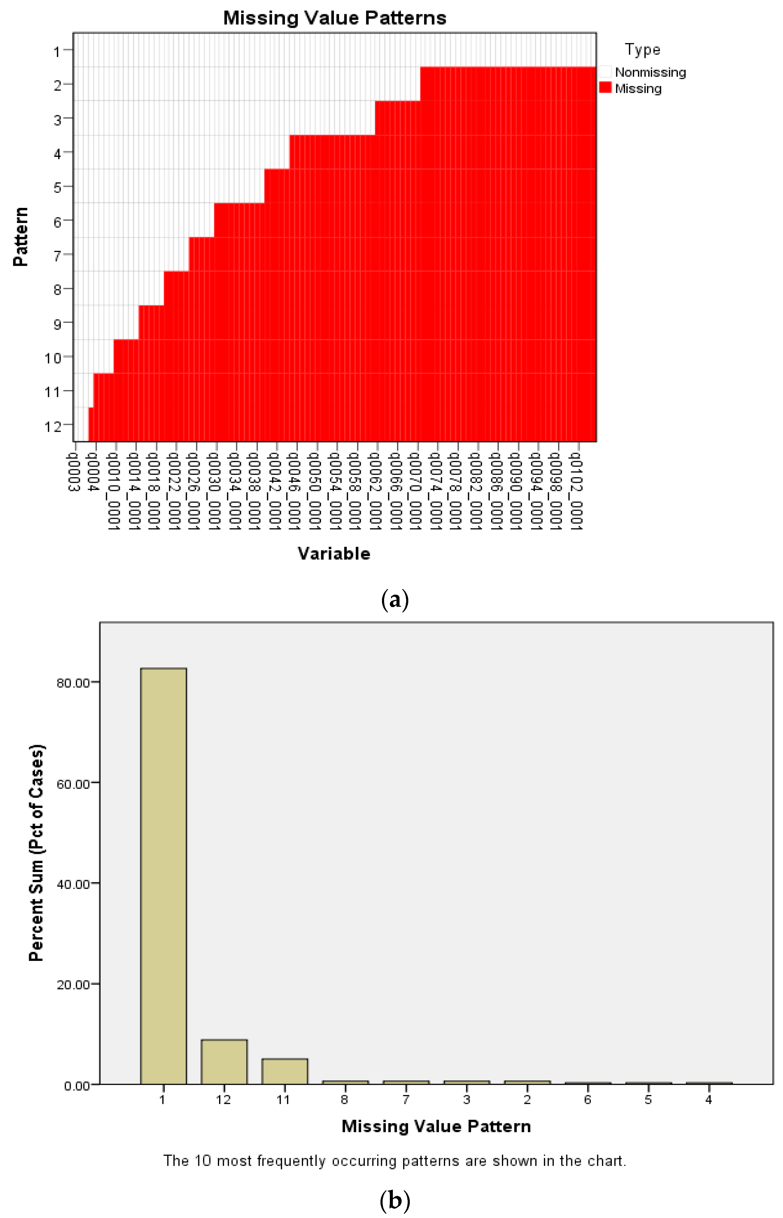

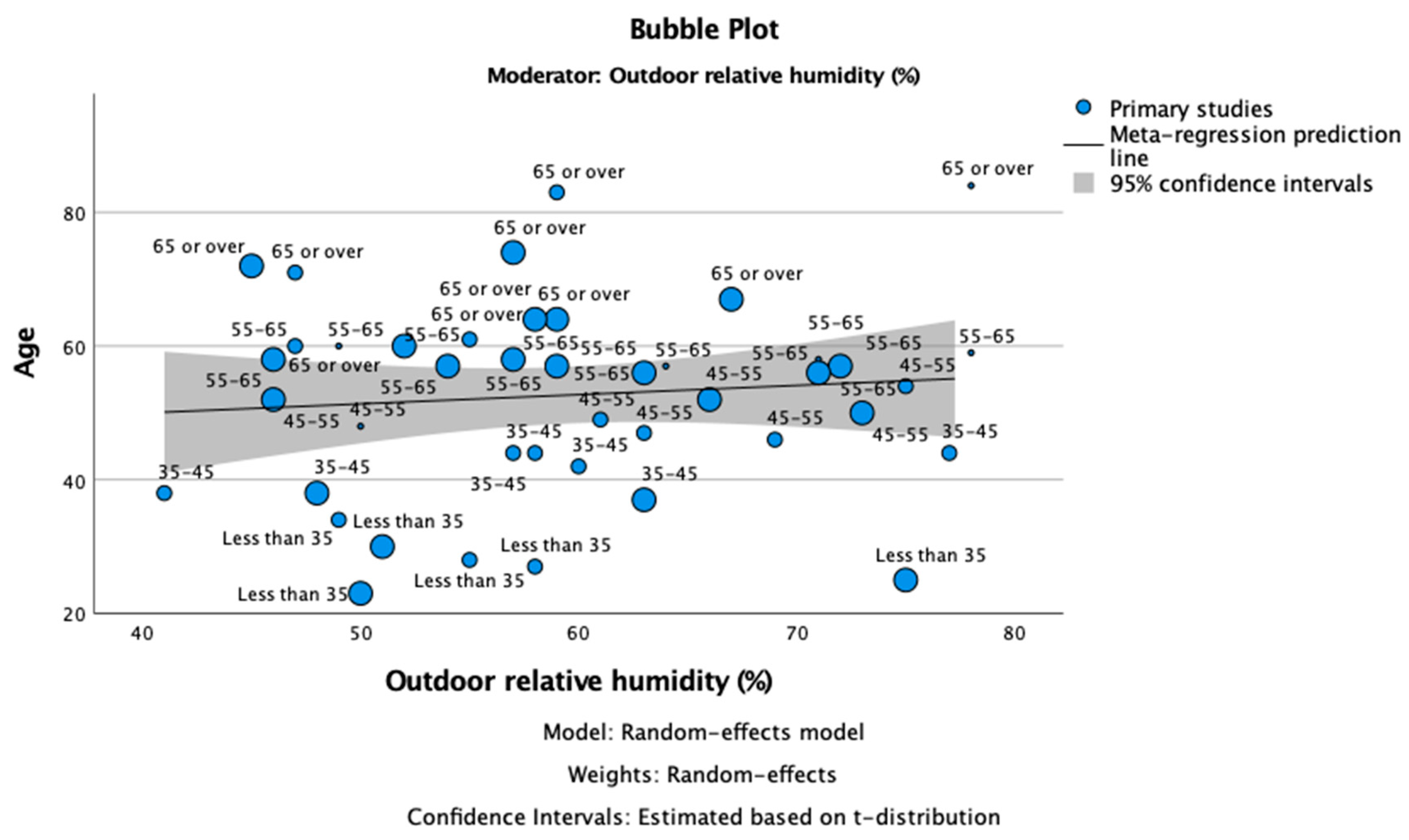
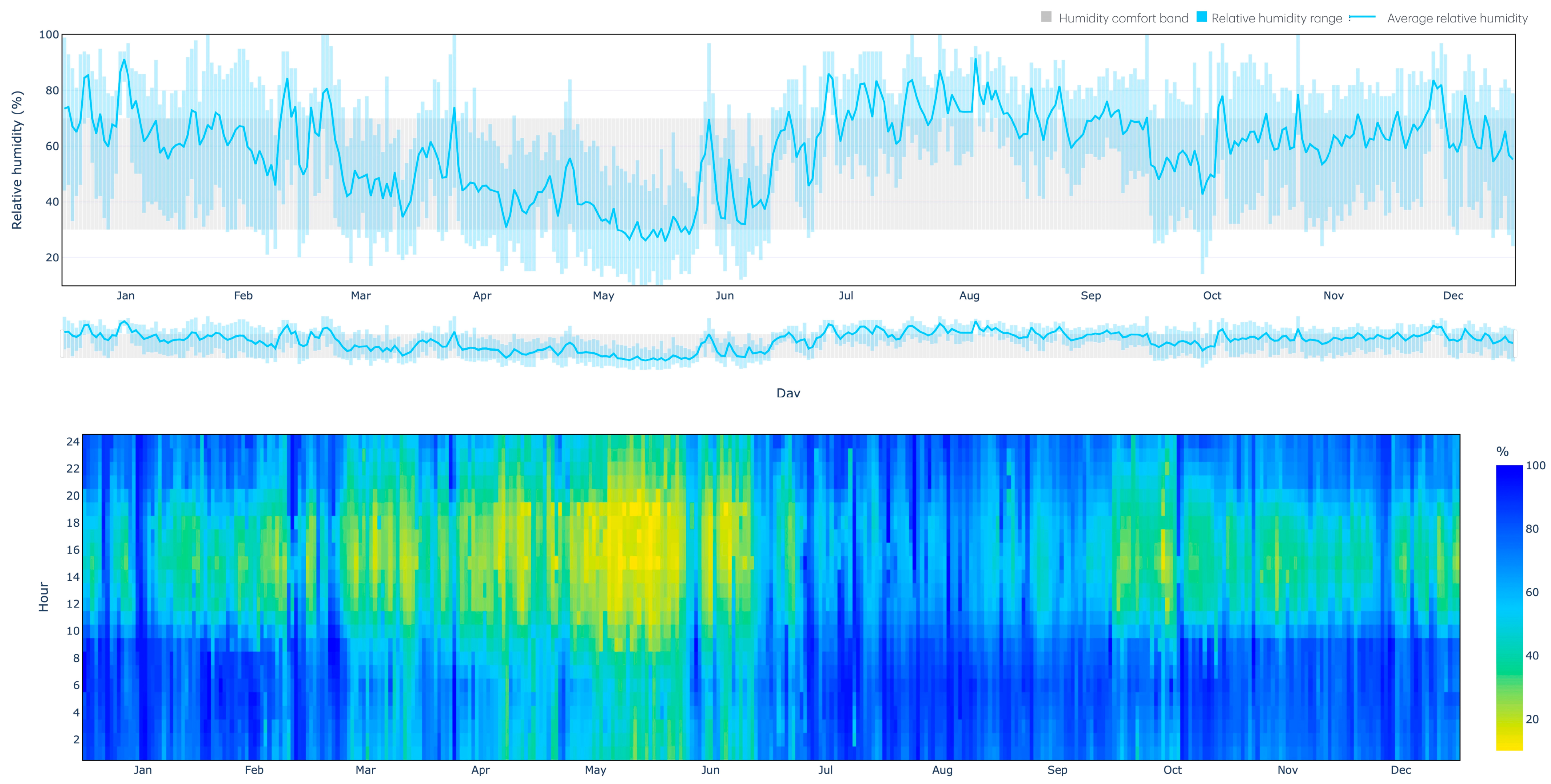
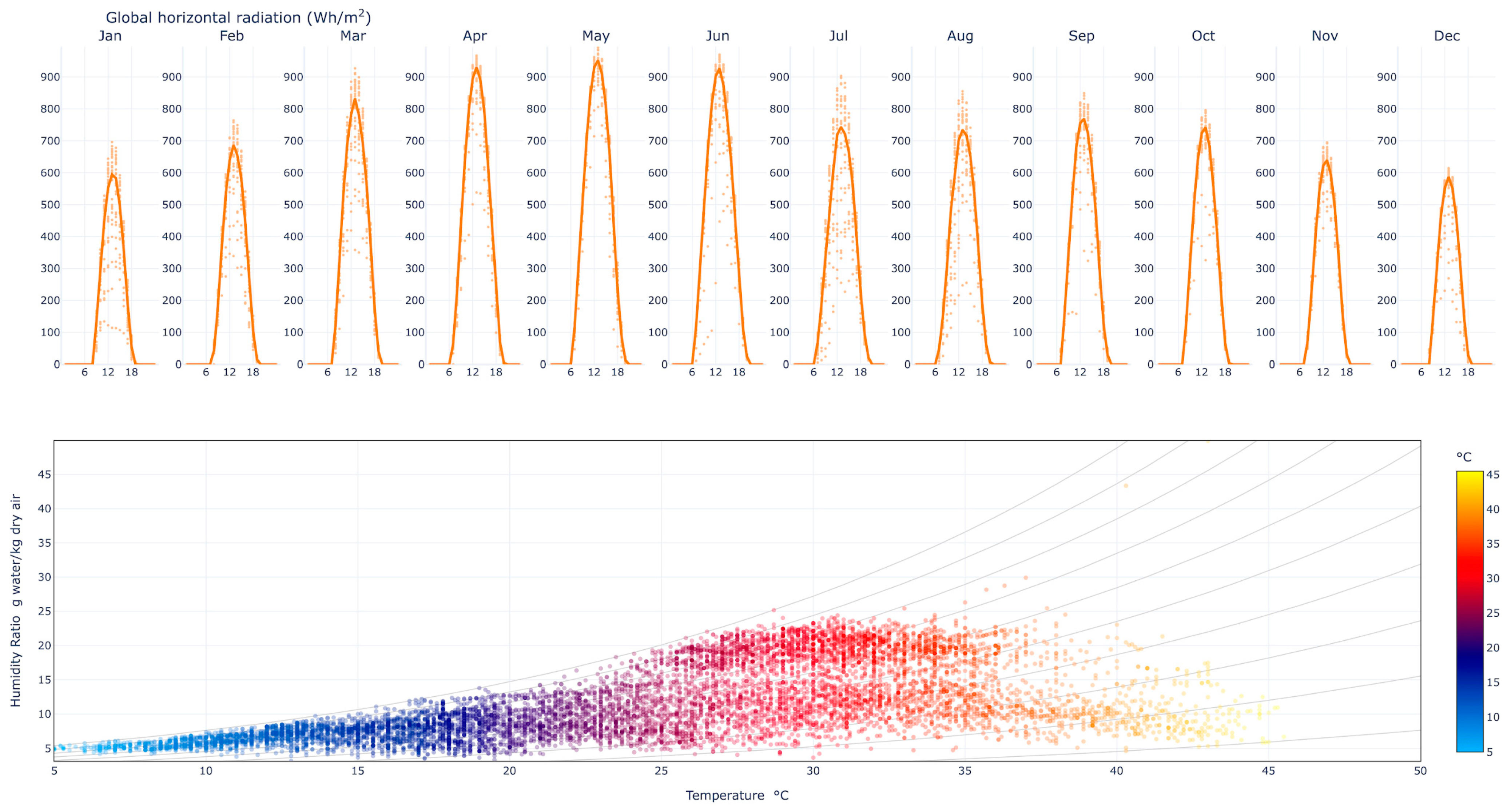
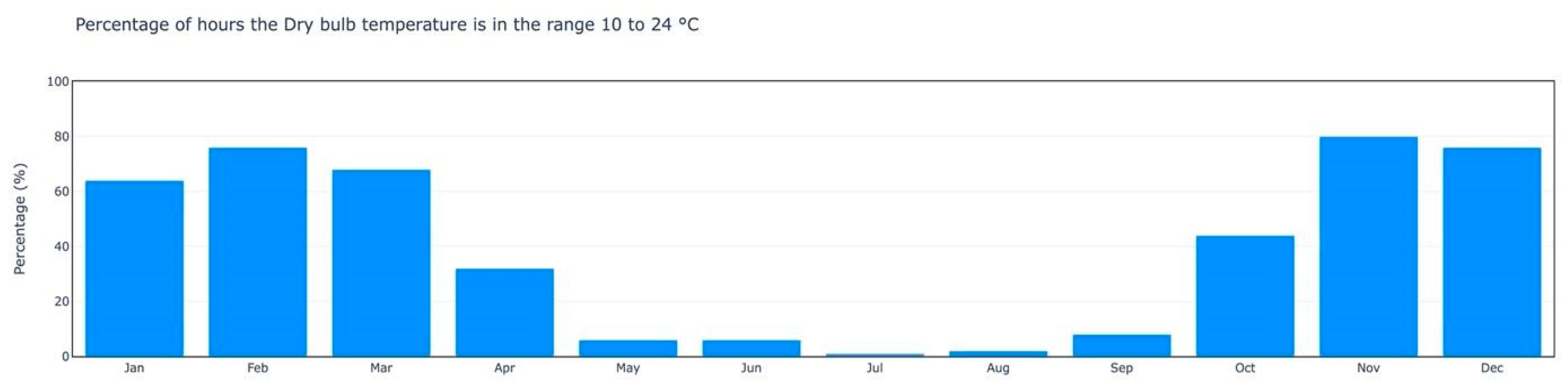
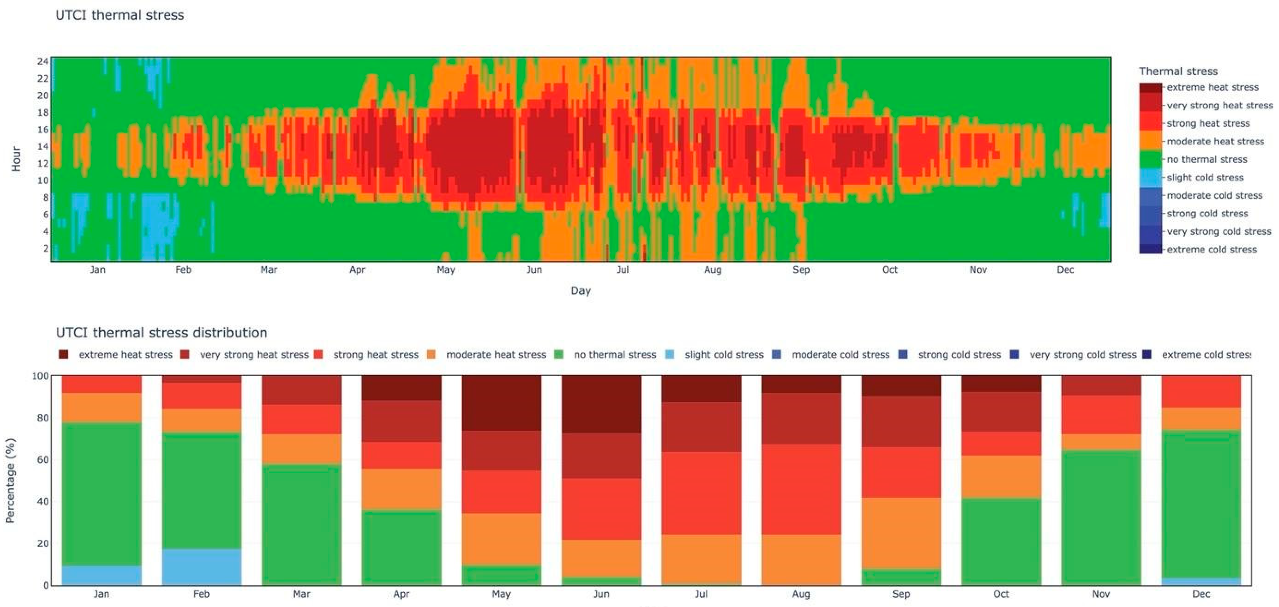
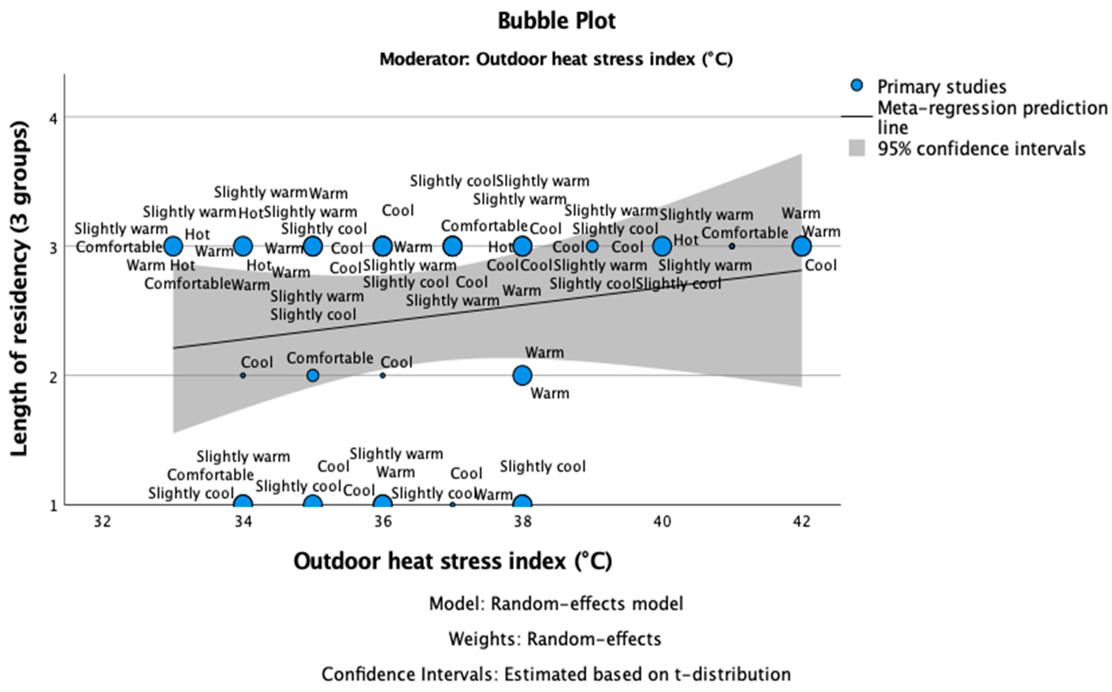
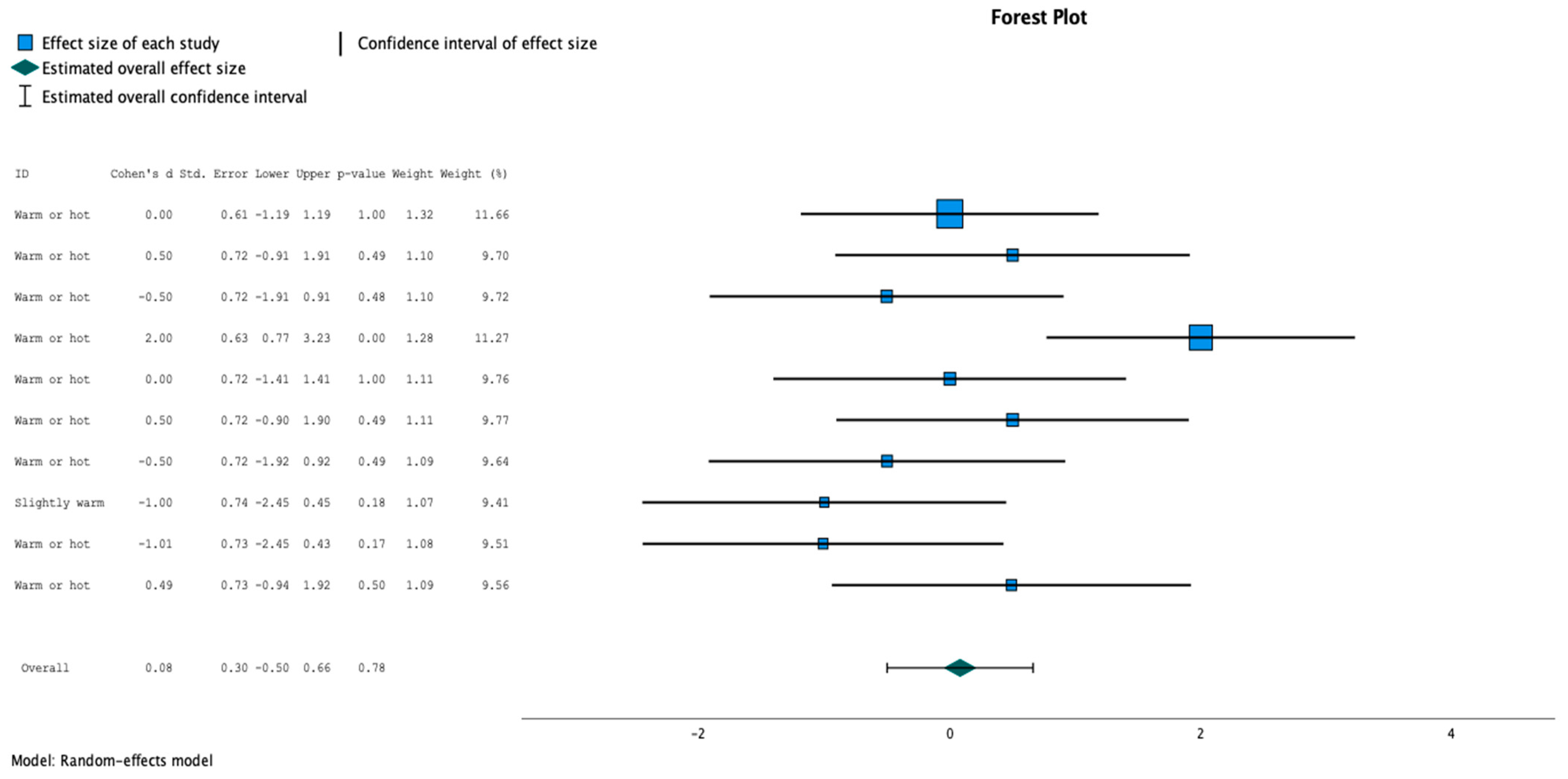
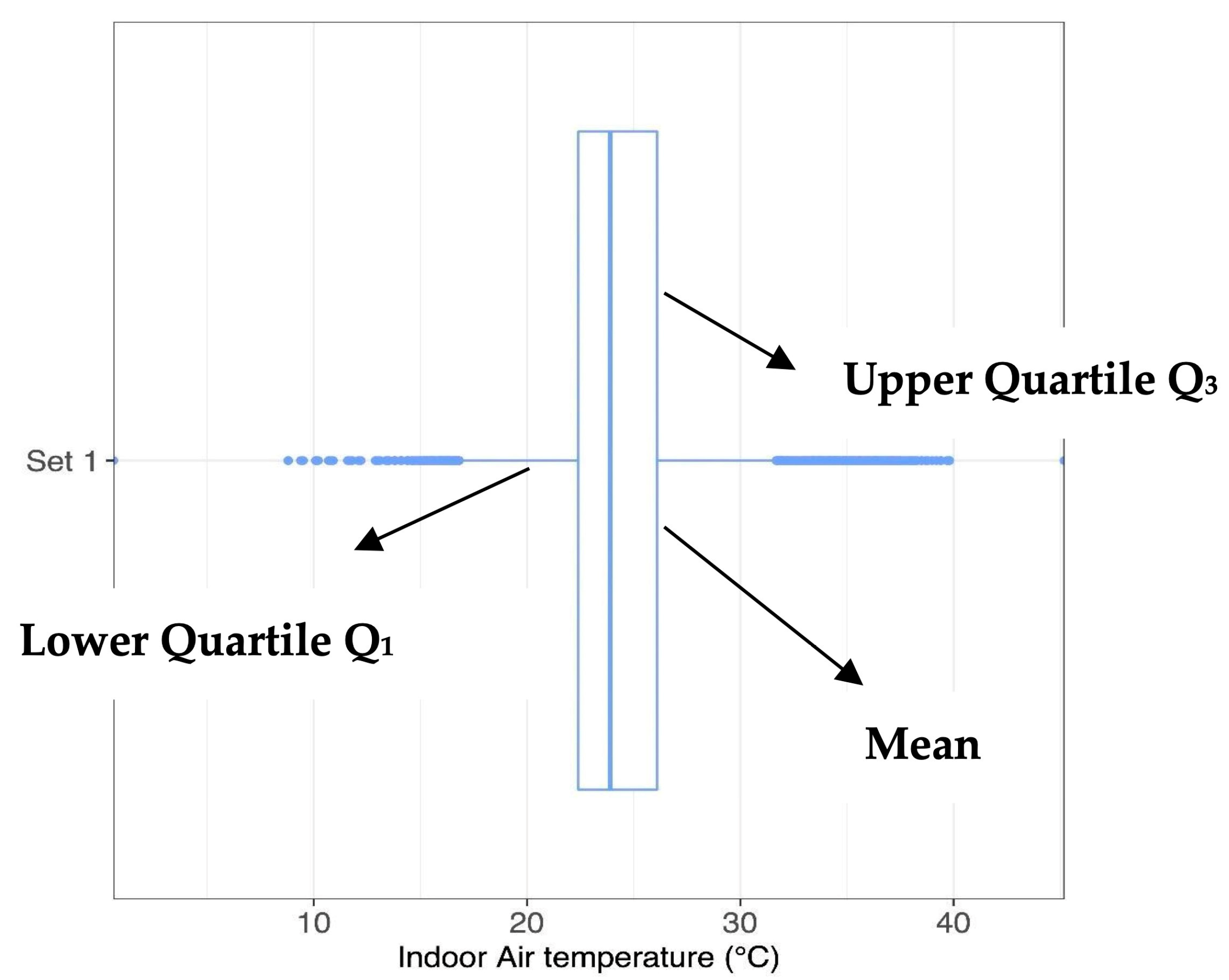
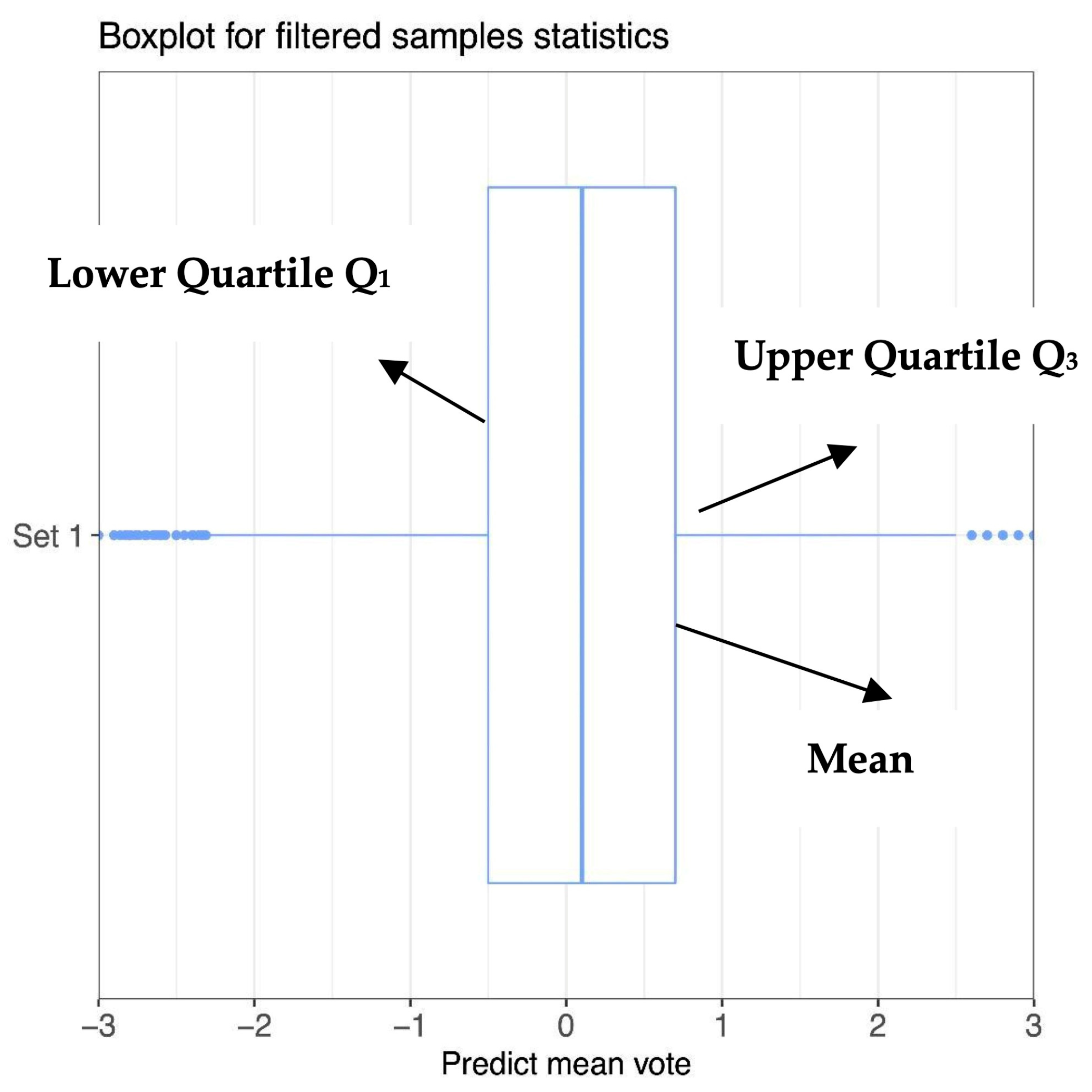

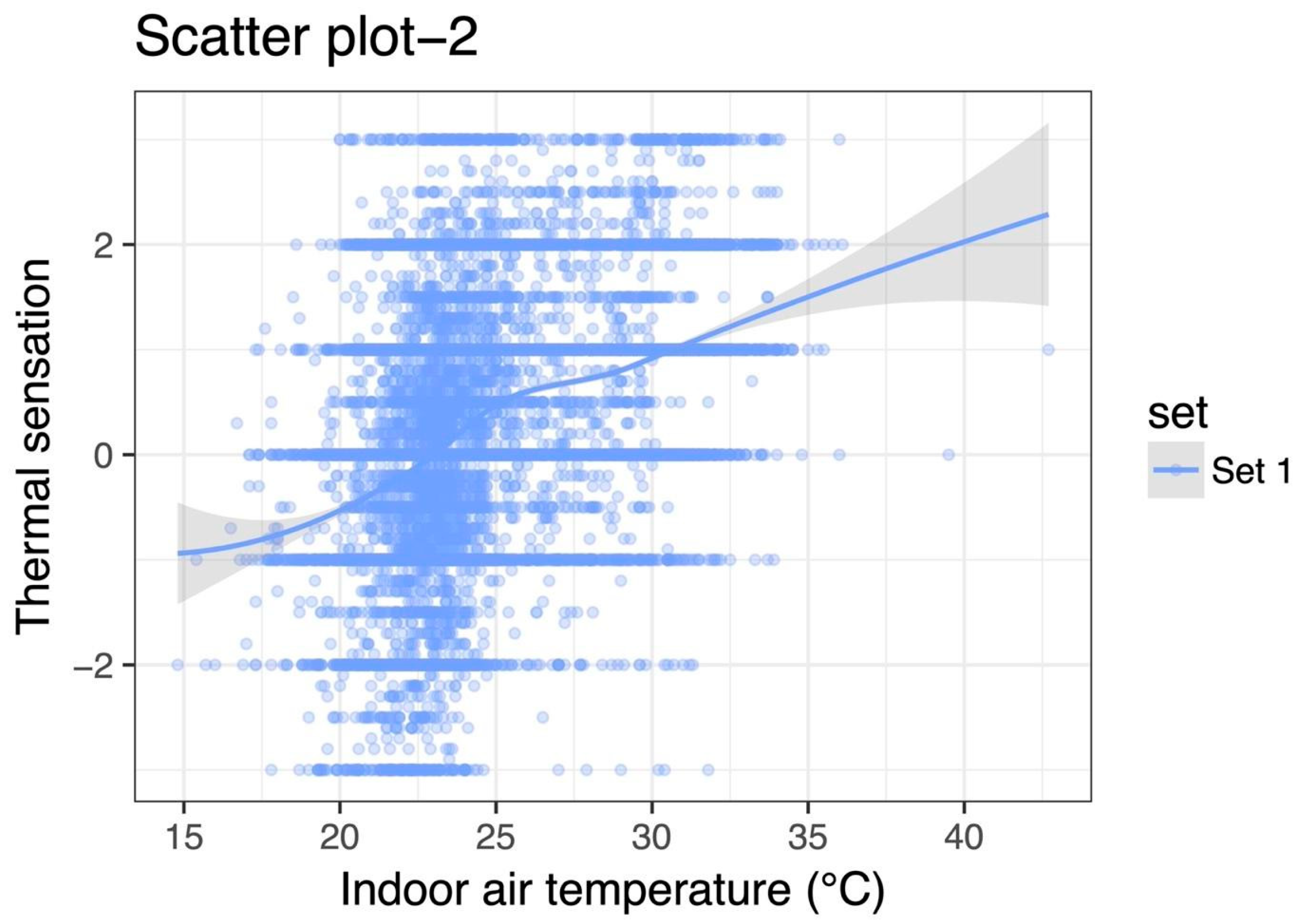
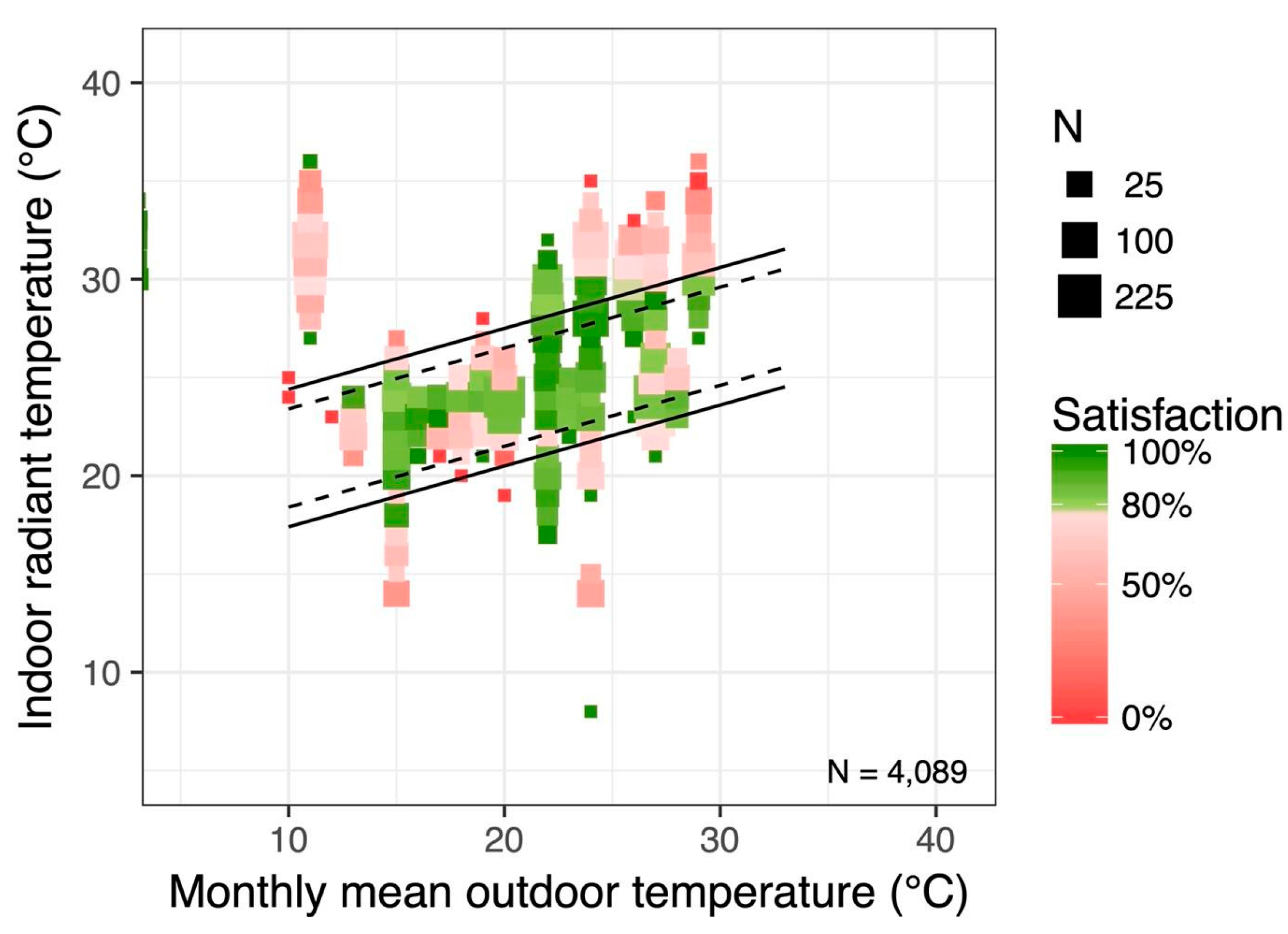
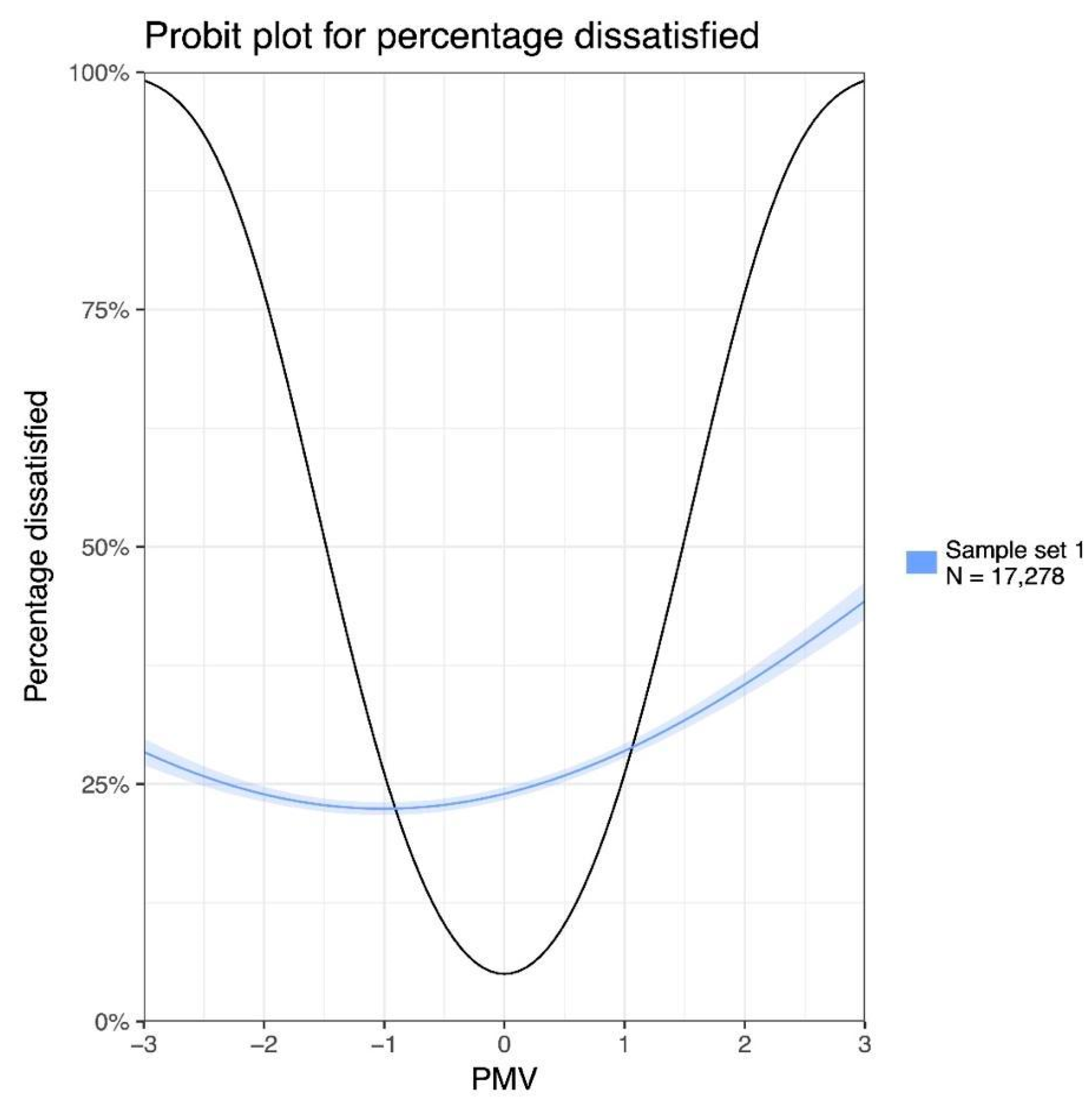
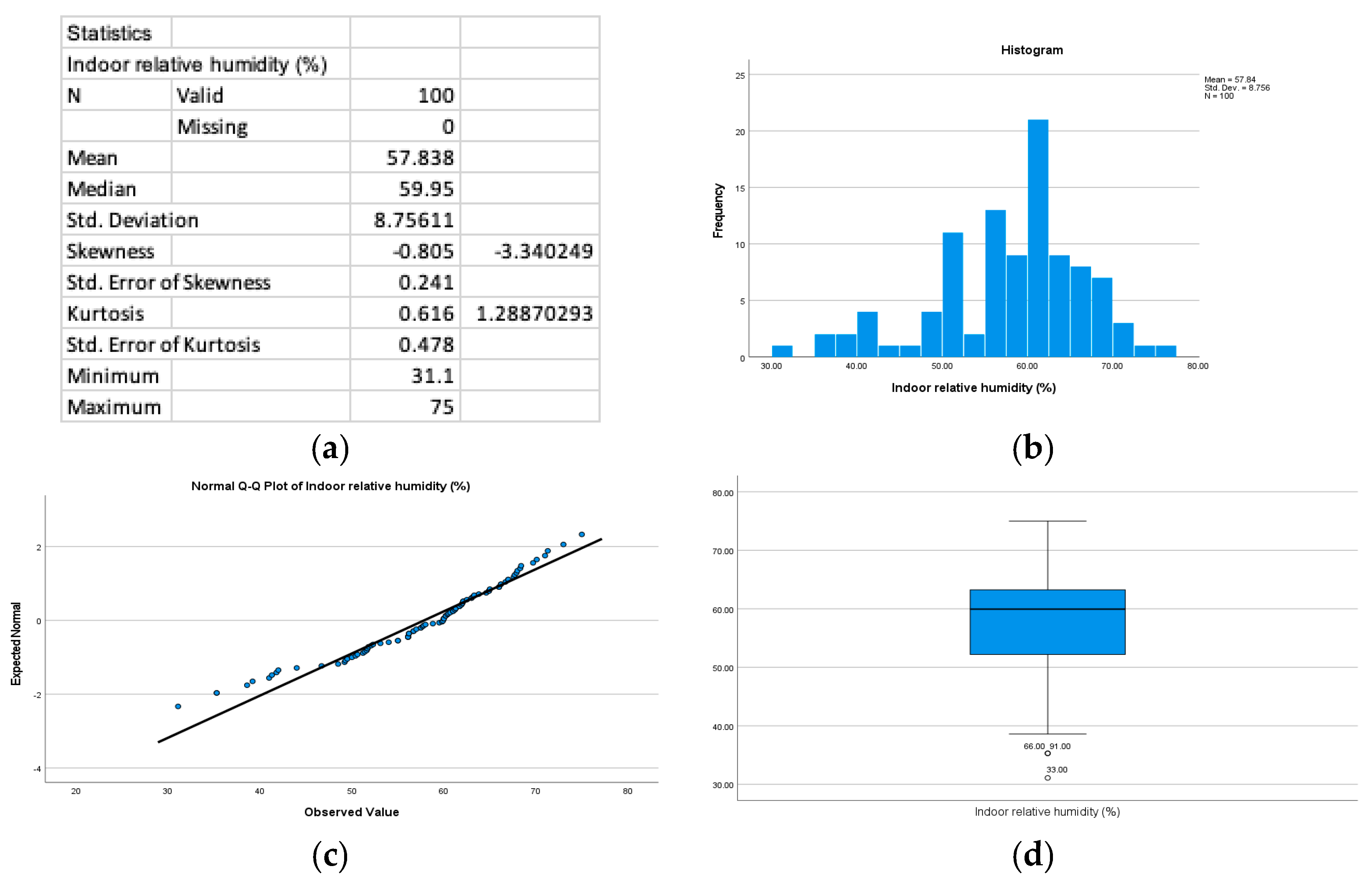

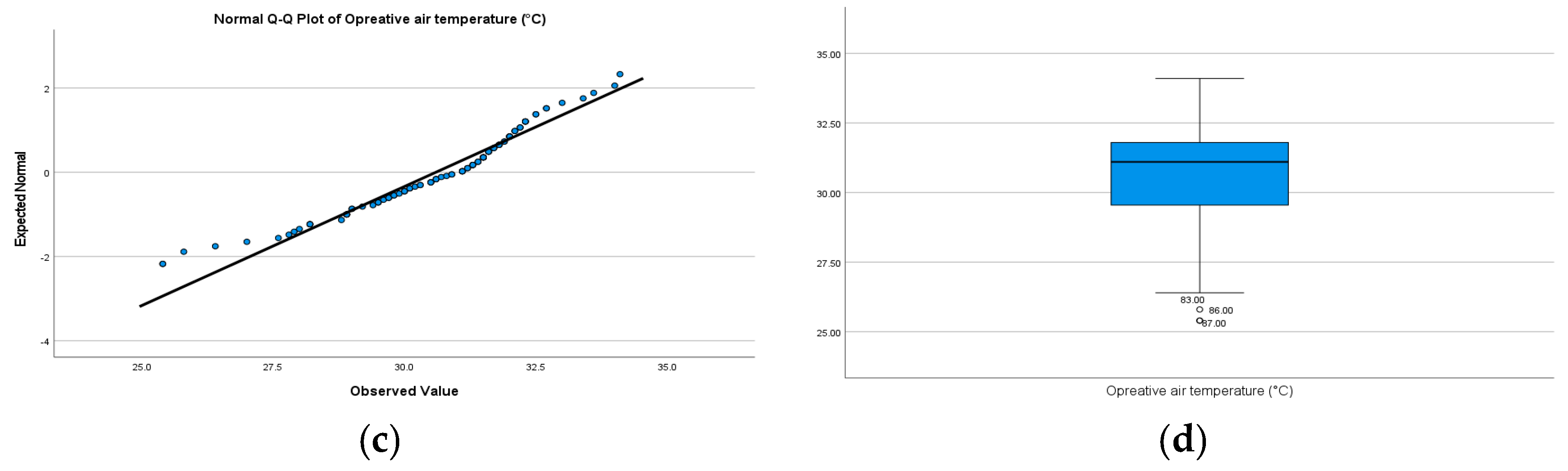
Disclaimer/Publisher’s Note: The statements, opinions and data contained in all publications are solely those of the individual author(s) and contributor(s) and not of MDPI and/or the editor(s). MDPI and/or the editor(s) disclaim responsibility for any injury to people or property resulting from any ideas, methods, instructions or products referred to in the content. |
© 2024 by the authors. Licensee MDPI, Basel, Switzerland. This article is an open access article distributed under the terms and conditions of the Creative Commons Attribution (CC BY) license (https://creativecommons.org/licenses/by/4.0/).