Abstract
In order to establish an optimal model for reasonably predicting the uniaxial compressive strength (UCS) of rocks, a method based on feature optimization and SSA-XGBoost was proposed. Firstly, the UCS predictor system of rocks, considering petrographic and physical parameters, was determined based on the systematic discussion of the factors affecting the UCS of rocks. Then, a feature selection method combining the RReliefF algorithm and Pearson correlation coefficient was proposed to further determine the optional input features. The XGBoost algorithm was used to establish the prediction model for rock UCS. In the process of model training, the Sparrow Search Algorithm (SSA) was used to optimize the hyperparameters. Finally, model evaluation was carried out to test the performance of the UCS prediction model. The method was applied and validated in a granitic tunnel. The results show that the proposed UCS prediction model can effectively predict the UCS of granitic rocks. Compared with simply adopting petrographic or physical parameters as the input features of the model, the UCS predictor considering petrographic and physical characteristics can improve the generalization ability of the SSA-XGBoost UCS prediction model effectively. The prediction method proposed in this study is reasonable and can provide some reference for establishing a universal method for accurately and quickly predicting the UCS of rocks.
1. Introduction
The uniaxial compressive strength is an important parameter reflecting the mechanical properties of rocks and is the basic basis for determining the design and construction programs of geotechnical engineering. Determining the UCS of rocks quickly and accurately is very important for geotechnical engineering. The conventional method for determining the UCS of rocks is to carry out uniaxial compression tests indoors. This method must comply with the appropriate standards, and the requirements for sampling, specimen processing, and transportation are stringent [1]. Therefore, although the accuracy of this testing method is very high, its economy and timeliness are poor. It is challenging to meet the needs of engineering sites.
In order to overcome these problems, many researchers have devoted themselves to seeking an indirect method for predicting the UCS of rocks that is economical and easy to implement in engineering sites. The first methods that have been proposed to indirectly predict the UCS of rocks include point load tests, density tests, Schmidt rebound tests, and ultrasonic tests. Based on one or several indices of the above methods, conventional simple regression or multiple regression analyses have been used to predict the UCS. These methods have the advantages of low cost, simple operation, and easy acquisition of results. However, due to the limitations of empirical formulae, the results reported in these studies have a limited range of application. With the development of artificial intelligence, machine learning is gradually being applied to the field of rock mechanics. Due to its advantages of being data-driven and not limited to a fixed form of equations, it has a wider range of applications. Dehghan et al. [2] predicted the UCS of rocks using an artificial neural network by considering parameters such as P-wave velocity, point load index, rebound value, and porosity. Rabbani et al. [3] used petrophysical parameters such as porosity, density, and saturation as predictors and combined them with an artificial neural network to predict the UCS of rocks. Mohamad et al. [4] used the volume density, tensile strength, point load index, and P-wave velocity as input parameters to predict the UCS of rocks using a hybrid neural network prediction model based on a particle swarm algorithm. Aboutaleb et al. [5] used rock density, primary wave velocity, and shear wave velocity as input variables and used an artificial neural network and support vector machine to establish a rock UCS prediction model. Fang et al. [6] constructed a UCS prediction model for granite using multiple neural networks by using the point load index, rebound value, p-wave velocity, and porosity as the predictors. They optimized the ANN weight and bias values using optimization algorithms for rock strength prediction and compared the results with those of the ANN itself. Unlike general engineering materials, rocks are mineral assemblages formed under long periods of diagenesis and geological evolution. In geology, rocks are identified and classified mainly by their petrographic characteristics, such as minerals and texture. Petrographic characteristics, as the inherent geological properties of rocks, determine not only the type of rock but also various physical and mechanical properties of rocks. Some researchers have also predicted the UCS of rocks from the petrographic perspective. Zorlu et al. [7] developed two UCS prediction models, multivariate regression and an artificial neural network, based on three petrographic parameters, namely, quartz content, stacking density, and concave–convex grain contact. Yesiloglu-Gultekin et al. [8,9] used the contents of quartz, orthoclase, and plagioclase as input parameters and the adaptive neuro-fuzzy inference system (ANFIS) to effectively estimate the UCS of granite in Türkiye. Khanlari et al. [10] established an optimal equation for predicting the UCS of rock based on packing proximity and packing density. Saedi and Mohammadi [11] selected indicators such as mineral content, mineral grain size, mineral shape, and fabric coefficient to predict the UCS of migmatites by constructing an artificial neural network (ANN) model.
All of the above findings indicated that machine learning algorithms are an effective way to achieve the prediction of rocks’ UCS. However, an excellent prediction model depends not only on the performance of the machine learning algorithm but also on the input features of the prediction model, i.e., the predictors. If the selection of predictors is not reasonable, it will easily lead to overfitting or underfitting of the prediction model. In previous research, the selection of predictors was mostly a simple combination of several parameters related to the UCS of rocks; the basis and rationality of the selected indices were not systematically demonstrated, so the proposed prediction model has limitations in both accuracy and applicability. In addition, the acquisition of some predictors is time-consuming and laborious, which leads to the poor engineering practicability of the proposed UCS prediction method.
In order to solve the above problems, a method for predicting the UCS of rocks based on feature optimization and SSA-XGBoost was proposed. The method mainly consists of UCS predictor system determination, feature selection, SSA-XGBoost model construction, and model evaluation. The rock UCS predictor system, considering petrographic and physical parameters, was determined based on the systematic discussion of the factors affecting the UCS of rocks, and a feature selection method combining the RReliefF algorithm and Pearson correlation coefficient was proposed to further determine the optional input features. The XGBoost algorithm was used to establish the prediction model for rock UCS. In the process of model training, the SSA was used to optimize the hyperparameters, and then the optimal SSA-XGBoost UCS prediction model was established. Finally, an engineering application was carried out relying on a granitic tunnel. The prediction method proposed in this study can provide the optional input features and, combined with the SSA-XGBoost algorithm, effectively improve the performance of rock UCS prediction.
2. Prediction Methodology for Uniaxial Compressive Strength of Rock
The method for predicting the uniaxial compressive strength of rocks based on feature optimization and SSA-XGBoost mainly consists of four parts:
- (1)
- UCS predictor system determination: The UCS predictor system of rocks was determined in terms of both petrographic characteristics and physical characteristics.
- (2)
- Feature selection: The RReliefF algorithm combined with the Pearson correlation coefficient was used to test the validity and select each input feature of the UCS predictor system, and then the input features used for training the prediction model were determined.
- (3)
- SSA-XGBoost model construction: Using the global optimization ability of the Sparrow Search Algorithm, the hyperparameters of XGBoost were continuously optimized iteratively in the set search space to acquire the optimal hyperparameter combinations, so as to establish the optimal SSA-XGBoost UCS prediction model.
- (4)
- Model evaluation: The coefficient of determination (R2), the root-mean-square error (RMSE), and the mean absolute percentage error (MAPE) were selected as evaluation indices to evaluate the performance of the SSA-XGBoost compressive strength prediction model.
2.1. UCS Predictor System Determination
The establishment of a scientific and reasonable UCS predictor system is an important prerequisite to ensure the prediction performance of the UCS prediction model. When determining the UCS predictor system for rocks, two basic principles should be followed: The first is that the relationship between the selected predictors and the UCS of rocks should be close, and the influence of the predictors on the UCS of rocks should be complementary (that is, it reflects different aspects that affect the UCS of rocks). The second is that the selected predictors should be easy to acquire, and the acquisition method should be as simple as possible and less time-consuming. In this study, based on a comprehensive analysis of the previous research results, the UCS predictor system for rocks was determined in terms of both petrographic characteristics and physical characteristics.
2.1.1. Petrographic Characteristics
As inherent geological characteristics of rocks, petrographic characteristics not only determine the rock type but also determine various physical and mechanical properties of rocks. Petrographic characteristics mainly include two aspects: mineral composition, and textural characteristics. Among them, minerals are the material basis of rocks; different minerals have different physical and mechanical properties, and the types of minerals and their contents are among the important factors determining the mechanical properties of rocks. Many scholars have studied the effect of the mineral composition of rocks on their UCS.
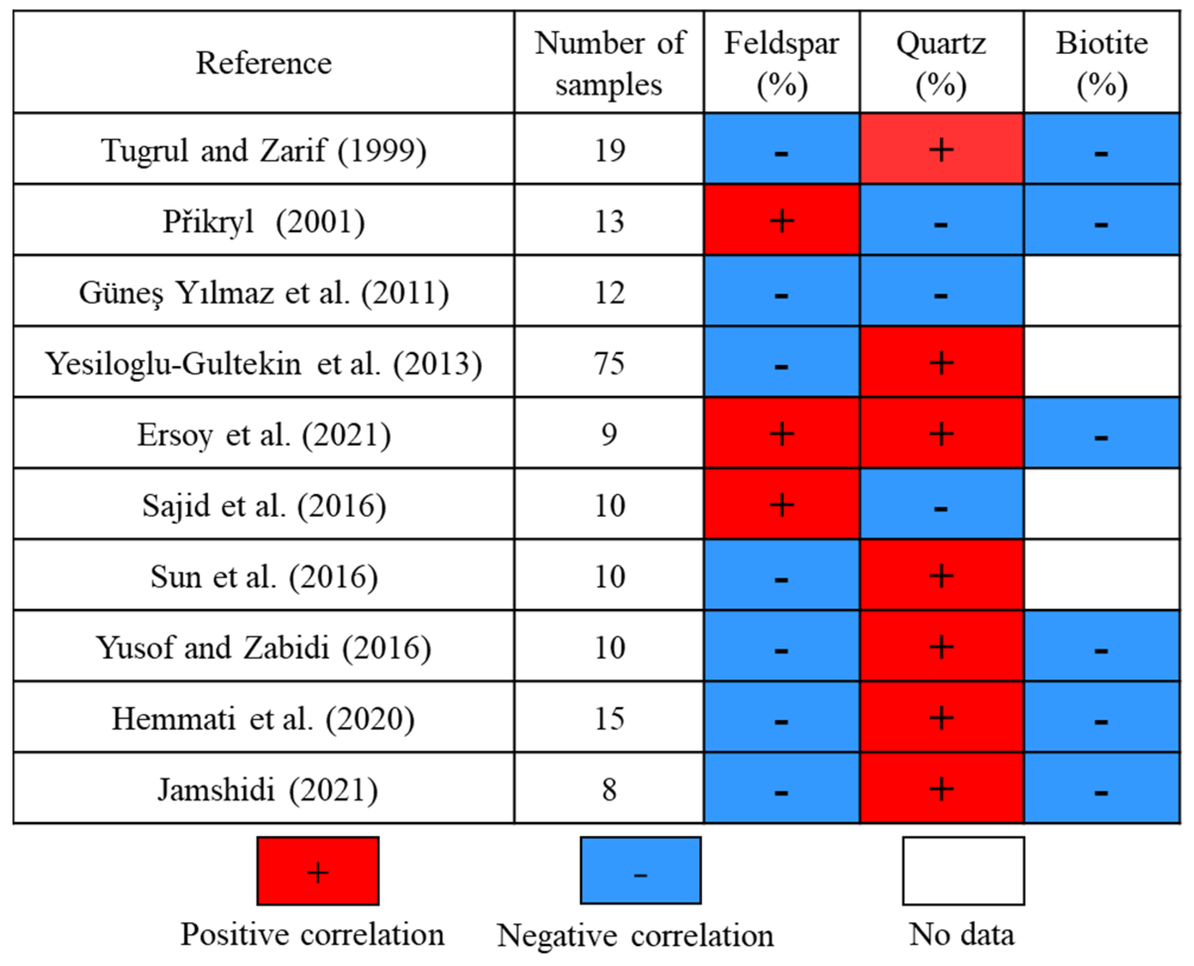
The following is an example of granitic rocks: The main minerals of granitic rocks include quartz, plagioclase, and K-feldspar, and they also contain certain amounts of dark minerals such as biotite or hornblende. Since K-feldspar and plagioclase are only slightly different in chemical composition, their crystal structures and physical properties are similar. Therefore, they can be unified as feldspar to study their mechanical properties [12]. Figure 1 shows the relationship between the mineral composition of granitic rocks and their UCS from previous studies. The red regions show a positive correlation, the blue regions show a negative correlation, and the white regions indicate the absence of data. As can be seen from Figure 1, the previous studies have shown that there is a significant correlation between feldspar, quartz content, and UCS. The disagreement lies in whether they are positively or negatively correlated with UCS. In addition, there are also disagreements about the relationship between biotite and UCS, with some studies suggesting a negative correlation and others suggesting no relationship. However, regardless of the relationship between minerals and UCS, it has been shown that the mineral composition of rocks has a significant effect on their UCS.
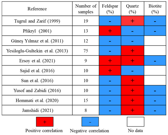
Figure 1.
Relationship between mineral composition and UCS of granitic rocks [8,13,14,15,16,17,18,19,20,21].
The textural characteristics of rocks mainly refer to the grain size, grain shape, and the interrelationship between grains in rock. Among them, the parameters characterizing the grain size include grain diameter, area, perimeter, etc. The parameters characterizing the grain shape include grain aspect ratio, roundness, preferred grain direction, shape factor, etc. The parameters characterizing the interrelationship between grains include the interlocking index and sorting coefficient. The textural characteristics of rocks affect the generation, expansion, and penetration of intergranular cracks in the rock damage process, which, in turn, control the UCS of rocks.
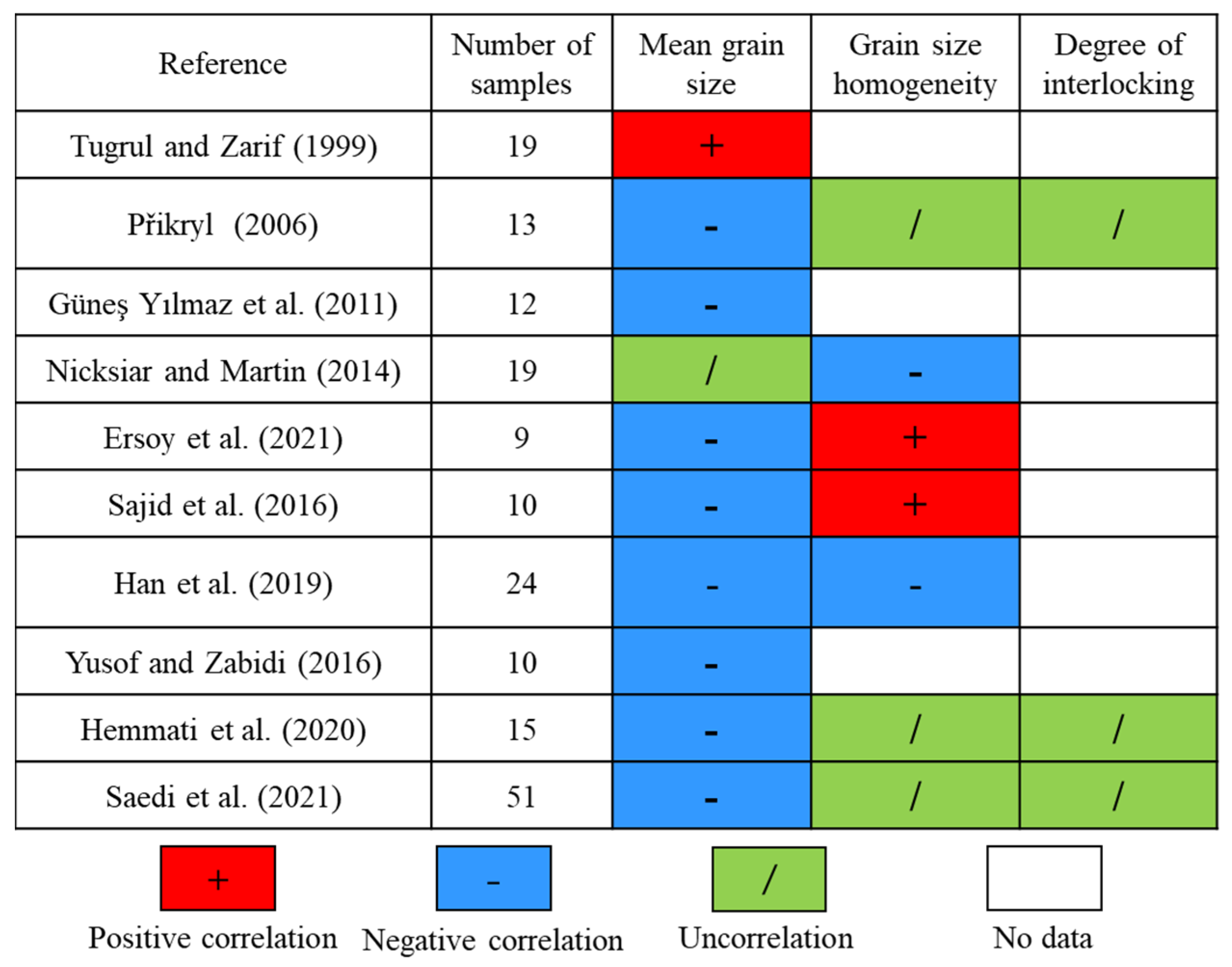
The following is an example of granitic rocks: The previous studies on the effects of textural parameters on UCS have focused on three aspects: mean grain size, grain size homogeneity, and degree of interlocking. The research generally concludes that both the size and the inhomogeneity of grains will have a certain effect on UCS, while the effect of the degree of interlocking on UCS is not significant (Figure 2). In addition, granitic rocks, as intrusive rocks formed by the cooling and crystallization of magma, have a holocrystalline texture, and their mineral grain size is generally up to the millimeter level. The mean grain size and distribution characteristics of mineral grains can be acquired from the macro-photographs of granitic rocks combined with digital image technology, while the other textural parameters need to be acquired from microphotographs of rock sheets, which is time-consuming and labor-intensive.

Figure 2.
Relationship between textural characteristics and UCS [11,13,15,16,17,19,20,22,23,24].
In summary, the mineral composition and textural characteristics of rocks were selected as the primary considerations for determining the UCS predictor system in this study.
2.1.2. Physical Characteristics
As a product of geological history, petrographic characteristics determine the physical and mechanical properties of rocks. From the studies of rock mechanics and geotechnical engineering, it is known that initial defects such as weathering, microcracks, and fissures due to exogenous and endogenous geological processes play an important role in the alteration of the mechanical properties of the rock, and they can even influence the alteration of the mechanical constitutive model. Therefore, some physical parameters that can reflect the initial defects inside the rock should be considered when constructing the rock UCS predictor system.
Ultrasonic testing technology is widely used in the field of geotechnical engineering due to its advantages of no sampling, non-destructive testing, convenience, and speed [25]. Based on the elastic wave propagation theory, the propagation velocity of ultrasonic waves in rock is a function of the density and elastic parameters of the medium. In general, the denser the rock, the faster the propagation speed of sound waves. When the ultrasonic wave propagating in the rock meets cracks or other fillings, it will be reflected, scattered, and diffracted, reducing the wave speed to a certain extent. It can be seen that the velocity of the ultrasonic waves can reflect the elastic properties, density, and internal defects of the rock, and these conditions have an important relationship with the UCS of the rock. A large number of scholars have researched the prediction of rocks’ UCS based on the P-wave velocity and established relevant prediction formulae (Table 1). Therefore, in this study, the P-wave velocity of the rock was selected as an input parameter in the UCS prediction model.

Table 1.
Relationship between P-wave velocity and UCS of rocks.
The Schmidt rebound test is another method used to evaluate rock strength, offering the advantages of portability, ease of operation, and non-destructive testing. Based on the Schmidt rebound test principle, the rebound value reflects the surface hardness of the rock, which is primarily determined by the mineral composition of the rock and the connection between the minerals [34]. When the minerals in the rock are weathered, the surface hardness will decrease and the rebound value will change. Therefore, the rebound value can reflect the mineral characteristics of the rock and its degree of weathering to a certain extent, and these factors are closely related to the UCS of the rock. A large number of scholars have investigated the correlation between rebound values and rock strength and established relevant mathematical expressions (Table 2). Therefore, in this study, the rebound value was selected as another input parameter in the UCS prediction model.
Table 2.
Relationship between rebound values and UCS of rocks.
In summary, the above two physical parameters, which can reflect the initial defects of the rock, were selected as important supplementary factors in determining the rock UCS predictor system in this study.
2.2. Feature Selection
Before using the machine learning algorithm to establish the rock UCS prediction model, the input feature data used for model training should be tested for validity to ensure the validity of each input feature and optimize the rock UCS predictor system, which, in turn, improves the performance of the rock UCS prediction model. A method combining the RReliefF algorithm with the Pearson correlation coefficient was proposed to test the validity of input features and select them.
The RReliefF algorithm is a classical filtered feature selection algorithm, improved from the Relief algorithm, specifically designed to solve the feature selection problem for regression models. Since the predicted values in the regression problem are continuous, the RReliefF algorithm establishes a model by introducing the probability of two dissimilar instances [42]:
where diff.value (A) is the difference of the instance on attribute A, diff.prediction is the predicted difference for the instance, PdiffA is the difference of probability for the nearest instances on attribute A, PdiffC is the difference of probability in prediction for the nearest instances, and PdiffC|diffA is the difference of probability between predictions for the nearest instances with differences on attribute A.
According to Bayes’ rule, the W(A) of the quality of attribute A is expressed as follows:
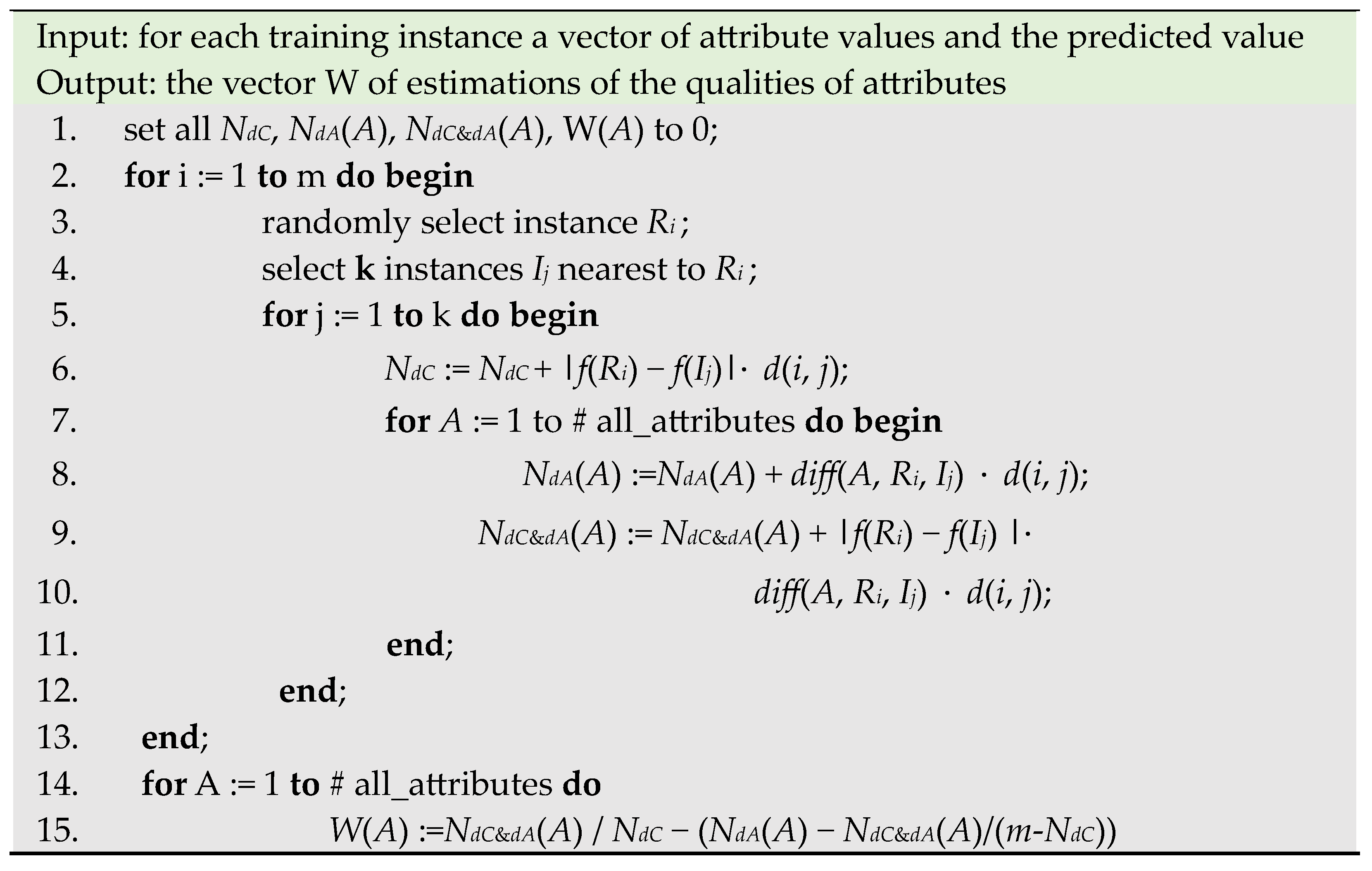
W(A) can be estimated by combining the above Equations (1)–(4). This can be achieved by the algorithm in Figure 3 [42], where NdC is the weight for different prediction, NdA(A) is the weight for different attribute, and NdC&dA(A) is the weight for different prediction and different attribute. The final estimation of each attribute W(A) is computed in lines 14 and 15.
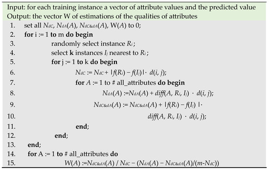
Figure 3.
Pseudocode of RReliefF.
For a machine learning model, if there is a large correlation between the input features, it will have an influence on the stability and accuracy of the model. In order to reduce the repetitive interference in the dataset caused by the large correlation between the input features, and to determine the optimal combination of input features, this study adopted the Pearson correlation coefficient for the secondary screening of the selected input features.
The Pearson correlation coefficient between the two variables can be calculated from Equation (5):
where r is the Pearson correlation coefficient in the range [−1,1], is the mean value of x, is the mean value of y, and n is the total number of samples.
When the absolute value of r is large, the correlation between the two variables is strong; when the absolute correlation coefficient of r is small, the correlation between variables is weak, and the range of r is −1 to 1. According to Smith [43], a value of |r| greater than 0.8 indicates a strong correlation between the parameters, and a value less than 0.2 indicates a weak correlation between the parameters.
In summary, the RReliefF algorithm can calculate the contribution of each feature index to the prediction of rocks’ UCS, and the Pearson correlation coefficient can determine the degree of correlation between each feature index. Combining the two, the features with larger feature weights and weaker correlation with other features can be retained, thus completing the selection of the optimal feature combination. The flow of the RReliefF–Pearson feature selection method proposed in this study is shown in Figure 4.
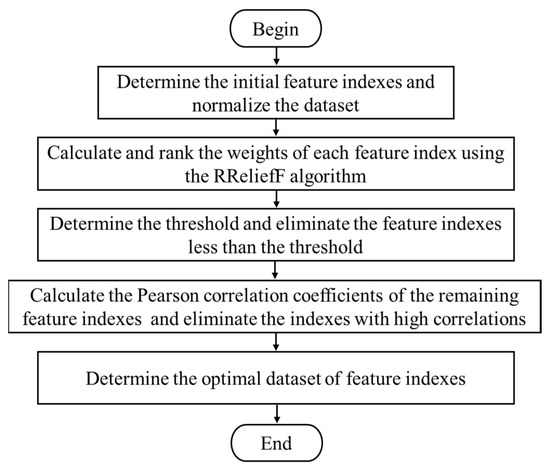
Figure 4.
Flowchart of the RReliefF–Pearson feature selection method.
2.3. SSA-XGBoost Model Construction
The XGBoost algorithm was adopted to mine the complex nonlinear relationship between the feature indices and rock UCS, and to predict the UCS of rocks. The Sparrow Search Algorithm was used to optimize the hyperparameters during the process of model training, and then the SSA-XGBoost rock UCS prediction model was finally established.
The SSA is a meta-heuristic optimization algorithm inspired by nature. Compared with the conventional optimization algorithms, such as grid search, random search, and Bayesian optimization, the SSA has a good ability to explore the potential region of the global optimum; hence, the local optimum issue is avoided effectively [44,45]. It can enable the automatic hyperparameter optimization of the XGBoost intensity prediction model to achieve the best prediction result. In the SSA, the entire sparrow population consists of producers, scroungers, and a small percentage of sparrows who perceive the danger. The SSA first sets parameters such as the number of sparrows in the initial population and the maximum number of iterations, calculates the fitness value of the initial population, and selects the current maximum and minimum values. The location information of the producers, scroungers, and sparrows who perceive the danger is then updated once. Finally, the current optimal solution is calculated. If the current optimal value is better than the optimal solution of the previous iteration, the location information update operation is performed. Otherwise, the position information is not updated, and the iterative operation is continued until the condition is satisfied. Finally, the global optimal value and the optimal fitness value are achieved. The detailed mathematical principles and establishment process of the SSA can be found in the publication of Xue and Shen [44].
XGBoost, as a typical ensemble learning algorithm based on the idea of boosting, is improved based on the Gradient-Boosting Decision Tree (GBDT). The core idea of this algorithm is to train the decision tree based on the residual between the predicted value and the measured value of the previous decision tree. Through multiple iterations of fitting the residual, it continuously approaches the measured value, reaches the set threshold or number of iterations, and ends the training. The predicted results of each decision tree are weighted and summed to acquire the final prediction result. Compared with GBDT, XGBoost performs second-order Taylor expansion on the loss function and adds a regularization term to the objective function to find the overall optimal solution, balancing the complexity of the objective function and the model. It has higher computational efficiency and anti-overfitting ability.
The XGBoost objective function is superimposed on the loss function, and the penalty function is denoted as follows:
The regularization item is
where Obj is the objective function; l is the loss function term, i.e., the training error; yi is the actual value; Ω(fk) is the regularization item to prevent overfitting; T and w denote the number of leaf nodes and the weights, respectively; γ is the leaf–tree penalization regularity term; and λ is the leaf-weight penalization regularity term.
The XGBoost ensemble learning model includes several hyperparameters, such as n_estimators, which represents the number of weak learners and affects the ensemble performance of the model. Parameters like max_depth, subsample, and max_leaves can be adjusted to control the model’s degree of fitting. To identify the optimal hyperparameters and achieve the optimal rock strength prediction model, this study employed the Sparrow Search Algorithm for optimization. Based on conclusions from previous research, four hyperparameters that significantly impact the model’s predictive performance were selected for optimization [46]. The specific parameters and their search ranges are shown in Table 3. Other non-optimized hyperparameters in XGBoost were set to their default values.
Table 3.
Introduction to XGBoost optimization hyperparameters and optimal searching range.
The process of establishing the SSA-XGBoost rock UCS prediction model is shown in Figure 5. The specific steps of the process were as follows:
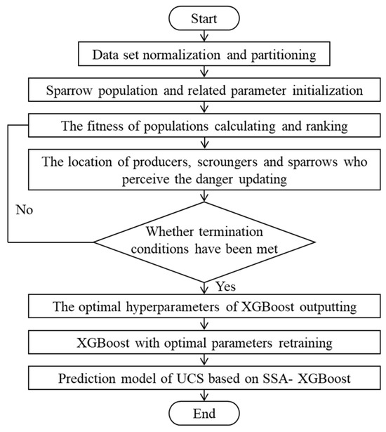
Figure 5.
The establishment process of the SSA-XGBoost rock UCS prediction model.
- (1)
- Standardize the data for each input feature, and then split the dataset with a training-to-test ratio of 8:2.
- (2)
- The sparrow population and the model-related parameters are initialized.
- (3)
- Using the Sparrow Search Algorithm (SSA), calculate the fitness value of each individual sparrow and record the best position.
- (4)
- Based on the rules of the Sparrow Search Algorithm, update the positions of producers, scroungers, and sparrows who perceive the danger to search for the optimal hyperparameters and model structure.
- (5)
- Determine whether the stopping conditions of the algorithm are met. If so, output the optimized hyperparameters; otherwise, return to Step 2 and continue the iterative optimization process.
- (6)
- Apply the acquired optimal combination of hyperparameters to the XGBoost algorithm and retrain the model to generate the SSA-XGBoost rock UCS prediction model.
2.4. Model Evaluation
The SSA-XGBoost model was retrained with the original training dataset and evaluated with the test dataset for prediction performance. The coefficient of determination (R2), the root-mean-square error (RMSE), and the mean absolute percentage error (MAPE) were used as the evaluation indices to compare the predicted and measured values of rock UCS. Among them, R2 indicates the accuracy of the model fitting data, and the closer it is to 1, the better the fitting effect is. RMSE indicates the degree of deviation between the model-predicted value and the measured value, while MAPE indicates the average of the absolute error between the model-predicted value and the measured value; the smaller the value of both, the better the model’s prediction performance.
3. Case Study and Application
The granitic rock of a tunnel project was taken as the research object. On the basis of acquiring the petrographic characteristics and physical characteristics, the rock UCS predictor system and the corresponding database were determined. The method combining the RReliefF algorithm with the Pearson correlation coefficient was used to select the important features, and the optimal input features were determined. Then, the data of the optimal input features were input into the SSA-XGBoost model for training and rock UCS prediction, and the prediction results were evaluated to verify the effectiveness of the rock UCS prediction method proposed in this study.
3.1. UCS Predictor System Determination
The granitic samples in this study were the same as in the study of Xie et al. [47]. The petrographic and mechanical parameters of the rocks were also derived from that paper (Table 4). In addition, this study also carried out a rebound test and acoustic test on 40 groups of granitic rocks from that paper, and the results are shown in Table 4.
Table 4.
Descriptive statistics of the database in this research.
3.2. Feature Selection
In this study, the number of nearest neighbors was taken as 10, and the calculation was repeated 30 times. The final weight values of the feature indices and the ranking by weight value from largest to smallest are shown in Figure 6. The larger the weight values of the feature indices, the more favorable the feature indices are for predicting the rock’s UCS, so the weight values should be as large as possible and the number of feature indices should not be too small. From Figure 6, it can be seen that the weights of the longitudinal P-wave velocity, sorting coefficient, rebound value, mean grain size, feldspar content, and quartz content were larger and more than 0.5, while the weight of the dark mineral content was only 0.003, which is much smaller than the weights of the other feature indices. Therefore, the dark mineral content was removed, and the other six feature indices were preliminarily selected, including feldspar content, quartz content, mean grain size, sorting coefficient, rebound value, and P-wave velocity.
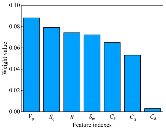
Figure 6.
The results of the calculation and ranking of weight values.
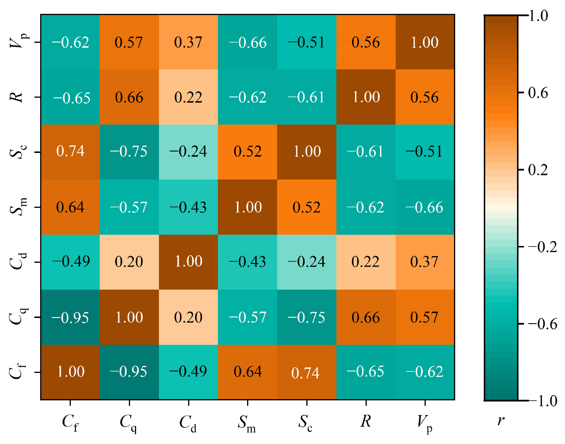
The Pearson correlation coefficient was used for secondary selection of the above six feature indices, and the results are shown in Figure 7. From Figure 7, it can be seen that the correlation coefficient between feldspar content and quartz content is 0.95, and there is strong correlation. Therefore, one of these two feature indices should be removed in order to reduce the multicollinearity between the feature indices.

Figure 7.
Heatmap among various feature indices.
According to the conclusions of Xie et al. [47], the content of feldspar was the main controlling factor affecting the UCS of the studied rocks. Therefore, the quartz content was removed, and the other five feature indices were ultimately selected, including feldspar content, mean grain size, sorting coefficient, rebound value, and P-wave velocity.
3.3. SSA-XGBoost Model Construction
When training the model, the dataset was divided into a training set (32 groups) and a test set (8 groups) at a ratio of 8:2, which were used for training and validation of the model, respectively. During the model training process, after several iterations, the SSA’s four hyperparameter optimization results for XGBoost were n_estimators = 83, max_depth = 17, eta = 0.90, and subsample = 0.85.
3.4. Model Evaluation
Figure 8 shows the training and prediction results of the SSA-XGBoost rock UCS prediction model. As can be seen from the figure, the scatter distribution of the model in the training set is near the reference line with slope 1, R2 is 0.999, the RMSE is 0.17, and the MAPE is 0.18%. This indicates that the model has superior learning ability for complex nonlinear relationships in known data.
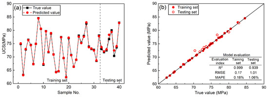
Figure 8.
The results of the SSA-XGBoost rock UCS prediction model considering petrographic and physical parameters: (a) Comparison of predicted values and true values, the dashed line is the division of training set and test set. (b) Results of model evaluation, the oblique line is a contour line indicating that the true values and the predicted values are equal.
The key to evaluating the strength of a prediction model is its ability to generalize to unknown data, i.e., its performance on the testing set. As can be seen in Figure 8, the model had an R2 of 0.939, RMSE of 1.01, and MAPE of 1.06% on the testing set. Although the performance was slightly worse than on the training set, it still showed good generalization ability. Therefore, the SSA-XGBoost strength prediction model proposed in this study, which combines rocks’ petrographic and physical parameters, can achieve the fast and effective prediction of rock UCS.
4. Discussion
4.1. Comparison of the Performance of XGBoost and SSA-XGBoost
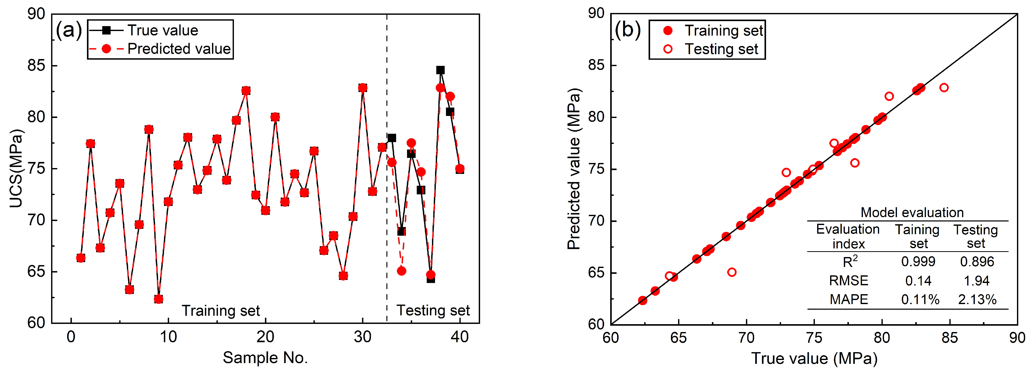
In order to verify the superiority of the SSA, an XGBoost rock UCS prediction model considering petrographic and physical parameters was established. The default hyperparameters of XGBoost were used during the model training. The training and prediction results of the XGBoost UCS prediction model considering petrographic and physical parameters can be seen in Figure 9. It can be seen that the predicted values and true values of this prediction model were almost the same on the training set, but there was a significant deviation between the predicted values and the true values for the test set. According to the evaluation indices in Figure 9b, R2 is also above 0.99, the RMSE is 0.14, and the MAPE is 0.11%, still showing excellent learning ability of the model. However, in the test set, R2 is 0.896, the RMSE is 1.94, and the MAPE is 2.13%.

Figure 9.
The results of the XGBoost rock UCS prediction model considering petrographic and physical parameters: (a) Comparison of predicted values and true values, the dashed line is the division of training set and test set. (b) Results of model evaluation, the oblique line is a contour line indicating that the true values and the predicted values are equal.
This suggests that the performance of the XGBoost prediction model on the test set is significantly lower than that on the training set, and there is a certain degree of overfitting.
In addition, by comparing the evaluation indices of the XGBoost prediction model and SSA-XGBoost prediction model, it can be found that although the two models have excellent performance on the training set, the performance of the XGBoost prediction model on the test set is significantly lower than that of the SSA-XGBoost prediction model. The results show that, after optimizing the XGBoost hyperparameters with the SSA, the overfitting of the prediction model can be reduced to a certain extent, and its generalization ability can be improved.
4.2. Comparison of the Performance of Different Feature Indices
In order to verify the superiority of the proposed predictor system considering petrographic and physical parameters, this study used petrographic characteristics and physical parameters as input features of the prediction model, and the SSA-XGBoost algorithm was used for data training to establish the rock UCS prediction model. Among the input features based on petrographic parameters were the quartz content, feldspar content, dark mineral content, mean grain size, and sorting coefficient. The input features based on physical parameters included the rebound value and P-wave velocity. The optimized SSA-XGBoost model hyperparameter settings acquired after the model training are shown in Table 5.
Table 5.
Optimal hyperparameter settings in SSA-XGBoost models with different input features.
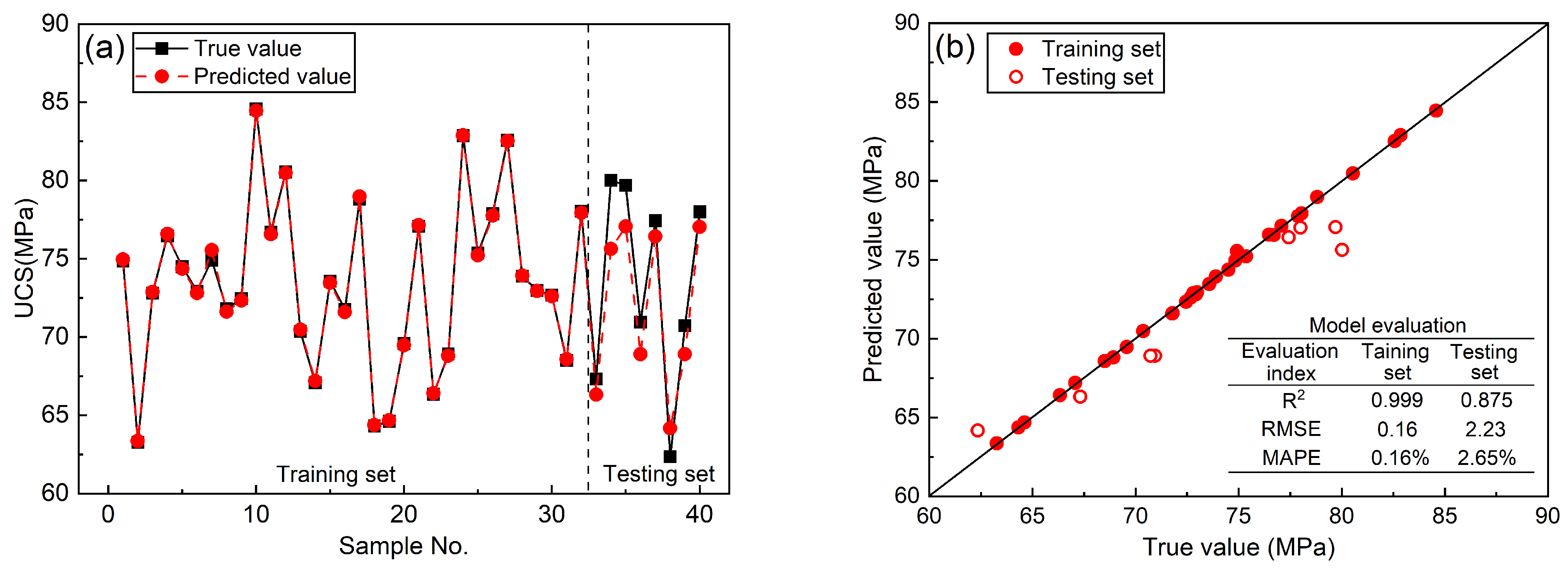
Figure 10 shows the training and prediction results of the SSA-XGBoost UCS prediction model based on petrographic parameters. From Figure 10a, it can be seen that the predicted values and true values of this prediction model were almost the same on the training set, but there was a significant deviation between the predicted values and true values on the testing set. According to the evaluation indices in Figure 10b, R2 is also above 0.99, the RMSE is 0.16, and the MAPE is 0.16%, still showing excellent learning ability of the model. However, on the test set, R2 is 0.875, the RMSE is 2.23, and the MAPE is 2.65%. This shows that the generalization ability of the model is significantly inferior to that of the SSA-XGBoost UCS prediction model that combines rocks’ petrographic and physical parameters. In addition, the performance of the model on the testing set was significantly lower than that on the training set, indicating that the overfitting of the model is serious.
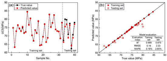
Figure 10.
The results of the SSA-XGBoost rock UCS prediction model based on petrographic parameters: (a) Comparison of predicted values and true values, the dashed line is the division of training set and test set. (b) Results of model evaluation, the oblique line is a contour line indicating that the true values and the predicted values are equal.
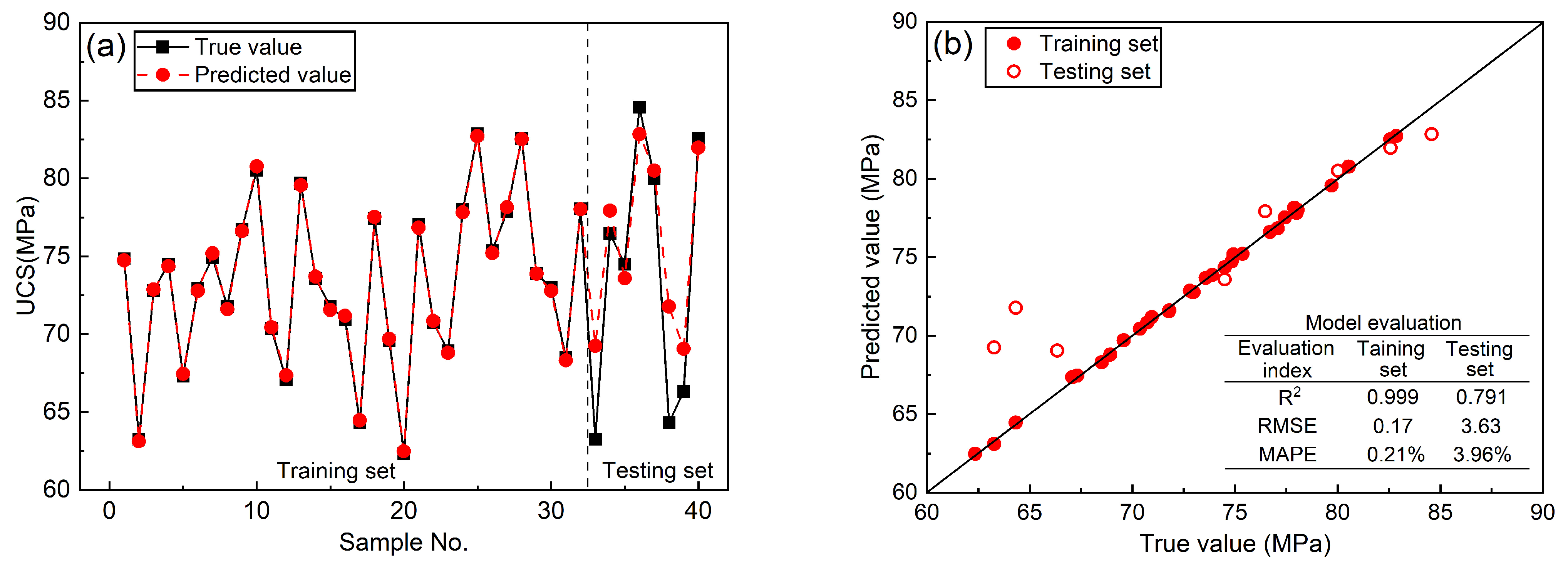
Figure 11 shows the training and prediction results of the SSA-XGBoost UCS prediction model based on physical parameters. As can also be seen in Figure 11a, the predicted values and true values of this prediction model were also closer on the training set, and there was still a significant deviation between the predicted values and true values on the testing set. According to the evaluation indices in Figure 11b, R2 is also above 0.99, the RMSE is 0.17, and the MAPE is 0.21%, which is essentially the same performance as the previous two models on the training set. On the testing set, R2 is 0.791, the RMSE is 3.63, and the MAPE is 3.96%. Compared with the first two models, the model trained with only two predictors (rebound value and P-wave velocity) had the worst generalization ability. Compared with the previous two prediction models, the gap between the performance of this model on the testing set and its performance on the training set is larger, indicating that the overfitting of the model is more serious.
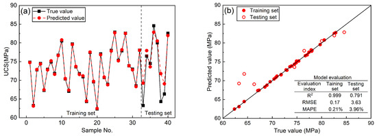
Figure 11.
The results of the SSA-XGBoost rock UCS prediction model based on physical parameters: (a) Comparison of predicted values and true values, the dashed line is the division of training set and test set. (b) Results of model evaluation, the oblique line is a contour line indicating that the true values and the predicted values are equal.
Ensemble models of trees are the most powerful learners among machine learning models, and while their accuracy is high, the risk of overfitting is equally high. The UCS predictor system considering petrographic and physical parameters and the SSA-XGBoost algorithm proposed in this study can effectively reduce the overfitting of the rock UCS prediction model and improve its generalization ability, so as to achieve effective prediction of rocks’ UCS. However, due to the small amount of data used in this study, there was still a certain degree of overfitting. Further expansion of the dataset should be a good solution to this problem.
4.3. Prospects for Rock UCS Prediction
The construction of prediction models using machine learning algorithms is an important way to achieve the fast prediction of rocks’ UCS. The accuracy and reliability of this approach depend on two main aspects: the quality and quantity of data on the one hand, and the performance of the machine learning algorithm on the other. In terms of data quality and data quantity, the index system constructed in this study for predicting the UCS of rocks, considering petrographic and physical parameters, ensures the quality of the model’s input parameters. In terms of machine learning algorithms, this study adopted XGBoost, which is a representative ensemble learning algorithm with stronger generalization ability than individual machine learning algorithms. The SSA was used to optimize the hyperparameters, and the prediction performance of the model was further improved. The research conducted in this study can provide some reference for establishing a fast prediction method for rock UCS with universal applicability, but the dataset used for prediction model training, and validation only included granitic rocks, so there are some limitations.
Granitic rocks are crystalline rocks formed by magma cooling and crystallizing in the deep crust, which have significant differences from rocks of other origins in terms of petrographic, physical, and mechanical properties. Therefore, the prediction model constructed in this study only proved a good prediction effect for granitic rocks, and its applicability to other types of rocks needs to be further discussed and verified. In addition, for the UCS prediction model constructed using machine learning algorithms, in order to ensure its strong generalization ability and applicability, it is necessary not only to ensure that the predictor system is established scientifically and reasonably but also to have a sufficient database.
In future studies, we propose carrying out the quantitative analysis of petrographic parameters and strength prediction of another type of rocks: terrigenous clastic rocks. While verifying the validity of the UCS predictor system constructed in this study, the training dataset will be further expanded. Eventually, a UCS prediction model with a wide range of applicability and strong generalization ability will be developed, and the model will be validated and evaluated in engineering.
5. Conclusions
In order to establish an optimal model for reasonably predicting the UCS of rocks, a method based on feature optimization and SSA-XGBoost is proposed in this study. Relying on a granitic tunnel, the reliability of the UCS prediction method was verified. The superiority and applicability of this model were discussed, and the specific conclusions can be summarized as follows:
- (1)
- The method for predicting the UCS of rocks based on feature optimization and SSA-XGBoost mainly consists of four parts: UCS predictor system determination, feature selection, SSA-XGBoost model construction, and model evaluation. The rock UCS predictor system, considering petrographic and physical parameters, was determined based on the systematic discussion of the factors affecting the UCS of rocks, and a feature selection method combining the RReliefF algorithm and Pearson correlation coefficient was proposed.
- (2)
- This method was applied and validated in a granitic tunnel. The results show that the coefficient of determination of the UCS prediction model based on SSA-XGBoost is 0.939, the root-mean-square error is 1.01, and the mean absolute percentage error is 1.06%. The established UCS prediction model based on SSA-XGBoost can effectively predict the UCS of granitic rocks.
- (3)
- Compared with simply adopting petrographic or physical parameters as the input features of the model, the UCS predictor system considering petrographic and physical characteristics can effectively improve the generalization ability of the prediction model. The predictor system proposed in this study is reasonable and can provide some reference for establishing a universal method for accurately and quickly predicting the UCS of rocks.
- (4)
- Since the SSA-XGBoost rock UCS prediction model relied only on the granitic rock dataset for training and validation, its generalizability needs to be further verified. However, based on specific projects and datasets of rocks, engineers can effectively utilize this method to establish a rock UCS prediction model that is suitable for their project.
Author Contributions
H.X. conducted the literature review and drafted the initial manuscript. P.L. developed the overarching research goals and edited the draft of manuscript. J.K. analyzed and interpreted the results of the study. C.Z. collected the test data for this research. Y.D. contributed substantially to data analysis, manuscript revisions, and provided critical insights that shaped the final version of the paper. All authors have read and agreed to the published version of the manuscript.
Funding
This research was funded by the National Natural Science Foundation of China (Grant No.: 52022053; 52009073) and the Natural Science Foundation of Shandong Province (Grant No.: ZR2023YQ049).
Institutional Review Board Statement
Not applicable.
Informed Consent Statement
Not applicable.
Data Availability Statement
The original contributions presented in the study are included in the article, further inquiries can be directed to the corresponding authors.
Conflicts of Interest
The authors declare no conflicts of interest.
References
- Bieniawski, Z.T. Estimating the strength of rock materials. J. South Afr. Inst. Min. Metall. 1974, 74, 312–320. [Google Scholar] [CrossRef]
- Dehghan, S.; Sattari, G.; Chehreh Chelgani, S.; Aliabadi, M.A. Prediction of uniaxial compressive strength and modulus of elasticity for Travertine samples using regression and artificial neural networks. Min. Sci. Technol. 2010, 20, 41–46. [Google Scholar] [CrossRef]
- Rabbani, E.; Sharif, F.; Koolivand Salooki, M.; Moradzadeh, A. Application of neural network technique for prediction of uniaxial compressive strength using reservoir formation properties. Int. J. Rock Mech. Min. 2012, 56, 100–111. [Google Scholar] [CrossRef]
- Mohamad, E.T.; Armaghani, D.J.; Momeni, E.; Abad, S.V.A.N. Prediction of the unconfined compressive strength of soft rocks; a PSO-based ANN approach. Bull. Eng. Geol. Environ. 2015, 74, 745–757. [Google Scholar] [CrossRef]
- Aboutaleb, S.; Bagherpour, R.; Behnia, M.; Aghababaei, M. Combination of the physical and ultrasonic tests in estimating the uniaxial compressive strength and Young’s modulus of intact limestone rocks. Geotech. Geol. Eng. 2017, 35, 3015–3023. [Google Scholar] [CrossRef]
- Fang, Q.; Yazdani Bejarbaneh, B.; Vatandoust, M.; Jahed Armaghani, D.; Ramesh Murlidhar, B.; Tonnizam Mohamad, E. Strength evaluation of granite block samples with different predictive models. Eng. Comput. 2021, 37, 891–908. [Google Scholar] [CrossRef]
- Zorlu, K.; Gokceoglu, C.; Ocakoglu, F.; Nefeslioglu, H.A.; Acikalin, S. Prediction of uniaxial compressive strength of sandstones using petrography-based models. Eng. Geol. 2008, 96, 141–158. [Google Scholar] [CrossRef]
- Yesiloglu-Gultekin, N.; Gokceoglu, C.; Sezer, E.A. Prediction of uniaxial compressive strength of granitic rocks by various nonlinear tools and comparison of their performances. Int. J. Rock Mech. Min. 2013, 62, 113–122. [Google Scholar] [CrossRef]
- Yesiloglu-Gultekin, N.; Sezer, E.A.; Gokceoglu, C.; Bayhan, H. An application of adaptive neuro fuzzy inference system for estimating the uniaxial compressive strength of certain granitic rocks from their mineral contents. Expert Syst. Appl. 2013, 40, 921–928. [Google Scholar] [CrossRef]
- Khanlari, G.R.; Heidari, M.; Noori, M.; Momeni, A. The Effect of Petrographic Characteristics on Engineering Properties of Conglomerates from Famenin Region, Northeast of Hamedan, Iran. Rock Mech. Rock Eng. 2016, 49, 2609–2621. [Google Scholar] [CrossRef]
- Saedi, B.; Mohammadi, S.D. Prediction of Uniaxial Compressive Strength and Elastic Modulus of Migmatites by Microstructural Characteristics Using Artificial Neural Networks. Rock Mech. Rock Eng. 2021, 54, 5617–5637. [Google Scholar] [CrossRef]
- He, C.; Mishra, B.; Shi, Q.; Zhao, Y.; Lin, D.; Wang, X. Correlations between mineral composition and mechanical properties of granite using digital image processing and discrete element method. Int. J. Min. Sci. Technol. 2023, 33, 949–962. [Google Scholar] [CrossRef]
- Tugrul, A.; Zarif, I.H. Correlation of mineralogical and textural characteristics with engineering properties of selected granitic rocks from Turkey. Eng. Geol. 1999, 51, 303–317. [Google Scholar] [CrossRef]
- Prikryl, R. Some microstructural aspects of strength variation in rocks. Int. J. Rock Mech. Min. Sci. 2001, 38, 671–682. [Google Scholar] [CrossRef]
- Güneş Yılmaz, N.; Mete Goktan, R.; Kibici, Y. Relations between some quantitative petrographic characteristics and mechanical strength properties of granitic building stones. Int. J. Rock Mech. Min. 2011, 48, 506–513. [Google Scholar] [CrossRef]
- Ersoy, H.; Karahan, M.; Kolaylı, H.; Sünnetci, M.O. Influence of Mineralogical and Micro-Structural Changes on the Physical and Strength Properties of Post-thermal-Treatment Clayey Rocks. Rock Mech. Rock Eng. 2021, 54, 679–694. [Google Scholar] [CrossRef]
- Sajid, M.; Coggan, J.; Arif, M.; Andersen, J.; Rollinson, G. Petrographic features as an effective indicator for the variation in strength of granites. Eng. Geol. 2016, 202, 44–54. [Google Scholar] [CrossRef]
- Sun, Q.; Zhang, J.; Wang, Z.; Zhang, H.; Fang, J. Segment wear characteristics of diamond frame saw when cutting different granite types. Diam. Relat. Mater. 2016, 68, 143–151. [Google Scholar] [CrossRef]
- Yusof, N.Q.A.M.; Zabidi, H. Correlation of Mineralogical and Textural Characteristics with Engineering Properties of Granitic Rock from Hulu Langat, Selangor. Procedia Chem. 2016, 19, 975–980. [Google Scholar] [CrossRef]
- Hemmati, A.; Ghafoori, M.; Moomivand, H.; Lashkaripour, G.R. The effect of mineralogy and textural characteristics on the strength of crystalline igneous rocks using image-based textural quantification. Eng. Geol. 2020, 266, 105467. [Google Scholar] [CrossRef]
- Jamshidi, A. Predicting the Strength of Granitic Stones after Freeze–Thaw Cycles: Considering the Petrographic Characteristics and a New Approach Using Petro-Mechanical Parameter. Rock Mech. Rock Eng. 2021, 54, 2829–2841. [Google Scholar] [CrossRef]
- Přikryl, R. Assessment of rock geomechanical quality by quantitative rock fabric coefficients: Limitations and possible source of misinterpretations. Eng. Geol. 2006, 87, 149–162. [Google Scholar] [CrossRef]
- Nicksiar, M.; Martin, C.D. Factors affecting crack initiation in low porosity crystalline rocks. Rock Mech. Rock Eng. 2014, 47, 1165–1181. [Google Scholar] [CrossRef]
- Han, Z.; Zhang, L.; Zhou, J.; Yuan, G.; Wang, P. Uniaxial compression test and numerical studies of grain size effect on mechanical properties of granite. J. Eng. Geol. 2019, 27, 497–504. [Google Scholar]
- Wang, Y.; Wang, R.; Wang, J.; Li, N.; Cao, H. A Rock Mass Strength Prediction Method Integrating Wave Velocity and Operational Parameters Based on the Bayesian Optimization Catboost Algorithm. KSCE J. Civ. Eng. 2023, 27, 3148–3162. [Google Scholar] [CrossRef]
- Meng, Z.P.; Zhang, J.C.; Tiedemann, J. Relationship between physical and mechanical parameters and acoustic wave velocity of coal measures rocks. Chin. J. Geophys. 2006, 49, 1505–1510. [Google Scholar]
- Deng, H.; Li, J.; Deng, C.; Wang, L.; Lu, T. Analysis of sampling in rock mechanics test and compressive strength prediction methods. Rock Soil. Mech. 2011, 32, 3399–3403. [Google Scholar]
- Moradian, Z.A.; Behnia, M. Predicting the Uniaxial Compressive Strength and Static Young’s Modulus of Intact Sedimentary Rocks Using the Ultrasonic Test. Int. J. Geomech. 2009, 9, 14–19. [Google Scholar] [CrossRef]
- Sharma, P.K.; Singh, T.N. A correlation between P-wave velocity, impact strength index, slake durability index and uniaxial compressive strength. Bull. Eng. Geol. Environ. 2008, 67, 17–22. [Google Scholar] [CrossRef]
- Kahraman, S. Evaluation of simple methods for assessing the uniaxial compressive strength of rock. Int. J. Rock Mech. Min. Sci. 2001, 38, 981–994. [Google Scholar] [CrossRef]
- Yasar, E.; Erdogan, Y. Correlating sound velocity with the density, compressive strength and Young’s modulus of carbonate rocks. Int. J. Rock Mech. Min. 2004, 41, 871–875. [Google Scholar] [CrossRef]
- Uyanık, O.; Sabbağ, N.; Uyanık, N.A.; Öncü, Z. Prediction of mechanical and physical properties of some sedimentary rocks from ultrasonic velocities. Bull. Eng. Geol. Environ. 2019, 78, 6003–6016. [Google Scholar] [CrossRef]
- Nefeslioglu, H.A. Evaluation of geo-mechanical properties of very weak and weak rock materials by using non-destructive techniques: Ultrasonic pulse velocity measurements and reflectance spectroscopy. Eng. Geol. 2013, 160, 8–20. [Google Scholar] [CrossRef]
- Rahimi, M.R.; Mohammadi, S.D.; Beydokhti, A.T. Correlation between Schmidt Hammer Hardness, Strength Properties and Mineral Compositions of Sulfate Rocks. Geotech. Geol. Eng. 2022, 40, 545–574. [Google Scholar] [CrossRef]
- Yilmaz, I.; Sendir, H. Correlation of Schmidt hardness with unconfined compressive strength and Young’s modulus in gypsum from Sivas (Turkey). Eng. Geol. 2002, 66, 211–219. [Google Scholar] [CrossRef]
- Aydin, A.; Basu, A. The Schmidt hammer in rock material characterization. Eng. Geol. 2005, 81, 1–14. [Google Scholar] [CrossRef]
- Fener, M.; Kahraman, S.; Bilgil, A.; Gunaydin, O. A Comparative Evaluation of Indirect Methods to Estimate the Compressive Strength of Rocks. Rock Mech. Rock Eng. 2005, 38, 329–343. [Google Scholar] [CrossRef]
- Gupta, V. Non-destructive testing of some Higher Himalayan rocks in the Satluj Valley. Bull. Eng. Geol. Environ. 2009, 68, 409–416. [Google Scholar] [CrossRef]
- Yagiz, S. Predicting uniaxial compressive strength, modulus of elasticity and index properties of rocks using the Schmidt hammer. Bull. Eng. Geol. Environ. 2009, 68, 55–63. [Google Scholar] [CrossRef]
- Bruno, G.; Vessia, G.; Bobbo, L. Statistical method for assessing the uniaxial compressive strength of carbonate rock by Schmidt hammer tests performed on core samples. Rock Mech. Rock Eng. 2013, 46, 199–206. [Google Scholar] [CrossRef]
- Wang, M.; Wan, W. A new empirical formula for evaluating uniaxial compressive strength using the Schmidt hammer test. Int. J. Rock Mech. Min. 2019, 123, 104094. [Google Scholar] [CrossRef]
- Robnik-Šikonja, M.; Kononenko, I. An adaptation of Relief for attribute estimation in regression. In Proceedings of the 14th International Conference on Machine Learning (ICML’ 97), Nashville, TN, USA, 8–12 July 1997; Volume 5, pp. 296–304. [Google Scholar]
- Smith, G.N. Probability and Statistics in Civil Engineering; Collins Professional and Technical Books; Collins: Cork, Ireland, 1986; 244p. [Google Scholar]
- Xue, J.; Shen, B. A novel swarm intelligence optimization approach: Sparrow search algorithm. Syst. Sci. Control Eng. 2020, 8, 22–34. [Google Scholar] [CrossRef]
- Xu, B.; Tan, Y.; Sun, W.; Ma, T.; Liu, H.; Wang, D. Study on the Prediction of the Uniaxial Compressive Strength of Rock Based on the SSA-XGBoost Model. Sustainability 2023, 15, 5201. [Google Scholar] [CrossRef]
- Bian, J.; Huo, R.; Zhong, Y.; Guo, Z. XGB-Northern Goshawk Optimization: Predicting the Compressive Strength of Self-Compacting Concrete. KSCE J. Civ. Eng. 2024, 28, 1423–1439. [Google Scholar] [CrossRef]
- Xie, H.; Yu, T.; Lin, P.; Wang, Z.; Xu, Z. Effect of petrographic characteristics on uniaxial compressive strength of granitic rocks from Xinjiang, China. J. Cent. South Univ. 2023, 30, 2340–2359. [Google Scholar] [CrossRef]


Disclaimer/Publisher’s Note: The statements, opinions and data contained in all publications are solely those of the individual author(s) and contributor(s) and not of MDPI and/or the editor(s). MDPI and/or the editor(s) disclaim responsibility for any injury to people or property resulting from any ideas, methods, instructions or products referred to in the content. |
© 2024 by the authors. Licensee MDPI, Basel, Switzerland. This article is an open access article distributed under the terms and conditions of the Creative Commons Attribution (CC BY) license (https://creativecommons.org/licenses/by/4.0/).