Optimizing the Operation of Grid-Interactive Efficient Buildings (GEBs) Using Machine Learning

Abstract

The building sector constitutes 40% of global electric energy consumption, making it vital to address for achieving the global net-zero emissions goal by 2050. This study focuses on enhancing electric load forecasting systems’ performance and interactivity by investigating the impact of weather and building usage parameters. Hourly electricity meter readings from a Texas university campus building (2012–2015) were employed, applying pre-processing techniques and machine learning algorithms such as linear regression, decision trees, and support vector machines using MATLAB R2023a. Exponential Gaussian Process Regression (GPR) showed the best performance at a one-year training data size, yielding an average normalized root mean square error (nRMSE) value of 0.52%, equivalent to a 0.3% reduction compared to leading methods. The developed system is presented through an interactive GUI and allows for prediction of external factors like PV and EV integration. Through a case study implementation, the combined system achieves 12.8% energy savings over a typical year simulated using ETAP 22 and Trimble ProDesign software version 2021.0.19. This holistic solution precisely models the electric demand management scenario of grid-interactive efficient buildings (GEBs), simultaneously enhancing reliability and flexibility to accommodate diverse applications.

1. Introduction

Buildings are essential for daily life in residential, commercial, and industrial settings. These contribute significantly to global energy consumption—about 40% of total electric energy usage [1]. Ongoing studies focus on optimizing building systems for substantial energy savings. Technological advancements make buildings “smarter”, enhancing not only their operations but also connectivity. This connectivity enables efficient information-sharing within centralized systems, improving data access for monitoring and control. Additionally, it facilitates advanced data management and analysis, leading to optimization in various aspects [1,2].

This section details all related technologies and methodologies to the development of a machine learning-based building to grid energy management system. Performances of existing systems were assessed, leading to the identification of research gaps that are addressed in this study.

The adoption of Building Management Systems (BMSs) is now prevalent in both new construction projects and existing developments. However, it is crucial to acknowledge that building energy consumption can deviate over time unless it is consistently monitored and fine-tuned throughout its operational lifespan [3]. Building optimization systems heavily depend on real-time dynamic data, presenting challenges for implementation in existing structures, especially regarding the installation of new sensors. By harnessing historical building profile data, machine learning enables informed decision-making and broadens the potential for optimizing building performance.

Savings from grid demand-side management are often constrained by consumer participation and the average demand ratio. The interplay between smart grids and smart buildings gives rise to the concept of grid-interactive efficient buildings (GEBs), enhancing demand flexibility and resilience through load forecasting capabilities [3,4]. Utilizing approaches such as machine learning, GEBs can autonomously identify optimal methods to utilize excess energy, whether locally or on a citywide scale through the grid [4].

Figure 1 [5] displays the steps involved in a typical machine learning workflow.

This section is organized to methodically delve into each component, providing a detailed examination of recent developments related to the application in the operational life cycle of building load forecasting and smart grid integration.

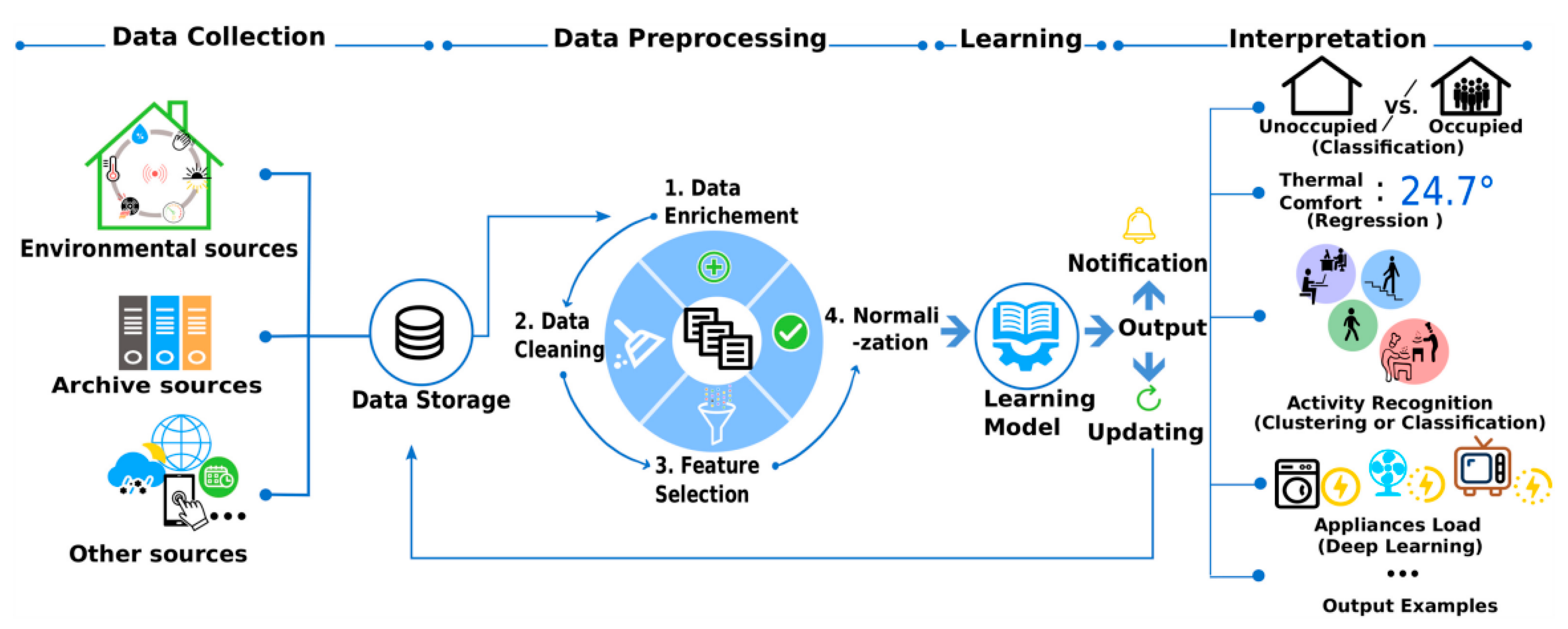
1.1. Data Pre-Processing

Variables influencing total building demand that are sourced from historical databases often experience unpredictable changes and introduce variability [5,6,7]. To address potential inaccuracies and enhance the reliability of results, pre-processing methods are applied prior to machine learning training. A study by D. Djenouri, et al. [8] delineates a standard data pre-processing workflow comprising the following four key steps:

• Data enrichment: dataset enhancement with statistical information.
• Data cleaning: Natural Language Processing (NLP) techniques [9] for textual data.
• Data filtering: elimination of irrelevant features from the dataset, which enhances system efficiency.
• Data normalization: data scaling for accurate comparisons.

Forecasting Performance Criteria

The Mean Absolute Percentage Error (MAPE), Root Mean Square Error (RMSE), and the Mean Absolute Error (MAE) of existing machine learning predictive models are presented in Table 1. The formulas [10] used to calculate these are shown below,

$$MAPE={\displaystyle \frac{1}{n}}\sum _{t=1}^n|{\displaystyle \frac{A-F}{A}}|$$

(1)

$$RMSE=\sqrt{{\displaystyle \frac{{\sum }_{t=1}^n{(A-F)}^2}{n}}}$$

(2)

$$MAE={\displaystyle \frac{{\sum }_{t=1}^n|A-F|}{n}}$$

(3)

where n = summation iteration, A = actual value, and F = forecast value. The MAE value measures the amount of error. The RMSE corresponds to the standard deviation of errors and the MAPE evaluates the effect of the actual values magnitude. For all these metrics, a lower value translates to a more accurate forecasting model [10].

RMSE values often correlate with the magnitude of the actual training and testing data utilized [11]. However, there is a noticeable gap in research regarding the comparison of normalized performance metrics. Refer to Section 2.1 for the calculation of normalized RMSE (nRMSE) figures, where linear regression with 0.864% was identified as the current leading machine learning algorithm in electric load forecasting [12,13].

Table 1. Normalized forecasting performance of machine learning algorithms.

Method	RMSE	nRMSE (%)	Reference
Linear Regression	50.96 MW	0.864	[12]
Compound-Growth	90.76 MW	1.539	[12]
Cubic Regression	98.63 MW	1.673	[12]
ANN	13.3891 kW	3.6995	[13]
SVR-RB	11.6557 kW	3.2205	[13]
SVR-Poly	14.2854 kW	8.2536	[13]
SVR-Linear	15.8223 kW	6.1628	[13]

Table 1. Normalized forecasting performance of machine learning algorithms.

Method	RMSE	nRMSE (%)	Reference
Linear Regression	50.96 MW	0.864	[12]
Compound-Growth	90.76 MW	1.539	[12]
Cubic Regression	98.63 MW	1.673	[12]
ANN	13.3891 kW	3.6995	[13]
SVR-RB	11.6557 kW	3.2205	[13]
SVR-Poly	14.2854 kW	8.2536	[13]
SVR-Linear	15.8223 kW	6.1628	[13]

1.2. Machine Learning Methods for Electric Load Forecasting

Electric load forecasting systems typically utilize past load profile data to predict future consumption, considering factors like weather conditions that display trends in continuous numerical outputs, making regression learning ideal.

Linear regression (LR) is a learning algorithm that aims to find a linear curve solution for predicting continuous outputs. However, its limitation lies in its linearity, which may not be suitable for scenarios requiring more complex relationships between input variables and predicted output. In LR, weight parameters are assigned to training features and iteratively adjusted to minimize errors. Observed data are used to estimate the coefficients that minimize the sum of squared residuals during training. The magnitude and direction of the relationship between each independent and dependent variables are represented by the coefficients. The trained model can then be used to predict new data points by inputting independent variables into the linear Equation (4) [14],

$$h_{\theta }={\theta }_0{+\theta }_1{x}_1+{\theta }_2{x}_2+\dots$$

(4)

where $h_{\theta }$ = predicted output, ${\theta }_n$ = weight parameter, and $x_n$ = training features.

In load forecasting, regression trees enable nonlinear output predictions by dividing data into subsets using nodes, branches, and leaves, minimizing dispersion of target attribute values [15].

Another nonlinear approach is Artificial Neural Networks (ANNs), simulating human brain neurons and adapting to varying consumption trends through backpropagation to minimize errors [16].

Gaussian Process Regression (GPR) models are frequently used in statistical modeling and pattern recognition. These are non-parametric models that employ Gaussian Process, which defines distribution probability over functions, accounting for uncertainty estimates in data predictions.

The covariance function, or kernel, determines the characteristics over functions by defining the relationship between points in the input space. An example below is the exponential kernel Equation (6), which is particularly effective in handling large datasets and achieving smooth functions with minimal errors [17],

$$f\left(x\right)\sim \mathcal{G}\mathcal{P}\left(m\right(x),k(x_i, x_j \left|\theta \right))$$

(5)

$$k(x_i, x_j |\theta )={{\sigma }_f}^2\mathrm{e}\mathrm{x}\mathrm{p}(-{\displaystyle \frac{r}{{\sigma }_l}})$$

(6)

where m(x) = mean function, $r=\sqrt{{\left(x_i-x_j\right)}^T(x_i-x_j)}$, $\theta$ = maximum a posteriori estimate, ${\sigma }_f$ = standard deviation, and ${\sigma }_l$ = length scale.

Training involves kernel hyperparameters learning through the maximization of the marginal likelihood of observed data. Predictions about new data points can then be done through the computation of mean and variance using a calculated covariance matrix from the learned kernel [17].

A general gap identified in previous works is a high variation in performance measures due to differences in limited training datasets. Future improvements involve considering diverse input parameters and exploring hybrid methods for enhanced system forecasting performance.

1.3. Techniques for Machine Learning Optimization

• Optimal Training Data Length (Readings Duration)

Determining the suitable length of past readings for accurate future estimates is crucial in addition to selecting an appropriate model. Research by Y. Chen and Z. Chen [18] revealed that 778 buildings in a dataset exhibited different sensitivities to training data length. For short-term load forecasting (STLF), one year of data proved sufficient due to seasonality impacting weather and occupancy schedules. Interestingly, extending data length up to three years did not significantly enhance STLF accuracy [18].

2.

Parameter Weighting Algorithms for Feature Selection

The presence and continuity of parameters can introduce variations in forecasting accuracy, challenging the notion that more training parameters always lead to improved system performance.

In handling high-dimensional datasets, the Minimum Redundance Maximum Relevance (MRMR) method balances relevance and redundancy by quantifying association measures across all data subsets [19]. It determines variable cardinality by maximizing relevance while avoiding excessive redundancy as expressed in Equation (7) [19],

$$MRMR\left(Xi\right)=max\left[I\left(X_i;Y\right)-{\displaystyle \frac{1}{\left|S\right|}}\sum _{Xj\in S}I(X_i;X_j)\right]$$

(7)

where $I\left(X_i;Y\right)$ = mutual information between feature and target variable (relevance), $I(X_i;X_j)$ = mutual information between features (redundancy), and S = set of selected features.

The F-test evaluates how well a linear regression model fits a dataset compared to a model without predictor variables [20]. Assuming linearity between independent and dependent variables, multivariate normality, and minimal multicollinearity, the F-test determines joint significance among predictors, irrespective of individual variable significance [20],

$$F={\displaystyle \frac{Mean Square Regression}{Mean Square Error}}={\displaystyle \frac{\frac{SSR}{p}}{\frac{SSE}{n-p-1}}}$$

(8)

where SSR = sum of squares due to regression, SSE = sum of squares due to error, p = number of predictors, and n = total number of observations.

Previous studies have favored customized machine learning algorithms tailored to specific datasets. However, diverse dataset sources often present varying forecasting parameters with different recorded lengths. Hence, it is crucial to design a system that offers flexibility across a broader range of datasets. Implemented in MATLAB R2023a, this project addresses the following objectives that structure the rest of the paper:

• Investigate optimal pre-processing methods, training dataset sizes, and automated feature selection methods for enhanced model accuracies.
• Identify the best-performing machine learning algorithm for building and grid electric load forecasting by extensively training and testing with actual electricity consumption readings.
• Develop and integrate building and grid electric load forecasting systems, considering the impacts of local solar PV and electric vehicle (EV) charging, and present findings through an interactive GUI.
• Estimate potential savings of implementing the proposed electric load forecasting system through a case study with verified network stability using industry standard ETAP and Trimble ProDesign software.

2. Methodology

Figure 2 illustrates the implementation workflow undertaken. This involves two separate forecasting models for building and grid applications that were then combined into a single user interface.

2.1. Normalization of Machine Learning Forecasting Performance Measures

Previous studies frequently overlooked normalized performance metrics, restricting the ability to directly compare systems. To identify the most promising methods for deeper investigation, the normalized RMSE figures were calculated using Equation (9). The corresponding values are detailed in

Table 2. List of selected features by parameter weighting.

Method	BDG2 Dataset	UTD Dataset	ERCOT Dataset
MRMR	Air temperature (°C) Sea level pressure (mbar) Dew temperature (°C) Wind direction (degrees) 6 h Precipitation depth (mm)	Hour of day, Day of week, Relative humidity (%), Global horizon irradiance (GHI) (W/m2), Holiday, Solar zenith angle, Dew point (°C Td), Clear sky direct normal irradiance (DNI) (W/m2), Temperature (°C), Wind direction (degrees), Clear sky diffused horizontal irradiance (DHI) (W/m2), DNI (W/m2), Clear sky global horizontal irradiance (GHI) (W/m2), DHI (W/m2)	Temperature (°C) Hour Month Day
F-test	Air temperature (°C) Dew temperature (°C) Sea level pressure (mbar) Wind direction (degrees) Cloud coverage (oktas)	Hour of day, DHI (W/m2), DNI (W/m2), GHI (W/m2), Clear sky DHI (W/m2), Clear sky DNI (W/m2), Clear sky GHI (W/m2), Relative humidity (%), Solar zenith angle, Temperature (°C), Day of week, Dew point (°C Td), Month of year, Day, Wind direction (degrees)	Hour Month Relative Humidity (%) Temperature (°C)

. Notably, linear regression currently exhibits the lowest nRMSE, which corresponds to the best performance at 0.864%.

$$nRMSE={\displaystyle \frac{RMSE}{mean\left(y\right)}}$$

(9)

2.2. Data Collection

Electricity forecasting system performance is dependent on the parameters considered in training and testing. This section lists online sources of real building and electric grid data, providing rationale for dataset selection.

Electric Grid Databases:

• IEEE Data port: Short-Term Load Forecasting using an LSTM Neural Network [21];
• MathWorks File Exchange: Long Term Energy Forecasting with Econometrics in MATLAB [22];
• MathWorks File Exchange: Electricity Load and Price Forecasting Webinar Case Study [23];
• UK National Grid Dataset [24].

Building Demand Databases:

• AMMP Energy Consumption Tracker (Internal BH Record) [25];
• Arizona State University (ASU) Campus Metabolism [26];
• The Building Data Genome 2 (BDG2) Project Data Set [27];
• UCL Smart Energy Research Lab: Energy Use in GB domestic buildings 2021 [28];
• IEEE Data port: Short-Term Load Forecasting Data with Hierarchical Advanced Metering Infrastructure and Weather Features [29].

The application’s requirements include a comprehensive database spanning over a year, reflecting building electricity consumption at the grid level. Consequently, the BDG2 dataset [27], sourced from the UCL Smart Energy Research Lab [28] incorporating the impacts of Electric Vehicle (EV) and Photovoltaic (PV) integration, has been chosen for building electricity forecasting. Texas electric grid data [21], coupled with UTD campus load data [29], were chosen to emulate the case study scenario.

2.3. Pre-Processing

Raw datasets frequently contain missing data and inaccurate outlier readings. Therefore, pre-processing is crucial to transform data and enhance system performance.

The ERCOT dataset [21] comprises hourly electrical demand data spanning from 2012 to 2015. Total demand from served areas—eastern, western, and coastal—was computed to illustrate overall grid capacity and typical demand fluctuations. Additionally, average weather data at each timestamp, encompassing pressure, relative humidity, and temperature, were calculated from three weather stations to mitigate potential discrepancies.

The BDG2 Project dataset [27] and UTD campus load data [29] encompass hourly building meter data readings spanning from 2014 to 2017. The pre-processing techniques applied are summarized as follows:

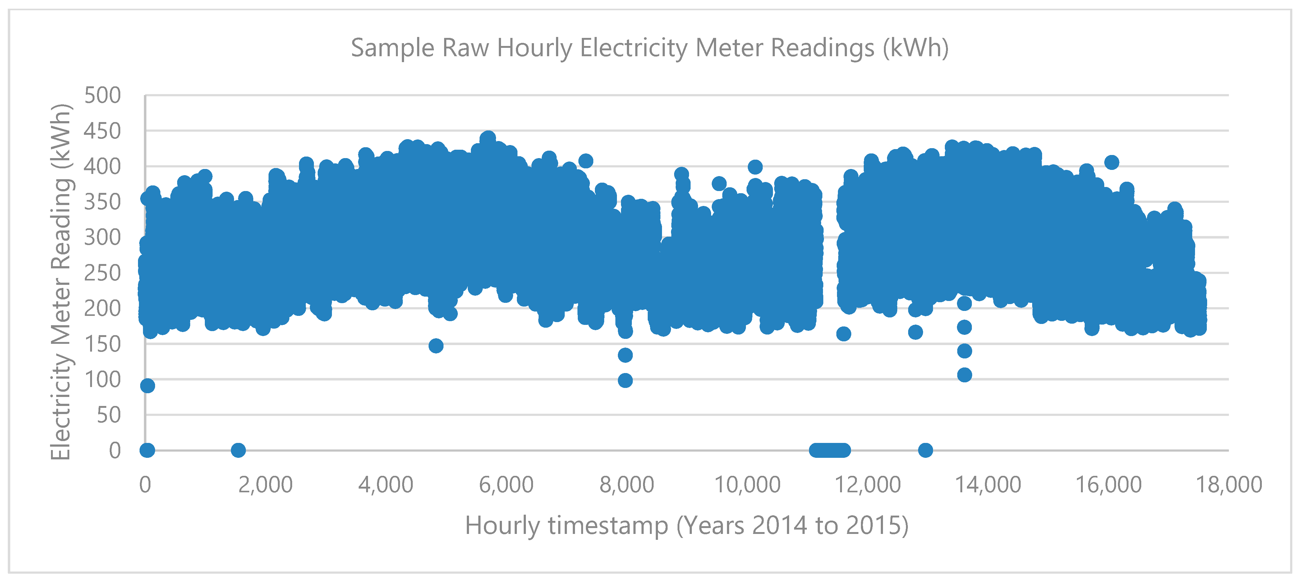
• Identification and removal of data anomalies, such as prolonged streaks of zero values and large positive or negative spikes, were determined through visual inspection. Outlier data were identified using lower and upper bounds calculated from the median and interquartile range (IQR) of differences in consecutive readings, specifically targeting consecutive values with differences greater than 100 kWh.
• Linear interpolation was employed to address missing temperature values.

2.4. Machine Learning (ML) Model Training and Testing

All datasets have been randomly split by 70/30 into training and testing data. This section discusses the machine learning optimization and training methods undertaken to produce the most suitable models for electric grid and building load forecasting purposes.

The MRMR and F-test parameter weighting algorithms were utilized for feature importance ranking and subsequent elimination of ‘negligible’ training parameters. These techniques were implemented on the BDG2 dataset [27], which includes eight weather predictors, and the UTD campus load database [29], comprising twenty predictors. These include external factors that are associated with building energy demand [30]. The same algorithms were also applied to the averaged grid weather data, featuring six predictors, including month and day numbers, hour of the day, average relative humidity, average temperature, and average pressure.

On determining the optimal data size for training, a fixed set of 50,000 data points that was separate from the training data was utilized. The MATLAB ‘randperm’ function was used to procure random data entries without repetition for both building and grid iterations. The normalized RMSE and MAE values were then used to assess the magnitude of change in forecasting performance by varying the dataset sizes used for training.

Most existing load forecasting methodologies heavily rely on trend analysis, predicting future data based on continuous historical figures. To mitigate the negative impacts of events like the COVID-19 pandemic on forecasting accuracy, both training and testing data were organized at random time instances. Various regression algorithms, including linear regression, decision trees, support vector machines (SVMs), and Gaussian Process Regression (GPR), were tested. Each iteration utilized the MATLAB Regression Learner application, and the model with the least error, signifying the highest accuracy, was selected. Multiple iterations of training and testing were conducted on various datasets to ensure system reliability across different data lengths and forecasting variables.

2.5. Building to Grid Interface

The amalgamation of building and grid electric demand forecasting functionalities was presented through an interactive GUI. This enables real-time load forecasting by incorporating weather parameters as user inputs through the deployed trained models.

Additional features include assessing the impact on electricity demand, considering local EV and PV installations. Drawing insights from the UCL Smart Energy Research Lab: Energy use in GB domestic buildings 2021 report [28], the following assumptions were considered:

• Average diurnal values for EV and PV operations represent daily load variations.
• The ratio of the difference to actual values was calculated for each timestamp and applied to the forecasting electric load figure.

3. Results and Validation

3.1. Data Pre-Processing

Figure 3 depicts the impacts of the applied pre-processing techniques in comparison to the corresponding raw sample campus building data showcased in Figure 4. For detailed insights into the quantified effects of pre-processing on model training performance, refer to Section 3.2.3.

3.2. Machine Learning (ML) Model Training and Testing

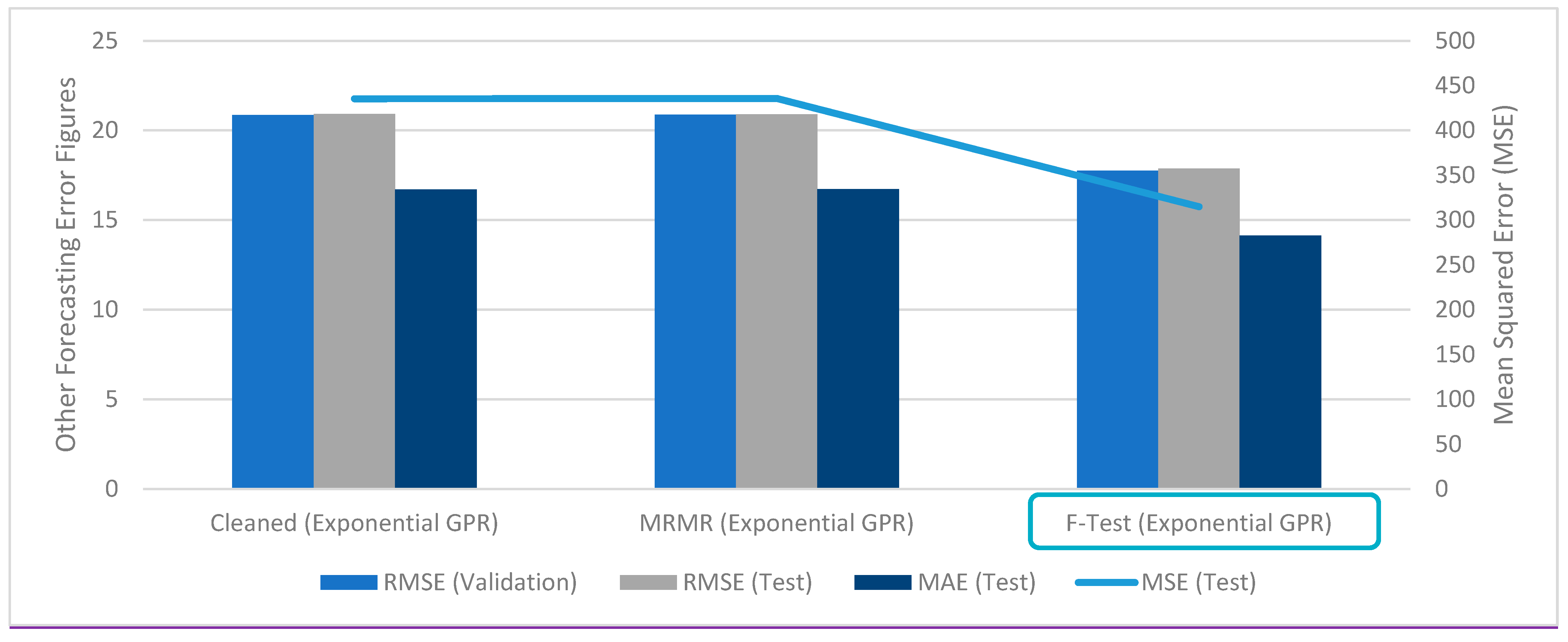
3.2.1. Feature Selection and Parameter Weighting

Utilizing MRMR and F-test feature selection methods across various databases, Table 2 presents the selected features ranked by importance based on the applied method. The decision-making criteria for determining the number of ‘relevant’ features are outlined as follows:

• BDG2 building dataset [27]—Opting for the top five out of eight features, with consideration given to the sixth feature’s score being less than 50% of the fifth feature.
• UTD campus load data [29]—Selection of the top fifteen out of twenty features, ensuring that the score of the sixteenth feature is less than 70% of the fifteenth feature.
• ERCOT grid data [21]—Choosing the top four out of six features, with consideration given to the fifth feature’s score being less than 50% of the fourth feature, or the top four features having an ‘infinite’ F-test score.

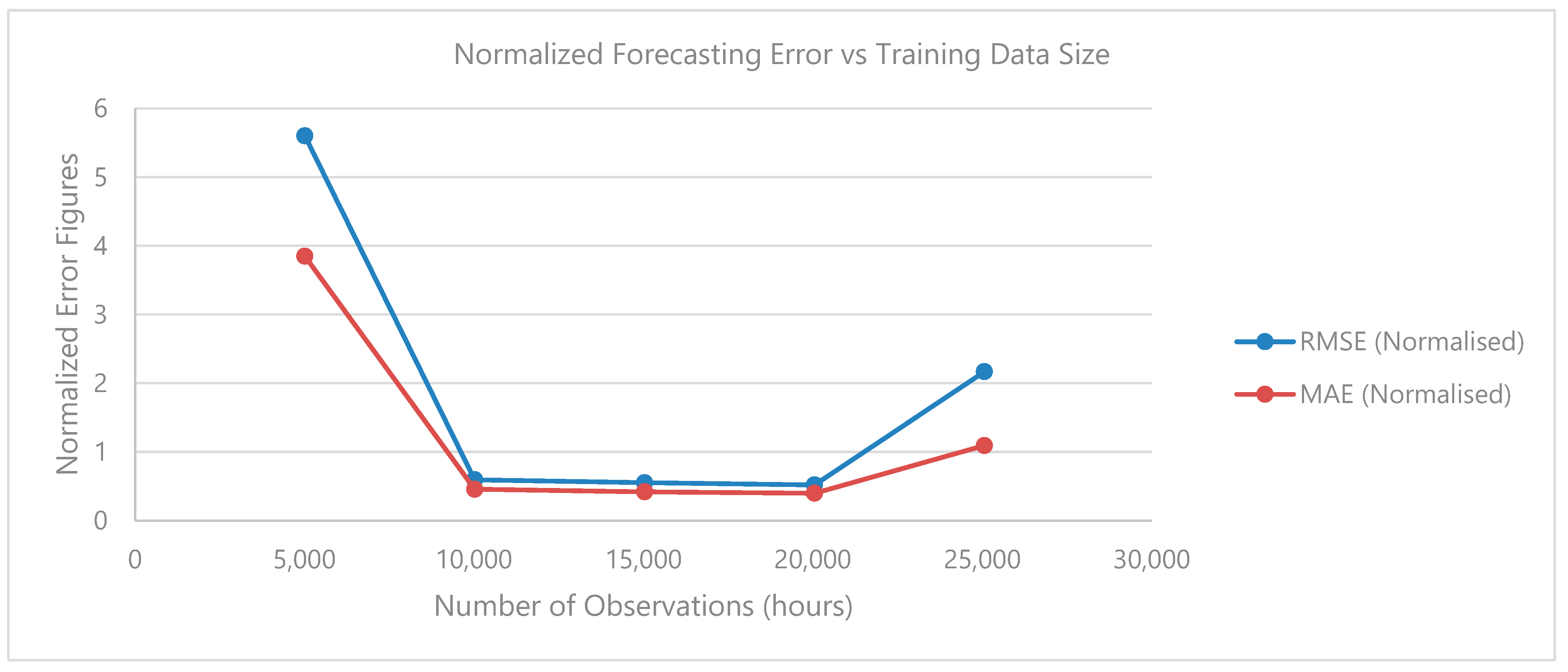
3.2.2. Optimal Training Data Duration

The determination of the optimal training data duration involved assessing calculated normalized RMSE and MAE values. Through iterative tests covering a range of grid electricity demand observations used as training data (from 5000 to 25,000 h), testing data were randomly selected from a pool of 35,065 data points.

The recorded forecasting errors reached their maximum within the first 10,000 h due to insufficient training data. Consistent with findings in published studies [18], the lowest normalized errors were observed when the training data covered at least 1 year of hourly readings, as depicted in Figure 5. Notably, beyond 2.3 years of data, errors increased due to heightened risks of model complexity and overfitting, as corroborated by similar results obtained from building electricity demand databases [31].

3.2.3. Forecasting Model Training and Selection

As mentioned in Section 2, various machine learning regression algorithms outlined in

Table 3. List of machine learning algorithms tested.

List of Machine Learning Algorithms (MATLAB Regression Learner)
Linear Regression Models Linear, Interactions Linear, Robust Linear, Stepwise Linear Regression Trees Fine Tree, Medium Tree, Coarse Tree Support Vector Machines Linear SVM, Quadratic SVM, Fine Gaussian SVM, Medium Gaussian SVM, Coarse Gaussian SVM	Gaussian Process Regression (GPR) Rational Quadratic GPR, Squared Exponential GPR, Matern 5/2 GPR, Exponential GPR Kernel Approximation Regression SVM Kernel, Least Squares Kernel Regression Ensembles of Trees Boosted Trees, Bagged Trees Neural Networks (NN) Narrow NN, Medium NN, Wide NN, Bi-layered NN, Tri-layered NN

were employed for model training. The subsequent summary of results quantifies the impacts of diverse optimization measures on the forecasting accuracies of averaged samples from building and grid data. The system combinations yielding the lowest error figures, and consequently the most accurate results, were selected and applied to the case study scenario.

The results in Figure 6 and Figure 7 suggest that Exponential GPR consistently outperformed the other listed algorithms in both building and grid-level electric demand forecasting applications. Please refer to Section 4.2 for details on Exponential GPR algorithm characteristics that led to the acquisition of the presented results.

By applying Equation (6), the normalized RMSE value for the chosen model was computed as 0.52%, obtained by dividing RMSE (Test) by the average forecasted figure. This represents approximately a 0.3% enhancement compared to the existing leading linear regression methodology, which has an nRMSE of 0.864% [12].

For further results validation, the same optimization and model training methodology was applied using data collected from a residential building located in Eastern USA [27]. A summary of results is presented in Figure 8, noting consistent outperformance of exponential GPR, which yielded a calculated nRMSE of 0.59% over other algorithms for load demand forecasting in a sample building with varying usage and location.

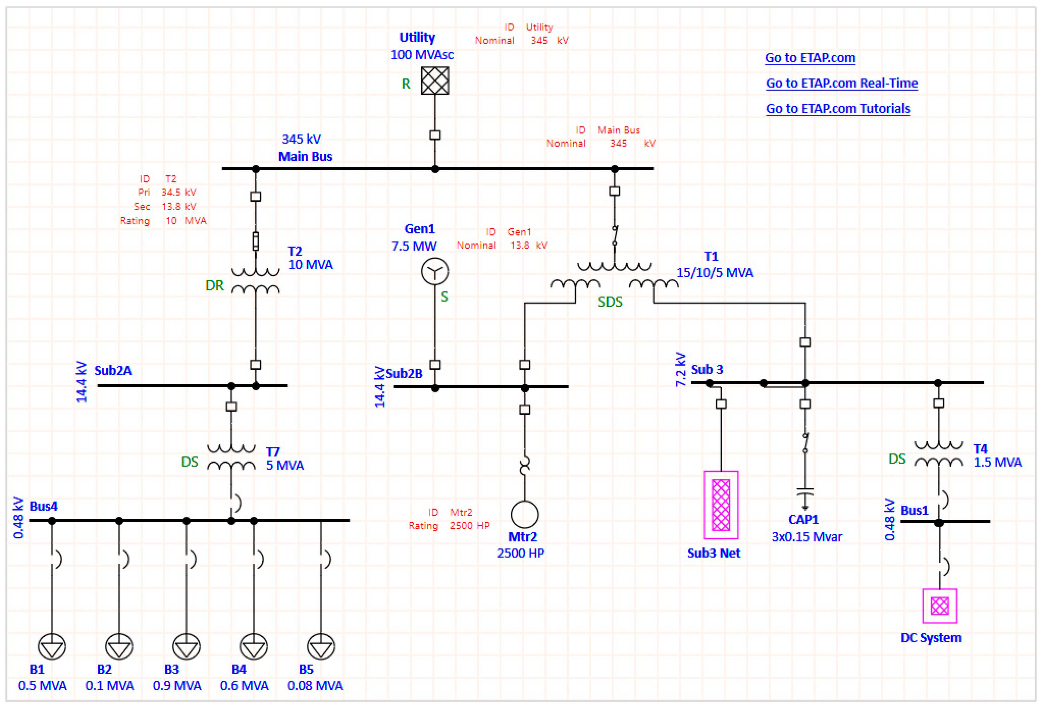
3.3. Case Study Verification

The case study scenario was configured with voltage parameters in Texas, USA, after confirming the alignment of weather data between the UTD [29] and ERCOT [21] databases. The high-voltage system distribution network was established in ETAP 22 software, as illustrated in Figure 9, with the following characteristics:

• A 100 MVA utility supply in accordance with Texas western electric grid capacity [32].
• Texas transmission lines energized at 7.2 kV or 14.4 kV, subsequently lowered to 480 V via transformers [33].

The design was input into Trimble ProDesign to validate the stability of the low-voltage system at peak full load as shown in Figure 10. This comprehensive simulation ensures that parameters such as voltage drops are well within industry limits to confirm applicability of the case study to real-world scenarios for accurate energy savings estimation.

Calculations were based on the listed assumptions below.

• One MV/LV transformer feeds five campus buildings within the same plot.
• Equal distances between the MV/LV transformer and campus buildings were considered.
• All campus buildings were modeled as ‘lump loads’ based on the maximum loads recorded from the UTD database [29] plus a 10% spare.
• All demand loads were applied with a power factor of 0.8 and a frequency of 60 Hz.

3.4. System Savings Estimation

3.4.1. Electric Vehicle (EV) Local Forecasting Savings

The report data [28] indicate that EV ownership leads to an increase in average electricity consumption, primarily due to charging. Typically, forecasting savings are derived from peaks in demand variation. To quantify the peak values in kW exclusively, the minimum difference between the ‘with EV’ and ‘without EV’ curves was subtracted from the average difference. This yields a potential savings ratio of 14.7% from the maximum load, as outlined in

Table 4. EV ownership forecasting savings estimation.

Minimum difference (with EV − without EV)	0.147 kW
Average difference − minimum difference	0.145 kW
Peak load (worst-case scenario)	0.984 kW
Calculated savings ratio (0.145/0.984)	14.7%

.

3.4.2. Solar Photovoltaic (PV) Local Forecasting Savings

Decreases in external electricity consumption resulting from photovoltaic (PV) systems can be identified during midday when panel outputs reach their maximum. To calculate savings attributed to PV systems forecasting, it is assumed that PV output durations are known. Therefore, only instances where buildings with PV installations consumed more electricity than their counterparts without (indicated by a positive difference) were taken into consideration, resulting in potential electricity savings of up to 12.9% (

Table 5. PV ownership forecasting savings estimation.

Average of +ve difference	0.079 kW
Peak load (worst-case scenario)	0.612 kW
Calculated savings ratio (0.079/0.612)	12.9%

).

3.4.3. Combined System Electricity Demand Forecasting Savings

The values presented in

Table 6. Combined system forecasting savings estimation.

	Smart Building	Smart Grid
Variance	3228.4 kW2	81,314,603.5 kW2
Standard Deviation	56.82 kW	9017.5 kW
Estimated Savings	9.35%	11.47%
Estimated Savings with Local EV/PV Installations	11.93%	N/A

comprise aggregated data from the performances of the selected smart building and smart grid forecasting models along with the estimated local savings from electric vehicle (EV) and photovoltaic (PV) ownership. To gauge trend variation in building and grid electricity demand, standard deviation figures were computed, serving as indicators of potential savings with effective forecasting. Estimated savings were then calculated using Equation (10), factored with the identified model nRMSE figures, which measure the normalized average magnitude of error.

$$Estimated Savings={\displaystyle \frac{Standard deviation}{Average demand}}\ast (1-nRMSE)$$

(10)

The accuracy of final loads, such as building demand, influences the performance of grid forecasting. When applied as a factor of the estimated smart grid savings, this percentage (11.93%) contributes to a combined system electricity demand forecasting saving of 12.8% from the grid perspective.

Considering the following rates for Texas, USA, the annual estimated case study savings, assuming all outgoing connections from the grid adopt forecasting systems, were calculated as USD 277,682.7 and 1,090,638.11 kgCO₂. It is important to note that additional savings from local incentives were not factored into these estimates.

• Texas electricity rate (August 2023) = 0.1136 USD/kWh [34].
• Texas generation factor = 0.44618 kgCO₂/kWh [35].

3.5. Graphical User Interface (GUI) Integration

Figure 11 displays a screenshot of the interactive GUI created for the building classification system using MATLAB. Users are prompted to enter building characteristics and forecasted weather data, which are then used to predict the final electric load in kW. Additional functionalities related to the case study are presented in separate tabs within the GUI window.

For existing buildings with pre-recorded readings, identification of ‘closest match’ from external database is not required. Predicted weather data can be automatically imported from the source to eradicate risks of human error. Likewise, predicted building electric demand load figures can be shared directly to the power grid system and vice versa for effective demand management.

4. Discussion

4.1. Regression Model Training Optimization

MSE, MAE, and RMSE served as performance metrics for all model training and testing iterations. While all three metrics indicate better accuracy with lower values, (normalized) RMSE was the primary deciding factor for model comparison. This choice was influenced by the following reasons:

• RMSE figures are commonly available in previously published papers, facilitating direct comparisons between model performances.
• The RMSE formula squares the prediction difference, highlighting larger differences and representing the worst-case forecasting figure.
• RMSE is equivalent to the mathematical standard deviation of residuals, providing an average difference between predicted and actual values, useful for determining system accuracy.

The applied pre-processing methods, including optimal training dataset size investigation and automated feature selection, led to the following conclusions:

• Optimal training dataset size for reduced errors and preventing model overfitting is approximately 1–2 years’ worth of hourly data. Beyond this, there is a risk of model generalization, characterized by low training RMSE and high testing RMSE.
• Feature selection methods like MRMR and F-test rank training variables by importance. It is important to note that not all models benefit from limiting the quantities of training variables, and it is recommended to conduct feature selection for each new database.
• Improvement percentages for RMSE, MSE, and MAE using combined methods averaged at 12.34%, 24.40%, and 9.1% for building-level electric demand forecasting.

4.2. Exponential GPR for Electric Load Forecasting

In numerous iterations of forecasting models, the Exponential Gaussian Process Regression (GPR) algorithm stands out for minimizing calculated errors. Although its prevalence in load forecasting has not been extensively explored, its improved performance can be attributed to the following specific algorithm characteristics [17]:

• Non-parametric: it makes no assumptions about the entire data population based on the sample training dataset. Algorithms in this category often demonstrate higher robustness with datasets featuring large distribution measures.
• Bayesian approach: it applies a probability distribution over all possible values, enabling the provision of predictions with uncertainty measurements.
• Exponential GPR kernel: this feature facilitates effective handling of large datasets. When combined with the described pre-processing methods, smooth functions can be achieved with minimal errors.

Typical forecasting algorithms rely on trend recognition to continue the demand curve based on previous values. The implemented method in this study considers randomized data inputs, allowing for enhanced flexibility in forecasting. By minimizing reliance on trends and maximizing the impact of ‘relevant’ variables, higher forecasting accuracies can be achieved. This approach provides more control over extreme variations caused by external events, such as the COVID-19 pandemic, which could potentially lead to significant dips or peaks in demand.

4.3. Case Study Verification and Savings Estimation

The assumptions made for the impact study of local solar PV and EV systems are tied to the calculation of building-level demand savings resulting from forecasting. For example, the UCL Energy Report database, while useful for assessing average system impacts, may likely subdue high peaks and variations due to its representation of averaged meter readings from multiple sources. Additionally, differences in lifestyles and corresponding power demands between households with EV and PV systems and those without contribute to the observed variation. This explains the existence of demand differences during periods when these systems are inactive.

Modeling the case study scenario in ETAP and Trimble ProDesign instills confidence in determining the stability of the system while exhibiting peak steady-state loads. In this defined scenario, the overall electricity savings when viewed from the grid-side was found to be 12.8%. This assumption is based on the full standard deviation minus the nRMSE factors, representing energy savings due to forecasting in cases where previous manual forecast figures and carbon levies are unavailable.

4.4. Recommendations

The increasing flexibility and reliability of machine learning capabilities have garnered widespread adoption across various applications. The implementation of regression forecasting demands minimal equipment costs, with most expenses associated with system development and maintenance.

Table 7. System requirements for new and existing buildings.

System Requirements	New Buildings	Existing Buildings
Electricity consumption meter	✓	Often available through the incoming supply to building.
Recording and storage of new consumption data	✓	✓
Access to equivalent previous data recordings	✓	Previous data recordings assumed to be available.
Annual model recalibration with new training data	✓	✓
Information share with grid	✓	✓

provides a summary of the deployment requirements for both new construction and existing buildings.

It should be noted that in the absence of actual historical data, previous data recordings from a building of similar scale, usage, and location may likewise be considered for existing buildings. Considering that recorded data types may vary between different buildings, it is recommended to perform feature selection by parameter weighing for each new dataset to accurately identify features that would enhance forecasting performance. Another challenge may be caused by irregular data recording timestamps. Regular frequency of data recordings is essential in pattern recognition. Hence, in such cases data shall be pre-processed such that recording frequencies are maintained by limiting model inputs as per the largest (worst-case) timestamp interval.

The costs associated with the specified requirements can vary significantly based on the scale of deployment. For instance, storage of consumption data may be centralized or local, with the latter potentially incurring cloud subscription fees through Building Management Systems (BMSs). Similarly, the aggregate manpower needed to train and recalibrate local building consumption forecasting models is likely to be higher if done locally compared to a centralized approach.

The primary setup costs are associated with data scientist/engineer manpower for tasks such as data collection, model training, and optimization. Following the defined methodology, this process takes approximately 6 h at an average rate of USD 61 per hour [36]. It is important to note that this is a minimum estimate, and additional costs may arise if any of the following assumptions vary for each scenario:

• Availability of building data storage through an existing BMS.
• Possession of an existing MATLAB (or similar) software license.
• Full access to previous and forecasted local weather data.
• Annual model recalibration to include past-year data.

Model recalibration is recommended using past-year data to allow gradual performance enhancement by essentially learning from previous accuracies. This process requires a data scientist/engineer to retrain the model if required through a thorough evaluation of previous forecasting performance, leading to error reduction. The existing forecasting model is able to operate as normal during this process which can then be replaced by the recalibrated model between reading intervals to avoid service interruptions.

Similar resources are required for grid electric demand forecasting. Full collaboration and usage transparency from both the grid and consumers are essential for frequent model recalibrations, maximizing potential savings.

4.5. Conclusions and Future Work

This research comprehensively addressed various aspects of electric demand load forecasting, encompassing optimization, machine learning algorithm selection, and testing through simulations. However, like other simulated studies, there is room for improvement and further exploration through real-world applications. Potential areas for investigation include the following:

• System implementation in operational buildings. Involving regular performance assessments to gauge its effectiveness in real-world scenarios.
• Expanded database sources. Using additional database sources to further validate and enhance the obtained results.
• Integration effects of external systems. Investigating the integration effects of other external systems on building electric demand to understand how various factors influence forecasting accuracy.
• Study on different generation technologies. Conducting a detailed study on the effects of different types of generation panels and capacities on overall building and grid demand to optimize energy generation.
• Extended applications of load forecasting. Exploring the implementation of load forecasting on extended areas of research such as information exchange security and larger-scale renewable energy generation.

References

1. Kolokotsa, D. The role of smart grids in the building sector. Energy Build. 2015, 116, 703–708. [Google Scholar] [CrossRef]
2. Schito, E.; Lucchi, E. Advances in the Optimization of Energy Use in Buildings. Sustainability 2023, 15, 13541. [Google Scholar] [CrossRef]
3. Buro Happold. Digital Buildings Consultancy Presentation, 2021.
4. Wurtz, F.; Delinchant, B. “Smart buildings” integrated in “smart grids”: A key challenge for the energy transition by using physical models and optimization with a “human-in-the-loop” approach. Comptes Rendus Phys. 2017, 18, 428–444. [Google Scholar] [CrossRef]
5. Martín-Lopo, M.; Boal, J.; Sánchez-Miralles, Á. A literature review of IoT energy platforms aimed at end users. Comput. Netw. 2020, 171, 107101. [Google Scholar] [CrossRef]
6. Xie, X.; Lu, Q.; Herrera, M.; Yu, Q.; Parlikad, A.; Schooling, J. Does historical data still count? Exploring the applicability of smart building applications in the post-pandemic period. Sustain. Cities Soc. 2021, 69, 102804. [Google Scholar] [CrossRef] [PubMed]
7. Wang, Z.; Srinivasan, R. A review of artificial intelligence-based building energy use prediction: Contrasting the capabilities of single and ensemble prediction models. Renew. Sustain. Energy Rev. 2017, 75, 796–808. [Google Scholar] [CrossRef]
8. Djenouri, D.; Laidi, R.; Djenouri, Y.; Balasingham, I. Machine Learning for Smart Building Applications. ACM Comput. Surv. 2020, 52, 1–36. [Google Scholar] [CrossRef]
9. Yi, J.; Nasukawa, T.; Bunescu, R.; Niblack, W. Sentiment analyzer: Extracting sentiments about a given topic using natural language processing techniques. In Proceedings of the Third IEEE International Conference on Data Mining, Melbourne, FL, USA, 22 November 2003; pp. 427–434. [Google Scholar] [CrossRef]
10. Klimberg, R.K.; Sillup, G.P.; Boyle, K.J.; Tavva, V. Forecasting performance measures—What are their practical meaning? Adv. Bus. Manag. Forecast. 2010, 7, 137–147. [Google Scholar] [CrossRef]
11. Jedox. Error Metrics: How to Evaluate Your Forecasting Models. Available online: https://www.jedox.com/en/blog/error-metrics-how-to-evaluate-forecasts/#nrmse (accessed on 14 June 2023).
12. Samuel, I.A.; Emmanuel, A.; Odigwe, I.A.; Felly-Njoku, F.C. A comparative study of regression analysis and artificial neural network methods for medium-term load forecasting. Indian J. Sci. Technol. 2017, 10, 1–7. [Google Scholar] [CrossRef]
13. Alrashidi, A.; Qamar, A.M. Data-driven load forecasting using machine learning and Meteorological Data. Comput. Syst. Sci. Eng. 2021, 44, 1973–1988. [Google Scholar] [CrossRef]
14. Varghese, D. Comparative Study on Classic Machine Learning Algorithms. Medium. Available online: https://towardsdatascience.com/comparative-study-on-classic-machine-learning-algorithms-24f9ff6ab222 (accessed on 18 June 2023).
15. Regression Trees. IBM Documentation. Available online: https://www.ibm.com/docs/en/db2-warehouse?topic=procedures-regression-trees (accessed on 18 June 2023).
16. Rouse, M.; Artificial Neural Network. Techopedia. Available online: https://www.techopedia.com/definition/5967/artificial-neural-network-ann (accessed on 18 June 2023).
17. Zhang, N.; Xiong, J.; Zhong, J.; Leatham, K. Gaussian process regression method for classification for high-dimensional data with limited samples. In Proceedings of the 2018 Eighth International Conference on Information Science and Technology (ICIST), Cordoba, Granada, and Seville, Spain, 30 June–6 July 2018. [Google Scholar] [CrossRef]
18. Chen, Y.; Chen, Z. Short-term load forecasting for multiple buildings: A length sensitivity-based approach. Energy Rep. 2022, 8, 14274–14288. [Google Scholar] [CrossRef]
19. Berrendero, J.R.; Cuevas, A.; Torrecilla, J.L. The MRMR Variable Selection Method: A Comparative Study for Functional Data. J. Stat. Comput. Simul. 2015, 86, 891–907. [Google Scholar] [CrossRef]
20. Sureiman, O.; Mangera, C. F-test of overall significance in regression analysis simplified. J. Pract. Cardiovasc. Sci. 2020, 6, 116. [Google Scholar] [CrossRef]
21. Hossain, M.S.; Mahmood, H. Data Set Used in the Conference Paper Titled “Short-Term Load …”. IEEE DataPort. Available online: https://ieee-dataport.org/documents/data-set-used-conference-paper-titled-short-term-load-forecasting-using-lstm-neural (accessed on 29 July 2023).
22. Willingham, D. Long Term Energy Forecasting with Econometrics in MATLAB. MATLAB Central File Exchange. 2023. Available online: https://www.mathworks.com/matlabcentral/fileexchange/49279-long-term-energy-forecasting-with-econometrics-in-matlab (accessed on 22 January 2023).
23. Deoras, A. Electricity Load and Price Forecasting Webinar Case Study. MATLAB Central File Exchange. 2023. Available online: https://www.mathworks.com/matlabcentral/fileexchange/28684-electricity-load-and-price-forecasting-webinar-case-study (accessed on 22 January 2023).
24. Datasets. National Grid’s Connected Data Portal. Available online: https://connecteddata.nationalgrid.co.uk/dataset/?groups=demand (accessed on 29 July 2023).
25. Buro Happold. AMMP Energy Consumption Tracker April 2022 Data, 2022.
26. Campus Metabolism. Arizona State University—Campus Metabolism. Available online: https://sustainability-innovation.asu.edu/campus/what-asu-is-doing/ (accessed on 30 July 2023).
27. Miller, C.; Biam, P. The Building Data Genome 2 (BDG2) Data-Set. GitHub. Available online: https://github.com/buds-lab/building-data-genome-project-2 (accessed on 30 July 2023).
28. Pullinger, M.; Few, J.; McKenna, E.; Elam, S.; Oreszczyn, E.W.T. Smart Energy Research Lab: Energy Use in GB Domestic Buildings 2021 (Volume 1)—Data Tables (in Excel). University College London, 13 June 2022. Available online: https://rdr.ucl.ac.uk/articles/dataset/Smart_Energy_Research_Lab_Energy_use_in_GB_domestic_buildings_2021_volume_1_-_Data_Tables_in_Excel_/20039816/1 (accessed on 29 July 2023).
29. Zhang, J. Short-Term Load Forecasting Data with Hierarchical Advanced Metering … IEEE Data Port. Available online: https://ieee-dataport.org/documents/short-term-load-forecasting-data-hierarchical-advanced-metering-infrastructure-and-weather (accessed on 29 July 2023).
30. Najini, H.; Nour, M.; Al-Zuhair, S.; Ghaith, F. Techno-Economic Analysis of Green Building Codes in United Arab Emirates Based on a Case Study Office Building. Sustainability 2020, 12, 8773. [Google Scholar] [CrossRef]
31. Lusis, P.; Khalilpour, K.R.; Andrew, L.; Liebman, A. Short-term residential load forecasting: Impact of calendar effects and forecast granularity. Appl. Energy 2017, 205, 654–669. [Google Scholar] [CrossRef]
32. ERCOT. March Report to ROS—Electric Reliability Council of Texas. Available online: https://www.ercot.com/files/docs/2017/03/29/14._SSWG_Report_to_ROS_March_2017_R2.docx (accessed on 12 July 2023).
33. Texas Co-Op Power. Field Guide to Power Lines. Available online: https://texascooppower.com/field-guide-to-power-lines/#:~:text=Distribution%20Lines&text=These%20lines%20are%20energized%20at,residential%20homes%20and%20small%20businesses (accessed on 12 July 2023).
34. Electric Choice. Electric Rates. Available online: https://www.electricchoice.com/electricity-prices-by-state/ (accessed on 7 August 2023).
35. Carbon Footprint. Country Specific Electricity Grid Greenhouse Gas Emission Factors. Available online: https://www.carbonfootprint.com/docs/2020_07_emissions_factors_sources_for_2020_electricity_v1_3.pdf (accessed on 7 August 2023).
36. ZipRecruiter. Salary: Data Scientist (June 2023) United States. Available online: https://www.ziprecruiter.com/Salaries/DATA-Scientist-Salary (accessed on 18 August 2023).
Figure 1. A general framework of machine learning solutions [5].
Sustainability 16 08752 g001
Figure 2. Building and grid electric load forecasting implementation workflow.
Sustainability 16 08752 g002
Figure 3. Cleaned hourly electricity meter readings (kWh) of a sample campus building.
Sustainability 16 08752 g003
Figure 4. Raw hourly electricity meter readings (kWh) of a sample campus building.
Sustainability 16 08752 g004
Figure 5. Iterative test for identification of optimal training data duration.
Sustainability 16 08752 g005
Figure 6. Averaged building electric demand forecasting errors.
Sustainability 16 08752 g006
Figure 7. Averaged grid electric demand forecasting errors.
Sustainability 16 08752 g007
Figure 8. Residential building electric demand forecasting errors.
Sustainability 16 08752 g008
Figure 9. Case study distribution network model using ETAP software (ETAP.com).
Sustainability 16 08752 g009
Figure 10. Low voltage network stability test using Trimble ProDesign version 2021.0.19.
Sustainability 16 08752 g010
Figure 11. Building classification MATLAB GUI.
Sustainability 16 08752 g011