Aeromagnetic Data Analysis for Sustainable Structural Mapping of the Missiakat Al Jukh Area in the Central Eastern Desert: Enhancing Resource Exploration with Minimal Environmental Impact

Abstract

This study integrates aeromagnetic data with geological information to develop a consistent interpretation of both shallow and deep structural frameworks at various depths in the Missiakat Al Jukh area, located in the Central Eastern Desert, Egypt. The research begins by processing reduced-to-the-north magnetic pole (RTP) anomalies, using Fast Fourier Transformation (FFT) techniques to distinguish between local residual structures and broader regional features. This multi-scale approach enables a more detailed understanding of the geological complexity in the region, revealing its subsurface structures. Advanced geophysical methods such as upward continuation, Euler deconvolution, source parameter imaging (SPI), and global particle swarm optimization (GPSO) were applied to further refine the determination of structural depths, offering critical insights into the distribution and orientation of geological features at varying depths. The study reveals dominant structural orientations aligned in the NNW-SSE, ENE-WSW, north–south, and east–west directions, reflecting the region’s complex tectonic history. This research is of great importance in terms of sustainability. By delivering detailed subsurface maps and providing more accurate depth estimates of basement rocks (between 0.6 and 1.3 km), it contributes to sustainable resource exploration in the region. A better understanding of the geological structure helps minimize the environmental impact of exploration by reducing unnecessary drilling and concentrating efforts on areas with higher potential. Additionally, the use of non-invasive geophysical techniques supports the transition toward more environmentally conscious exploration practices. The integration of these advanced methods promotes a more sustainable approach to mineral and resource extraction, which is crucial for balancing economic growth with environmental preservation in geologically sensitive areas. Ultimately, this work provides a thorough geological interpretation that not only aids future exploration efforts but also aligns with the global push for sustainable and eco-friendly resource management.

1. Introduction

The tectonic development of the Eastern Desert is strongly influenced by the interaction between major shear zones and secondary structures, formed within a strike-slip regime. This includes the synthetic Riedel (R) shears and the antithetic R’ shears, as well as en-echelon structures linked to localized extension or compression [1,2]. These shear zones and associated subsidiary structures often act as conduits for fluid flow, potentially giving rise to magnetic anomalies. The concentration of strain along these features can create dilatational zones, which are favorable environments for mineralization.

The studied area lies within Egypt’s Central Eastern Desert (Figure 1) and is positioned between latitudes 26°17′ to 26°38′ N and longitudes 33°15′ to 33°52′ E. The study area covers approximately 240,000 km² and features steep to rugged topography. It is crisscrossed by numerous Wadis (dry valleys) that primarily run in the NE-SW, NW-SE, WNW, and E-W directions, including Wadi (W.) Al-Markh, W. Bulah, W. Missikat AL-Jukh, and W. Al-Jidami. Numerous landmarks are present within the study area, including Jabal (J.) Missiakat AL-Jukh, J. Rie Al-Jarrah, J. Maghrabiyah, J. Urf Salih, J. Um Halham, J. Wash, and J. Al-Jidami.

The study area predominantly comprises igneous, metamorphic, and sedimentary rocks, spanning from the Precambrian to the Quaternary era (Cenozoic). The Egyptian Geological Survey and Mining Authority (EGSMA) [3] conducted a surface geology mapping of this region in 1992. This mapping initiative commenced with the identification of epidote chlorite metabasic schist from the Precambrian era and delineation of Wadi sediments from the Quaternary era (Figure 2). Regarding topography, the studied area features low hills alongside high and rugged mountains. Stratigraphically, it is overlaid with a diverse range of basement and sedimentary rocks. Precambrian rocks cover most of the study area in the northeastern, northwestern, central, and southwestern parts. These rocks consist of biotite alkali granite (gk), monzogranite (gm), granodiorite (gd), xenolithic granodiorite (gt), hornblende gabbro and diorite (gbd), hornblende monzodiorite (gb), chert rhyolite (vpc), rhyolite and dacite (va), andesite (vib), ferrobasaltic and dolerite (vb), metavolcanic schist (omv), massive hornblende gabbro (ohgb), erpentinite (osm), amphibolite, Hammamat sediments (ha), Dukhan volcanics (dk), chlorite, quartz, and talc schist (mv), as well as Epidote and chlorite metabasic schist (mvb). The study area’s southeastern, northwestern, and western portions are covered by clastic sedimentary rocks from the Upper Cretaceous, represented by the Dokhan (kuda) and Tarif (kut) formations. Oligocene sedimentary rocks, predominantly sandstone, are found sporadically in the study site’s northwestern and central western areas, characterized by the Nakhil (ton) Formation [4]. Quaternary Wadi sediments are present in the study area’s southeastern, southwestern, and northern regions. Figure 2 depicts various dykes with different orientations, including NNE-SSE, NW-SE, and WNW-ESE, located in the eastern part of the study area [3].

Structurally, the investigated area underwent various tectonic movements, resulting in the formation of intricate structures. It is traversed by several faults and joints, which either coincide with Wadis (drainage lines) or traverse the country rocks (Figure 2). These faults primarily trend in the NNW-SSE, ENE-WSW, and N-S directions, with some minor faults trending in the E-W direction [5,6,7]. This study aims to identify and recognize the contact zones among different types of rocks and the structural lineaments that dissect shallow and deep sections of the area under investigation using aeromagnetic data. Aeromagnetic data are utilized in various earth science disciplines, including energy exploration (geothermal and fossil fuels), hydrology, archaeology, mining, and imaging subsurface structures [8,9,10,11,12,13]. Our work offers a comprehensive geological interpretation that supports this global push for sustainable and environmentally friendly resource management while also assisting future exploratory efforts.

2. Materials and Methods

In 1984, the Aero-Service Division of Western Geophysical Company of America [14] conducted an aerial geophysical survey in the designated study area, part of the Eastern Desert of Egypt. Aeromagnetic surveys were carried out with flight lines running parallel in the NE-SW direction, which were positioned nearly perpendicular to the overall alignment of the Red Sea, spaced at intervals of 1.5 km. Additionally, tie lines were flown at intervals of 10 km in the NW-SE direction.

2.1. Reduction to the North Magnetic Pole (RTP)

To minimize the impact of the Earth’s magnetic field inclination on the shapes, sizes, and locations of anomalies, aeromagnetic data underwent a reduction to the North Magnetic Pole [15,16]. This reduction facilitated a more precise assessment of magnetized sources and the identification of significant magnetic zones displaying uncommon amplitudes and gradient anomalies. The magnetic data analysis began by converting the total aeromagnetic intensity map (Figure 3) to the North Magnetic Pole (where I = 90° and D = 0°), thereby removing the influence of Earth’s magnetic field inclination and declination from the dataset. This reduction was carried out using the Oasis Montaj™ software version 7.1, [17]. Consequently, all anomalies in the resulting RTP magnetic map closely correspond to the locations of the sources as referenced by (Baranov and Naudy [18], Baranov [19] and Bhattacharyya (1965 and 1967)) [20,21] (Figure 4).

2.2. Spectral Frequency Analysis

Filtering techniques, such as residual/regional separation, were utilized to identify the shallow and deep sources accountable for residual and regional fields. The aeromagnetic data can be depicted through a 2D Fourier series comprising diverse frequencies, enabling the characterization of existing anomalies [22,23,24]. In this study, we utilized Fast Fourier Transform (FFT) to analyze the RTP aeromagnetic survey data, allowing us to calculate their energy spectrum. This process generated a 2D power spectrum curve (Figure 5). This curve was divided into two components based on the spectrum’s characteristics, namely, alterations in the slope of the curve: the regional (deep-seated) component, which mainly influences the long-wavelength or low-frequency part of the spectrum, and the residual (shallow) component, which mainly affects the short-wavelength or high-frequency or segment (Ogunmola et al. 2016; Salawu et al., 2019a,b) [9,10].

The Gaussian filter method was used to separate the RTP aeromagnetic data in the studied region, relying on the energy spectrum analysis results of the aeromagnetic data. Residual and regional magnetic anomalies were produced for the two specified boundaries (refer to Figure 6 and Figure 7), respectively. The residual anomaly highlights less prominent features that are masked by the dominant regional effects visible in the RTP aeromagnetic map [25].

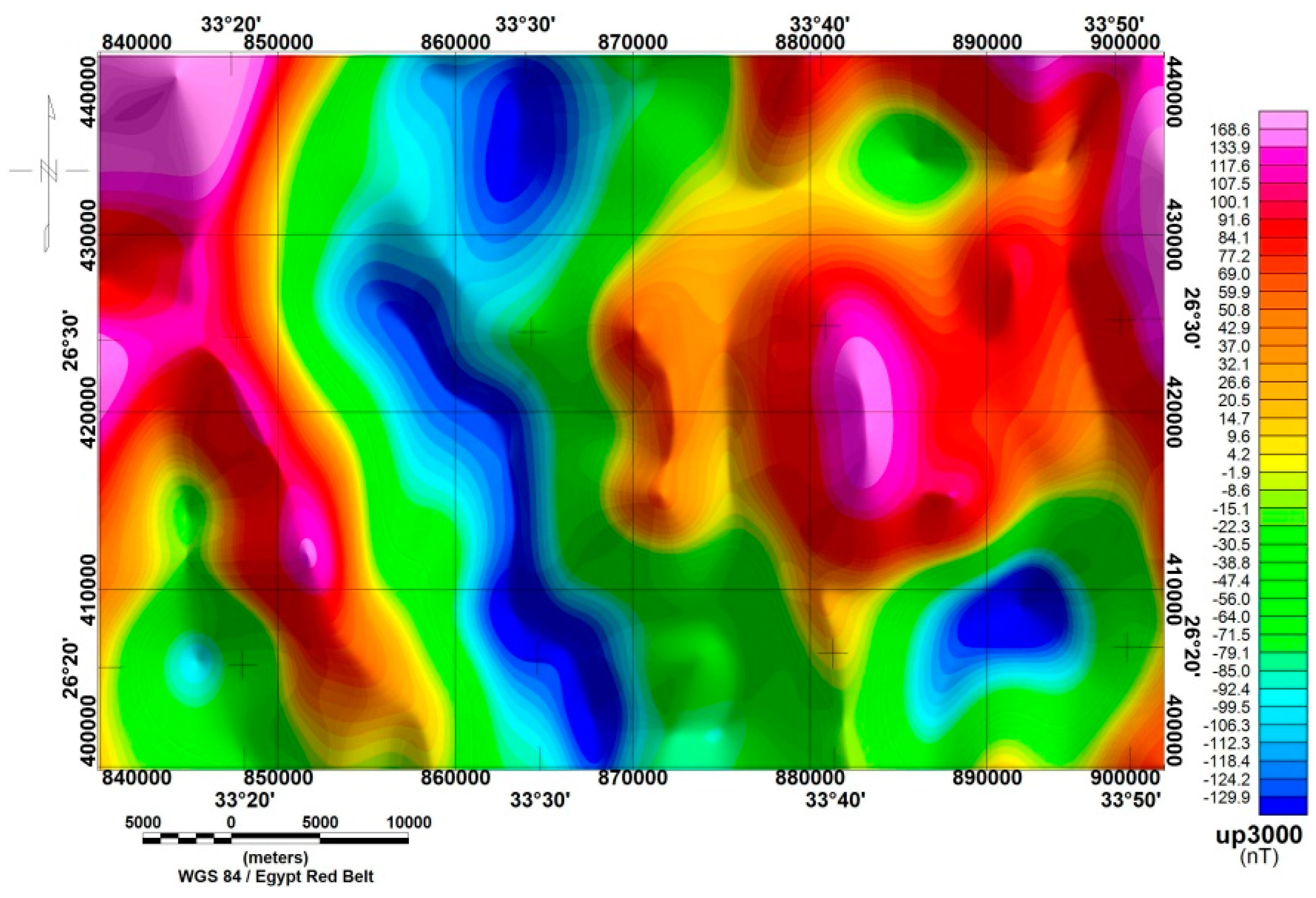
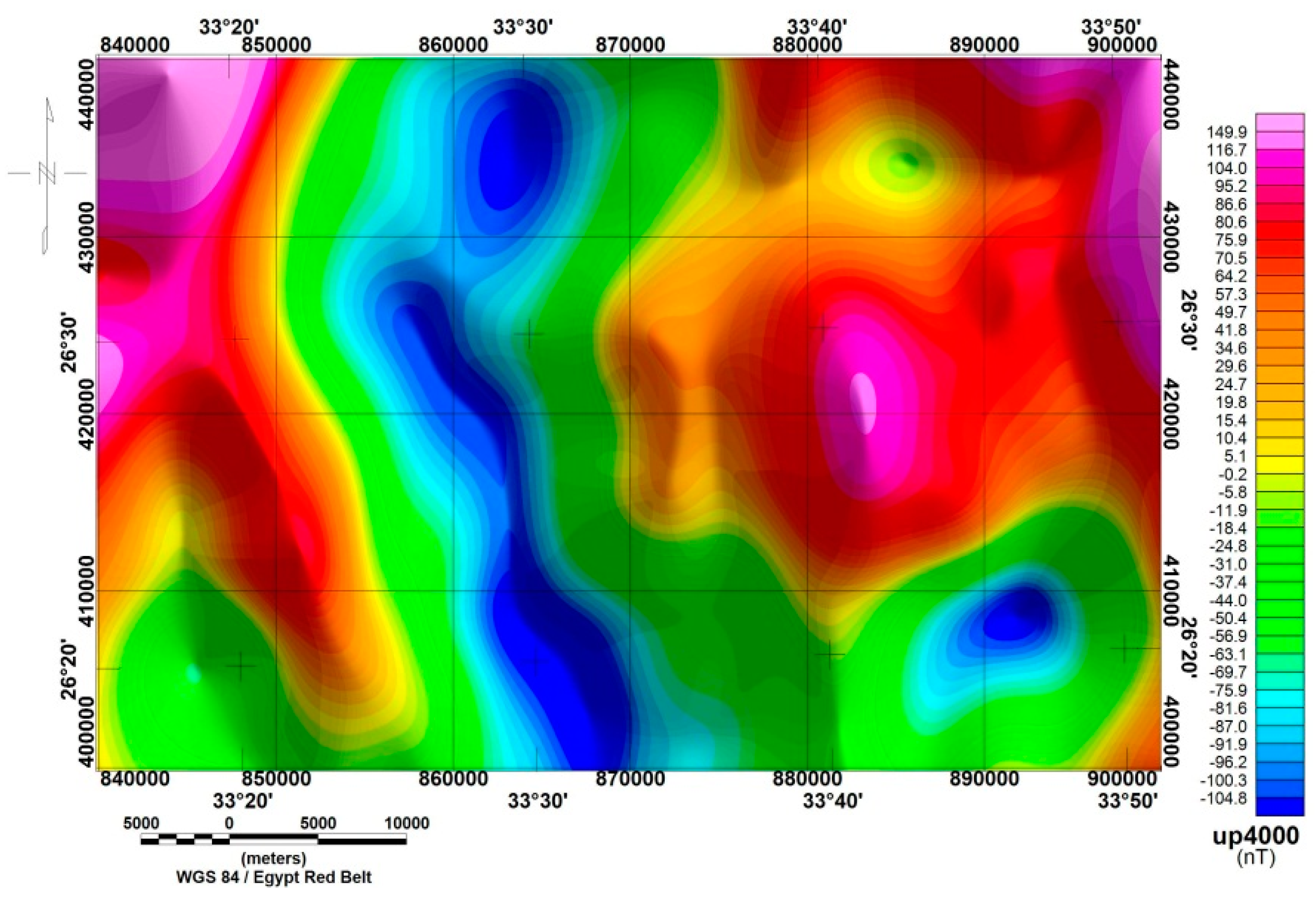
2.3. Upward Continuation

Upward continuation tends to highlight anomalies generated by deep sources, overshadowing anomalies caused by shallow sources [26,27,28]. It might be preferable to eliminate or alleviate localized disturbances caused by features with small lateral extents to better delineate large-scale structures, thereby offering a clearer depiction of the regional field [29,30,31]. The present study conducted the process of upward continuation for aeromagnetic anomalies on the RTP aeromagnetic map (Figure 4). This process utilized coefficients computed through a numerical evaluation of the Fourier transform in the frequency domain. The computation was carried out at four distinct levels by using different grid cell units (grid spacings) that correspond to average depths of 1.5, 2.0, 3.0, and 4.0 km, respectively. The Oasis Montaj™ software (version 7.1, [17]) was utilized for this computation. As a result, four maps (Figure 8, Figure 9, Figure 10 and Figure 11) were generated at the four levels mentioned above.

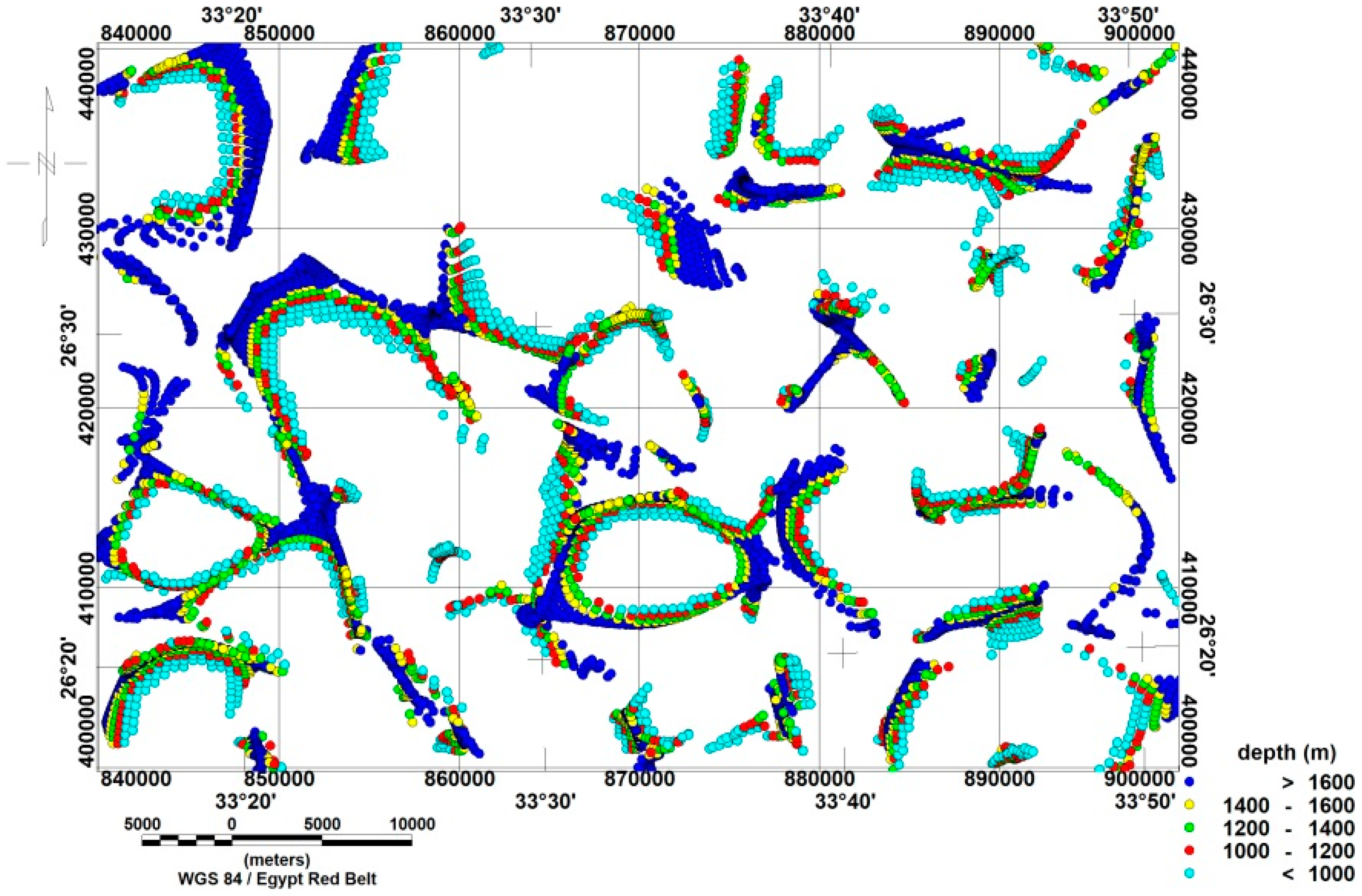
2.4. Euler Deconvolution

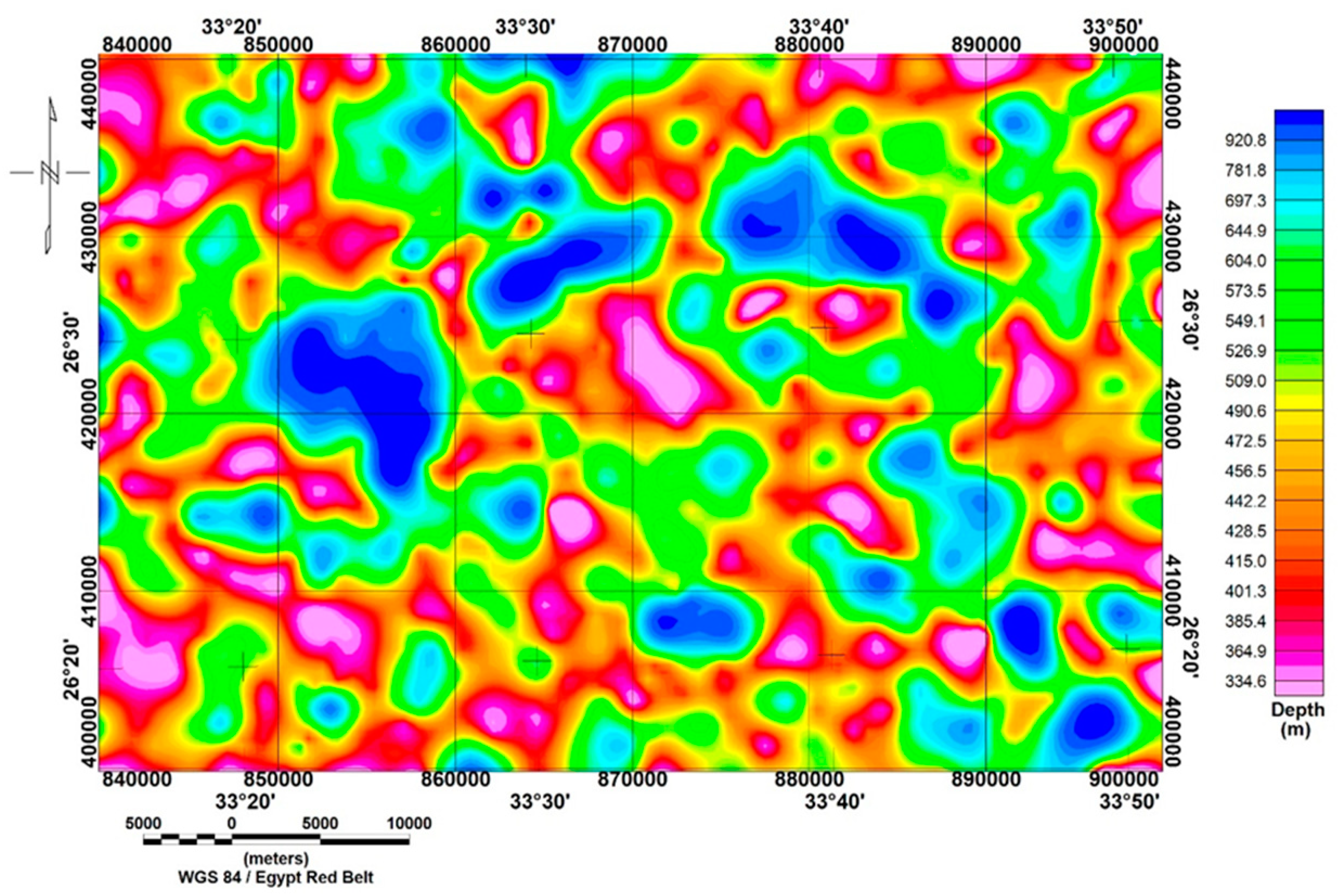
Euler deconvolution, employed as an interpretation method for potential field data, is firmly established as able to swiftly determine the source position and depth via deconvolution [32,33,34]. The technique involves using potential field data organized in a grid format. Euler’s homogeneity equation establishes a connection between the magnetic field and its derivative components, offering insights into the source’s location based on the degree of homogeneity, represented as N. This value can be interpreted as a particular indicator of structure. For example, a magnetic field linked to a contact possesses a structural index of N = 0, whereas for a fault, this is N = 0.5, and for a dyke/sill, this is N = 1. Nevertheless, in most practical scenarios, even when the structural index is tailored to a specific geometry, the solution may identify sources with a differing structural index. Euler’s equation is delineated by Ghosh et al. [35] and Golshadi et al. [36].

$$\left(x-x_0\right){\displaystyle \frac{\partial T}{\partial x}}+\left(y-y_0\right){\displaystyle \frac{\partial T}{\partial y}}+\left(z-z_0\right){\displaystyle \frac{\partial T}{\partial z}}=N\left(B-T\right),$$

(1)

where ${\displaystyle \frac{\partial T}{\partial x}},{\displaystyle \frac{\partial T}{\partial y}},$ and ${\displaystyle \frac{\partial T}{\partial z}}$ denote the initial derivatives of the field T along the three directions. The source’s position is denoted by coordinates (x₀, y₀ and z₀) and has a structural index N. The total field T is measured at (x, y, and z), with the total field possessing a regional value B.

The best source location is determined through the least squares inversion of the data within a selected window length. Typically, solutions are derived for various structural index values, and those exhibiting the most optimal clustering of the data are chosen. It was discovered that using smaller grid intervals resulted in noisy solutions [37,38,39]. The Euler solutions provided pertain to grid intervals of 0.5 km. In this study, the extended Euler deconvolution was conducted with a structural index (N) set to 0 to identify the magnetic contacts.

2.5. SPI Technique

In 1997, Thurston and Smith [18] pioneered Source Parameter Imaging (SPI), a methodology that emphasizes the augmentation of the expansive complex analytical signal. The primary objective of SPI is to ascertain the depths of magnetic sources. The connection between the source’s depth and the local wavenumber (W) of the magnetic field has been established in the context of SPI, as demonstrated by studies conducted by Fairhead et al. [40] Salem et al. [41] Al-Badani and Al-Wathaf [42], and Elhussein and Shokry [43] (2020). Determining the local wavenumber involves the computation of horizontal and vertical derivatives from the RTP grid. Al-Badani and Al-Wathaf [42] presented the formula for the local wavenumber function:

$$W\left(x,y\right)={\displaystyle \frac{\frac{{\partial }^{2}T}{\partial x\partial z}\frac{\partial T}{\partial x}+\frac{{\partial }^{2}T}{\partial y\partial z}\frac{\partial T}{\partial y}+\frac{{\partial }^{2}T}{{\partial }^{2}z}\frac{\partial T}{\partial z}}{{\left(\frac{\partial T}{\partial x}\right)}^2+{\left(\frac{\partial T}{\partial y}\right)}^2+{\left(\frac{\partial T}{\partial z}\right)}^2}},$$

(2)

In this framework, the term “W” is used to signify the local wave number, and ${\displaystyle \frac{\partial T}{\partial x}},{\displaystyle \frac{\partial T}{\partial y}},$ and ${\displaystyle \frac{\partial T}{\partial z}}$ denote the initial derivatives of the field T along the three directions. The formula, presented by Al-Badani Al-Wathaf [42], simplifies the computation of a magnetic source’s depth.

$$h_{x=0}={\displaystyle \frac{1}{W_{max}}},$$

(3)

In this scenario, $h_{x=0}$ denotes the calculated depth at the source’s boundary, while $W_{max}$ indicates the maximum value of the local wavenumber.

2.6. GPSO Technique

Eberhart and Kennedy [44] introduced particle swarm optimization in 1995. Currently, this method is utilized in various geophysical contexts, as documented in studies by Ourique et al. [45], Chau [46], Sen and Stoffa [47], Xiong and Zhang [48], Essa and Elhussein [49], Ekinci et al. [50], and Elhussein [43,51,52]. In this application, the stochastic approach is metaphorically compared to a group of birds seeking sustenance. Each model embodies the characteristics of birds, encompassing both a velocity vector and a position vector, which constitute the set of parameter values. The inversion process starts by randomly allocating models to the swarm, using potential ranges for different variables. The provided formulas are employed to update the velocity and position of the various models through a series of iterative steps.

$$x_i^{k+1}=x_i^k+S_i^{k+1},$$

(4)

$$S_i^{k+1}=\sigma S_i^k+\lambda f1\left(L_{best}-x_i^{k+1}\right)+\eta f2\left(P_{best}-x_i^{k+1}\right),$$

(5)

Equation (4) represents $x_i^k$ and $S_i^k$, which represent the position and speed of particle i during iteration k, respectively. The variables f1 and f2 represent two randomly generated numbers chosen from the interval [0,1]. The behavior of the particle is regulated by the cognitive coefficient (λ) and social coefficient (η), commonly assigned a value of 2 according to Equation (5) as indicated in studies by Singh and Biswas [53], Essa and Elhussein [49], and Pace et al. [54]. Furthermore, the inertial factor σ governs the model’s velocity, maintaining it at a value below one. $L_{best}$ indicates the optimal position reached by an individual model, whereas $P_{best}$ denotes the most favorable global position achieved by any model within the swarm. Subsequently, the optimal solutions $L_{best}$ and $P_{best}$ are saved in memory as the most favorable outcome. The velocity and position of the model experience iterative adjustments until reaching convergence, guided by the optimization of a designated objective function [55].

In this research, the application of GPSO was utilized to estimate various source parameters, including amplitude factor (A_f), depth (h), shape factor (S_f), and source location (x_o), across two RTP profiles.

3. Results and Discussion

The analysis of aeromagnetic data is a valuable method for structural mapping in areas such as Missiakat Al Jukh. It helps geologists and geophysicists to visualize subsurface structures, which play a key role in understanding the region’s geological history and guiding mineral exploration efforts. By combining aeromagnetic data with advanced processing techniques (such as RTP and filtering) and integrating them with other geophysical and geological information, the accuracy and reliability of interpretations are significantly improved.

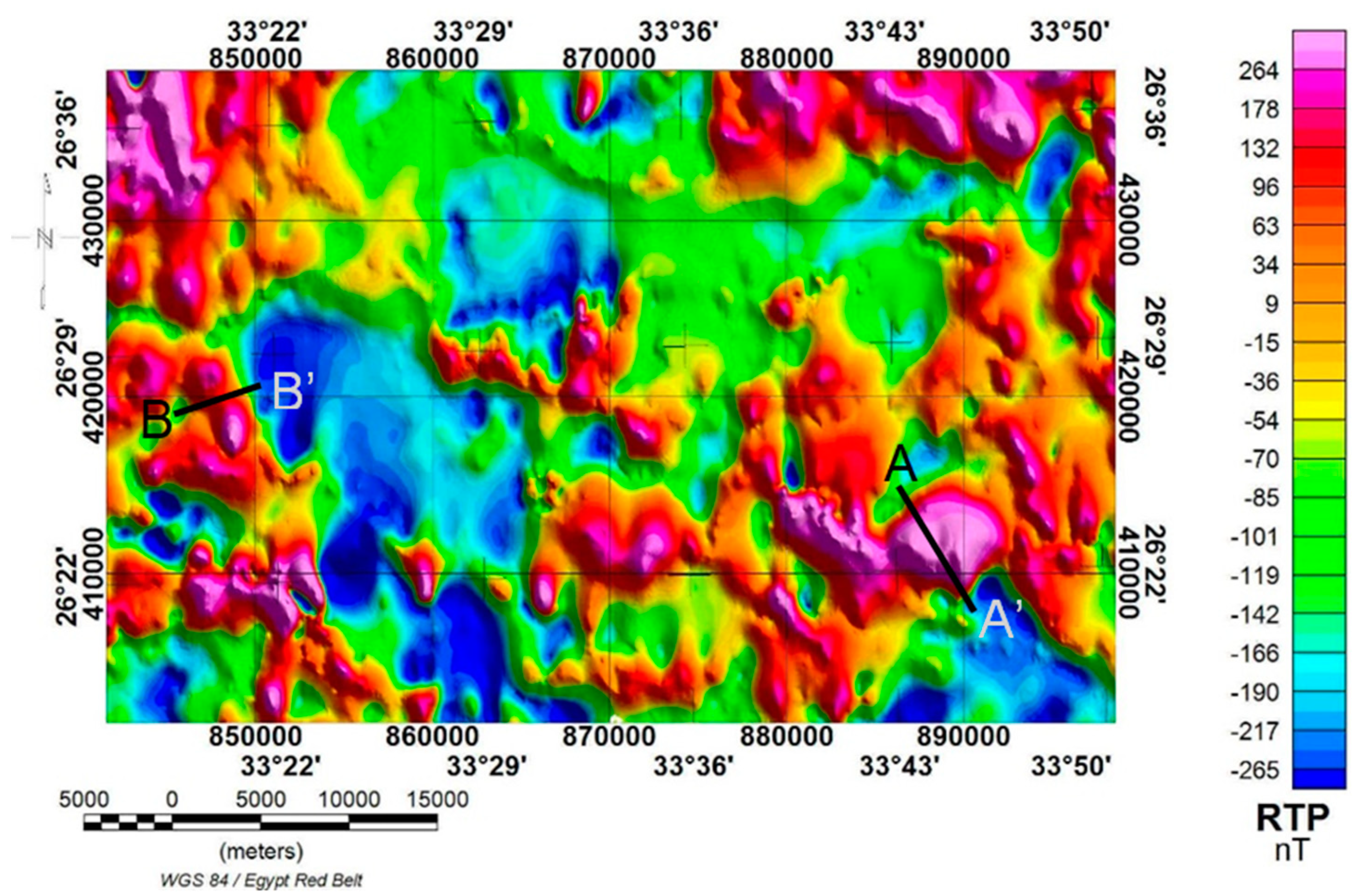
3.1. Aeromagnetic Maps (Observed, Regional, and Residual)

The original aeromagnetic map’s total intensity, depicted in Figure 3, exhibits three significant positive magnetic anomalies in the region’s southeastern, northeastern, and northwestern parts. Additionally, smaller anomalies are dispersed across the study site’s western, central, and eastern areas. These anomalies are linked to foundational rocks and distinguished by high amplitudes, primarily aligning in the northwest–southeast and east–west directions. Conversely, the study area’s central, northwestern, and southwestern parts predominantly exhibit negative magnetic anomalies. These anomalies exhibit low amplitudes and predominantly trend in northwest–southeast and east–west orientations, similar to the positive magnetic anomalies.

The RTP aeromagnetic intensity map (Figure 4) shows that the locations of previously identified magnetic anomalies have shifted northward compared to the original total aeromagnetic intensity map (Figure 3). This shift is attributed to the removal of the magnetic field inclination across the study area. The magnetic gradients of the RTP magnetic anomalies increase in intensity and steepness, resulting in an improved resolution and delineation of both the lithologic and structural features encountered.

A thorough analysis of the RTP aeromagnetic map (Figure 4) reveals multiple clusters of positive and negative magnetic anomalies characterized by different wavelengths, amplitudes, shapes, and sizes, corresponding to the types and depths of their source bodies.

Two magnetic anomalous zones were identified based on variations in their magnitudes and characteristics, including the wavelengths, amplitudes, areal distribution, and trend patterns of the anomalies. The initial anomalous region consists of a narrow belt of positive magnetic anomalies, exhibiting NNW to NW and E-W trends. This region covers the northeastern, northwestern, and southeastern sectors of the study zone and is linked with substantial occurrences of hornblende gabbro (ohgb), serpentinite (osm), xenolithic granodiorite (gt), hornblende gabbro and diorite (gbd), and hornblende monzodiorite (gb). The magnetic amplitudes of these anomalies gradually diminish towards the central, north–central, and south–central portions of the study area, potentially indicating their origin from deep-seated basic to ultrabasic sources.

The additional magnetic anomaly zone spans the study region’s north central, south central, and southeastern portions. This region exhibits numerous moderate to negative magnetic anomalies, predominantly aligned in the NNW and NE directions. These anomalies are primarily linked to the Upper Cretaceous Dokhan (kuda) and Tarif (kut) formations, as well as biotite alkali granite (gk), chlorite, quartz, and talc schist (mv), and epidote chlorite metabasic schist (mvb). Additionally, Quaternary Wadi sediments are present in the area.

Using Spectral Frequency Analysis, two primary average levels (interfaces) were calculated at depths of 0.6 and 1.3 km beneath the measuring level, revealing themselves on the spectrum curve for the near-surface and deep-seated magnetic components, respectively.

Figure 6 portrays a residual aeromagnetic component map, which distinctly illustrates numerous clusters of positive and negative magnetic anomalies. These anomalies demonstrate a higher resolution than those observed in the RTP aeromagnetic map. These anomalies exhibit almost semicircular and elongated shapes, characterized by their comparatively short wavelengths and high frequencies. Variations in frequency and amplitude can occur locally due to differences in composition or the depths from which sources originate. Major trends observed from the residual map indicate near-surface structures in the study region oriented in the NNW-SSE, ENE-WSW, N-S, NE-SW, and NW-SE directions.

The regional magnetic anomalies exhibit low frequencies and long wavelengths. Figure 7 presents a map of the deep-seated aeromagnetic components, depicting a variety of magnetic anomalies, both positive and negative in nature, which predominantly follow directions such as NNW-SSE, N-S, NW-SE, and NE-SW. Differences in compositions and/or relative depths to their sources could explain the local differences observed in the frequency and amplitude of these anomalies.

Upon careful analysis of the residual and regional aeromagnetic component maps depicted in Figure 6 and Figure 7, it appears that the concentration of magnetic anomalies of small sizes (clustered together), depicted in the RTP map (Figure 4), are also present on the residual and regional magnetic component maps. However, in the latter maps, they appear as singular, continuous, and broad aeromagnetic anomalies. These characteristics indicate that these small-scale anomalies may have a shared deep-seated origin and could thus be regarded as related. Some other magnetic anomalies have vanished from the regional aeromagnetic component map. Nevertheless, they remain observable on the RTP aeromagnetic and residual magnetic component maps (Figure 4 and Figure 6). These occurrences could indicate that these irregularities stem from magnetic sources near the surface, situated at shallow levels. The magnetic component map of the region (depicted in Figure 7) emphasizes the primary patterns influencing the underlying structures of the surveyed area. These structures primarily align with the NNW-SSE, NW-SE, and N-S directions.

A comparison between the aeromagnetic map at a 1.5 km elevation (Figure 8) and the regional anomaly map at an interface of 1.3 km (Figure 7) shows a notable resemblance. Despite this, both maps still display aeromagnetic anomalies with similar characteristics at this observation level, including wavelength, spatial distribution, and magnetic trends, with most residual bodies eliminated. Variations in the magnitude of magnetic anomalies in certain areas may result from differences in the algorithms utilized by the software for calculating the two processes. As a result, the shapes of the two maps closely match the ideal response; however, the amplitudes of these shapes vary by one or more units of the basic contour interval.

The upward continued map depicted at the 1.5 km level (Figure 8) demonstrates the presence of both high and low magnetic zones, which closely correspond to those observed on the regional airborne magnetic intensity component map (Figure 7), occurring nearly at the same locations. Certain aeromagnetic anomalies are demonstrated to be confined in extent to a maximum of 2.0 km (refer to Figure 9). Furthermore, certain aeromagnetic anomalies vanish from the upward continued maps when reaching the third and fourth levels at 3.0 and 4.0 km (see Figure 10 and Figure 11). However, they persist on the first and second upward continued maps (refer to Figure 8 and Figure 9). Based on this observation, it can be inferred that these magnetic anomalies might stem from depths exceeding 2.0 km but less than 3.0 km, indicating that they are shallow-rooted, near-surface anomalies. A careful examination of the four upward continued maps (Figure 8, Figure 9, Figure 10 and Figure 11) reveals that certain low (or high) magnetic zones diminish in a particular area while other high (or low) magnetic zones expand with higher observation levels. This observation may strongly suggest compositional variances in the underlying rocks as observation levels increase.

The aeromagnetic map extends up to 3 km (Figure 10), demonstrating the widespread impact of magnetic properties originating from deep-seated sources. It encompasses structural features and lithology variations within the basement and intra-basement throughout the surveyed region. The enduring effects stem from the initial RTP aeromagnetic map. As a result, the magnetic anomalies observed on this map may have deep origins and extend to the surface or relatively shallow depths.

The aeromagnetic maps extended to elevations of 3.0 and 4.0 km (refer to Figure 10 and Figure 11) illustrate that the study area can be partitioned into two magnetic features. The initial feature displays high magnetic properties and spans the northwestern and northeastern (uplifted blocks) sections. The subsequent feature exhibits low magnetic properties and encompasses the study area’s southeastern, central, and southwestern regions (subsided blocks). The subsided blocks are cut by various structural lineaments that trend in the ENE-WSW direction, which divides the uplifted blocks via the NNW-SSE structural lineaments. Numerous NE-SW trending structural lineaments dissect the eastern uplifted block, dividing it and the western uplifted block into multiple sub-blocks. Certain sub-blocks experience uplift (high trend) in the northern and southeastern regions. Conversely, another block undergoes subsidence (low trend) between these uplifted blocks, potentially forming a graben.

Examining upward continuation magnetic maps at levels of 1.5, 2, 3, and 4 km unveils the presence of seven magnetic highs, which underlie four low-magnetic belts, primarily oriented in a north–south direction. H1 lies along the western border of the map, with H2 to H7 extending easterly to the eastern border. The four low-magnetic belts are situated between the high-magnetic belts mentioned earlier. These patterns are consistent across all four maps depicting upward magnetic trends. As inferred from the four upward continued aeromagnetic maps (Figure 8, Figure 9, Figure 10 and Figure 11), the primary structural trends follow the NNW-SSE and ENE-WSW directions. Consequently, these two trends manifest as deep-seated features within the study area. The magnetic high trends indicate the presence of basic igneous rocks, whereas the magnetic low trends signify the presence of granitic igneous rocks.

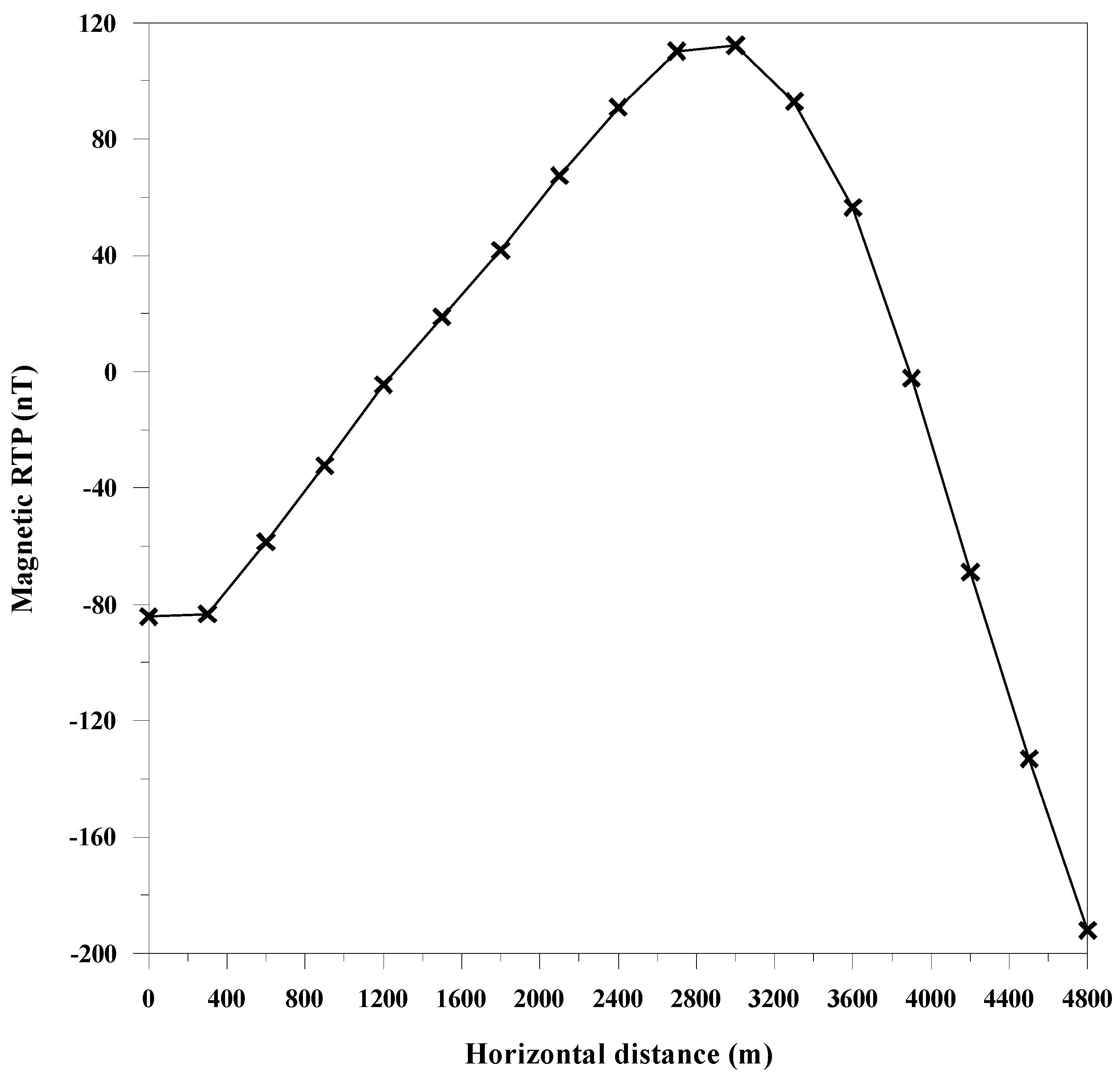
3.2. Subsurface Structure Estimation

Euler deconvolution was utilized to derive the magnetic contacts, as depicted in Figure 12. Additionally, the conventional clustering of depth solutions across the study area is presented. This map illustrates general trends in the principal structural indices, indicated by varying colors of circles and various clusterings, which signify different depths and trends. The Euler solutions depicted in Figure 12 offer insight when estimating the depth of magnetic sources. The Euler map (N = 0) exhibits clearly defined clusters of circles arranged in linear and curved patterns, revealing the potential locations of contacts that may arise from faulting. Moreover, the depth estimates obtained from the colored circles align perfectly with the regional magnetic map component (Figure 7).

The subsurface structures inferred from Euler deconvolution on the regional magnetic map (Figure 12), employing N = 0 (indicating contacts), reveal the presence of the deepest structural lineaments (exceeding 1600 m) and trends oriented in NNW-SSE, NNE-SSW, ENE-WSW, WNW-ESE, and E-W directions, which are notably prominent in the northern and central sectors of the study area. Most of the shallower structures (ranging from 0 to 1000 m) are located in the northwestern, southwestern, and southeastern regions, as well as certain areas within the central zone of the study. These structures display orientations in the NNW-SSE, N-S, and ENE-WSW directions, with their contacts determined to be structurally influenced. Moreover, the depth estimates inferred from the colored circles correspond seamlessly with the regional magnetic map component (Figure 7).

Utilizing the SPI technique shows that magnetic sources at the research location vary in depth, ranging from 283 to 1600 m, and exhibit an average depth of around 529.3 m (Figure 13).

Using GPSO technique across two RTP profiles (Figure 14), the estimated parameters include A_f = 9564.53 nT, h = 105.37 m, S_f = 0.94, and x_o = 3618.29 m for profile 1 (Figure 15), while, in the case of profile 2 (Figure 16), the estimated parameters are A_f = 7391.96 nT, h = 147.61 m, S_f = 1.07, and x_o = 2551.38 m. The estimated results from different techniques matched well.

Given that the area under examination primarily comprises igneous, metamorphic, and sedimentary rocks, which exhibit a wide range of compositions (including both acidic and basic constituents), these rocks have been influenced by diverse regional and local geological structures of varying types, magnitudes, trends, and locations. Because the prevailing Precambrian basement rocks in the area of interest typically exhibit faulting as a prominent structural feature, it is anticipated that faulting is more developed than other structural elements. This is why we chose not to use N = 0.5 for Euler deconvolution.

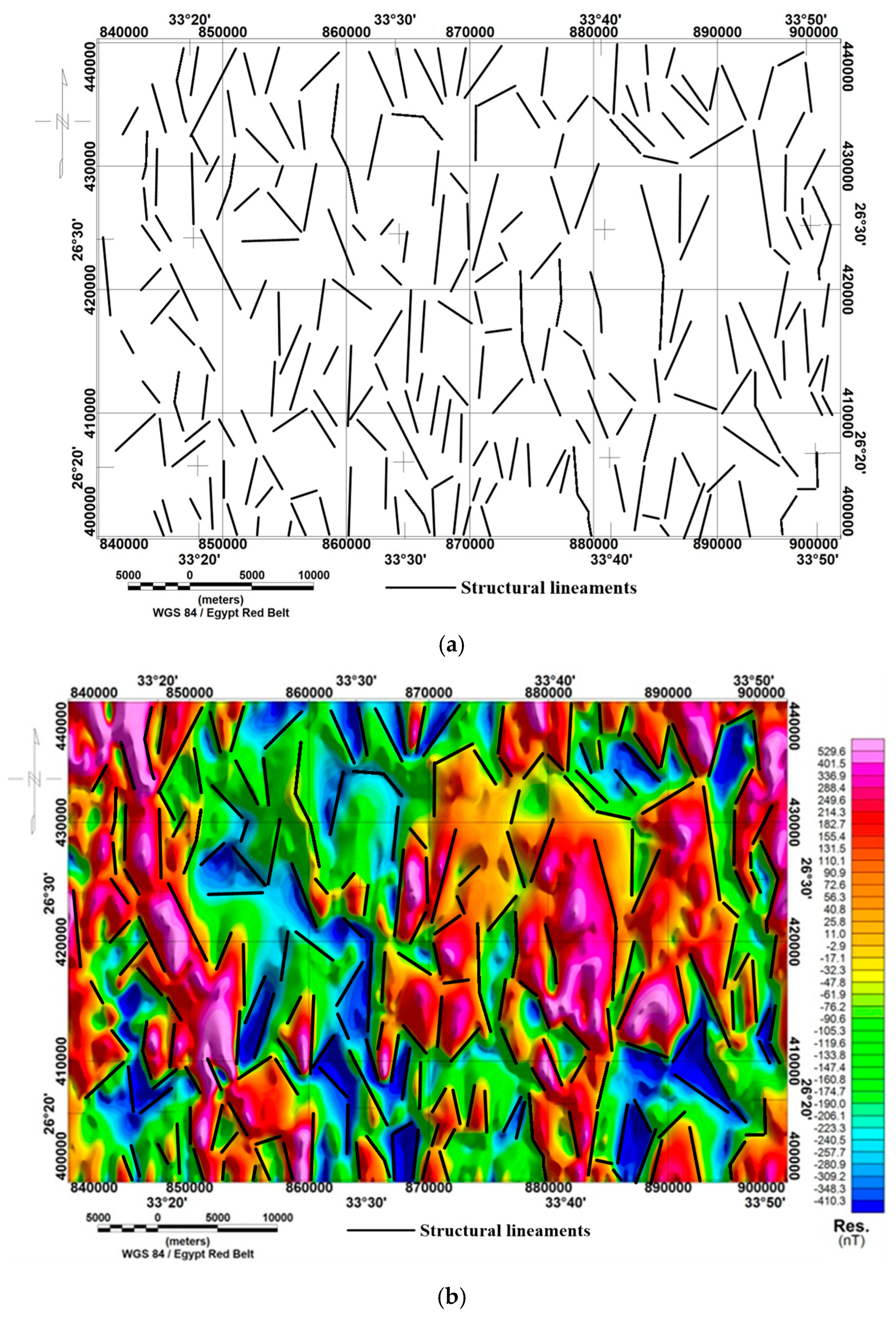
3.3. Structural Lineament Maps

The Rose Diagram Technique is a straightforward and widely used method for depicting two-dimensional patterns. It constructs a frequency plot that displays the percentage of trends in different directional ranges. In this technique, lineation trends are categorized into 10-degree intervals, with their lengths or counts within each class totaled and expressed as a percentage of all trends’ overall lengths or counts. The frequency distribution is then charted with respect to direction, both clockwise and counterclockwise from the north.

In this study, we interpreted the aeromagnetic survey data by creating two structural lineaments maps (Figure 17a,b and Figure 18a,b), one for shallow-seated features and the other for deep-seated features. These lineaments were interpreted based on qualitative analysis (observing the magnetic anomalies) and further refined by integrating this analysis with edge detection filters, such as Euler deconvolution. Additionally, we produced Rose diagrams of the main lineament features (Figure 19a,b). These maps illustrate the overall structural framework of the study area and highlight its primary structural features.

Referring to the residual (shallow-seated) magnetic structural lineaments map (Figure 17a,b) and the Rose diagram of its lineament features, it is evident that the structural features cutting through the basement rocks are more pronounced than those at the deeper interface. These elements become more densely packed and concentrated as they ascend. However, the structural features depicted in this map (Figure 17a,b) and its Rose diagram differ significantly from those shown in the regional magnetic structural lineaments map (Figure 18a,b), exhibiting a higher level of complexity in the residual map. Two major structural trends are observed: (a) NNW-SSE, and (b) E-W or ENE-WSW. The intersection of these trends creates horsts, grabens, and fault patterns resembling steps, which collectively determine the structural layout of the underlying basement rocks.

The regional (deep-seated) magnetic structural lineaments map (Figure 18a,b) primarily reflects substantial changes in composition within the concealed crystalline basement complex (intra-basement magnetic influence), along with prominent structural relief features at a larger scale (supra-basement magnetic influence). In contrast, the residual (near-surface) magnetic structural lineaments map (Figure 17a,b) is primarily shaped by the magnetic basement complex’s intricate, small-scale structural characteristics.

The study area is characterized by numerous faults and lineaments that intersect with wadis, drainage lines, and rock contacts. These faults predominantly trend in the NNW-SSE, ENE-WSW, N-S, and E-W directions.

The magnetic signatures depicted in the regional and residual magnetic structural lineament maps (Figure 17a,b and Figure 18a,b) and the Rose diagrams of the main lineament features (Figure 19a,b) reveal alternating high- and low-magnetic zones. The low-magnetic zones likely correspond to structural lows, such as down-thrown blocks or grabens, while the high-magnetic zones that separate them likely correspond to structural highs, such as up-faulted blocks or horsts. The precise boundaries between these zones, which exhibit significantly different magnetic characteristics, may suggest the presence of significant basement faults and/or contacts. Furthermore, the abrupt changes in magnetic anomaly trends are associated with systematic structural lineaments indicative of faults. These magnetic structural lineaments, which extensively dissect the study area, are illustrated on the two structural lineament maps (Figure 17a,b and Figure 18a,b).

4. Conclusions

The structural framework of the study area was effectively mapped by integrating various interpretation techniques and applying them to aeromagnetic survey data. Through the analysis of the regional power spectrum of the aeromagnetic data, two primary interfaces were identified at depths of 0.6 and 1.3 km below the surface. Using Gaussian filtering, regional magnetic sources were detected at 1.3 km depth, while residual magnetic sources were located at 0.6 km. The upward continuation technique, applied at four different levels (1.5, 2.0, 3.0, and 4.0 km), revealed high- and low-magnetic zones, successfully eliminating most residual bodies. At the 3.0 and 4.0 km levels, significant magnetic anomalies (masses) were delineated and isolated by major structural lineaments oriented in NNW-SSE, ENE-WSW, N-S, and E-W directions. The area is influenced by three primary structural trends: NNW, N-S, and ENE. The Euler Deconvolution technique was applied to estimate the depths of the causative magnetic bodies, aiding in the identification of subsurface contacts.

This study makes a significant contribution to sustainable resource exploration by enhancing the understanding of subsurface structures and potential mineral deposits. By integrating aeromagnetic data with geological information, tectonic maps were produced at depths of 0.6 km and 1.3 km, showing a gradual increase in the density and concentration of structural lineaments from deeper to shallower levels. These findings provide valuable insights into the structural framework, enabling more precise exploration and reducing unnecessary drilling, which in turn lowers the environmental impact of resource extraction. Additionally, the detailed mapping of both deeper regional structures and shallower residual structures provides crucial data for the development of sustainable exploration strategies, optimizing resource use, and promoting environmental responsibility. This research supports more efficient exploration practices by identifying structural patterns that influence resource distribution, aligning with global sustainability goals and fostering the responsible management of natural resources.

References

1. Hamimi, Z.; Abd El-Wahed, M.; Gahlan, H.; Kamh, S. Tectonics of the Eastern Desert of Egypt: Key to understanding the neoproterozoic evolution of the Arabian–Nubian Shield (East African Orogen). In The Geology of the Arab World—An Overview; Springer: Berlin/Heidelberg, Germany, 2019; pp. 1–81. [Google Scholar]
2. Hamimi, Z.; Abd El-Wahed, M.A. Suture (s) and major shear zones in the Neoproterozoic basement of Egypt. In The Geology of Egypt; Springer: Berlin/Heidelberg, Germany, 2020; pp. 153–189. [Google Scholar]
3. EGSMA. Geologic Map of Al-Qusayr Quadrangle; EGSMA: Cairo, Egypt, 1992. [Google Scholar]
4. Nabawy, B.S.; Barakat, M.K. Formation evaluation using conventional and special core analyses: Belayim Formation as a case study, Gulf of Suez, Egypt. Arab. J. Geosci. 2017, 10, 1–23. [Google Scholar] [CrossRef]
5. El-Gendy, N.; Barakat, M.; Abdallah, H. Reservoir assessment of the Nubian sandstone reservoir in South Central Gulf of Suez, Egypt. J. Afr. Earth Sci. 2017, 129, 596–609. [Google Scholar] [CrossRef]
6. Abdelwahab, F.; El Gendy, N.; Barakat, M.K.; Mohamed, M.; El-Tohamy, A.; El Terb, R.; El Feky, M. Radionuclide Content and Radiation Dose Rates of Uraniferous and Mineralized Granites at GV Occurrence in Gabal Gattar, Northeastern Desert, Egypt. J. Phys. Conf. Ser. 2022, 2305, 012006. [Google Scholar] [CrossRef]
7. Azab, A.; Nabawy, B.S.; Mogren, S.; Saqr, K.; Ibrahim, E.; Qadri, S.T.; Barakat, M.K. Structural Assessment and Petrophysical Evaluation of the pre-Cenomanian Nubian Sandstone in the October Oil Field, Central Gulf of Suez, Egypt. J. Afr. Earth Sci. 2024, 218, 105351. [Google Scholar] [CrossRef]
8. Reford, M.; Sumner, J. Aeromagnetics. Geophysics 1964, 29, 482–516. [Google Scholar] [CrossRef]
9. Oruç, B.; Selim, H. Interpretation of magnetic data in the Sinop area of Mid Black Sea, Turkey, using tilt derivative, Euler deconvolution, and discrete wavelet transform. J. Appl. Geophys. 2011, 74, 194–204. [Google Scholar] [CrossRef]
10. Deng, Y.; Chen, Y.; Wang, P.; Essa, K.S.; Xu, T.; Liang, X.; Badal, J. Magmatic underplating beneath the Emeishan large igneous province (South China) revealed by the COMGRA-ELIP experiment. Tectonophysics 2016, 672, 16–23. [Google Scholar] [CrossRef]
11. Minelli, L.; Speranza, F.; Nicolosi, I.; D’Ajello Caracciolo, F.; Carluccio, R.; Chiappini, S.; Messina, A.; Chiappini, M. Aeromagnetic investigation of the central Apennine Seismogenic Zone (Italy): From basins to faults. Tectonics 2018, 37, 1435–1453. [Google Scholar] [CrossRef]
12. Ekwok, S.E.; Achadu, O.-I.M.; Akpan, A.E.; Eldosouky, A.M.; Ufuafuonye, C.H.; Abdelrahman, K.; Gómez-Ortiz, D. Depth estimation of sedimentary sections and basement rocks in the Bornu Basin, Northeast Nigeria using high-resolution airborne magnetic data. Minerals 2022, 12, 285. [Google Scholar] [CrossRef]
13. Zhu, X.; Wang, L.; Zhou, X. Structural features of the Jiangshao Fault Zone inferred from aeromagnetic data for South China and the East China Sea. Tectonophysics 2022, 826, 229252. [Google Scholar] [CrossRef]
14. Aero-Service. Final Operational Report of Airborne Magnetic/Radiation Survey in the Eastern Desert, Egypt; For the Egyptian General Petroleum Corporation (EGPC) and the Egyptian Geological Survey and Mining Authority (EGSMA); Aero-Service: Houston, TX, USA, 1984. [Google Scholar]
15. Wijns, C.; Perez, C.; Kowalczyk, P. Theta map: Edge detection in magnetic data. Geophysics 2005, 70, L39–L43. [Google Scholar] [CrossRef]
16. Li, X. Magnetic reduction-to-the-pole at low latitudes: Observations and considerations. Lead. Edge 2008, 27, 990–1002. [Google Scholar] [CrossRef]
17. Oasis Montaj Program v7.1. Geosoft Mapping and Processing System, version 7.1; Geosoft Inc.: Toronto, ON, Canada, 2010.
18. Baranov, V.; Naudy, H. Numerical calculation of the formula of reduction to the magnetic pole. Geophysics 1964, 29, 67–79. [Google Scholar] [CrossRef]
19. Baranov, V. Potential fields and their transformations in applied geophysics. J. Geod. 1975, 50, 1. [Google Scholar]
20. Bhattacharyya, B. Two-dimensional harmonic analysis as a tool for magnetic interpretation. Geophysics 1965, 30, 829–857. [Google Scholar] [CrossRef]
21. Bhattacharyya, B. Recursion filters for digital processing of potential field data. Geophysics 1976, 41, 712–726. [Google Scholar] [CrossRef]
22. Curtis, C.; Jain, S. Determination of volcanic thickness and underlying structures from aeromagnetic maps in the Silet area of Algeria. Geophysics 1975, 40, 79–90. [Google Scholar] [CrossRef]
23. Florio, G.; Fedi, M.; Rapolla, A. Interpretation of regional aeromagnetic data by the scaling function method: The case of Southern Apennines (Italy). Geophys. Prospect. 2009, 57, 479–489. [Google Scholar] [CrossRef]
24. Rerbal, L.; Bouyahiaoui, B.; Marok, A.; Abtout, A.; Boukerbout, H.; Bensefia, K.E. Use of aeromagnetic data for structural mapping of the Tlemcen Mountains (northwestern Algeria). Turk. J. Earth Sci. 2023, 32, 666–684. [Google Scholar] [CrossRef]
25. Telford, W.M.; Geldart, L.P.; Sheriff, R.E. Applied Geophysics; Cambridge University Press: Cambridge, UK, 1990. [Google Scholar]
26. Kaufman, A.A. Geophysical Field Theory and Method, Part A: Gravitational, Electric, and Magnetic Fields; Academic Press: Cambridge, MA, USA, 1992. [Google Scholar]
27. Blakely, R.J. Potential Theory in Gravity and Magnetic Applications; Cambridge University Press: Cambridge, UK, 1996. [Google Scholar]
28. Campbell, W.H. Introduction to Geomagnetic Fields; Cambridge University Press: Cambridge, UK, 2003. [Google Scholar]
29. Tsay, L.J. The use of Fourier series method in upward continuation with new improvements. Geophys. Prospect. 1975, 23, 28–41. [Google Scholar] [CrossRef]
30. Fedi, M.; Rapolla, A.; Russo, G. Upward continuation of scattered potential field data. Geophysics 1999, 64, 443–451. [Google Scholar] [CrossRef]
31. Wang, B. 2D and 3D potential-field upward continuation using splines. Geophys. Prospect. 2006, 54, 199–209. [Google Scholar] [CrossRef]
32. Reid, A.B. Euler deconvolution: Past, present and future-A review. Expanded Abstracts. In Proceedings of the 65th SEG Meeting, Houston, TX, USA, 8–13 October 1995; pp. 272–273. [Google Scholar]
33. Reid, A.B.; Allsop, J.; Granser, H.; Millett, A.T.; Somerton, I. Magnetic interpretation in three dimensions using Euler deconvolution. Geophysics 1990, 55, 80–91. [Google Scholar] [CrossRef]
34. Pei, J.; Li, H.; Wang, H.; Si, J.; Sun, Z.; Zhou, Z. Magnetic properties of the Wenchuan earthquake fault scientific drilling project Hole-1 (WFSD-1), Sichuan Province, China. Earth Planets Space 2014, 66, 23. [Google Scholar] [CrossRef]
35. Ghosh, G.; Khanna, A.; Singh, S. Application of euler deconvolution of gravity and magnetic data for basement depth estimation in Mizoram area. In Proceedings of the 5th EAGE St. Petersburg International Conference and Exhibition on Geosciences-Making the Most of the Earths Resources, Saint Petersburg, Russia, 2–5 April 2012; p. cp-283-00125. [Google Scholar]
36. Golshadi, Z.; Ramezanali, A.K.; Kafaei, K. Interpretation of magnetic data in the Chenar-e Olya area of Asadabad, Hamedan, Iran, using analytic signal, Euler deconvolution, horizontal gradient and tilt derivative methods. Boll. Geofis. Teor. Appl. 2016, 57, 329–342. [Google Scholar]
37. Gerovska, D.; Araúzo-Bravo, M.J. Automatic interpretation of magnetic data based on Euler deconvolution with unprescribed structural index. Comput. Geosci. 2003, 29, 949–960. [Google Scholar] [CrossRef]
38. Dewangan, P.; Ramprasad, T.; Ramana, M.V.; Desa, M.; Shailaja, B. Automatic interpretation of magnetic data using Euler deconvolution with nonlinear background. Pure Appl. Geophys. 2007, 164, 2359–2372. [Google Scholar] [CrossRef]
39. Melo, F.F.; Barbosa, V.C. Correct structural index in Euler deconvolution via base-level estimates. Geophysics 2018, 83, J87–J98. [Google Scholar] [CrossRef]
40. Fairhead, J.; Williams, S.; Flanagan, G. Testing magnetic local wavenumber depth estimation methods using a complex 3D test model. In SEG Technical Program Expanded Abstracts 2004; Society of Exploration Geophysicists: Sydney, NSW, Australia, 2004; pp. 742–745. [Google Scholar]
41. Salem, A.; Green, C.; Cheyney, S.; Fairhead, J.D.; Aboud, E.; Campbell, S. Mapping the depth to magnetic basement using inversion of pseudogravity: Application to the Bishop model and the Stord Basin, northern North Sea. Interpretation 2014, 2, T69–T78. [Google Scholar] [CrossRef]
42. Al-Badani, M.A.; Al-Wathaf, Y.M. Using the aeromagnetic data for mapping the basement depth and contact locations, at southern part of Tihamah region, western Yemen. Egypt. J. Pet. 2018, 27, 485–495. [Google Scholar] [CrossRef]
43. Elhussein, M.; Shokry, M. Use of the airborne magnetic data for edge basalt detection in Qaret Had El Bahr area, Northeastern Bahariya Oasis, Egypt. Bull. Eng. Geol. Environ. 2020, 79, 4483–4499. [Google Scholar] [CrossRef]
44. Eberhart, R.; Kennedy, J. A new optimizer using particle swarm theory. In Proceedings of the MHS’95. Sixth International Symposium on Micro Machine and Human Science, Nagoya, Japan, 4–6 October 1995; pp. 39–43. [Google Scholar]
45. Ourique, C.O.; Biscaia, E.C., Jr.; Pinto, J.C. The use of particle swarm optimization for dynamical analysis in chemical processes. Comput. Chem. Eng. 2002, 26, 1783–1793. [Google Scholar] [CrossRef]
46. Chau, W. Application of a particle swarm optimization algorithm to hydrological problems. In Water Resources Research Progress; Nova Science Publishers: New York, NY, USA, 2008; pp. 3–12. [Google Scholar]
47. Sen, M.K.; Stoffa, P.L. Global Optimization Methods in Geophysical Inversion; Cambridge University Press: Cambridge, UK, 2013. [Google Scholar]
48. Xiong, J.; Zhang, T. Multiobjective particle swarm inversion algorithm for two-dimensional magnetic data. Appl. Geophys. 2015, 12, 127–136. [Google Scholar] [CrossRef]
49. Essa, K.S.; Elhussein, M. Gravity data interpretation using different new algorithms: A comparative study. In Gravity-Geoscience Applications, Industrial Technology and Quantum Aspect; IntechOpen: London, UK, 2018. [Google Scholar]
50. Ekinci, Y.L.; Balkaya, Ç.; Göktürkler, G. Parameter estimations from gravity and magnetic anomalies due to deep-seated faults: Differential evolution versus particle swarm optimization. Turk. J. Earth Sci. 2019, 28, 860–881. [Google Scholar]
51. Elhussein, M. New inversion approach for interpreting gravity data caused by dipping faults. Earth Space Sci. 2021, 8, e2020EA001075. [Google Scholar] [CrossRef]
52. Elhussein, M. A novel approach to self-potential data interpretation in support of mineral resource development. Nat. Resour. Res. 2020, 30, 97–127. [Google Scholar] [CrossRef]
53. Singh, A.; Biswas, A. Application of global particle swarm optimization for inversion of residual gravity anomalies over geological bodies with idealized geometries. Nat. Resour. Res. 2016, 25, 297–314. [Google Scholar] [CrossRef]
54. Pace, F.; Santilano, A.; Godio, A. A review of geophysical modeling based on particle swarm optimization. Surv. Geophys. 2021, 42, 505–549. [Google Scholar] [CrossRef]
55. Venter, G.; Sobieszczanski-Sobieski, J. Multidisciplinary optimization of a transport aircraft wing using particle swarm optimization. Struct. Multidiscip. Optim. 2004, 26, 121–131. [Google Scholar] [CrossRef]
Figure 1. Location map of the Missiakat AL-Jukh area, Central Eastern Desert, Egypt.
Sustainability 16 08764 g001
Figure 2. Geologic map of Missiakat AL-Jukh area, Central Eastern Desert, Egypt, (EGSMA [3]).
Sustainability 16 08764 g002
Figure 3. Airborne magnetic intensity map.
Sustainability 16 08764 g003
Figure 4. Airborne RTP magnetic intensity map.
Sustainability 16 08764 g004
Figure 5. Interface determination using the local power spectrum of the airborne magnetic intensity data.
Sustainability 16 08764 g005
Figure 6. Residual airborne magnetic intensity component map, at an interface of 0.6 km.
Sustainability 16 08764 g006
Figure 7. Regional airborne magnetic intensity component map, at an interface of 1.3 km.
Sustainability 16 08764 g007
Figure 8. Upward continuation of the airborne magnetic intensity map at 1.5 km level.
Sustainability 16 08764 g008
Figure 9. Upward continuation of the airborne magnetic intensity map at 2 km level.
Sustainability 16 08764 g009
Figure 10. Upward continuation of the airborne magnetic intensity map at 3 km level.
Sustainability 16 08764 g010
Figure 11. Upward continuation of the airborne magnetic intensity map at 4 km level.
Sustainability 16 08764 g011
Figure 12. Euler depth of the airborne magnetic intensity map.
Sustainability 16 08764 g012
Figure 13. Depth mapping of the Missiakat AL-Jukh area, Central Eastern Desert, Egypt, determined through the implementation of the SPI technique.
Sustainability 16 08764 g013
Figure 14. Map showing the position of the two RTP magnetic profiles for the application of the GPSO technique across the study area.
Sustainability 16 08764 g014
Figure 15. Illustration of the reduced-to-pole magnetic anomaly profile (A–A’) obtained in the Missiakat AL-Jukh area within Central Eastern Desert, Egypt.
Sustainability 16 08764 g015
Figure 16. Illustration of the reduced-to-pole magnetic anomaly profile (B–B’) obtained in the Missiakat AL-Jukh area within Central Eastern Desert, Egypt.
Sustainability 16 08764 g016
Figure 17. (a). Shallow-seated structural lineaments map of the study area, deduced from residual magnetic data. (b). Shallow-seated structural lineaments overlaid on the residual magnetic map of the study area.
Sustainability 16 08764 g017
Figure 18. (a) Deep-seated structural lineaments map of the study area, deduced from regional magnetic data. (b) Deep-seated structural lineaments overlaid on the regional magnetic map of the study area.
Sustainability 16 08764 g018
Figure 19. (a). Rose diagram for shallow-seated structure of the study area. (b) Rose diagrams for deep-seated structure of the study area.
Sustainability 16 08764 g019
Disclaimer/Publisher’s Note: The statements, opinions and data contained in all publications are solely those of the individual author(s) and contributor(s) and not of MDPI and/or the editor(s). MDPI and/or the editor(s) disclaim responsibility for any injury to people or property resulting from any ideas, methods, instructions or products referred to in the content.