Abstract
The present study aims to address the knowledge gaps in dynamic power cable designs suitable for large floating wind turbines and to develop three baseline power cable designs. The study includes a detailed database of structural and mechanical properties for three reference cable models rated at 33 kV, 66 kV, and 132 kV to be readily used in global dynamic response simulations. Structural properties are obtained from finite element method (FEM) models of respective cable cross-sections built in UFLEX v2.8.9—a non-linear stress analysis program. Extensive mesh sensitivity studies are performed to ensure the accuracy of the predicted structural properties. The cable’s structural design is investigated using global response simulations of an OC3 5MW reference wind turbine coupled with the dynamic power cable in a lazy wave configuration. The feasibility of the present reference cable in floating offshore wind applications is assessed through a simplified analysis of cable fatigue life and structural integrity analysis of the cable in extreme environmental conditions. The analysis results suggest that the dynamic power cable does not significantly affect the response characteristics of the floating wind turbine in the analyzed lazy wave configuration. Furthermore, a simplified fatigue analysis demonstrates that the proposed cable design can sustain representative environmental loading scenarios and shows favorable dynamic performance in a lazy wave configuration.
1. Introduction
The global energy sector is witnessing a significant shift towards renewable energy sources, with wind energy emerging as a leading option. Offshore wind energy, in particular, is undergoing rapid development and upscaling. In the early 1980s, wind turbines had relatively small power ratings, reaching ~50 kW with rotor diameters approaching 15 m. Up to this day, the turbine size has grown significantly, reaching 18 MW with 260 m rotor diameter [1]. The upscaling aims to reduce the Levelized Cost of Energy (LCOE), rendering offshore wind energy more competitive with traditional energy sources. By investing in larger offshore wind farms, there is potential to harness wind power more effectively and sustainably. An estimated 80% of the world’s offshore wind resource potential lies in waters deeper than 60 m, where traditional bottom-fixed wind turbines are not feasible [2]. An outcome is the discernible shift towards the advancement of floating wind turbines for harnessing deep-sea wind resources. Floating offshore wind turbines (FOWTs) and substations necessitate the use of dynamic power cables specifically designed to withstand the complex motions induced by environmental forces such as waves, wind, and currents [3]. The optimization of inter-array cable configurations emerges as one of the key areas for LCOE reduction in offshore wind projects, where cable-related costs constitute approximately 20–30% of the total capital expenditure, as highlighted by Cozzi et al. [4]. In the initial stages of project development, the implementation of accurate and realistic reference power cables is imperative. Advanced numerical models are essential for predicting the fatigue life of the cables and optimizing the layout of the inter-array cable system. As the industry moves towards developing larger turbines with capacities exceeding 20 MW, there is a concurrent need to establish reference designs for suitable dynamic power cables. Such reference designs must accommodate the increased capacity demands and operational challenges associated with large-scale floating wind turbines.
The construction of a dynamic power cable typically consists of multiple material types arranged in several layers combined in a cylindrical or helical configuration [5]. Hence, the power cable can be considered as a multilayer, non-bonded composite flexible structure. Such structures exhibit non-linear mechanical behavior resulting from friction and sliding between components. Due to low bending and torsional stiffness properties, dynamic power cables are flexible in bending and torsional degrees of freedom while having a large axial stiffness. Experimental studies by Maioli [6] indicate that cable construction, e.g., layer arrangement and materials, have a profound influence on the resultant bending stiffness of the cable.
The theoretical foundations of mechanics of helically wound structures were established by Love [7], who derived the theory of thin rods. Love’s theory provided equations describing the equilibrium state of helical rods under external forces and moments. This theory was further expanded by Phillips et al. [8,9], who adapted Love’s framework to model twisted wire ropes analytically. The internal friction effects during bending were investigated by Lutchansky [10], and Vinogradov and Atatekin [11] explored the hysteretic behavior of bending stiffness. A significant advancement was the orthotropic model developed by Hobbs and Raoof [12], where each helical layer is simplified as an orthotropic cylinder. This approach allows for the homogenization of the cable cross-section, significantly reducing the complexity of the problem. The experiments performed by Jolicoeur [13] validated such an approach for predicting axial and torsional stresses in the cable. Nevertheless, the applicability of analytical methods to predict the bending behavior of power cables is limited due to the highly non-linear and variable nature of contact and friction mechanics between internal cable components.
Development of unbonded flexible risers used in the oil and gas industry over the last two decades resulted in significant progress in numerical models capable of accurate prediction of bending behavior of slender composite structures (Sævik et al. [14,15,16,17,18,19,20], ISO [21], DNV [22,23] API [24]). The catalyst was the development of the finite element method (FEM) and the increase in computational power. General-purpose FEM analysis programs allow for a detailed analysis of the bending behavior of simple metallic cables, as shown in Zhang and Ostoja-Starzewski [25] and Jiang [26]. However, even with currently available hardware, the applicability of general-purpose FEM codes to model complete power cable cross-section and accurately capture contact stresses between various layers of the cable requires the use of 3D elements and is computationally expensive. It is often necessary to analyze many design iterations in the initial design stages, and for extensive parametric studies, a fast solution method is needed. Because of that, the focus was shifted towards the development of special-purpose FEM formulations which could exploit the properties of the cable, such as dominant loading in the axial direction, and build upon previous theoretical frameworks, such as the homogenization principle. Sævik [14] developed an eight-degree-of-freedom curved beam element for the purpose of modeling stresses and stick-slip phenomena in the armor wires of flexible pipes. This work was extended in Sævik and Bruaseth [27] into an FEM formulation for predicting the structural response of umbilical cross-sections subjected to tension, torsion, and bending loads, including internal and external pressure and contact mechanics. Lukassen et al. [28] introduced a numerical model designed to predict local stresses in tensile armor wires of flexible pipes, based on the repeated cell unit (RUC) methodology. Their model incorporated nonlinear periodic boundary conditions for both axisymmetric and constant curvature bending loads. Lu et al. [29,30] derived alternative analytical and finite element models of unbonded flexible pipes under various loading conditions, focusing on the thermal loads and expansion coefficients. Fang et al. [31] implemented the RUC-based finite element model in the Abaqus simulation package to efficiently predict the bending behaviors of submarine power cables, demonstrating the model’s robustness and computational efficiency for studying cables under bending conditions. Recently, a computational approach for studying the local stresses in helically wound structures was proposed by Ménard and Cartraud [32]. Their method was based on the homogenization theory of periodic structures which exploited the helical symmetry of the wire. Ménard and Cartraud [33] applied the method to simulate the local stress state in a three-core cable subjected to cyclic bending loading. The development of specialized FEM formulations and hierarchical multilayer models that incorporate concepts of homogenization and advanced friction models enabled the creation of very efficient and highly accurate analysis programs such as Helica (DNV [34]) and UFLEX (SINTEF [35]). The dynamic power cables share many features with the flexible risers and umbilicals. Therefore, it is possible to use the extensive experience and knowledge base from the oil and gas industry and apply it to new application fields such as offshore renewable energy. In the present study, UFLEX is employed to obtain the correct cyclic variations of bending and tension in the modeled dynamic offshore power cables, which are essential for accurate predictions of their global response and fatigue life.
Compared to the number of research studies focusing on the dynamic response of the FOWTs, the number of publications dedicated to the design and analysis of dynamic power cables is relatively limited. Sobhaniasl et al. [36] focused on evaluating the fatigue life of dynamic inter-array power cables for FOWTs. They proposed a comprehensive methodology that accounts for the complex dynamic interactions between the cables and the marine environment. The research highlighted the critical importance of accurate fatigue assessment in ensuring the reliability and longevity of power cables in FOWT applications. The power cable model in Sobhaniasl et al. [36] was taken from Rentschler et al. [37], who presented a novel approach for the design optimization of dynamic inter-array cable systems in floating offshore wind turbines. The study by Rentschler et al. [37] was based on dynamic simulations of an OC4 FOWT with an attached dynamic power cable and employed a genetic algorithm to find the optimal distribution of buoyancy modules and optimal lazy wave geometry. The properties of the power cable modeled by Rentschler et al. [37] are reproduced from Thies et al. [38]. The numerical study by Thies et al. [38] investigated the mechanical loading regimes and fatigue life of marine power cables used in marine energy applications, specifically focusing on those connected to floating wave energy converters. Okpokparoro and Sriramula [39] employed a Kriging model for mapping the input random variables to the short-term fatigue damage along selected points on the dynamic cable. The power cable properties employed in both the study by Thies et al. [38] and Okpokparoro and Sriramula [39] were based on the numerical model of a double-armored dynamic umbilical developed by Martinelli et al. [40]. The cable model developed by Martinelli et al. [40] is an 11kV design with a maximum power rating of 1MW. It is evident that the rapid development of large-scale wind turbines necessitates the development of suitable reference power cable models that are able to keep up with their increasing power outputs.
The present study aims to address the knowledge gaps in dynamic power cable designs suitable for large floating wind turbines and to develop three baseline power cable designs with a database of non-linear mechanical properties to be readily used in global dynamic response simulations. The feasibility of the reference cable models is demonstrated on a lazy wave configuration attached to an OC3 5MW reference floating wind turbine. The global responses of the whole system are assessed under a range of environmental conditions using coupled aero–servo–hydro–elastic time domain simulations.
The present study is organized into four sections: Section 2 presents the physical models of the three considered dynamic power cables. It includes a detailed description of the geometrical and material properties of the cable cross sections. The local analysis numerical model built using UFLEX v2.8.9 special-purpose FEM code is introduced, together with a series of sensitivity studies, ensuring that discretization and modeling errors are minimized. A comprehensive dataset of the mechanical properties of the three investigated cables is provided. Section 3 presents the fully coupled FOWT–power cable model established in the OrcaFlex v11.3a global response analysis software. The input properties of the considered dynamic power cable, the environmental dataset, and the load case matrices for hydrostatic, hydrodynamic, and fatigue simulations are provided. Static and dynamic simulation results and a simple analysis of the expected fatigue life of the cable under different environmental conditions are provided. Section 4 contains the summary of the present work.
2. Methodology and Numerical Models
The present methodology employs a two-step approach, starting with developing a local model (cable cross-section model) using UFLEX v2.8.9 software for detailed stress analysis capable of capturing the non-linear mechanical characteristics of the cable. The local analysis step is used to generate a comprehensive database of bending, tension, and torsion characteristics of the three proposed cable designs, which is critical for accurate cable behavior prediction in the global response analyses of the FOWT system. Subsequently, the non-linear mechanical properties are used as inputs for a global dynamic analysis software, OrcaFlex v11.3a, to demonstrate the feasibility of the proposed dynamic power cable under representative environmental loads.
2.1. Physical Power Cable Model
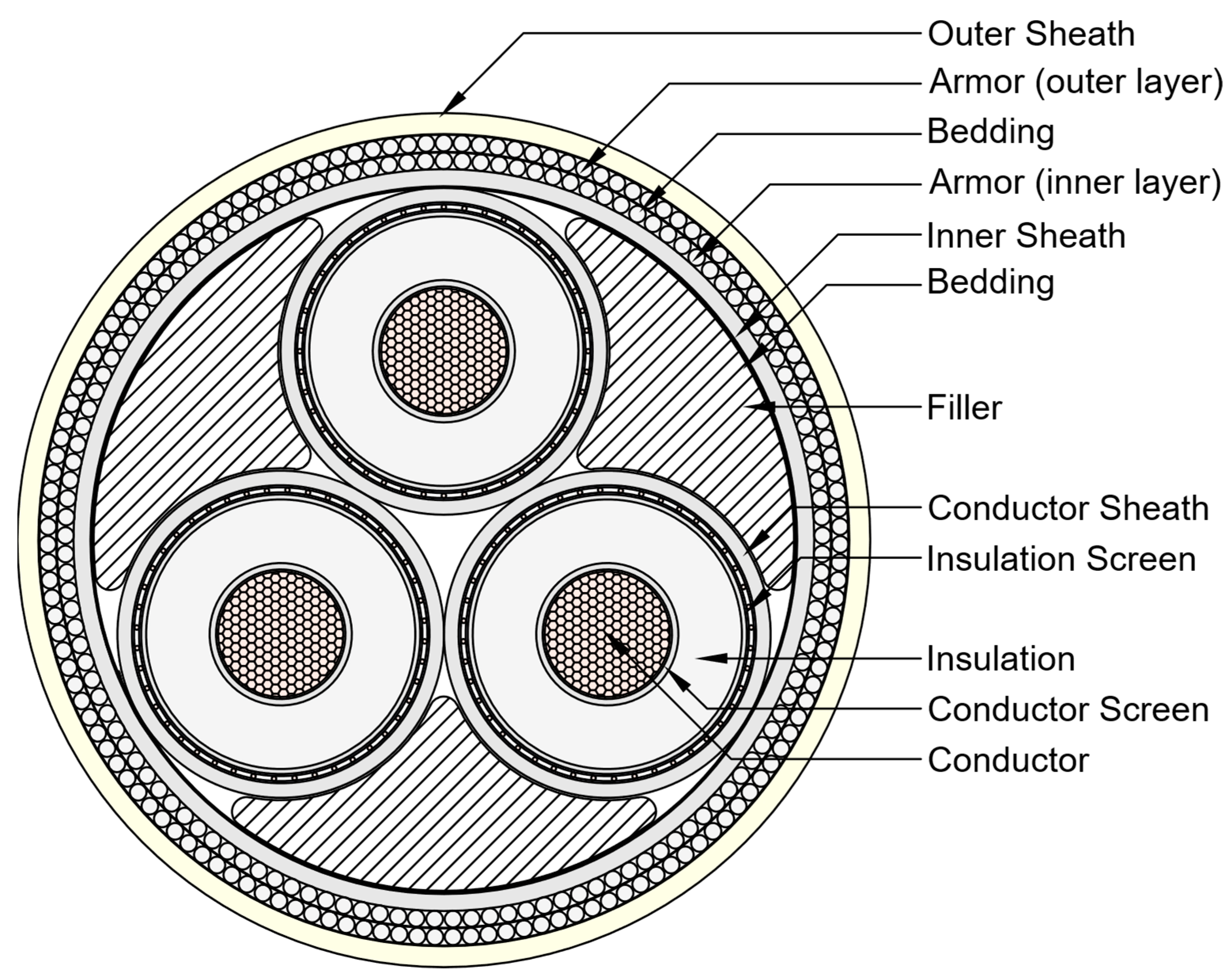
The present study provides three dynamic power cable models rated at 33 kV, 66 kV, and 132 kV. The cross-sectional view of power cable design is shown in Figure 1 and is standard for all three models. The only difference between the three models is the dimensioning of individual layers. Detailed dimensions for all three variants are given in Table 1 and Figure 2. The power cable consists of three conductor units. Each conductor unit has a nominal copper cross-section area of 630 mm2. The conductor is enclosed by a copper screen tied to the insulation layer made of cross-linked polyethylene (XLPE). XLPE insulation is preferred due to its favorable dielectric properties and high temperature resistance. Furthermore, XLPE has very good chemical and water resistance and provides very good protection against environmental degradation. Additionally, XLPE mechanical strength and low dielectric loss make it a durable and energy-efficient choice for insulation in dynamic power cable applications. The conductors are helically wound along the cable’s longitudinal axis and are separated by three filler bodies made of medium-density polyethylene (MDPE) to maintain the cable’s cross-section shape. The whole bundle is encapsulated in the inner sheath made of MDPE. The cable is protected by two cross-wound armor layers comprised of helically wound galvanized steel wires. The twist directions of the two layers are opposite to ensure the torsional balance of the cable. The 33 kV and 66 kV models use armor wire with a 3.15 mm diameter, and the 132 kV model uses armor wire with a 4.0 mm diameter. The armor layers are separated by thin bedding layers made of Polypyrrole.
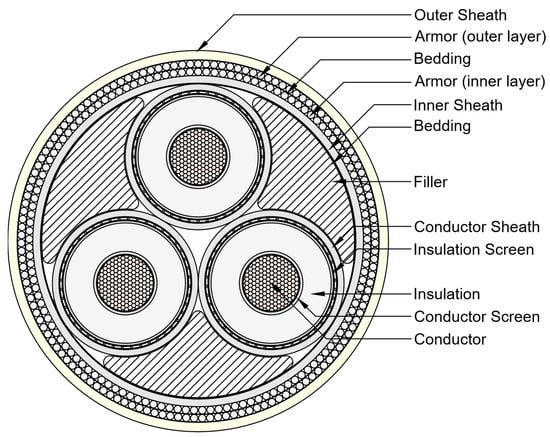
Figure 1.
Present dynamic power cable layer composition.

Table 1.
Physical properties of power cable layers and components.

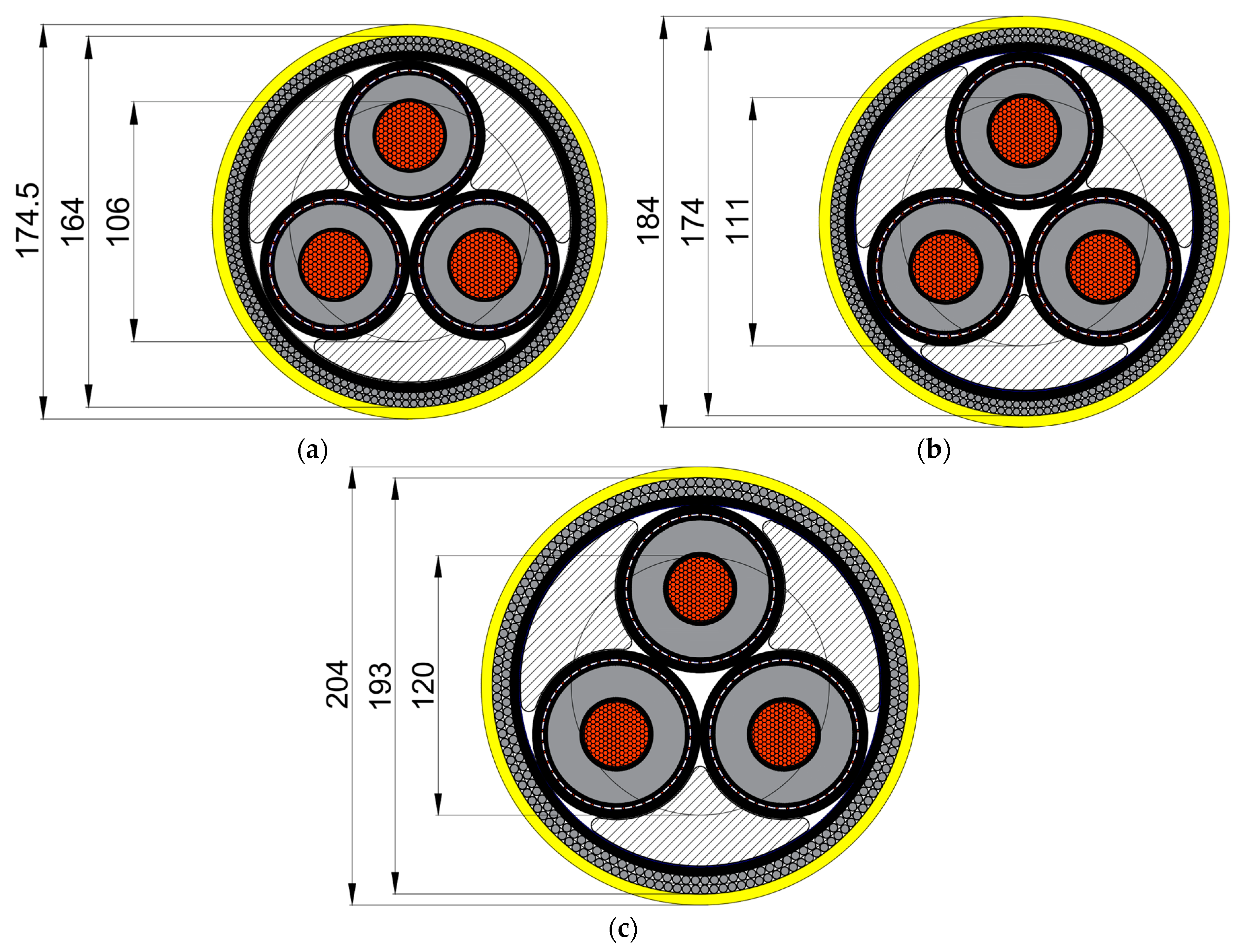
Figure 2.
Outer diameter, armor diameter, and conductor diameter for (a) 33 kV, (b) 66 kV, and (c) 132 kV cable cross sections. Dimensions given in mm.
Abrasion and elemental protection of the cable is provided by an extruded outer sheath made of high-density polyethylene. Table 2 lists material properties of power cable layers and components. Figure 2 shows the outer diameters of the three considered cable models. Additionally, the outer diameters of the armor layers and copper conductors, typically required to conduct strain calculations and fatigue analysis in the global response model, are provided. The yield strength of the wire is MPa, and the yield strength of the pure Electrolytic Tough Pitch (ETP) copper conductor is MPa. However, it should be noted that the stress elongation departs from the linear relation well below the yield point for pure copper, typically defined as a limit of 0.2% plastic strain. For ETP copper with a yield strength of MPa, the corresponding plastic limit reported by Robinson [41] is MPa. Therefore, both the stress history of the conductor wires and the armor wires should be evaluated in the power cable capacity analysis.
Table 2.
Material properties of power cable layers and components.
2.2. Numerical Model of the Dynamic Power Cable
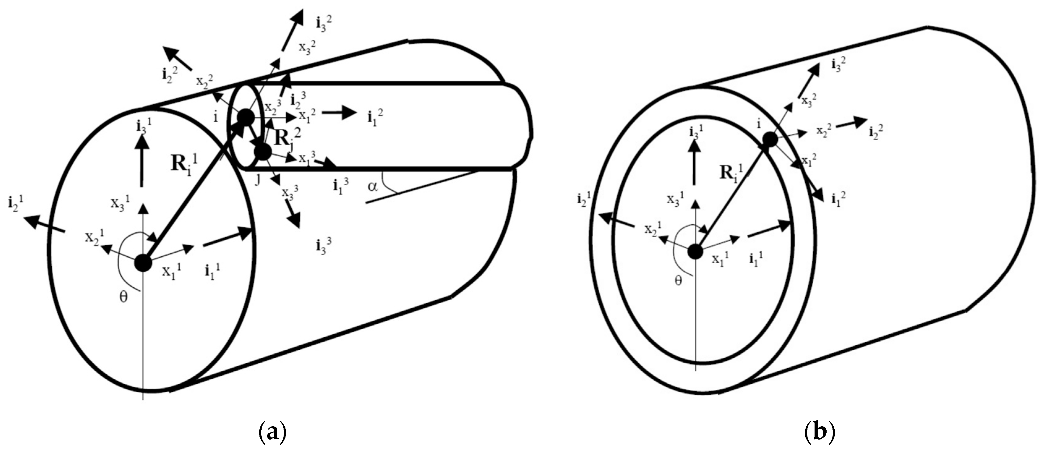
The UFLEX program was developed based on non-linear continuum mechanics, applying the finite element method (FEM) to solve the governing equations. It assumes a 2D, axisymmetric solution domain for tension, torsion, pressure, and bending loads of composite pipes and cables, enabling closed-form solutions through differential geometry. Helical elements are considered thin rods, allowing thin curved beam theory to be used by neglecting transverse strains and shear deformations. The 2D approach and thin-walled tubular assumption permit axisymmetric thin shell theory, with modifications for longitudinal strains due to helical winding. The FEM formulation employed in UFLEX is the co-rotational formulation referring all quantities to the initial configuration. The principle of the co-rotational formulation is to separate the rigid body motion from the local or relative deformation of the element, as illustrated in Figure 3a,b for beam and shell elements, respectively. It is realized by attaching a local coordinate system to the element and letting it continuously translate and rotate with the element during deformation (Sævik [16]). The solution procedure for the variational problem is based on the principle of virtual displacements. It is obtained by introducing models for kinematics description and material laws connecting strains with resulting stresses and displacement interpolation.

Figure 3.
Definition of the reference systems used in UFLEX 2D for (a) helical beam elements; (b) shell elements (SINTEF [42]).
In the UFLEX bending formulation, the helical structure elements are assumed to be thin. The implication is that transverse strains become negligible, and the theory of thin curved beams can be employed. By introducing the Euler–Bernoulli assumption, the transverse shear deformations are neglected and simplified relations for element strains can be derived. The Green–St. Venant strain tensor formulation is assumed to avoid shear locking while incorporating essential interactions between longitudinal strain and torsion. However, all terms related to coupling between longitudinal strain and torsion are included. Longitudinal differentials vanish by taking a 2D approach, significantly increasing computational efficiency. The assumption of thin-walled tubulars allows using axisymmetric thin shell theory for tubular elements. However, to consider longitudinal coupling effects resulting from the fact that the tubulars may be helically wound, modifications are made concerning the longitudinal strains utilizing the results obtained for the helical beams (SINTEF [42]).
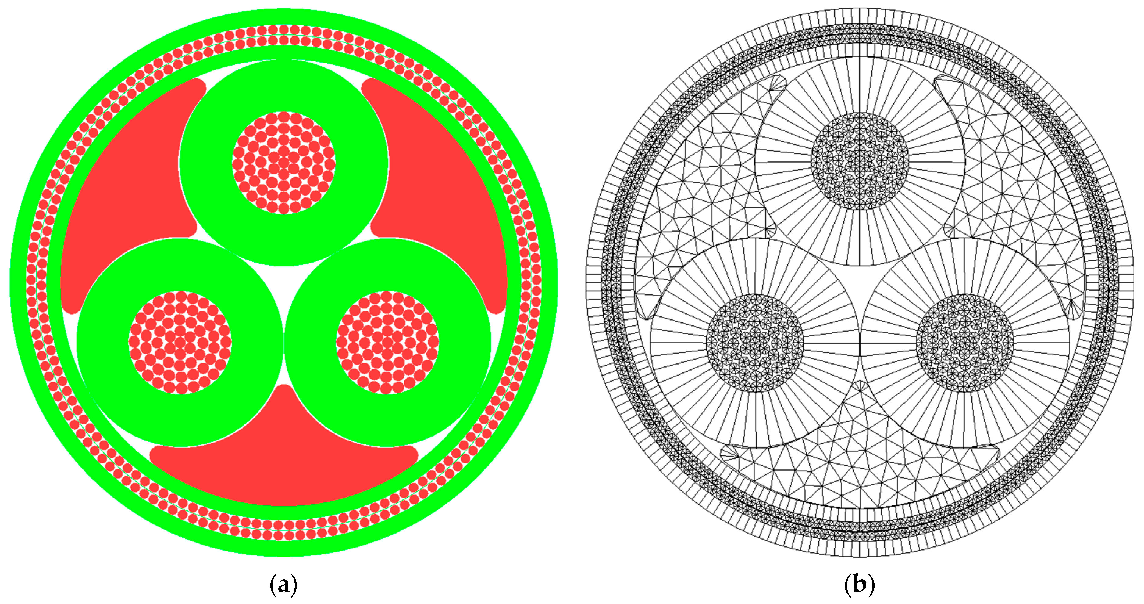
The cross-section is represented by several bodies, each modeled by tailor-made finite elements. UFLEX supports the two body types: (i) filled bodies representing components such as copper conductors, steel armor, and filler inlets; (ii) tubulars representing extruded power cable sheath or insulation layers. In UFLEX, three different element types are available to the user, i.e., beam, shell, and beamshell. The beam element applies to the filled bodies, whereas the shell element applies to the tubulars. The beamshell element is primarily used to model filled bodies allowing contraction or expansion but can also be utilized for tubulars (SINTEF [42]). Figure 4a shows the element types assigned to different components of the 66 kV power cable model investigated in the present study. The green color denotes the shell element type, and the red denotes the beam element type. The corresponding FEM mesh is visualized in Figure 4b. A detailed description of element types and simplifications (i.e., layer merging) for individual layers of the cable is presented in Table 3.
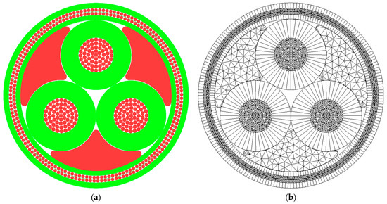
Figure 4.
Modeled 66 kV cable cross-section: (a) element types, red denotes beam elements, green denotes shell elements; (b) computational mesh view.
Table 3.
Material properties of individual layers of the reference power cable.
2.3. Mesh Sensitivity Study
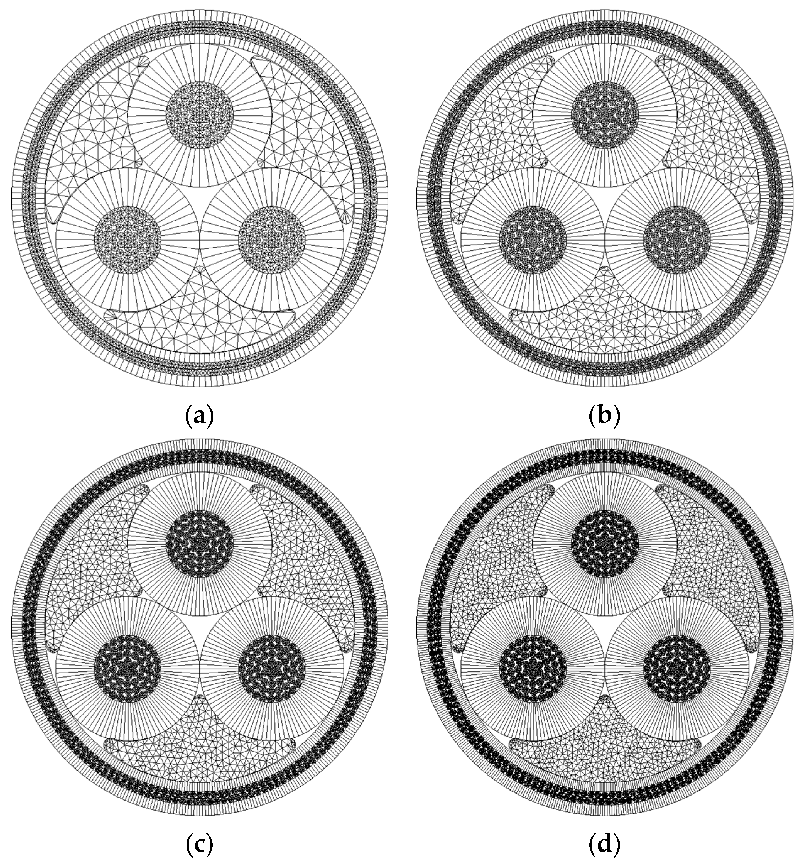
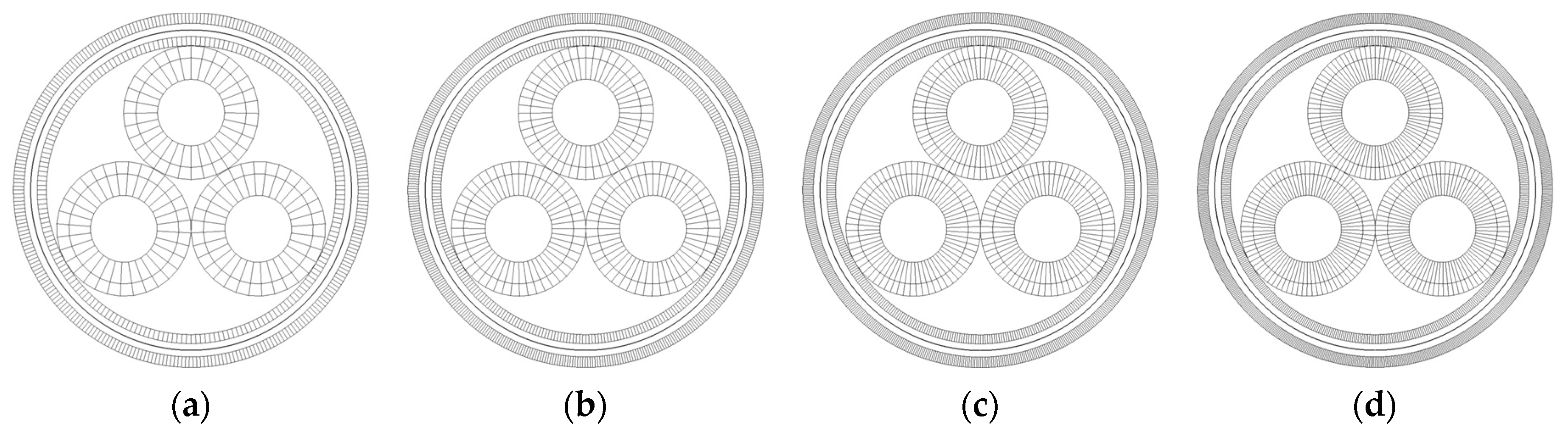
A mesh sensitivity study is an essential first step in FEM analysis. Its primary goal is to find the optimal mesh size that balances the computational efficiency with the accuracy of results. The present mesh sensitivity study involves both a global mesh density sensitivity study and an investigation of the effects of mesh refinement for the individual layers of the cable. The 66 kV cable model was selected for the mesh sensitivity study. It is assumed that the other cable variants are geometrically similar and have dimensions close enough to the 66 kV variant to generalize the results of the mesh convergence studies to 33 kV and 132 kV models. In the base case (Figure 4b), the conductor insulation and sheath layers are discretized with 48 shell elements and the cable bedding and outer sheath with 200 shell elements. Armor wires and conductor wires are discretized with 8 triangular beam elements. Triangular beam elements are used to model the filled bodies by dividing the circumference of the filler section into 44 segments. The other mesh variants, shown in Figure 5, are created using a constant mesh refinement factor. The summary of mesh parameters of the considered mesh variants is presented in Table 4.
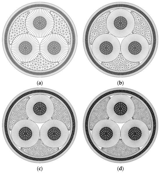
Figure 5.
Global mesh density variants: (a) very coarse, (b) coarse, (c) normal, (d) dense.
Table 4.
Parameters of mesh variants used in the mesh sensitivity studies.
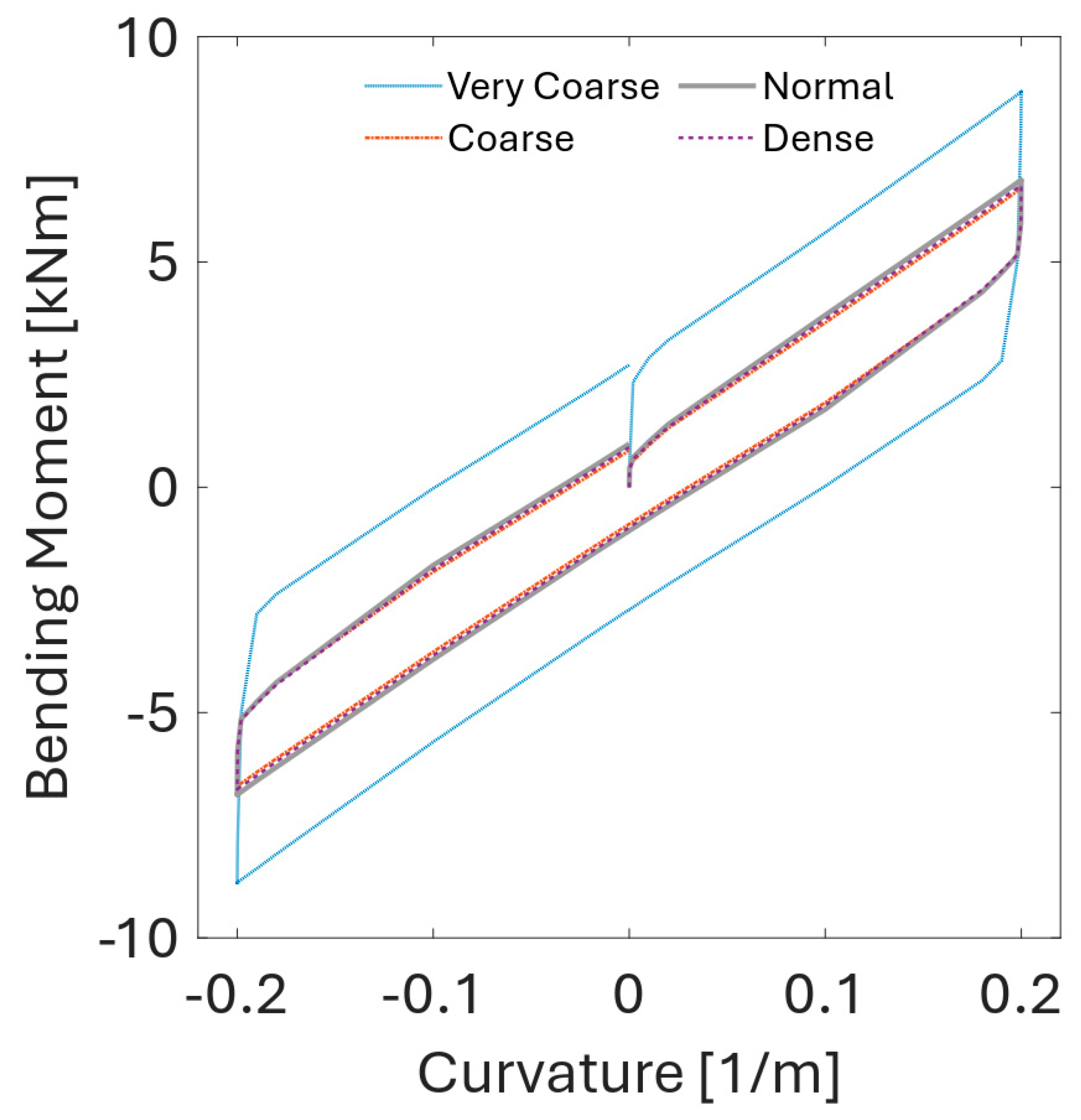
The global mesh density sensitivity study procedure involves simulations of the cyclic bending of the cable under constant tension. The cross-section is first loaded to an axial tension of 50 kN, and then cyclic bending is applied while keeping the axial tension constant. The results of the hysteretic behavior of bending moment versus curvature of the cable for different mesh variants are shown in Figure 6.
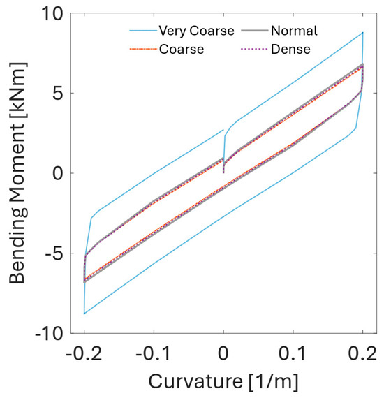
Figure 6.
Hysteretic behavior of curvature-bending moment for cases with different global mesh densities.
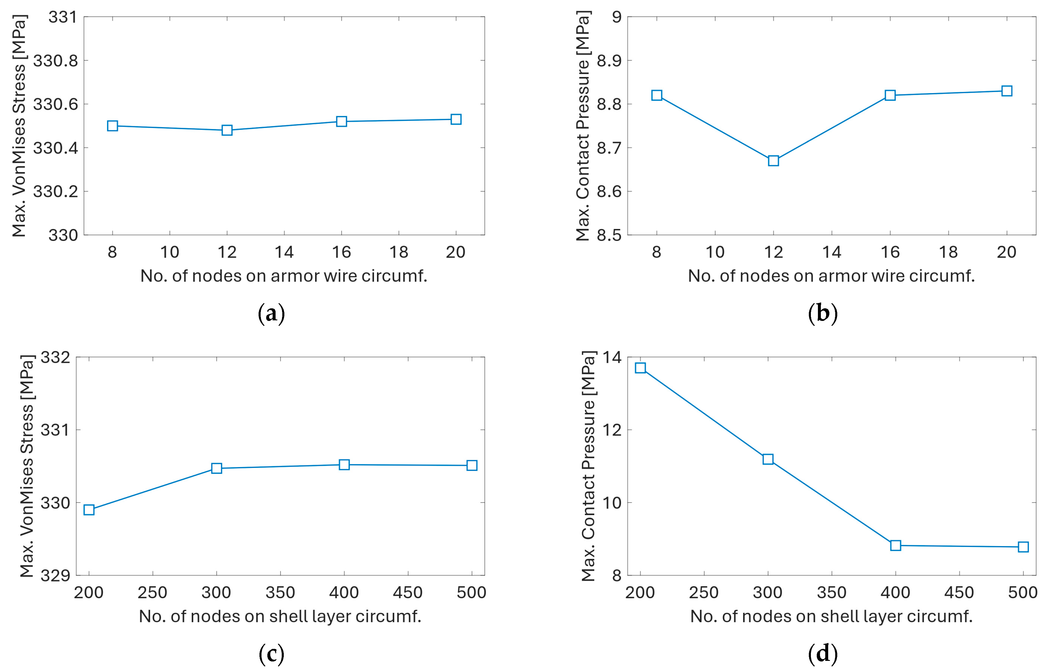
Except for the very coarse mesh variant, all the remaining mesh variants show very close agreement with respect to the slope and magnitude of the bending moment hysteresis. To further understand the influence of mesh resolution of the individual power cable layers, additional mesh sensitivity studies are carried out for sheath layers (Figure 7), and armor wires (Figure 8). The overall loading procedure is the same as in the global mesh density sensitivity study. The only difference is that the base mesh now has parameters corresponding to the normal mesh variant (see Table 4), and only the mesh of the studied component is refined. Ye and Yuan [43] showed that the model sensitivity to filler mesh refinement is very low, which is also observed in the present study. The effect of the mesh refinement on the maximum predicted Von Mises stress in the cable cross-section is shown in Figure 9a,c. Except for the coarse mesh case, the predicted stress values for other mesh variants are in close agreement. The effect of the mesh refinement on the maximum contact pressure (Figure 9b,d) between different cable layers is much more pronounced. The normal and dense mesh variants show very good agreement of predicted contact pressure values. However, significant differences are observed in simulations using coarse and very coarse meshes.
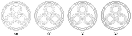
Figure 7.
Shell layers mesh variants: (a) very coarse, (b) coarse, (c) normal, (d) dense.

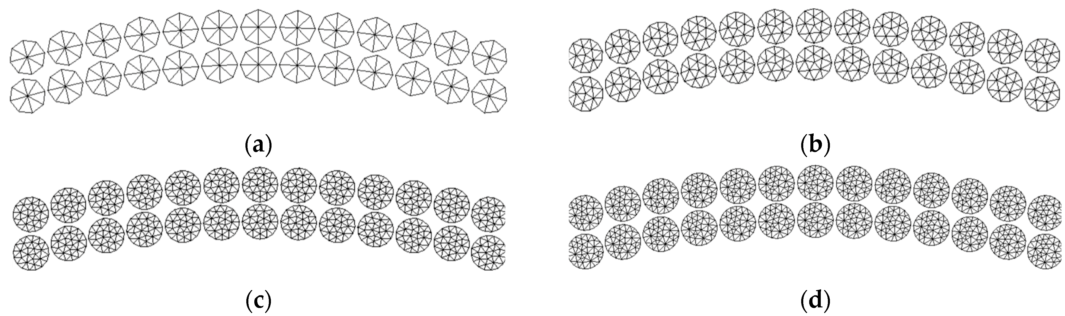
Figure 8.
Close-up view of the armor wires discretization for (a) very coarse, (b) coarse, (c) normal, and (d) dense mesh variants.
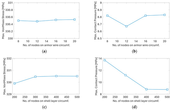
Figure 9.
Mesh sensitivity study results: (a) effect of armor wire discretization on max. Von Mises stress; (b) effect of armor wire discretization on max. contact pressure; (c) effect of shell layers discretization on max. Von Mises stress; (d) effect of shell layers discretization on max. contact pressure.
Based on the results of the mesh sensitivity studies, the normal density mesh variant is selected for further analyses, and all subsequent results are based on simulations with corresponding discretization parameters, as outlined in Table 4.
2.4. Local Analysis Results—Cable Cross-Section Properties
Mechanical properties of the three cable variants are obtained from a series of UFLEX simulations with different boundary conditions. The axial force–axial strain relation is obtained by gradually increasing the axial force and recording the axial deformation of a unit length of the cable. The obtained relations for all three power cable variants are shown in Figure 10. In all three cases, a linear relation is found with a constant slope corresponding to the axial stiffness, EA, of the cable: 622 MN for the 33 kV cable, 658 MN for the 66 kV cable, and 846 MN for the 132 kV cable variant.
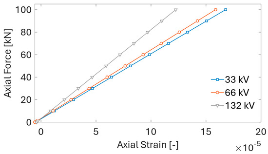
Figure 10.
Axial force–axial strain relationships for three cable variants obtained from UFLEX simulations.
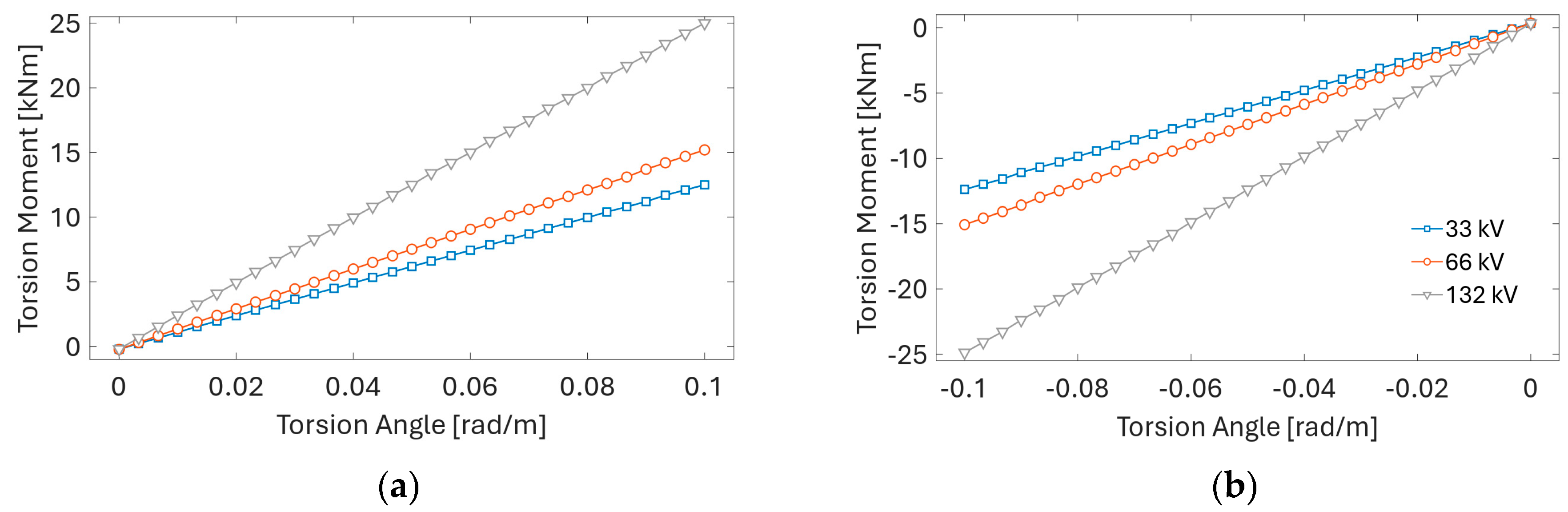
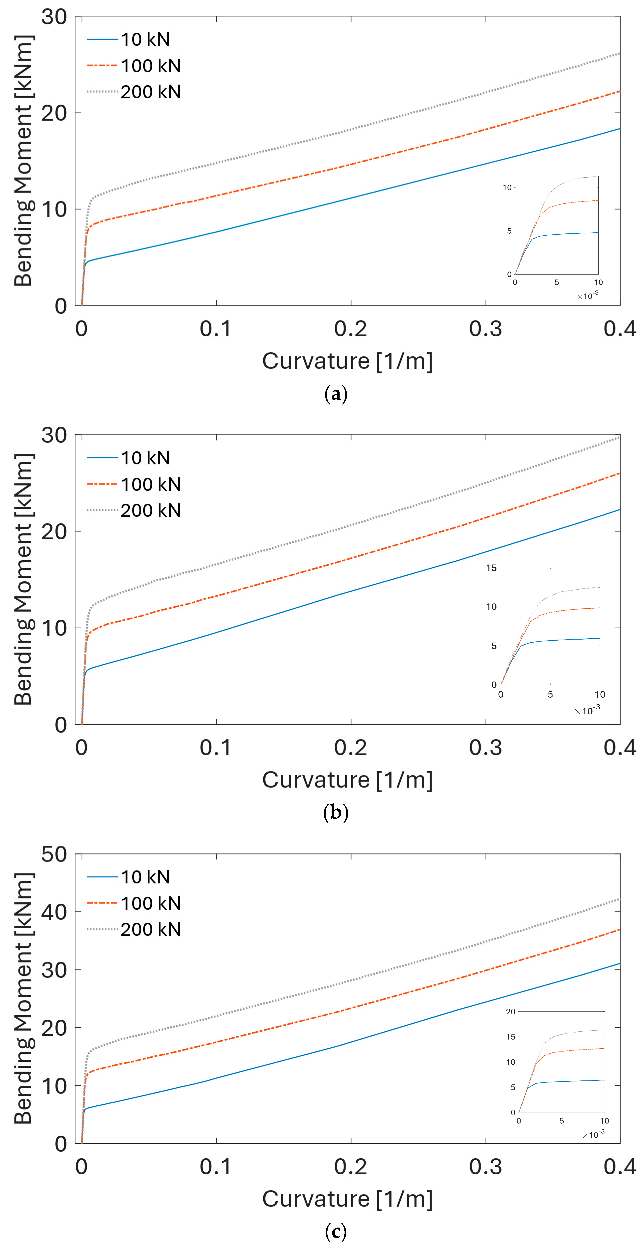
The three cable models’ torsional properties are obtained by gradually increasing rotation to a unit length of the cable and recording the resultant torsion moment. As shown in Figure 11, the torsion moment varies linearly with the applied torsion angle. The torsional stiffness, GJ, equals the slope of the corresponding line in Figure 11: 125 kNm2 for the 33 kV cable, 152 kNm2 for the 66 kV cable, and 250 kNm2 for the 132 kV cable variant. The bending moment–curvature relation is obtained by gradually loading the cable to a target tension level and subsequently subjecting it to gradually increasing curvature. As shown in Figure 12, the relation between the bending moment and curvature is not linear anymore and shows approximately a bi-linear relation.
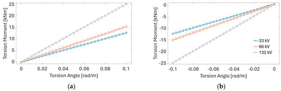
Figure 11.
Torsion angle–torsion moment relationships for three cable variants obtained from UFLEX simulations: (a) clockwise; (b) anti-clockwise rotation. Applied axial tension, 50 kN.
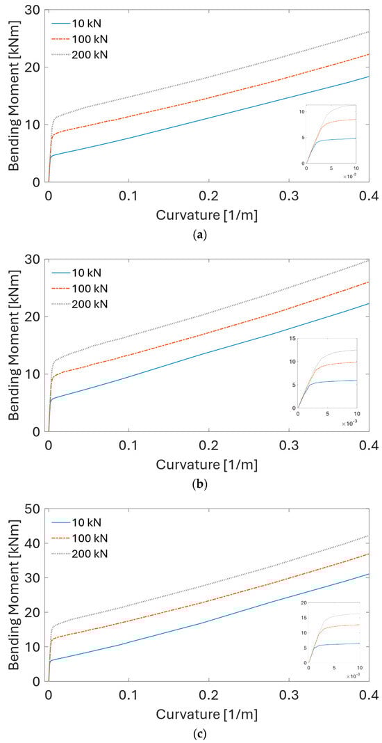
Figure 12.
Bending moment–curvature relationships for three cable variants obtained from UFLEX simulations at different tension levels: (a) 33 kV, (b) 66 kV, (c) 132 kV cable model.
It is also apparent that the cable bending stiffness changes for different tension levels. However, the slopes remain approximately the same. The slope of the first linear segment is defined as the stick stiffness of the cross-section, and the slope of the second segment is called the slipping stiffness or nominal stiffness. Stick-slip behavior in composite cables arises as different layers with unique material properties alternately stick and slip over each other under cyclic loading due to varying frictional forces at their interfaces. This cycle of sticking and slipping is driven by the tension and compression from environmental forces acting on the power cable. The curvature at which the stiffness changes its slope is defined as the slipping curvature (Guo and Ye [44]). Once the applied load exceeds the static friction threshold, the layers begin to slip relative to each other, moving into a state of dynamic friction, which is lower. This shift reduces the resistance to movement between the layers, leading to a decrease in the overall stiffness of the cable assembly.
3. Case Study
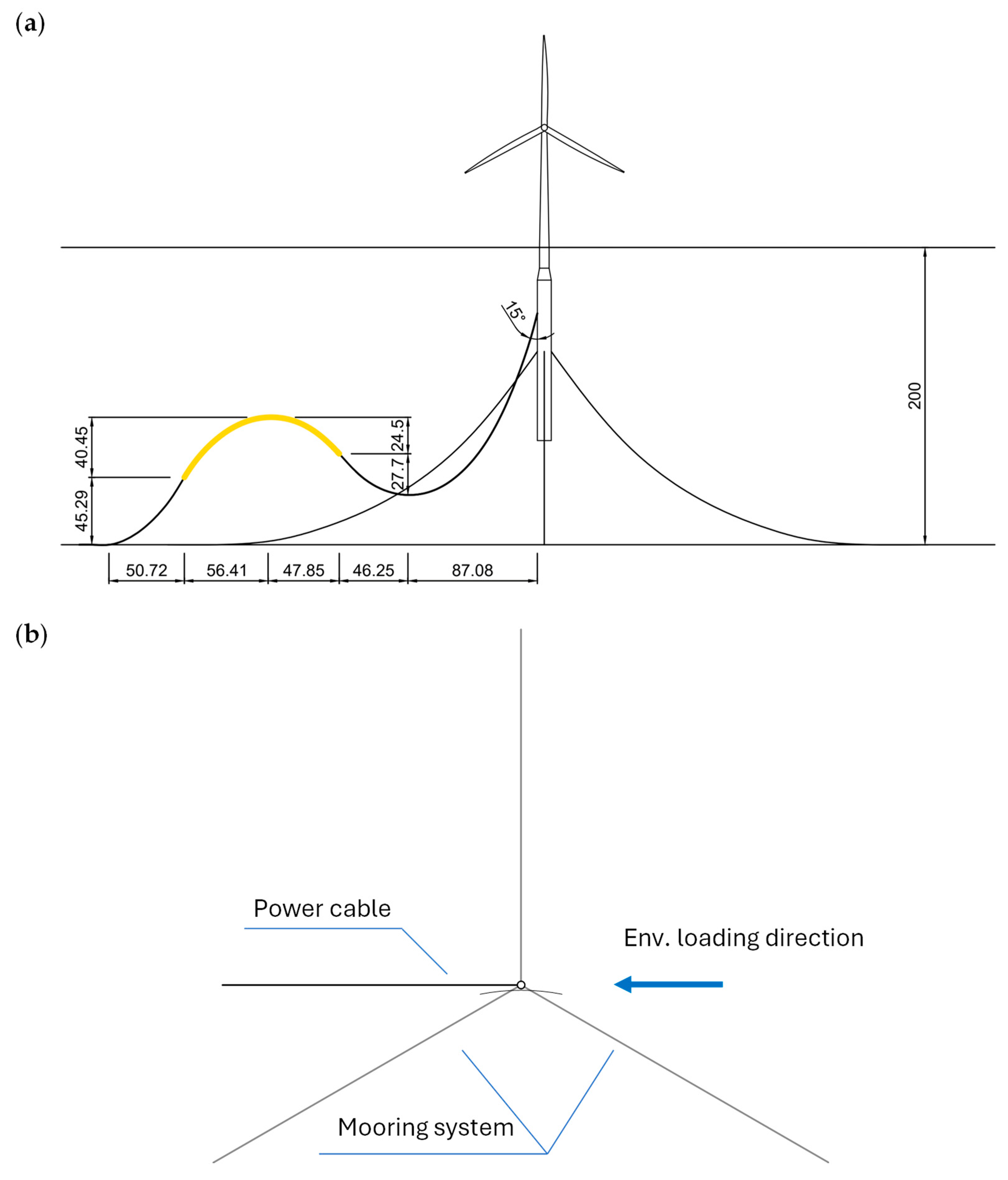
The application of the reference power cable is exemplified by presenting a case study employing the 66 kV power cable in a lazy wave configuration connected to the OC3 5MW reference wind turbine (Jonkman et al. [45]). Figure 13 presents the elevation and plan views of the considered configuration. The lazy wave configuration of the power cable is composed of three sections: two sections of bare power cable and one section of power cable with attached distributed buoyancy modules which form the hog bend, as shown in Figure 13a. The lazy wave configuration is designed based on the analytical algorithm by Zhao et al. [46]. The cable hang-off point is located 30 m below the still water level. A summary of the FOWT and power cable parameters used as inputs to coupled aero–servo–hydro–elastic time domain simulations is given in Table 5.
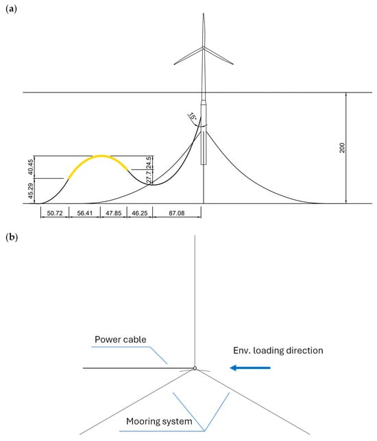
Figure 13.
Definition of the FOWT–power cable system under consideration: (a) front view, (b) plan view. Dimensions are in m.
Table 5.
Summary of the main parameters of the considered coupled FOWT-power cable system.
The global dynamic analysis in the present study is performed using OrcaFlex version 11.3a (Orcina [47]). The cable is modeled using FEM beam elements with specified axial, bending, and torsional stiffness. The non-linear mechanical properties of the cable are imported from UFLEX and given in tabularized format as an input to OrcaFlex.
The cable’s total length is 530 m, which is discretized into 530 elements with a uniform size of 1 m. The OC3 5MW spar-type FOWT model used in the present study was previously validated by Schnepf et al. [48] and Ahmad et al. [49]. An implicit solver is employed in the time-domain simulations with a fixed time step set to 0.05 s.
3.1. Environmental Conditions
Three simulations with random seeds are performed for each environmental loading condition (EC) case. Each simulation has a duration of 3 h. The environmental conditions applied in this study, listed in Table 6, are based on the joint probability model of wind speed, significant wave height and wave peak period by Johanessen et al. [50], representative of a North Sea location. The wind, wave, and current are aligned, and their heading is 90°, which is colinear with the power cable orientation. The rotor is facing the incoming wind field. The heading is selected based on the study by Zhao et al. [46] who showed that such heading is critical for the dynamic response of the cable. The 1 h mean wind velocities and the corresponding most probable significant wave heights () and wave peak periods () are selected to cover the operating range of the wind turbine (below rated, rated, above rated) and the extreme 50-year storm case above the cut-out wind speed where the wind turbine is in parked condition. The selected conditions in Table 6 do not correspond to a full set of conditions for fatigue analysis. However, they can be regarded as a range of realistic conditions that give indicative values of expected fatigue life under different load combinations. According to Johanessen et al. [50], the marginal distribution of follows a two-parameter Weibull distribution described by the cumulative distribution function:
where and are the shape and scale parameters, respectively. The wind speed at wind turbine hub is calculated using the power law formulation of wind shear:
where z is the height of the wind turbine hub above mean sea level, and is the power law exponent, which is set to 1/7 according to IEC 61400-3-1 [51]. The conditional distribution of given a (i.e., ) follows a two-parameter Weibull distribution. The expected value of given can be calculated as follows:
where and are the shape and scale parameters, respectively. The conditional distribution of given and (i.e., ) follows a log-normal distribution. Its expected value can be calculated using the following equation:
Table 6.
Summary of environmental loading conditions.
A three-parameter JONSWAP wave spectrum is applied in the dynamic simulations to model the random wave field:
where , for , and for . The JONSWAP spectrum is determined using the significant wave height , the spectral peak period , and the non-dimensional peak shape parameter γ. In the present simulations, γ = 2.87. The three-dimensional turbulent wind field data are generated by TurbSim (NREL [52]). The current profile is modeled according to the DNV-RP-C205 [53]. The tidal current velocity across the water column is modeled as a simple power law, assuming a unidirectional current:
where is the tidal current velocity at the still water level, z is the distance from the still water level, d is the water depth to the still water level, and is the exponent set to = 1/7. The surface tidal current profile is set up according to Ahmad et al. [49]. The surface tidal current speed is 0.2 m/s in all ECs, which is selected based on the NORSOK [54] standard. The variation in wind-generated current is taken as a linear profile from to still water level,
where is the wind-generated current velocity at the still water level, and m is the reference depth for wind-generated current. For the seafloor contact, the friction coefficient of 0.5 is used for the seabed in-plane friction calculation in OrcaFlex.
3.2. Global Response of the FOWT
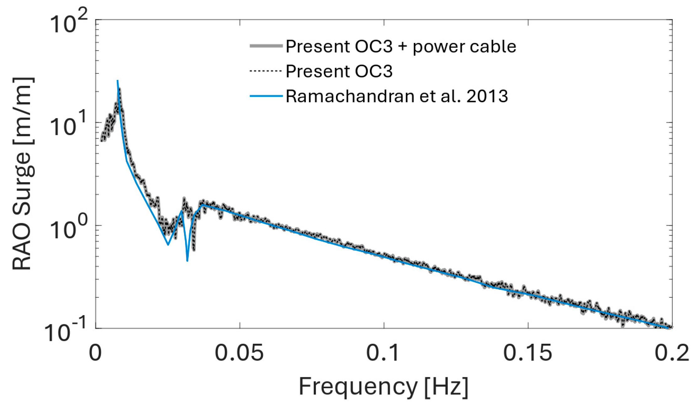
The influence of the power cable on the global response characteristic of the FOWT is analyzed by comparing the spectral response of an OC3 FOWT with and without an attached power cable. Spectral response is calculated from time-domain simulations of the two configurations at rated wind speed and subject to wave field generated from a truncated white noise spectrum. The analyzed frequency bandwidth is set from 0.002 to 0.2 Hz. The calculated responses from time-domain simulations are transformed into the frequency domain using a fast Fourier transform (FFT). Figure 14, Figure 15, Figure 16, Figure 17 and Figure 18 show the obtained response amplitude operators (RAO) for different degrees of freedom.
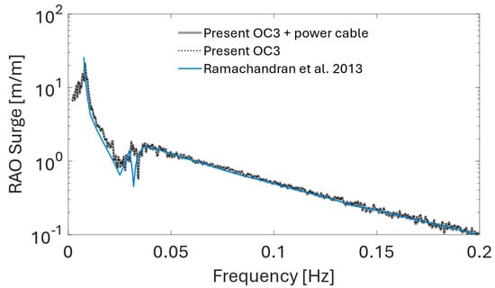
Figure 14.
Surge RAO comparison for the considered OC3 FOWT setup without and with 66 kV power cable in a lazy wave configuration. Validation against FAST simulation results by Ramachandran et al. [55].
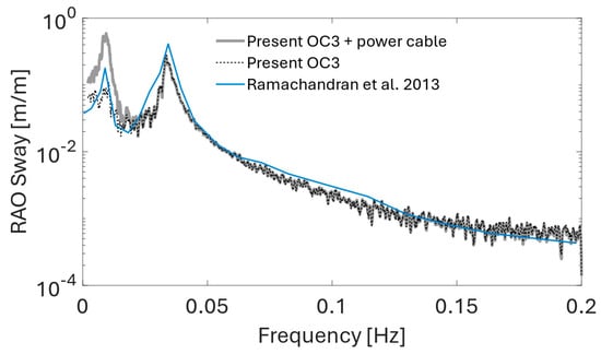
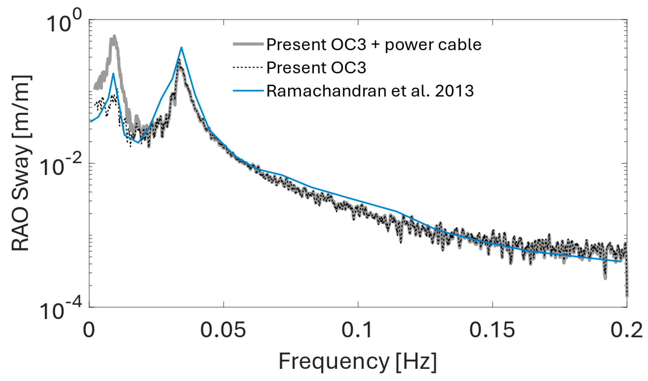
Figure 15.
Sway RAO comparison for the considered OC3 FOWT setup without and with 66 kV power cable in a lazy wave configuration. Validation against FAST simulation results by Ramachandran et al. [55].
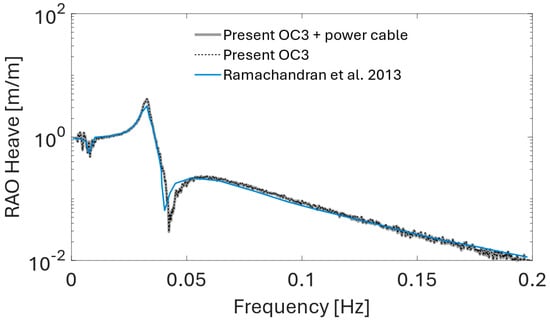
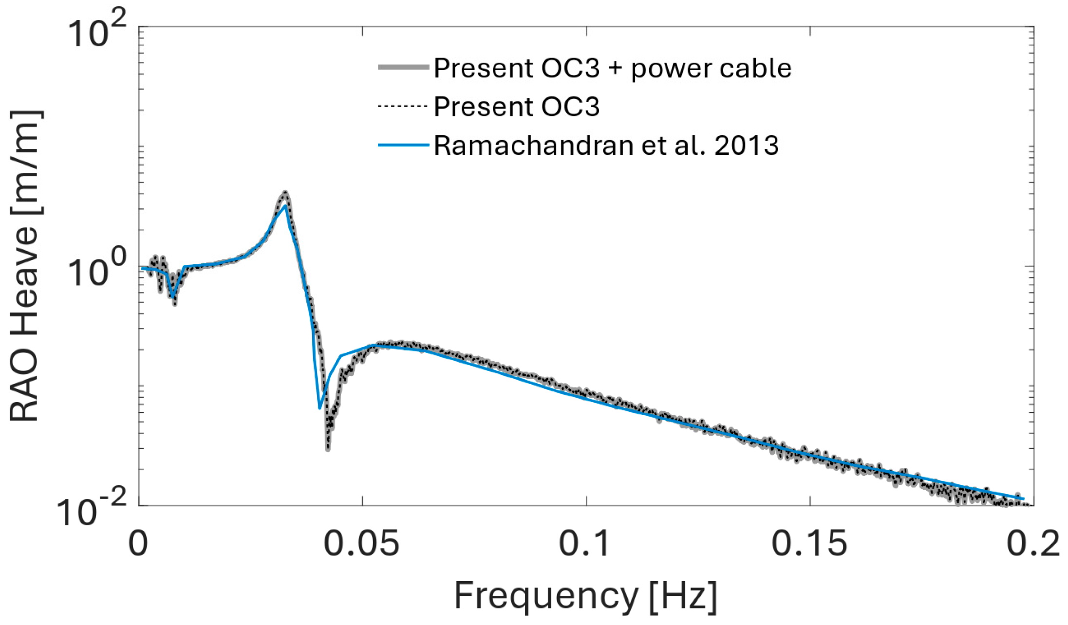
Figure 16.
Heave RAO comparison for the considered OC3 FOWT setup without and with 66 kV power cable in a lazy wave configuration. Validation against FAST simulation results by Ramachandran et al. [55].
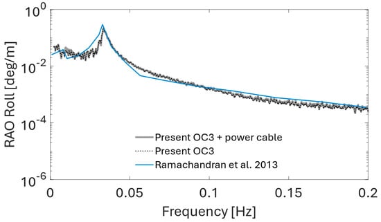
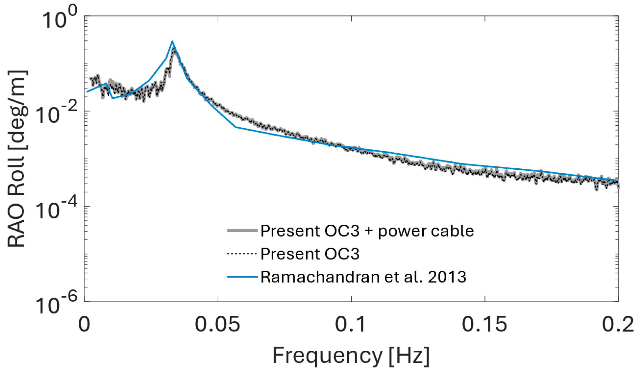
Figure 17.
Roll RAO comparison for the considered OC3 FOWT setup without and with 66 kV power cable in a lazy wave configuration. Validation against FAST simulation results by Ramachandran et al. [55].
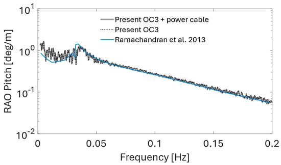
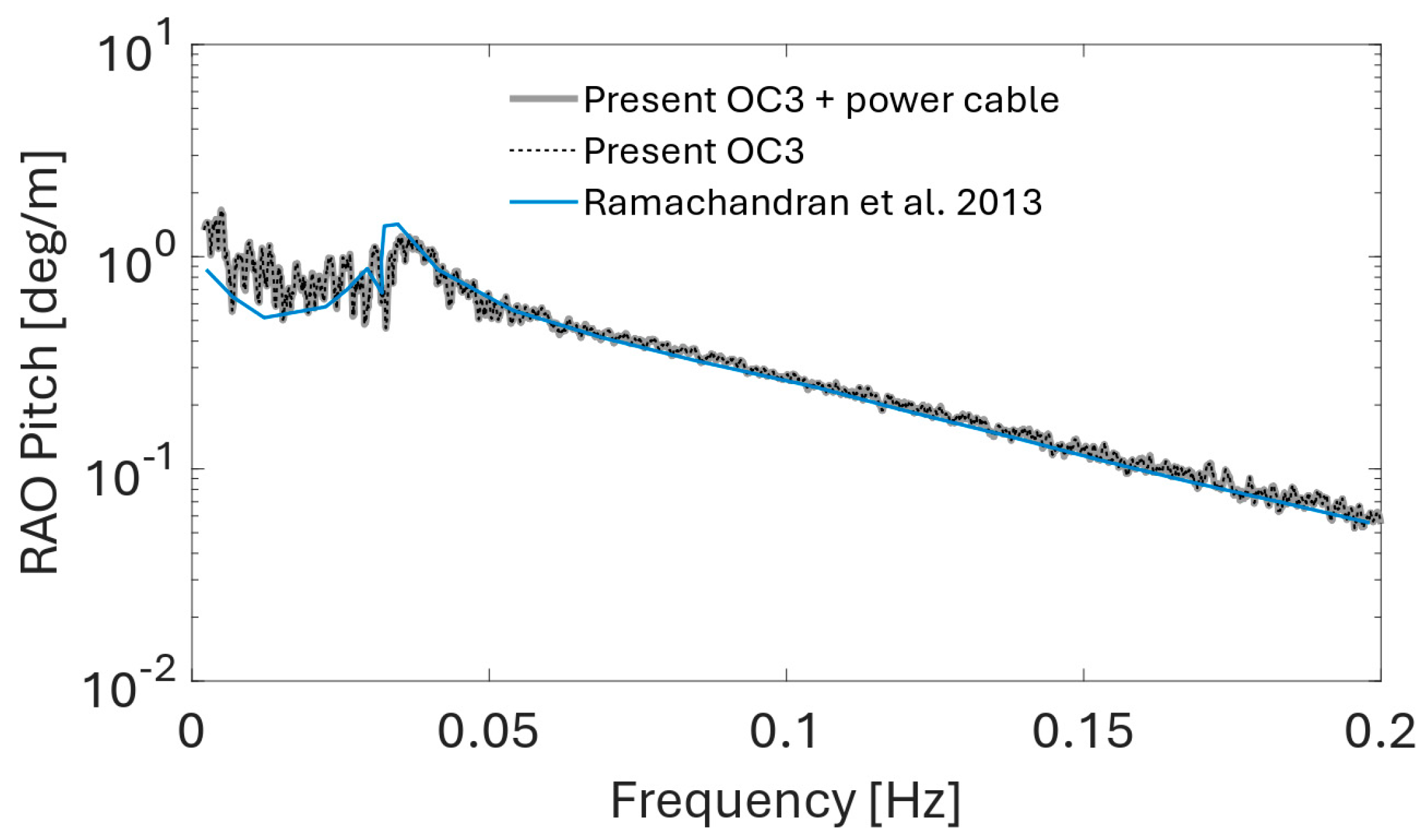
Figure 18.
Pitch RAO comparison for the considered OC3 FOWT setup without and with 66 kV power cable in a lazy wave configuration. Validation against FAST simulation by Ramachandran et al. [55].
The calculated RAOs are compared with the RAOs obtained by Ramachandran et al. [55] to validate the present model. A good match is found between the present RAOs and the reference values computed with the NREL FAST v18 software. For the present model with and without the power cable coupled with the floating turbine, the only degree of freedom where a significant difference in the RAOs is observed is the sway motion, as shown in Figure 15. The cable presence amplifies the FOWT response in sway in the low-frequency range with a spectral peak at approximately 0.01 Hz. Schnepf et al. [48] made a similar observation for the fully suspended inter-array power cable configuration. The remaining RAOs appear to be unaffected by the cable presence in the present setup.
3.3. Extreme Loading Conditions
The most accurate approach to predict the action effects in the ultimate limit state (ULS) and fatigue limit state (FLS) is the full long-term analysis, where all possible environmental conditions are considered to obtain the long-term response distribution. However, the full long-term analysis is beyond the scope of the present study. The survival scenario (EC50X in Table 6) for the present case study is a simplified case, where 50-year return period values for the wind speed, , and are obtained from the joint probability distribution described in Section 3.1.
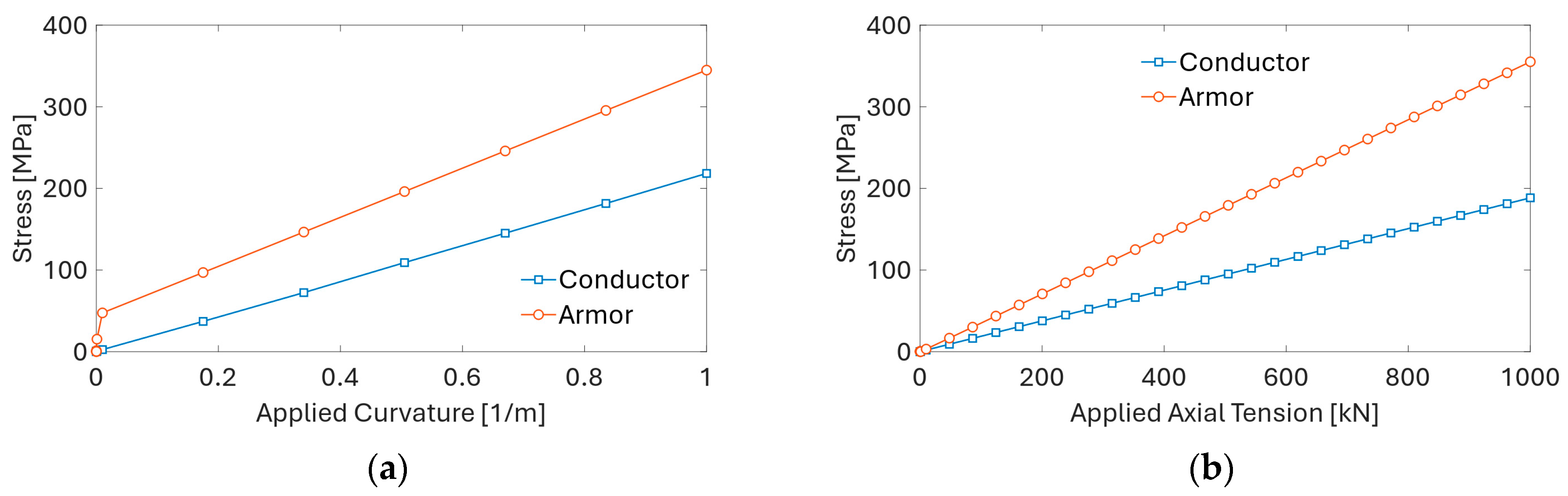
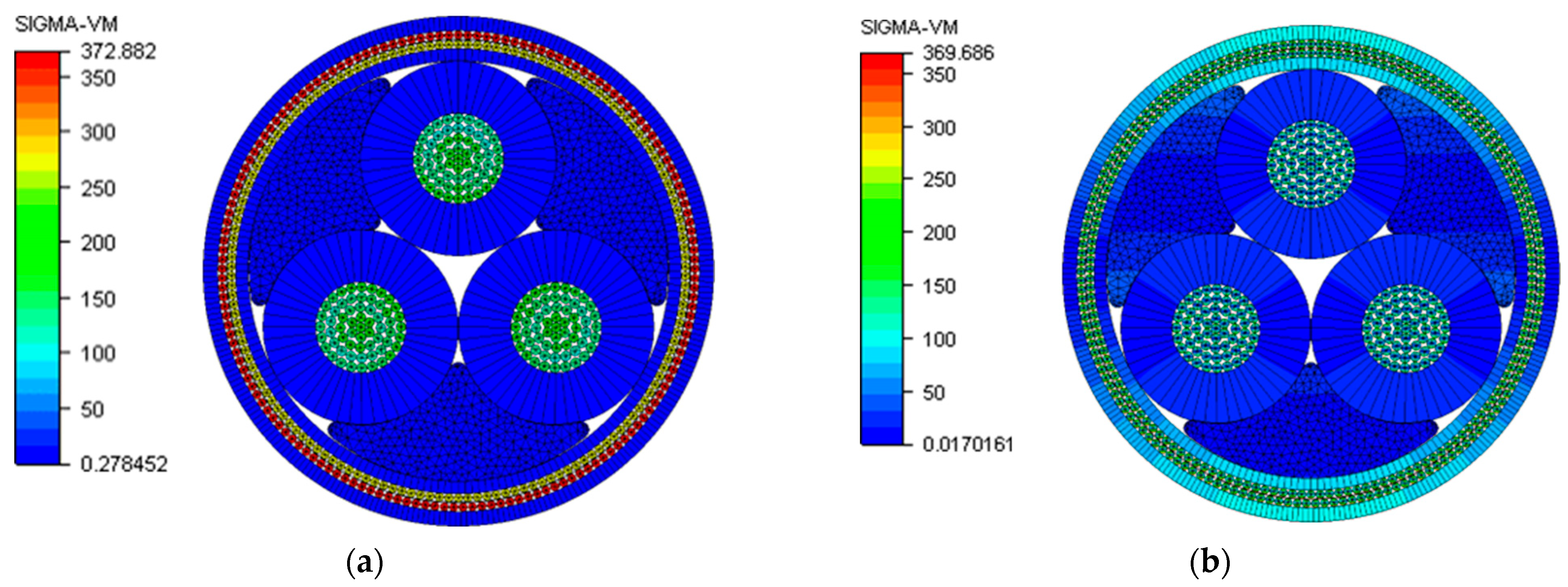
The capacity of the cable is defined by the combination of axial tension and bending curvature, which governs the allowable utilization of the cable’s components. Based on the Von Mises stress distribution in the cross-section of the cable, it is possible to establish allowable capacity curves by inspecting the utilization of material yield stress for different components. In order to obtain the limiting values of tension and curvature, the present UFLEX model is used to simulate the power cable under the axial load and the bending load until the yield strength of the armor wires or the plastic limit of the conductor wires is achieved. Figure 19 shows the stress factors for conductor and armor wires obtained from the UFLEX simulations. The results of the two limiting cases of pure axial load (Figure 20a) and pure bending (Figure 20b) indicate that the governing factor for the cable’s capacity curve is the plastic limit of the copper conductor. The value of the axial force at which the armor wires yield is approximately 1000 kN, but the plastic limit of the copper conductor is reached at approximately 600 kN. In the case of limiting curvature, the armor wires yield at about 1 rad/m, and the copper conductor exceeds the plastic limit at 0.5 rad/m.
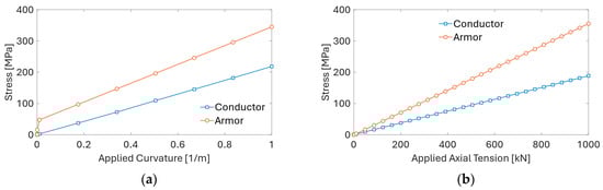
Figure 19.
Stress factors for conductor and armor wires obtained from UFLEX simulations: (a) stress versus applied curvature; (b) stress versus applied tension.
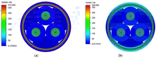
Figure 20.
Von Mises stress distribution in the cable cross-section under (a) axial load of 1000 kN, (b) bending curvature of 1 rad/m.
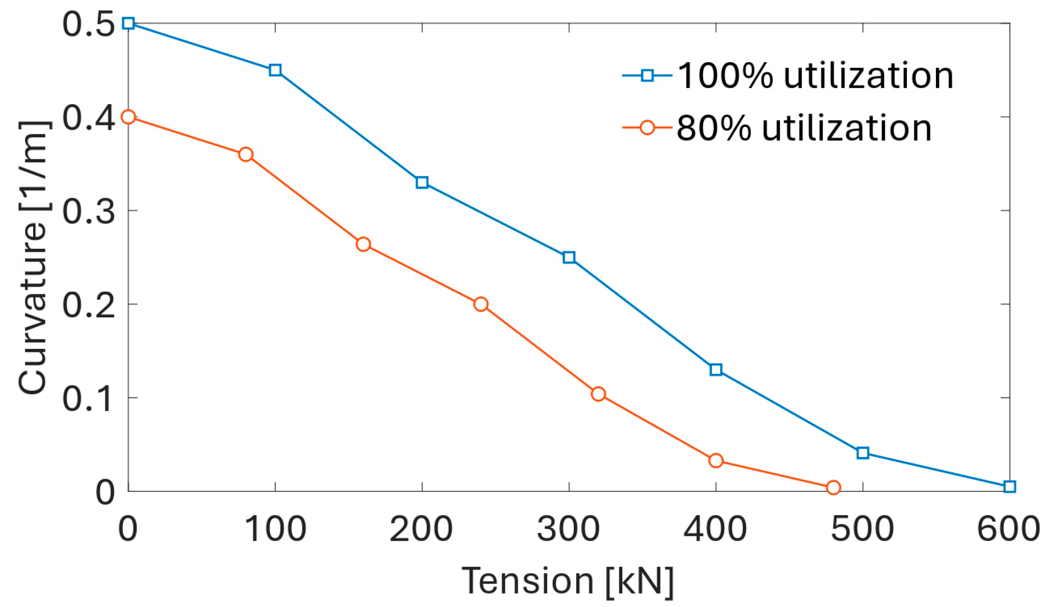
By considering additional cases of combined tension and curvature load, the capacity curve of the cable is obtained, as shown in Figure 21. The 100% utilization limit is applicable for the installation phase and the Accidental Limit State (ALS). For the extreme loading condition, the 80% utilization curve is applicable for an Ultimate Limit State (ULS). The Minimum Bending Radius (MBR) is defined as the reciprocal of the curvature limit at zero tension on the 100% utilization curve. Conversely, the Maximum Handling Tension (MHT) is defined as the tension limit at zero bending.
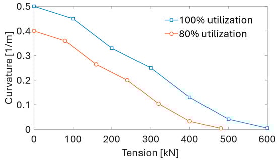
Figure 21.
Capacity curves for the 66 kV cable variant.
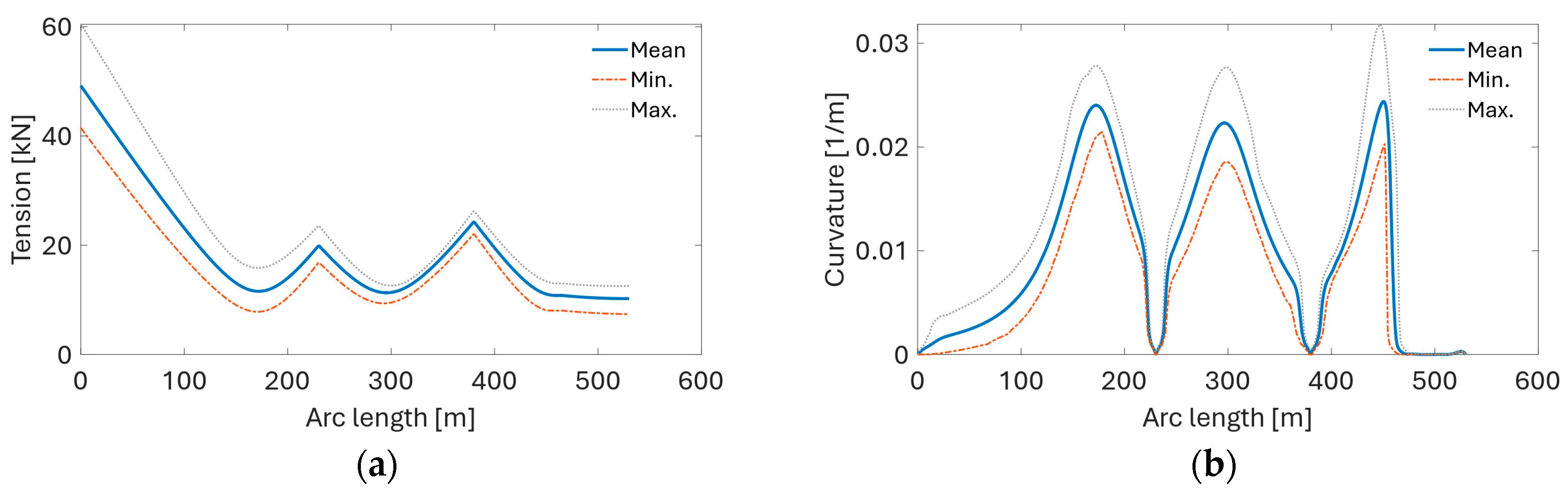
The effective tension and curvature envelopes for the extreme loading condition with a 50-year return period are shown in Figure 22. The maximum values of tension and curvature remain well within the safe operational limits of the cable and do not exceed the ultimate limit state criteria during the simulated 50-year storm conditions.
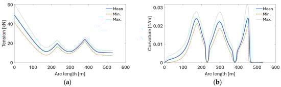
Figure 22.
Power cable response under 50-year storm extreme condition: (a) effective tension envelope, (b) curvature envelope.
3.4. Dynamic Simulations
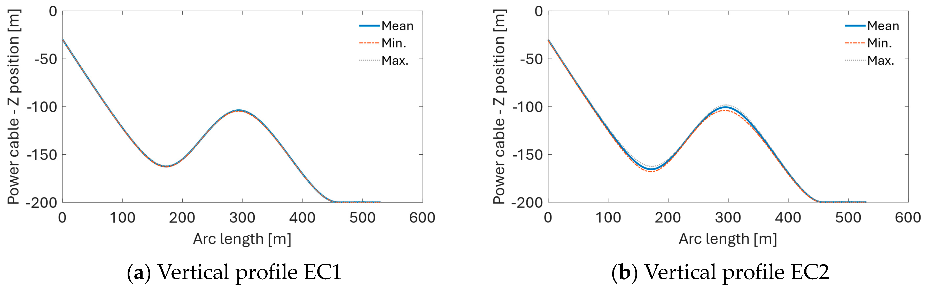
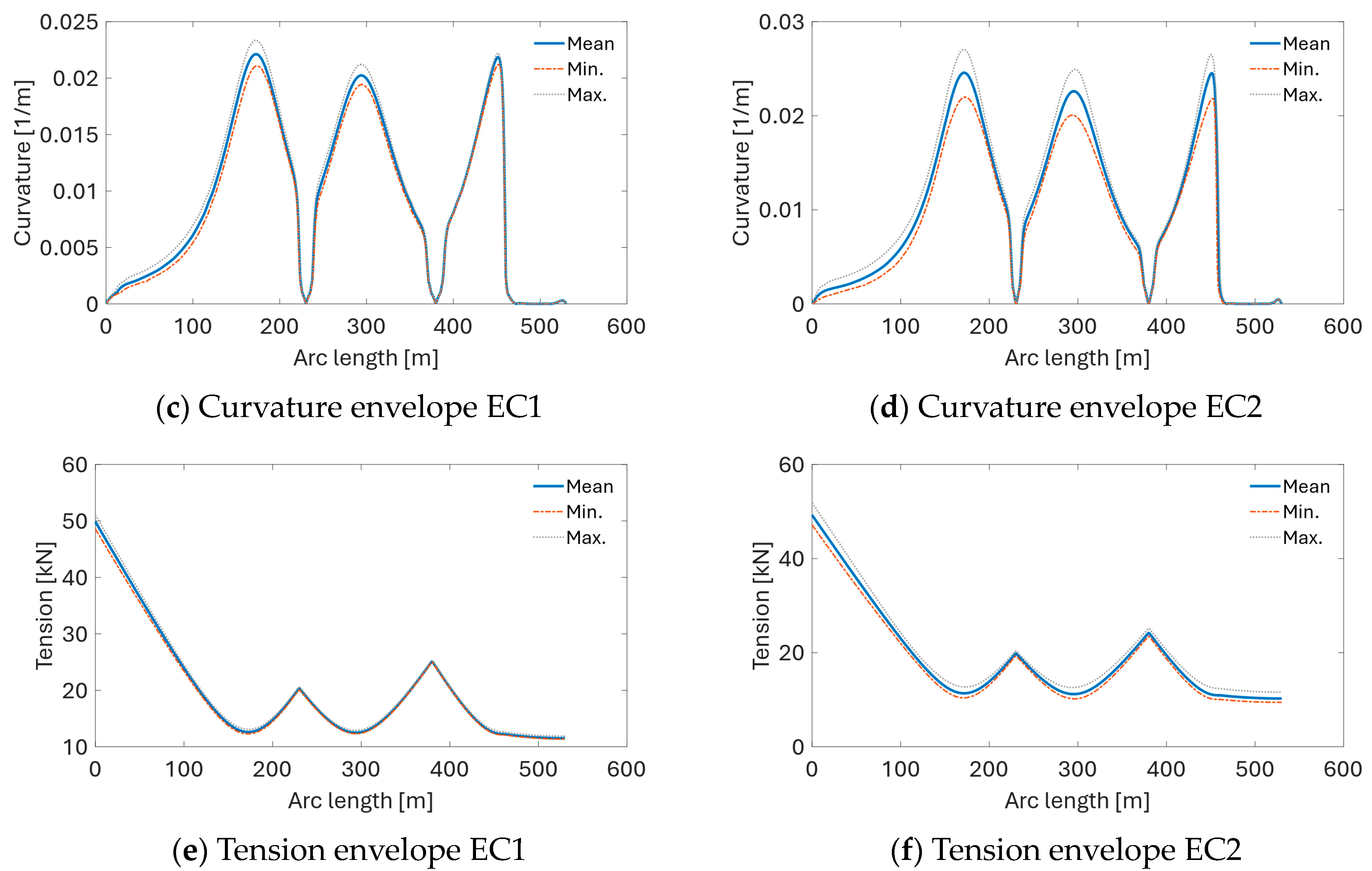
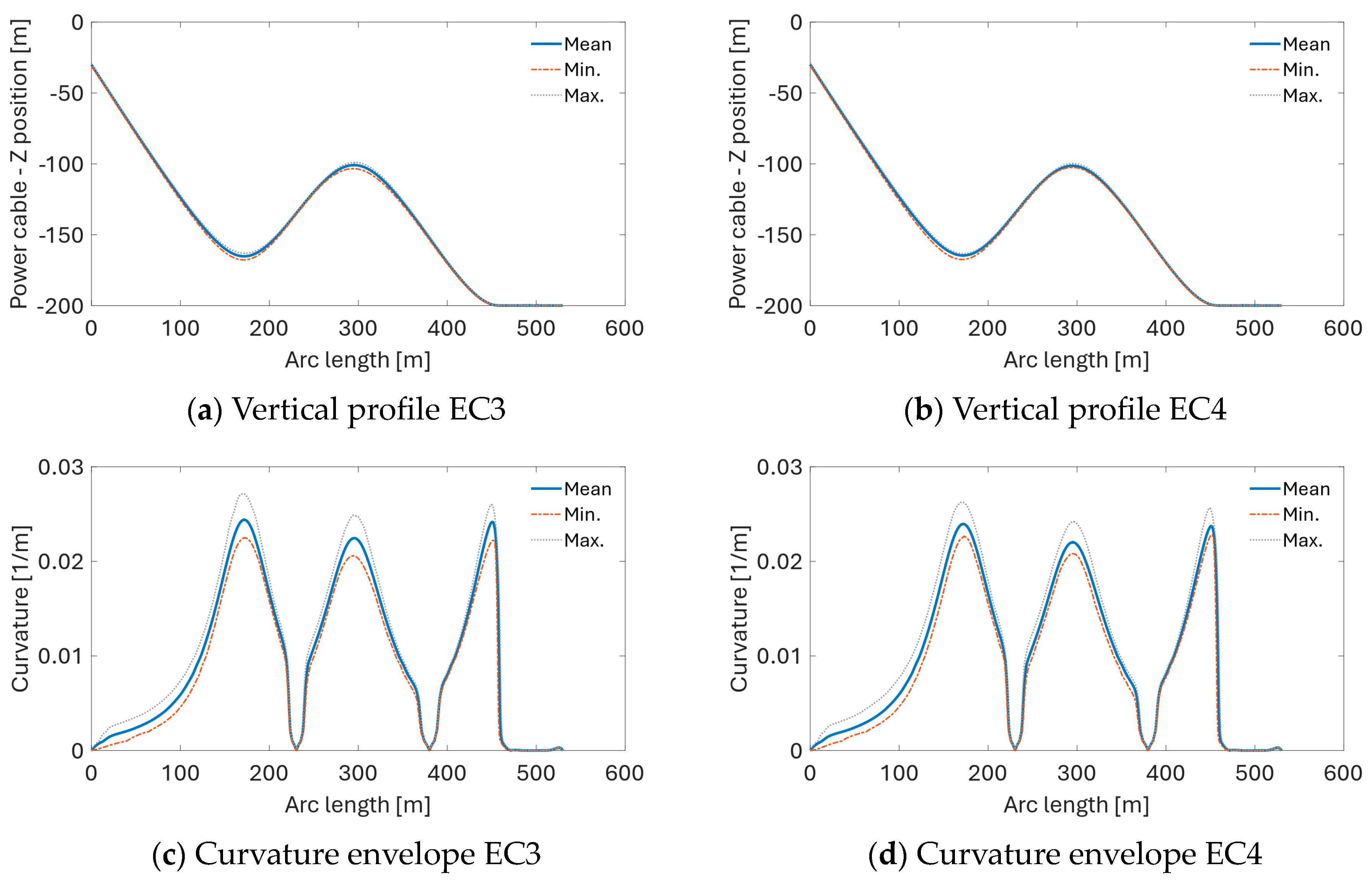
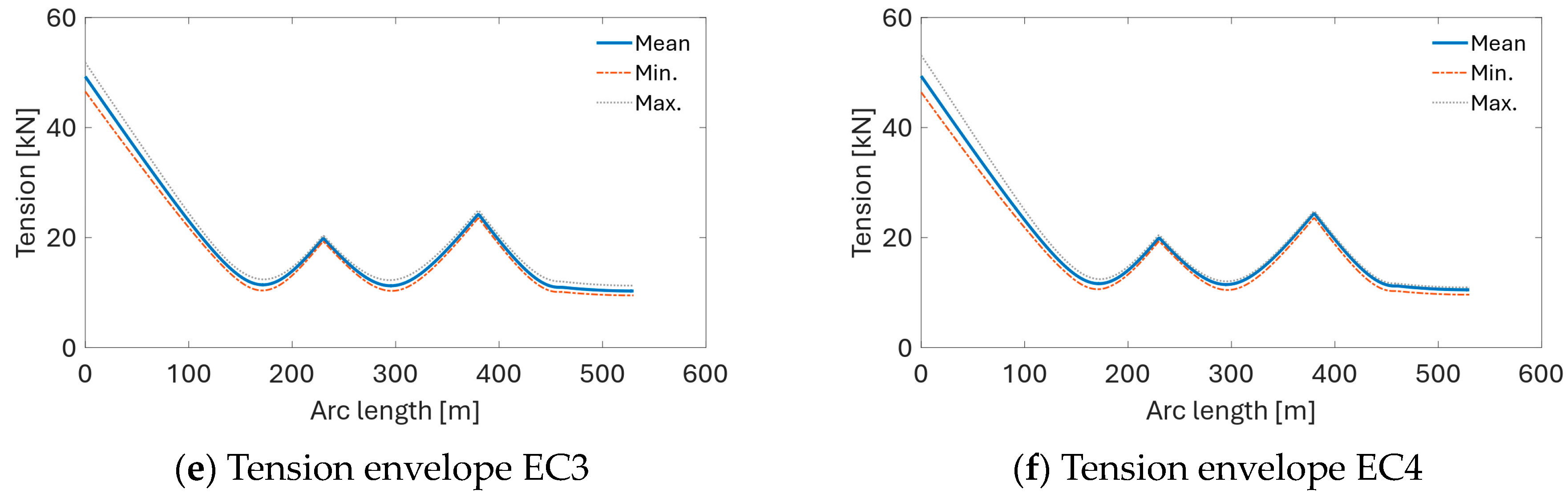
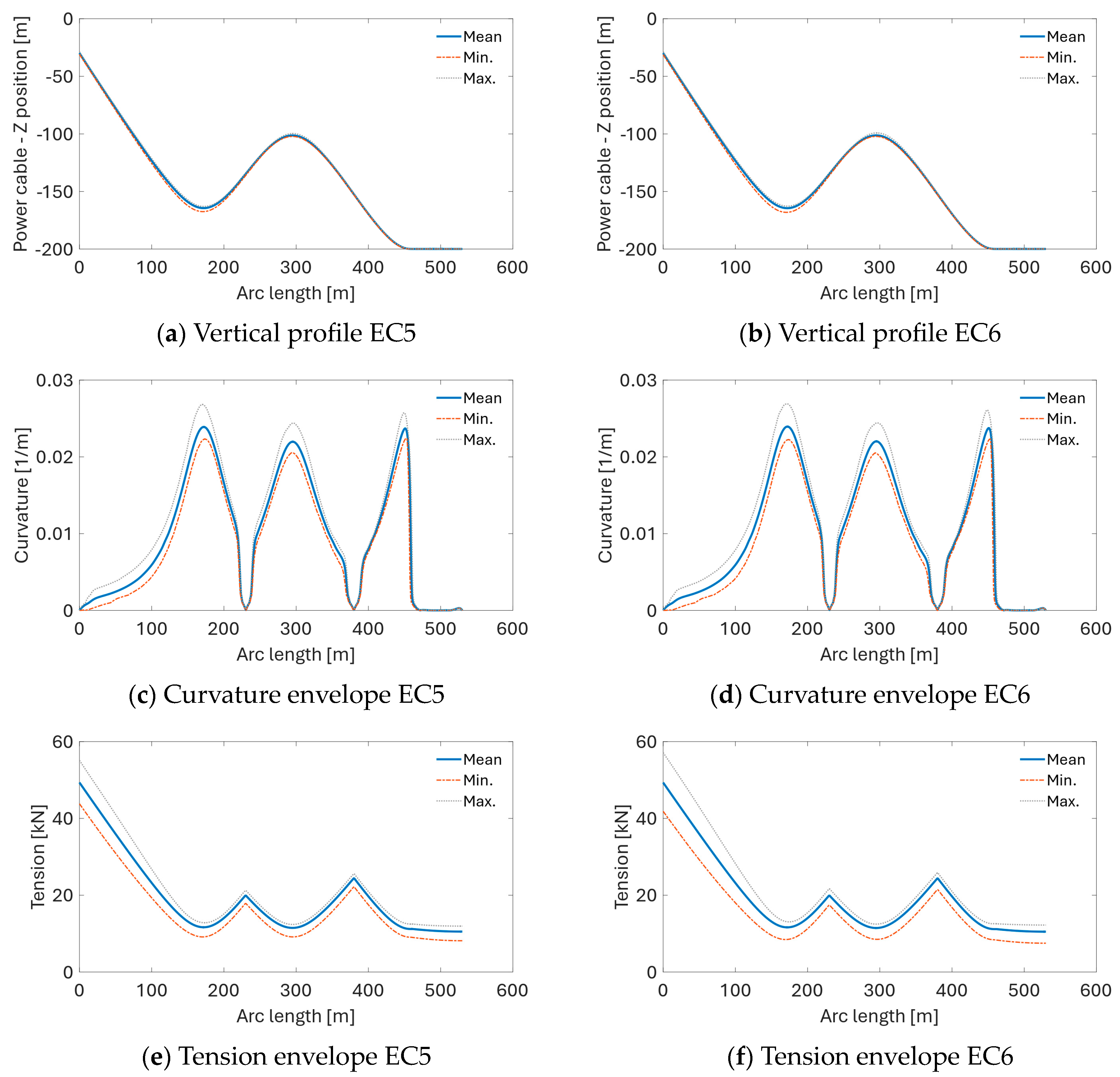
The results from dynamic simulations are presented in Figure 23, Figure 24, Figure 25 and Figure 26. The comparison of maxima and standard deviations of curvature and tension levels experienced by the power cable is presented in Figure 23. The highest curvature is observed under EC3 followed closely by EC2. Under EC2, the cable experiences the largest standard deviation of curvature. Maximum tension levels increase with the ECs of higher wind speeds, significant wave height, and current speed. This trend is also observed for the standard deviation of effective tension experienced by the cable (Figure 23d).
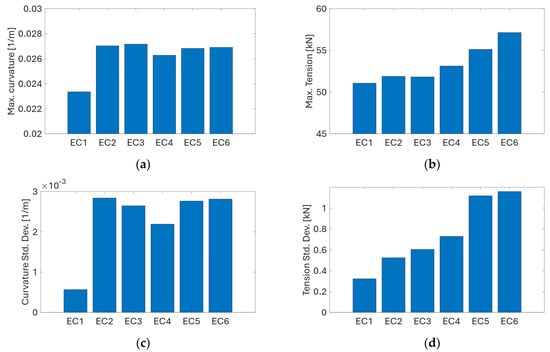
Figure 23.
Comparison of: (a) maximum curvature, (b) maximum tension, (c) curvature standard deviation, (d) tension standard deviation experienced by the power cable under different ECs.
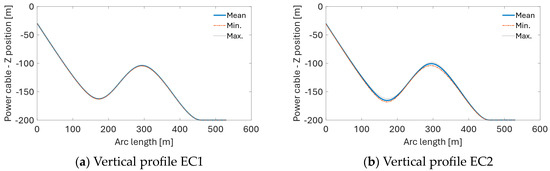
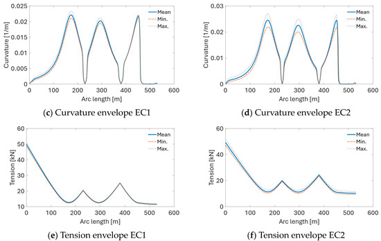
Figure 24.
Envelopes of the cable’s vertical profile, curvature, and effective tension for EC1 and EC2.
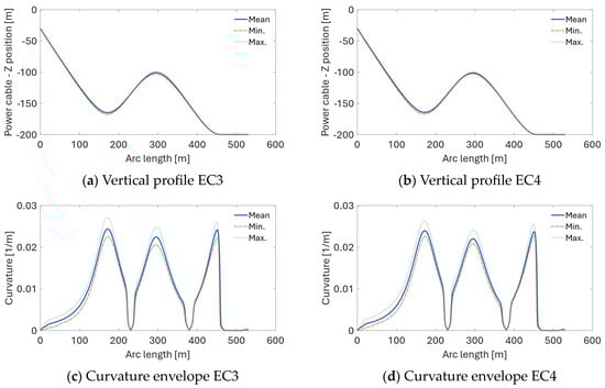
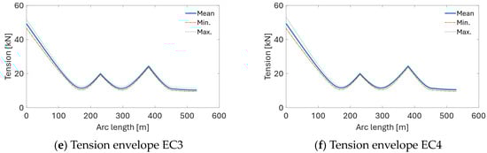
Figure 25.
Envelopes of the cable’s vertical profile, curvature, and effective tension for EC3 and EC4.
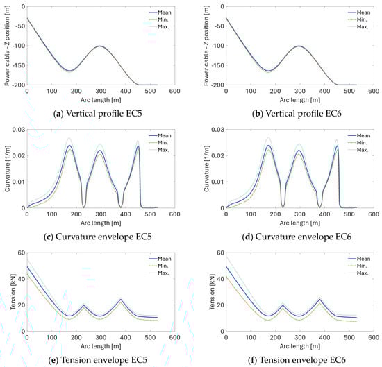
Figure 26.
Envelopes of the cable’s vertical profile, curvature, and effective tension for EC5 and EC6.
3.5. Fatigue Life Estimates
The present fatigue analysis is based on several simplifications and should be interpreted as a concept study of the applicability of the present cable model to a generic FOWT system. During its service life, the dynamic power cable is subject to floater motions as well as wave and current loads, which are sources of fatigue damage, particularly in the case of cyclic bending. Knowledge of site-specific environmental conditions is generally required for accurate fatigue damage estimation. In practice, a long-term joint probability distribution model of wind speed, wave, and current, including directional spreading and seasonality, should be employed. The following analysis presents short-term fatigue damage calculations based on 3 h time series of cyclic stress in the power cable obtained from simulations with different ECs listed in Table 6. The stress time series is derived in OrcaFlex using the stress factor approach, in which the stress is assumed to comprise a tensile contribution (proportional to either wall tension or effective tension) and a bending contribution (proportional to curvature). The stresses used to calculate damage are calculated according to the formula:
where is stress; and are the tension and curvature stress factors, respectively; is the effective tension; and are the components of curvature in the cable’s local x and y directions; and is the circumferential location of the fatigue point. The stress factors (Figure 20) computed using the local UFLEX model of the cable cross-section are used as an input to OrcaFlex. Due to the tensile properties of ETP copper and creep effects, the use of the S-N curve (stress cycle) approach to predict fatigue life has several shortcomings. As pointed out by Karlsen [56], the plastic straining of the conductor has a significant impact on the fatigue life estimation accuracy. Therefore, it is recommended to use the ε-N (strain versus number of cycles to failure) curves in the fatigue analysis of the copper conductors.
Contrary to the traditional S-N curve, the ε-N curve accounts for both elastic and plastic strain. However, due to the limitation of OrcaFlex, which at present supports only the S-N curves for the fatigue analysis, the present fatigue analysis is based on stress cycle counting using the stress factor approach. Figure 27 shows the S-N curves for the steel (DNV [57]) and copper conductor (Nasution [58]) used in the present analysis.
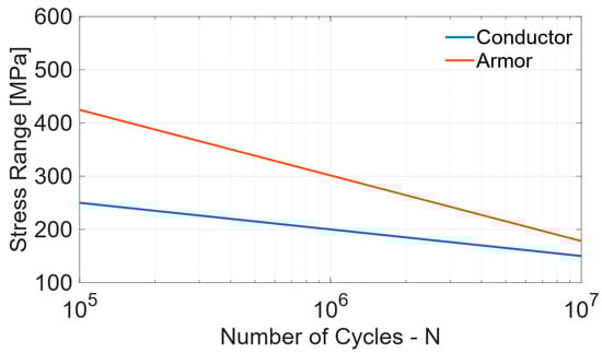
Figure 27.
S-N curves for armor and copper wires.
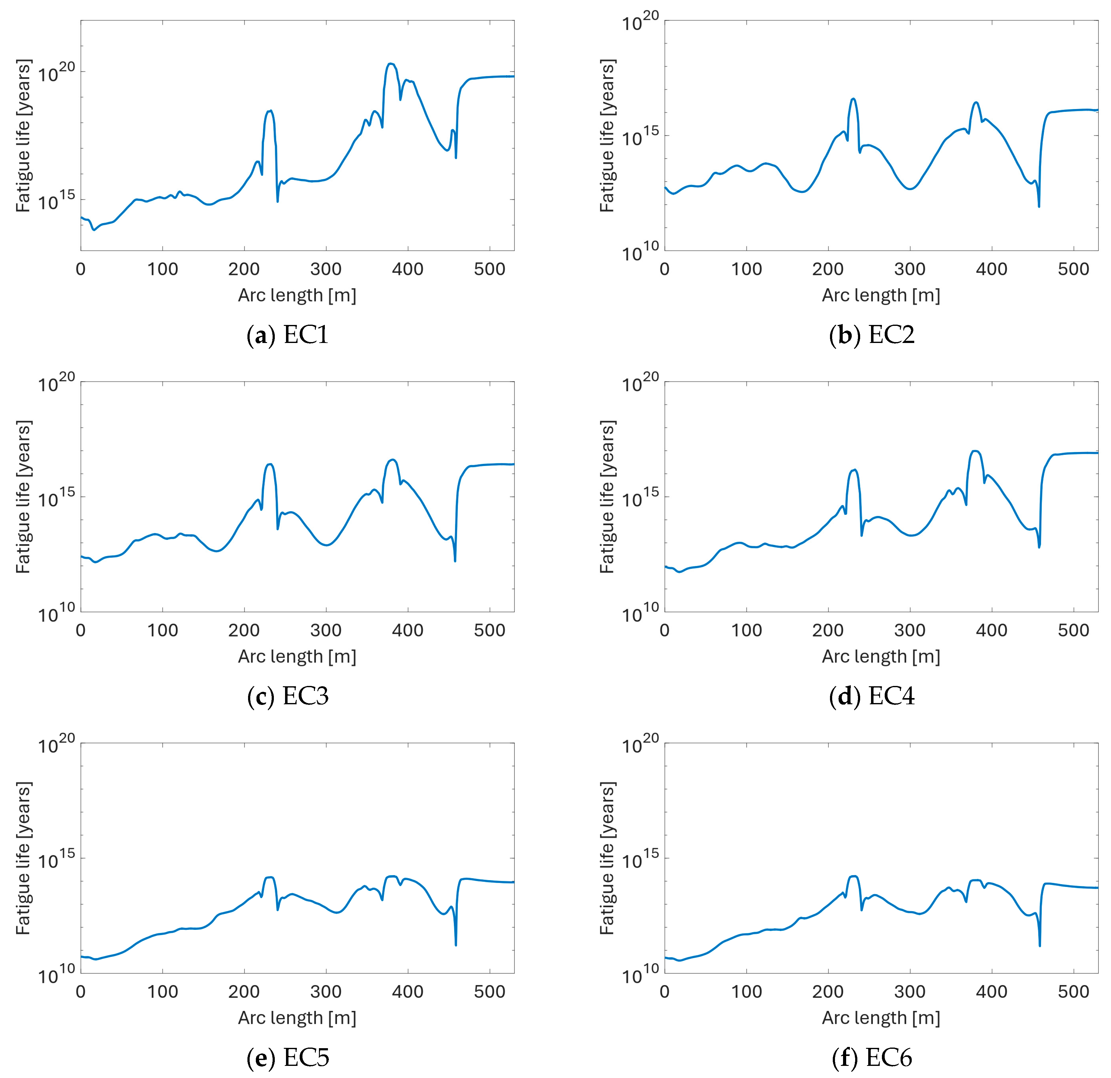
The Rainflow counting method is applied to determine the stress cycles, and the Miner–Palmgren rule is used to calculate the accumulated damage. Figure 28 presents the calculated fatigue life along the cable length. The overall fatigue life is very high due to the relatively small amplitude of cable motions and curvature fluctuations, as presented in the dynamic response analysis part. Another reason is that frictional stress is ignored in the present OrcaFlex stress model. A more advanced algorithm would be required to consider this effect. Nevertheless, there is an observable trend of decreasing fatigue life with increasing wind speed, wave height, and current speed (e.g., from EC1 through EC6).
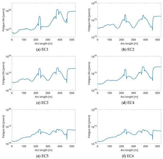
Figure 28.
The predicted fatigue life of the cable under different ECs.
As expected, the locations of minimum fatigue life are at the hang-off point, lazy wave sag bend, hog bend, and touch-down point. In all investigated cases, except for the EC2 case, the most critical location appears at the hang-off point.
4. Conclusions
The present study focuses on proposing three baseline power cable designs for floating offshore wind applications, with an emphasis on addressing the structural requirements that must be met to sustain the dynamic environmental loads experienced over their service life. The presented literature review reinforces the motivation of the study and underlines the need for reference power cable designs suitable for contemporary large-scale floating wind turbines. The study includes a detailed database of structural properties for three reference cable models rated at 33 kV, 66 kV, and 132 kV. Structural properties are obtained from finite element method (FEM) models of respective cable cross-sections built in UFLEX—a special purpose non-linear stress analysis program. Extensive mesh sensitivity studies are performed to ensure the accuracy of predicted structural properties. The cable’s structural design is investigated using global response simulations of an OC3 5MW reference wind turbine coupled with the dynamic power cable in a lazy wave configuration. The models are rigorously validated with a combination of local and global numerical analyses, highlighting the reliability of the designs under dynamic environmental conditions. The analysis results suggest that the dynamic power cable does not significantly affect the response characteristics of the floating wind turbine in the analyzed lazy wave configuration. The feasibility of the present reference cable in floating offshore wind applications is assessed through a simplified analysis of cable fatigue life and structural integrity analysis of the cable in extreme conditions.
Author Contributions
Conceptualization, M.J.J., M.C.O., C.F.L., K.C. and N.Y.; Methodology, M.J.J., M.C.O., C.F.L., K.C. and N.Y.; Software, M.J.J., M.C.O., C.F.L. and N.Y.; Validation, M.J.J., M.C.O., C.F.L., K.C. and N.Y.; Formal analysis, M.J.J., M.C.O., C.F.L., K.C. and N.Y.; Investigation, M.J.J., M.C.O., C.F.L., K.C. and N.Y.; Resources, M.C.O., K.C. and N.Y.; Writing—original draft, M.J.J.; Writing—review & editing, M.J.J., M.C.O., C.F.L., K.C. and N.Y.; Visualization, M.J.J.; Supervision, M.C.O. and N.Y.; Project administration, M.C.O.; Funding acquisition, M.C.O. All authors have read and agreed to the published version of the manuscript.
Funding
The authors acknowledge the support from ImpactWind SouthWest—RCN project number 332034—financed by the Research Council of Norway and the industry partners.
Institutional Review Board Statement
Not applicable.
Informed Consent Statement
Not applicable.
Data Availability Statement
Dataset available on request from the authors.
Acknowledgments
This research work contributes to IEA Task 49 WP2 Reference Power Cable Design. We also thank the anonymous reviewers and the editors for their very helpful comments and suggestions for the manuscript.
Conflicts of Interest
Author Kai Chen was employed by the company Ningbo Orient Wires & Cables Co., Ltd. The remaining authors declare that the research was conducted in the absence of any commercial or financial relationships that could be construed as a potential conflict of interest.
References
- IberBlue Wind, January 2023. Available online: https://www.iberbluewind.com (accessed on 16 January 2023).
- Global Wind Energy Council (GWEC). Floating Offshore Wind—A Global Opportunity. Global Wind Energy Council. Available online: https://gwec.net/wp-content/uploads/2022/03/GWEC-Report-Floating-Offshore-Wind-A-Global-Opportunity.pdf (accessed on 10 November 2023).
- Jonkman, J.M.; Matha, D. Dynamics of offshore floating wind turbines—Analysis of three concepts. Wind Energy 2011, 14, 557–569. [Google Scholar] [CrossRef]
- Cozzi, L.; Wanner, B.; Donovan, C.; Toril, A.; Yu, W. Offshore Wind Outlook 2019: World Energy Outlook Special Report. Available online: https://iea.blob.core.windows.net/assets/495ab264-4ddf-4b68-b9c0-514295ff40a7/Offshore_Wind_Outlook_2019.pdf (accessed on 6 June 2023).
- Worzyk, T. Submarine Power Cables: Design Installation Repair Environmental Aspects; Springer: Dordrecht, Germany, 2009. [Google Scholar]
- Maioli, P. Bending stiffness of submarine cables. In Proceeding of the International Conference on Insulated Power Cables, Versailles, France, 21–25 June 2015. [Google Scholar]
- Love, A.E.H. A Treatise on the Mathematical Theory of Elasticity, 4th ed.; Dover Publications: New York, NY, USA, 1944. [Google Scholar]
- Phillips, J.W.; Costello, G.A. Contact stresses in twisted wire cables. J. Eng. Mech. Div. 1973, 99, 331–341. [Google Scholar] [CrossRef]
- Costello, G.A.; Phillips, J.W. Effective modulus of twisted wire cables. J. Eng. Mech. Div. 1976, 102, 171–181. [Google Scholar] [CrossRef]
- Lutchansky, M. Axial stresses in armor wires of bent submarine cables. J. Eng. Ind. 1969, 91, 687. [Google Scholar] [CrossRef]
- Vinogradov, O.; Atatekin, I.S. Internal friction due to wire twist in bent cable. J. Eng. Mech. 1986, 112, 859–873. [Google Scholar] [CrossRef]
- Hobbs, R.E.; Raoof, M. Interwire slippage and fatigue prediction in stranded cables for TLP tethers. In Behaviour of Offshore Structures; Chryssostomidis, C., Connor, J.J., Eds.; Hemisphere Publishing/McGraw-Hill: New York, NY, USA, 1982; Volume 2, pp. 77–99. [Google Scholar]
- Jolicoeur, C. Comparative study of two semicontinuous models for wire strand analysis. J. Eng. Mech. 1997, 123, 792–799. [Google Scholar] [CrossRef]
- Sævik, S. A finite element model for predicting stresses and slip in flexible pipe armouring tendons at bending gradients. Comput. Struct. 1993, 46, 219–230. [Google Scholar] [CrossRef]
- Sævik, S. A finite element model for predicting longitudinal stresses in non-bonded pipe pressure armours. In Proceedings of the Third European Conference on Flexible Pipes, Umbilicals and Marine Cables, MARINFLEX-99, London, UK, 26–27 May 1999. [Google Scholar]
- Sævik, S. Theoretical and experimental studies of stresses in flexible pipes. Comput. Struct. 2011, 89, 2273–2291. [Google Scholar] [CrossRef]
- Sævik, S.; Ekeberg, K.I. Non-linear stress analysis of complex umbilicals. In Proceedings of the OMAE’2002, Oslo, Norway, 23–28 June 2002. [Google Scholar]
- Sævik, S.; Gray, L.J.; Phan, A. A method for calculating residual and transverse stress effects in flexible pipe pressure spirals. In Proceedings of the OMAE’2001, Rio de Jaineiro, Brazil, 3–8 June 2001. [Google Scholar]
- Sævik, S.; Li, H. Shear interaction and transverse buckling of tensile armours in flexible pipes. In Proceedings of the OMAE’2013, Nantes, France, 9–15 June 2013. [Google Scholar]
- Sævik, S.; Thorsen, M.J. Techniques for predicting tensile armour buckling and fatigue in deep water flexible pipes. In Proceedings of the OMAE’2012, Rio de Jaineiro, Brazil, 1–6 July 2012. [Google Scholar]
- ISO 13628-2; Petroleum and Natural Gas Industries—Design and Operation of Subsea Production Systems—Part 2: Unbonded Flexible Pipe Systems for Subsea and Marine Applications. ISO: Geneva, Switzerland, 2006.
- DNV-OS-F201Offshore Standard: Dynamic Risers, Det Norske Veritas: Oslo, Norway, 2010.
- DNV-OS-501; Offshore Standard: Composite Components. Det Norske Veritas: Oslo, Norway, 2009.
- API 17J; Specifications for Unbonded Flexible Pipe. American Petroleum Institute (API): Washington, DC, USA, 2008; Technical Report.
- Zhang, D.; Ostoja-Starzewski, M. Finite element solutions to the bending stiffness of a single-layered helically wound cable with internal friction. J. Appl. Mech. 2016, 83, 031003. [Google Scholar] [CrossRef]
- Jiang, W.-G. A concise finite element model for pure bending analysis of simple wire strand. Int. J. Mech. Sci. 2012, 54, 69–73. [Google Scholar] [CrossRef]
- Sævik, S.; Bruaseth, S. Theoretical and experimental studies of the axisymmetric behaviour of complex umbilical cross-sections. Appl. Ocean Res. 2005, 27, 97–106. [Google Scholar] [CrossRef]
- Lukassen, T.V.; Gunnarsson, E.; Krenk, S.; Glejbøl, K.; Lyckegaard, A.; Berggreen, C. Tension-bending analysis of flexible pipe by a repeated unit cell finite element model. Mar. Struct. 2019, 64, 401–420. [Google Scholar] [CrossRef]
- Lu, H.; Vaz, M.A.; Caire, M. A finite element model for unbonded flexible pipe under combined axisymmetric and bending loads. Mar. Struct. 2020, 74, 102826. [Google Scholar] [CrossRef]
- Lu, H.; Vaz, M.A.; Caire, M. Alternative analytical and finite element models for unbonded flexible pipes under axisymmetric loads. Ocean Eng. 2021, 225, 108766. [Google Scholar] [CrossRef]
- Fang, P.; Li, X.; Jiang, X.; Hopman, H.; Bai, Y. Bending Study of Submarine Power Cables Based on a Repeated Unit Cell Model. Eng. Struct. 2023, 293, 116606. [Google Scholar] [CrossRef]
- Ménard, F.; Cartraud, P. Solid and 3D beam finite element models for the nonlinear elastic analysis of helical strands within a computational homogenization framework. Comput. Struct. 2021, 257, 106675. [Google Scholar] [CrossRef]
- Ménard, F.; Cartraud, P. A computationally efficient finite element model for the analysis of the non-linear bending behaviour of a dynamic submarine power cable. Mar. Struct. 2023, 91, 103465. [Google Scholar] [CrossRef]
- DNV Helica. Available online: https://www.dnv.com/Publications/helica-69612 (accessed on 1 May 2023).
- SINTEF UFLEX. Available online: https://www.sintef.no/en/software/uflex-stress-analysis-of-power-cables-and-umbilicals/ (accessed on 1 May 2023).
- Sobhaniasl, M.; Petrini, F.; Karimirad, M.; Bontempi, F. Fatigue Life Assessment for Power Cables in Floating Offshore Wind Turbines. Energies 2020, 13, 3096. [Google Scholar] [CrossRef]
- Rentschler, M.U.T.; Adam, F.; Chainho, P. Design optimization of dynamic inter-array cable systems for floating offshore wind turbines. Renew. Sustain. Energy Rev. 2019, 111, 622–635. [Google Scholar] [CrossRef]
- Thies, P.R.; Johanning, L.; Smith, G.H. Assessing mechanical loading regimes and fatigue life of marine power cables in marine energy applications. Proc. Inst. Mech. Eng. Part O J. Risk Reliab. 2011, 226, 18–32. [Google Scholar] [CrossRef]
- Okpokparoro, S.; Sriramula, S. Reliability analysis of floating wind turbine dynamic cables under realistic environmental loads. Ocean Eng. 2023, 278, 114594. [Google Scholar] [CrossRef]
- Martinelli, L.; Lamberti, A.; Ruol, P.; Ricci, P.; Kirrane, P.; Fenton, C.; Johanning, L. Power Umbilical for Ocean Renewable Energy Systems—Feasibility and Dynamic Response Analysis. In Proceedings of the 3rd International Conference on Ocean Energy, Bilbao, Spain, 6–9 October 2010. [Google Scholar]
- Robinson, P. ASM Handbook. Properties of Wrought Coppers and Copper Alloys, Properties and Selection: Nonferrous Alloys and Special-Purpose Materials; ASM International: Almere, The Netherlands, 1990; Volume 2, pp. 265–345. [Google Scholar]
- SINTEF. UFLEX Theory Manual; SINTEF: Trondheim, Norway, 2018. [Google Scholar]
- Ye, N.; Yuan, Z. On Modelling Alternatives of Non-Critical Components in Dynamic Offshore Power Cables. In Proceedings of the 30th International Ocean and Polar Engineering Conference, Virtual, 11–16 October 2020. [Google Scholar]
- Guo, Y.; Ye, N. Numerical and Experimental Study on Full-Scale Test of Typical Offshore Dynamic Power Cable. In Proceedings of the 30th International Ocean and Polar Engineering Conference, Virtual, 11–16 October 2020. [Google Scholar]
- Jonkman, J.; Butterfield, S.; Musial, W.; Scott, G. Definition of a 5-MW Reference Wind Turbine for Offshore System Development; NREL: Golden, CO, USA, 2009; TP-500-38060. [Google Scholar]
- Zhao, S.; Cheng, Y.; Chen, P.; Nie, Y.; Fan, K. A comparison of two dynamic power cable configurations for a floating offshore wind turbine in shallow water. AIP Adv. 2021, 11, 035302. [Google Scholar] [CrossRef]
- Orcina. OrcaFlex ©, Version 11.3. Orcina: Ulverston, UK.
- Schnepf, A.; Pavon, C.L.; Ong, M.C.; Yin, G.; Johnsen, Ø. Feasibility study on suspended inter-array power cables between two spar-type offshore wind turbines. Ocean Eng. 2023, 277, 114215. [Google Scholar] [CrossRef]
- Ahmad, I.B.; Schnepf, A.; Ong, M.C. An Optimisation Methodology for Suspended Inter-Array Power Cable Configurations between Two Floating Offshore Wind Turbines. Ocean Eng. 2023, 278, 114406. [Google Scholar] [CrossRef]
- Johannessen, K.; Meling, T.S.; Haver, S. Joint Distribution for Wind and Waves in the Northern North Sea. Int. J. Offshore Polar Eng. 2002, 12, 19–28. [Google Scholar]
- IEC 61400-3-1:2019; Wind Energy Generation Systems—Part 3-1: Design Requirements for Fixed Offshore Wind Turbines. IEC: Geneva, Switzerland, 2019.
- National Renewable Energy Laboratory (2022). TurbSim. Available online: https://www.nrel.gov/wind/nwtc/turbsim.html (accessed on 14 January 2024).
- DNV-RP-C205; Environmental Conditions and Environmental Loads. Det Norske Veritas: Oslo, Norway, 2019.
- NORSOK N-003; Actions and Action Effects. Standards Norway: Lysaker, Norway, 2017.
- Ramachandran, G.K.V.; Robertson, A.; Jonkman, J.M.; Masciola, M.D. Investigation of Response Amplitude Operators for Floating Offshore Wind Turbines. In Proceedings of the Twenty-third International Offshore and Polar Engineering Conference, Anchorage, AK, USA, 30 June–5 July 2013. [Google Scholar]
- Karlsen, S. Fatigue of copper conductors for dynamic subsea power cables. In Proceedings of the OMAE’2010, Shanghai, China, 6–11 June 2010. [Google Scholar]
- DNV-RP-C203; Fatigue Design of Offshore Steel Structures. Det Norske Veritas: Oslo, Norway, 2021.
- Nasution, F.P.; Sævik, S.; Gjøsteen, J.K.Ø. Finite Element Analysis of the Fatigue Strength of Copper Power Conductors Exposed to Tension and Bending Loads. Int. J. Fatigue 2014, 59, 114–128. [Google Scholar] [CrossRef]


Disclaimer/Publisher’s Note: The statements, opinions and data contained in all publications are solely those of the individual author(s) and contributor(s) and not of MDPI and/or the editor(s). MDPI and/or the editor(s) disclaim responsibility for any injury to people or property resulting from any ideas, methods, instructions or products referred to in the content. |
© 2024 by the authors. Licensee MDPI, Basel, Switzerland. This article is an open access article distributed under the terms and conditions of the Creative Commons Attribution (CC BY) license (https://creativecommons.org/licenses/by/4.0/).