Abstract
Researchers studying urban climates aim to understand phenomena like urban heat islands (UHIs), which describe temperature differences between urban and rural areas. However, studies often lack numerous measurement points and frequently overlook parameters like radiation and air velocity due to the high cost of precision instrumentation. This results in data with a low resolution, particularly in tropical cities where official weather stations are scarce. This research introduces a new, low-tech tool for district-level outdoor thermal comfort assessment and UHI characterization to address these challenges. The automated weather station employs sensors to measure temperature, humidity, wind speed, solar radiation, and globe temperature. The paper details these sensors’ rigorous selection and validation process, followed by a description of the sensor assembly, data acquisition chain, and network operation mechanisms. Calibration outcomes in laboratory and in situ environments highlight the station’s reliability, even in tropical conditions. In conclusion, this weather station offers a cost-effective solution to gathering high-resolution data in urban areas, enabling an improved understanding of the UHI phenomenon and the refinement of urban microclimate numerical models.
1. Introduction
Researchers studying urban climates have been working for a long time to gather environmental data to describe the phenomenon known as an urban heat island (UHI). The temperature difference between urban centers and the rural areas that surround them is referred to as the UHI. In 1833, Howard [1] observed this impact in London and reported a 2 °C temperature difference between the inner city and the suburbs. UHI research has accelerated over the last 20 years and is now a vital component of urban climate change mitigation plans [2]. According to recent research, there are four different types of UHI: the surface heat island at the ground level, the canopy heat island that reaches up to the tallest buildings, the ground heat island that occurs within the soil [3], and the boundary layer heat island that occurs above the buildings and reaches the atmosphere [4,5]. There are two common ways to gather meteorological data on the UHI of the canopy layer: fixed measuring points through weather stations [6] and movable transects employing vehicles [7,8]. The main difficulty lies in balancing cost-effectiveness and spatial and temporal resolution, as each approach has distinct benefits and drawbacks [9]. While permanent weather stations provide long-term data but have limited spatial coverage, mobile transects offer wide spatial coverage but have limited data regularity [10].
Methods for carrying out urban meteorological observations have been developed through extensive research, as described by Oke [11,12,13]. These recommendations state that thermometers and hygrometers should be positioned two to three meters above the ground to reduce interference from cars and people. To prevent airflow turbulence and shading, it is advised to install pyranometers and anemometers above 10 m, respectively [14,15,16].
Researchers from France have conducted studies on UHI in several medium-sized cities worldwide, adhering to these guidelines. These studies encompass a range of measurement methods, including fixed-point measurements in Strasbourg [17,18,19] and mobile transects in Nancy [20]. Although guidance is available for meteorological measurements, temperature and humidity have been the main focus of most urban climate studies [21]. As a result of the high cost of precision instrumentation, these studies frequently provide data with a low spatial or temporal resolution and few measured parameters. They consistently concentrate on temperature and humidity while omitting radiation and air velocity. This restriction is especially severe in tropical cities, where the lack of official weather stations impedes a thorough spatial climate study [22,23]. Thus, to the best of the authors’ knowledge, large, detailed urban microclimate datasets or studies incorporating all parameters impacting thermal comfort are lacking in the literature.
Creating low-tech sensors has come to light as a potential remedy for these problems. Low-tech or suitable technologies meet the criteria for sustainable development and are sustainable, helpful, and easily available. They often involve simple, affordable, energy-efficient, and low-maintenance technologies or methods that satisfy essential requirements [24]. These technologies are especially useful in less developed nations and tropical areas since they make building large networks of weather stations possible on a smaller budget [25,26].
Low-cost and low-power automated weather stations have already been shown to be successful in several applications. For instance, in agriculture, Botero-Valencia et al. created a low-cost climate station for smart agriculture [27,28]. At the same time, Rocha et al. developed an Arduino-based weather station for 155 USD [29]. To monitor solar radiation for photovoltaic fields, Cheddadi et al. developed a station based on an ESP32 microcontroller [30,31]. Similarly, low-cost sensors have been used for energy efficiency in smart buildings [32,33,34,35]. To go beyond the principles of low power and low costs, the low-tech approach was conceptualized in [36]. It refers to a set of methods or technologies based on the fundamental principles of sustainable, frugal, and accessible design [37].
This research presents a new, robust, low-tech tool for district-level outdoor thermal comfort assessment and UHI characterization that is capable of functioning in networks to enhance spatial coverage. Utilizing several sensors, our station can accurately and cost-effectively measure the temperature, relative humidity, wind speed, and solar radiation. Additionally, it incorporates an innovative, low-tech pyranometer and globe temperature measurement, adhering to Vernon’s definition [38]. The gathered high spatial and temporal resolution data are perfect for outdoor comfort and local-scale UHI investigation. The Section 1 of this paper focuses on the rigorous selection and validation process employed for the sensors utilized in the ESP-32 microcontroller-based weather station. This entails meticulous testing procedures to ensure the reliability and accuracy of the chosen sensors. The subsequent section comprehensively describes the sensor assembly, the data acquisition chain, and the network operation mechanisms. This includes detailing the configuration of the sensors, their integration into the weather station, and the protocols established for data transmission and reception. Following this, the Section 3 presents the outcomes of the calibration phases conducted in both laboratory settings and in situ environments. These results are thoroughly analyzed and discussed, particularly concerning the efficacy of the low-tech approach adopted and the overall reliability of the weather station. The article aims to thoroughly explain the sensor selection, assembly, calibration processes, and performance evaluation of the weather station in tropical conditions.
2. Materials and Methods
2.1. General Overview
The main goal of the developed automated weather station is to have UHI characterization performed at the microscale through fixed measurement points. Nevertheless, the concept of the UHI is considered close to the concept of outdoor thermal comfort. In recent studies, the characterization of UHI has been extended beyond more temperature differences to include variations in thermal comfort indices [39]. In [40], the characterization of UHI according to six thermal indicators in 30 megacities of China is reported. Indeed, the UHI effect is more pronounced at night, while the study of outdoor thermal comfort (OTC) is predominantly conducted during daytime. Therefore, various sensors have been implemented into our instrument to afford the investigation of both UHI measurements and OTC. A thermo-hygrometer, selected from several references of digital microcontrollers with temperature and relative humidity measurements, was decided upon for use. A calibrated cup anemometer for performing wind speed measurements was also employed. A low-tech pyranometer for global irradiation was developed for this study. A 40 mm gray globe and a thermocouple measured the globe temperature. These parameters are essential for the computation of thermal comfort indices such as the Universal Thermal Climate Index (UTCI) [41] or the Physiological Equivalent Temperature (PET) [42,43], which can be calculated. Ultimately, the discussion of the outdoor thermal comfort of inhabitants over long periods and the calculation of the UHI intensity within a neighborhood or on a larger scale are possible. Another aim of this study is the collection of several meteorological data in an urban context to facilitate the calibration of numerical models [44]. Indeed, deploying this sensor in the network will contribute to establishing large datasets of urban environmental parameters that are crucial for improving numerical models such as Envi-Met [45] or SOLENE-microclimat [46].
2.2. Validation of the Environmental Sensors
Several low-cost sensors were selected for the measurements of the five parameters. The selection process employed for each parameter is delineated in this part. The aim of optimizing costs and accuracy to create a precise device within a low budget was pursued. The precision objectives stated in the ISO 7726 standard defining the required specifications for measurements in stressful thermal environments were adhered to [47]. A rigorous validation protocol involving two phases, calibration under laboratory conditions and validation in real-world, in situ conditions, was undertaken for each selected sensor. The calibration processes and methods for each type of sensor are described below.
2.2.1. Dry Air Temperature and Humidity
Different studies in the literature, which compared several sensors, were first referred to for choosing the digital thermohygrometer. In [48], the precision of 8 low-cost temperature sensors was assessed by Mobaraki et al., with the results indicating that SHT sensors performed the best. The DHT22 sensor was validated for its performance concerning relative humidity in [49,50].
Based on these previous results, five digital sensors, DHT20, DHT22, SHT31, SHT35, and DS18B20, were selected for testing and calibration under controlled laboratory conditions. These sensors employ a thermistor for air temperature measurements and integrate a capacitive humidity sensor. The detailed specifications for temperature and humidity sensors can be found, respectively, in Table 1 and Table 2. To experiment, at least two units of each sensor were used.

Table 1.
Sensor temperature characteristics according to their datasheet.
Table 2.
Sensor relative humidity characteristics according to their datasheet.
Four type-K thermocouples with an accuracy of 0.1 °C and four Testo 174H devices were utilized for temperature and humidity references. These devices were subjected to regular calibration procedures before being used. The Testo 174H is capable of measuring temperature ranges from −20 to +70 °C with an accuracy of ±0.5 °C, and it includes a capacitive humidity sensor that measures relative humidity with an accuracy of ±3% at 25 °C. A Memmert UF55 oven with a ventilation hatch was used as the climatic chamber to control temperature and humidity. Four scenarios were conducted to assess the performance of the sensors under controlled conditions. Every minute, the relative humidity and temperature were recorded. For each scenario, error indicators such as Mean Absolute Error (MAE), Mean Relative Error (MRE), and Root Mean Square Error (RMSE) were calculated to validate the accuracy of the sensor. These errors were then compared to the tolerances provided in the datasheets of each component. Detailed descriptions of each scenario are given below:
- The first scenario is a step-by-step heating process. The oven temperature was increased by 5 degrees every 60 min from 25 °C to 55 °C. These temperatures were selected to reflect summer temperature conditions and slightly exceed them. At the same time, the relative humidity in the oven varied between 55% and 20%, as presented in Figure 1.
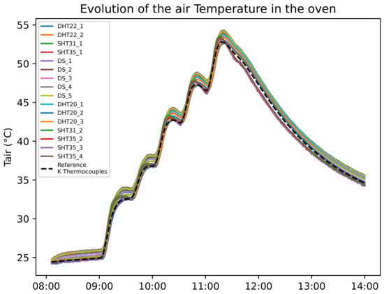
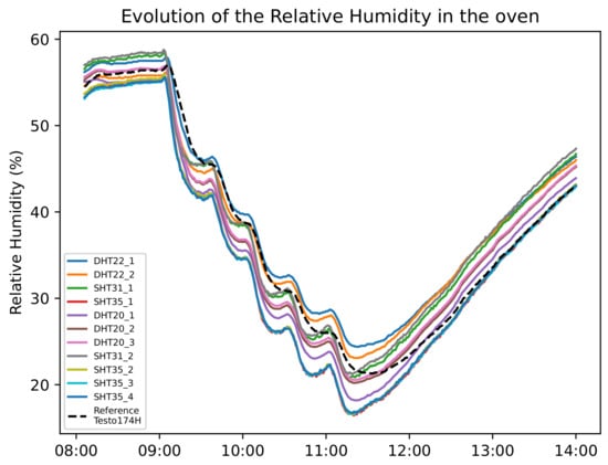 Figure 1. Calibration Scenario 1: Step-by-step heating process for the calibration of the thermo-hygrometer in the oven.
 - The second scenario involved uncontrolled conditions in the oven, with temperature variations between 25 °C and 30 °C and relative humidity from 80% to 50% (ambient conditions), as presented in Figure 2. It should be noted that the oven was turned off, and the variations occurred due to changes in the ambient conditions within the room.
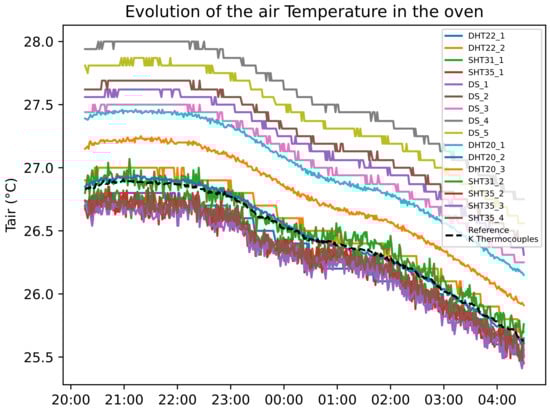
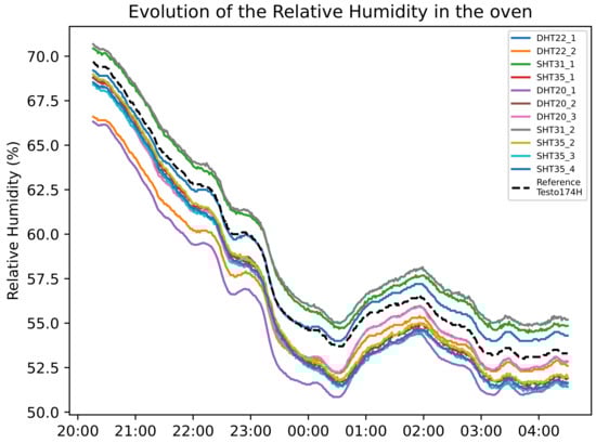 Figure 2. Calibration Scenario 2: Uncontrolled conditions for the calibration of the thermo-hygrometer in the oven.
 - The third scenario involved a rapid temperature increase from 25 °C to 55 °C in the oven. A gradual decrease followed this until it returned to ambient conditions, as presented in Figure 3.
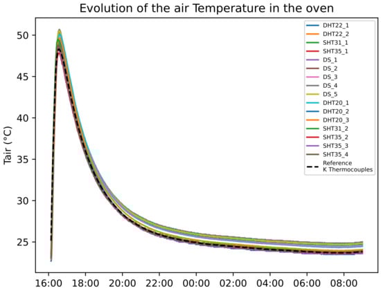
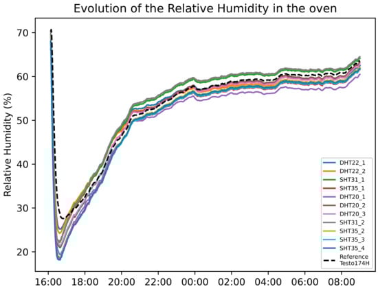 Figure 3. Calibration Scenario 3: Rapid increase in temperature and gradual decrease for the calibration of the thermo-hygrometer in the oven.
 - For the last scenario, all the sensors were left in a room with natural variations for one month.
All the results from the calibration phases for the thermo-hygrometers are discussed and made available in the Section 3.
2.2.2. Mean Radiant Temperature via Globe Temperature
The Mean Radiant Temperature (MRT) is a crucial parameter for calculating thermal comfort indicators, encompassing radiation received from all directions in both short and long wavelengths.
The technique of globe temperature () is frequently employed to evaluate MRT and the Wet BulB Globe Temperature (WBGT) indicator [51]. This technique was first used by Vernon in 1930 [38]; it involves using a matte black globe with a diameter of 15 cm inside of which a temperature sensor is placed. The globe temperature measured in this way takes into account the effects of radiation, convection, and air temperature. The increased use of this technique, attributed to its cost advantage, was reported by Johansson et al. in [52]. Following this, the method for calculating MRT from the globe temperature () is defined by the ISO7726 standard [47]. The calculation incorporates the globe diameter (D) and emissivity (), along with the air velocity () and the air temperature (), as described in the methodology presented below.
Moreover, according to Humphrey [53], a 40 mm globe painted gray better approximates the mean radiant temperature than a standard 15 cm black globe indoors. This statement was also validated in outdoor conditions in [54,55]. Both cited studies undertook a local calibration to determine the relation between the mean radiant temperature and the globe temperature for their subtropical climates. According to these findings, a table tennis ball painted gray and a DS18B20 thermistor were used to obtain the globe temperature in our case.
2.2.3. Wind Measurement
In the literature, three main methods for wind measurement are identified: hot wire or hot ball measurement, ultrasonic sensors, and cup anemometers. Deploying hot wire technology can be challenging, as it does not fare well under outdoor conditions and is susceptible to long-term corrosion. Although ultrasonic technology offers better resilience to outdoor conditions, it comes at a significantly higher cost.
Despite its potential maintenance requirements and limitations in measuring low wind speeds, cup anemometer technology was chosen for our sensor due to its durability under outdoor conditions and its cost-effectiveness.
For our purposes, two types of anemometers were selected based on a cost criterion of around fifty euros: the C2192 [56] and the JL-FS2 cup anemometer [57]. Both are analog devices requiring an input voltage between 9 and 12VDC. The detailed characteristics of these two devices are presented in Table 3.
Table 3.
Sensor wind speed characteristics according to their datasheet.
To validate their usage, the engineering school of the University of Reunion Island, ESIROI, calibrated the two types of anemometers in a wind tunnel. The wind tunnel was equipped with an L Pitot tube monitored via a KIMO C310 multifunction sensor and two ventilators that could reach a wind speed of 10 m/s. The KIMO C310 served as a data acquisition unit for the wind tunnel. The airflow in the tunnel was considered turbulent due to fixed obstacles at the entrance of the duct. The airspeed was set by adjusting the rotation frequency of each ventilator between 15 and 50 Hz. The calibration was undertaken with a gradual increase in air velocity step-by-step from 0.5 m/s to 10 m/s. The air velocity measured using the reference Pitot tube was compared to the one from our anemometer. Each anemometer was calibrated separately because of the limited space in the wind tunnel. Then, the mean relative error was computed compared to the one in the datasheet.
All the calibration results of the anemometer calibration are discussed and made available in Section 3.
2.2.4. Solar Radiation
Challenges are presented in measuring solar radiation with low-cost instruments. The limitations due to the restricted linear response of phototransistors when measuring solar irradiance were demonstrated in [58]. Moreover, the use of low-cost luxometers for measuring solar illuminance and its conversion to irradiance, validated in [59] and based on established conversion relationships from [60,61], faced limitations due to the restricted range and non-linear response of the sensors, limiting further exploration. Nevertheless, a promising, low-cost solution based on a 0.5 W peak photovoltaic cell and an INA219 module for monitoring extreme solar radiation was developed by Chase et al. [62]. This study inspired us to develop a low-tech pyranometer using a photovoltaic cell and a thermistor. The INA219 module is a current shunt and power monitor with an I2C interface, commonly used to monitor power consumption in various applications. The yield of a photovoltaic cell is dependent on the global irradiation (Gh) and the temperature of the cell (Tcell) [63]. This led to the undertaking of a comparison among three calibration models, taking into account these two parameters: the Tcell and the short circuit current of the cell (Isc). A 0.5 Wp silicon monocrystalline solar panel (short-circuit current: = 100 mA; open-circuit voltage: = 5.5 V; Efficiency: 18%; Kingdesun Tech Co., Ltd: Shenzen, China) with a DS18B20 temperature sensor affixed at the back was utilized. It was placed on a horizontal platform adjacent to a pyranometer measuring global irradiation. This setup was used to calibrate our regression model over two months. Four types of models were tested: two simple regression models, one multiple linear regression model, and a random forest model.
First, a simple regression model with only the short circuit current of the cell was tried:
Then another one was applied with only the temperature of the cell:
Then, a multiple linear regression model involving both was applied:
In these equations, a, b, and c represent the coefficients of the linear regression models.
Finally, the random forest model was trained using the RandomForestRegressor function from the sklearn Python library. All the results can be found in Section 3.
2.3. Sensor Design
The designed automated weather station was based on an ESP-32 micro-controller [64]. The main advantage of this chip remains that it includes a Wi-Fi and Bluetooth protocol. It has many digital pins (34) supporting SPI, Serial, and I2C communication protocols. ESP32 is often used in IoT applications, such as in [65,66,67]. It also offers its communication protocol, ESP-NOW, which allows several ESP-32s to communicate together, acting like a network. Linggarjati used ESP-NOW protocol to obtain the temperature from a thermometer with another ESP32, which commanded a hydraulic system. [68] The general diagram representing the sensors and the electronic parts is presented in Figure 4. An ADS1015 (Analog to Digital Converter (ADC)) was added to this chip to improve the analog measurements. Indeed, according to the ESP32 datasheet, the integrated ADC does not support voltages beyond 3.3 V, and its response is not entirely linear, especially at the boundaries of the range (at both the lower and upper ends). An SD card reader was installed to locally store all the collected data. A battery pack of 20,000 mAh at 3.7 V powered with a 6 W solar panel was sized to ensure the autonomy of the entire sensor. Its capacity was designed to operate continuously for up to three consecutive cloudy days with an approximate peak current consumption of 250 mA. The battery level was tracked to detect eventual problems.
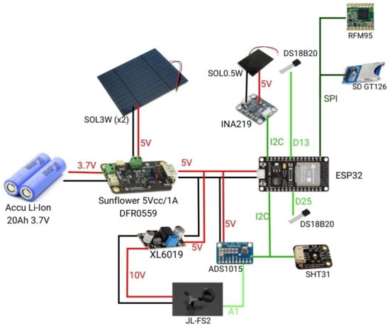
Figure 4.
General diagram of the microcontroller and sensors for the transmitter device.
Assembly and Exterior Design
The assembly of all electronic parts and sensors onto a printed circuit board (PCB) was intended. The authors’ blueprints, bill of materials, Gerber files (which contain detailed information about the layout of the PCB), and pick and place files (which provide precise coordinates for each component) could be accessed. These files were helpful in duplicating the printed circuit. An IP65-rated junction box, specifically designed for outdoor conditions, enclosed the PCB and the battery pack. White-painted square tubing and satellite dish mounting were utilized for the general assembly. The mounting is a cantilever arm, providing distance from the fixing point to mitigate masking effects and related disturbances. This setup allows for the sensor’s placement in various outdoor configurations, including on lamp posts, facades, or trees, with the solar panel’s orientation being adjustable for optimal photovoltaic production. To optimize photovoltaic production at our latitudes, the panel supports were 3D-printed using ASA (Acrylonitrile Styrene Acrylate) plastic at a 20° angle. ASA is a type of plastic frequently utilized in outdoor settings due to its resilience to various weather conditions, notably UV radiation, which is especially crucial in our tropical conditions. However, the use of ASA is not essential and may vary, depending on the context. For instance, wood or other local materials could be used. A solar radiation shield’s necessity to accurately measure the dry air temperature and relative humidity was recognized. The solar radiation shield blocks direct sunlight, which could heat the sensor. The significance of various types of shelters for thermometers to ensure uninterrupted data collection was showcased by Rojas Gregorio et al. [69]. At the same time, a study by Cheung [70] on a low-cost solar radiation shield illustrated its effectiveness in reducing the impact of solar radiation compared to a standard Stevenson screen in temperature measurements. Inspired by these findings, a low-tech solar radiation shield was developed using plastic flower pot saucers connected via threaded rods. A picture of the low-cost, externally mounted station is shown in Figure 5.
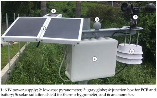
Figure 5.
Photograph of the final assembly of the sensor with all of its components.
2.4. Network and Data Acquisition
The solution was designed to measure micro-scale climatic parameters within a neighborhood as a sensor network distributed across multiple points. The system was designed to function as an 868 MHz LoRa network with two types of nodes: sensors and gateways. They were both based on ESP32. The sensor node was presented in detail in the previous section. Conversely, the gateway, as depicted in Figure 6, is only composed of an SD adapter for data storage and an RFM95 LoRa chip operating at 868 MHz. LoRa 868 is a radio protocol commonly utilized in Europe for IoT applications. It provides communication within a range of up to 200 m in urban or constructed environments and up to several kilometers in open spaces [71].
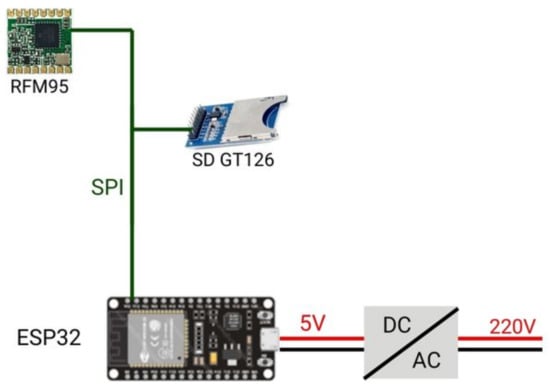
Figure 6.
Conceptual diagram of the gateway device.
Establishing the link between the LoRa sensor network and the database over the internet was facilitated by constructing the gateway. Its primary function was to gather data from various sensors and send it to an online Google Sheet. The Google Sheets solution was chosen for its numerous benefits, including quick implementation, easy accessibility, no-cost availability, intuitive interface, and the ability to access and review the solution any time with an internet connection. The primary purpose of this is to facilitate the live tracking of data. The gateway can establish an internet connection through a Wi-Fi network within a building or via 4G connections. It serves as a slave device, retrieving the date and time from the internet and transmitting this information to the weather station via LoRa every five minutes. The management of up to four weather stations simultaneously is within its capability. Conversely, weather stations collect data from their sensors in various locations and transmit it to their subordinate every ten minutes. When time information is received, their internal real-time clock (RTC) is calibrated if any deviation over time is detected. All the received data are stored in the local memory of the gateway and sent in real time to a Google Sheet using a GoogleAppScript [72]. Serving as the initial layer of the database, the Google Sheet is then interfaced with a Python script, which is used to extract the data and save it in an SQL database. This database is linked to the Grafana software for the display of curves. The general process is depicted in Figure 7.
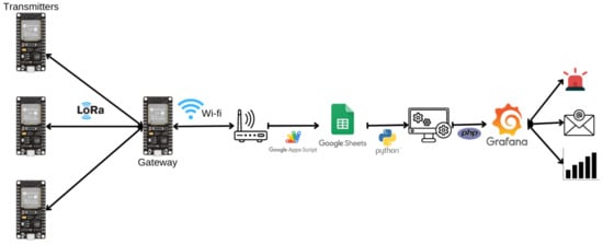
Figure 7.
Diagram of the entire acquisition process from the sensor node to the database.
Security measures and backup routines were developed in the gateway script to minimize the data loss as much as possible. When an internet connection issue arose, all the received data were stored on an SD card via the gateway and sent once the connection was re-established. This process was also applied in cases with an error in the LoRa transmission. Additionally, the gateway checked any missing values within the last three hours, and the sensors were requested to transmit the missing data via LoRa. The general schematic of the C script for the transmitter and gateway is presented in Figure A1 and Figure A2.
2.5. Validation In Situ
The entire operational system underwent testing during an in situ verification phase. The in situ calibration occurred at St Pierre, Reunion Island, between September 2023 and December 2023. The site is located in the western region of the Indian Ocean, namely at a latitude of 21°20’ S and a longitude of 55°29’ E. The region has a tropical climate with high temperatures, averaging around 24°C throughout the year. The humidity is consistently high at 70%, and trade winds prevail for approximately 30% of the year. Our equipment was installed close to the automated weather station located at the PIMENT laboratory within the University of Reunion campus. This weather station is equipped with well-maintained instruments, which include the following:
- Hygrovue 5: Measures air temperature with an accuracy of 0.3 °C and relative humidity within 1.8% (at 25 °C) across the range of 0 to 80% RH and ±3% (at 25 °C) for the range of 80 to 100% RH. The Hygrovue 5 is housed within a 6-plate solar radiation shield.
- A100L2 cup anemometer: Positioned at a height of two meters to measure the air velocity. It boasts an accuracy of 1% + 0.1 m/s within the range of 0.2 m/s to 50 m/s with a start speed of 0.2 m/s.
- CMP11 pyranometer: Measures global horizontal irradiation and offers a directional error of less than 10 W/m² for angles up to 80° relative to the incident solar beam of 1000 W/m² according to its datasheet.
These instruments act as reference sensors to check accuracy in outdoor situations. A gateway was established within the university building to conduct a comprehensive acquisition test at roughly 100 m, as depicted in Figure 8. All the real condition validation results are discussed and made available in the next section.
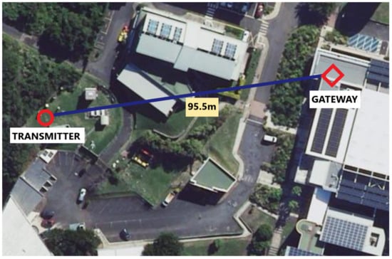
Figure 8.
Aerial perspective of the in situ deployed LoRa devices at St Pierre, La Reunion.
3. Results and Discussion
3.1. Calibration In Vitro
The results of the calibration in laboratory conditions for the thermo-hygrometer and the air velocity in the wind tunnel are presented in this subsection.
3.1.1. Temperature and Humidity
The findings of the three calibration scenarios in the oven are consolidated in Table 4. The average errors obtained nearly correspond to the values specified in the datasheets for each sensor. However, the comprehensive results provided in Figure 9 reveal inconsistencies in the data obtained from various sensors of the same reference. For instance, one DHT20 can exhibit a 0.5 °C discrepancy compared to the other. These results highlight the importance of the calibrating process. The importance of performing extensive calibration before using inexpensive devices is highlighted. Assessing the coherence across sensors and comparing them to a standard allows for the identification and elimination of unreliable sensors. All researchers utilizing inexpensive devices should use this procedure. Validation is essential to obtain precise measurements.
Table 4.
Overall measured accuracy during the calibration process.
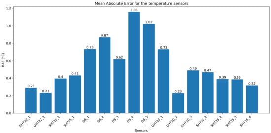
Figure 9.
Comparison of the Mean Absolute Error measured for each temperature sensor in the oven in the Calibration Scenario 1.
Concerning long-term performance, no deviations were observed in the one-month indoor scenario evolution, as shown in Figure 10 and Figure 11. Indeed, the error reported previously remained largely the same after one month for temperature and humidity.
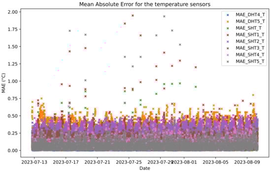
Figure 10.
Tracking over one month of the Mean Absolute Error for the air temperature sensors in laboratory conditions.
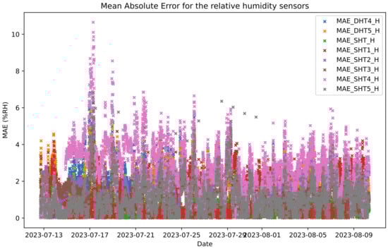
Figure 11.
Tracking over one month of the Mean Absolute Error for the relative humidity sensors in laboratory conditions.
Finally, according to Table 4, the SHT31, SHT35, and DHT22 sensors exhibit the highest accuracy, aligning closely with the specifications outlined in their respective datasheets with an interesting price. The calibration process ensures this low-cost sensor’s validity under the given conditions. The SHT31 was lastly selected for the final choice of sensor. It is sold with an encapsulated design that enhances its durability, providing better resistance to dust and sunlight.
3.1.2. Wind Speed
This subsection presents the results of calibrating the cup anemometer in the wind tunnel. Figure 12 depicts the air velocity (measured in meters per second) obtained by comparing the Pitot reference with the measured analog output voltage of the C2192 anemometer. Calibration was performed by conducting a linear regression analysis between the low-cost sensor’s output voltage (Vout) and the wind speed (Vair) measured using the reference device. The following relationship was derived via linear regression:
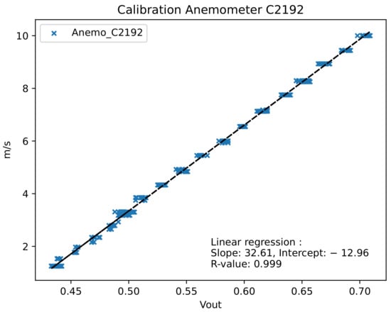
Figure 12.
Linear regression model from output voltage and air velocity obtained to calibrate the C2192 anemometer in the wind tunnel.
Although there is a strong correlation coefficient, it does not align with the model supplied in the product’s datasheet given below:
These findings emphasize the importance of verifying the procedure for low-cost devices. Due to potential unreliability, it is essential to thoroughly calibrate all equipment before utilizing it, as datasheets may need to provide accurate information for this particular type of sensor consistently.
A notable variation was observed after deployment outdoors for two months. Upon reintroducing it to the wind tunnel, a distinct and contrasting pattern emerged after two months of exposure to the elements outdoors. The problem may be related to the sensor’s waterproofing, which is likely affected due to its plastic composition. The C2192 anemometer was subsequently omitted from the study.
In addition, four JL-FS2 anemometers were tested in the wind tunnel. They exhibited better performance when taking into account the specified relationship outlined in the datasheet:
The Relative Error was computed between the Pitot sensor and the measures of air velocity via the low-cost sensor. The values are displayed in Figure 13. We obtained an overall Mean Relative Error of 6.27% for the four anemometers (5.23%, 6.76%, 6.28%, and 6.22%), which was more than the 3% tolerance provided in the datasheet. This additional discrepancy obtained between the low-cost wind sensor readings and the reference can be explained according to their placement in the wind tunnel. Indeed, turbulence at the wind tunnel’s entrance may lead to measurement discrepancies. However, the global absolute error is still acceptable. Thus, the JL-FS2 seems valid for low-cost measurements.
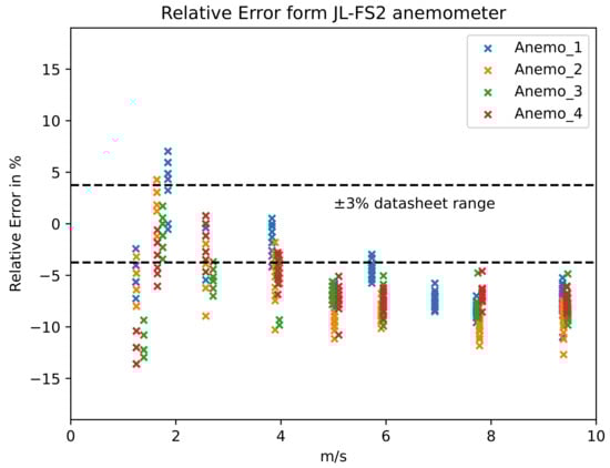
Figure 13.
Relative error obtained with the datasheet model for the windspeed of 4 JL-FS2 Anemometers in the wind tunnel.
The JL-FS2 anemometer was chosen for its more reliable response and durable metal enclosure, which appears more robust than that of C2192.
3.2. Calibration In Situ
This section discusses the validation of the entire sensor and network under in situ conditions. The main objective was to test all sensors in real conditions with outdoor exposure. For this purpose, a 2-month measurement campaign was undertaken. Our low-tech sensor was attached to an official weather station, which is regularly maintained, for validation.
3.2.1. Temperature and Humidity
The functioning of the SHT31 thermo-hygrometer and its homemade ventilated shelter in real conditions was validated by the temperature and relative humidity results. Indeed, the two-month in situ experiments reveal a Mean Absolute Error (MAE) of 0.42 °C, a Mean Relative Error (MRE) of 1.65%, and a Root Mean Square Error (RMSE) of 0.61 °C for the SHT31 temperature measurements. Additionally, an MAE of 2.08%RH, an MRE of 2.8%, and an RMSE of 2.72% were observed for the relative humidity measurements. One week’s results are presented as an example to illustrate the sensor’s trend in Figure 14 and Figure 15. Although the months chosen for calibration took place in the hottest period of the year, the temperature estimation according to the thermometer remained accurate. However, it is noticeable that the radiation shield heated more during peak sun hours compared to the reference weather station. Our solar shield was more exposed to sunlight than the reference in the setup, explaining why the RMSE exceeds 0.5 °C for these points. Similar conclusions can be drawn for relative humidity. As solar radiation increases, the air becomes drier, resulting in the SHT31 measuring slightly lower relative humidity than the reference sensor during the day. Ultimately, the choice of SHT31 sensors with the homemade solar radiation shield was justified for outdoor conditions.
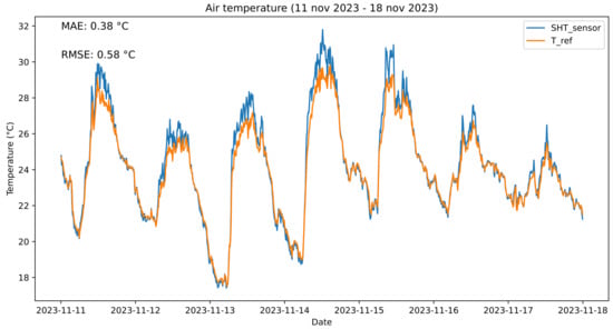
Figure 14.
Comparison of air temperature readings between the low-cost sensor and the reference under real in situ conditions (focusing on one week from 11 November to 18 November 2023).
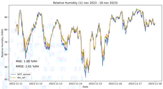
Figure 15.
Comparison of relative humidity readings between the low-cost sensor and the reference under real in situ conditions (focusing on one week from 11 November to 18 November 2023).
3.2.2. Wind Speed in Real Conditions
The average accuracy of the JL-FS2 anemometer was determined based on two months of collected data. Data from one week are provided as an example in Figure 16 to illustrate the general trend observed in the sensors. Outliers in the measurements, attributed to analog voltage readings, are identifiable on this curve. Furthermore, caution is advised when interpreting results for wind values obtained below 0.8 m/s due to the datasheet specifying a start speed range of 0.4 m/s to 0.8 m/s. An error fluctuating around 0.5 m/s was observed. Specifically, the Mean Absolute Error and the Root Mean Square Error were found to be 0.48 m/s and 0.66 m/s, respectively. This discrepancy is partly linked to the slight difference in the positioning of the two sensors, which was not perfectly identical. The placement of the weather mast can influence the airflow and may partially obstruct the airflow, depending on the wind direction. Occasional spikes in the readings were also noted, potentially resulting from the sensors not being synchronized precisely to the second but to the minute. This discrepancy could occur when wind gusts arise within shorter time intervals. Nevertheless, this error level is acceptable, validating the sensor’s performance under actual operating conditions. While the overall trend was consistent across all measurements, this tolerance must be considered when studying thermal comfort and calculating indicators such as the UTCI to interpret the results accurately.
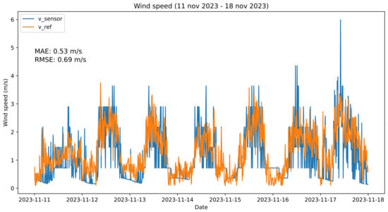
Figure 16.
Comparison of wind speed readings between the low-cost sensor and the reference under real in situ conditions (focusing on one week from 11 November to 18 November 2023).
3.2.3. Global Irradiance
All models’ calibration results are shown in Table 5 below.
Table 5.
Global horizontal irradiance model computed error.
The linear regression models, which incorporate the cell temperature, tend to underestimate the highest radiation values while slightly overestimating the lower ones. This tendency can be attributed to the non-linearity of the cell’s output when it reaches the maximum current values for radiation exceeding 1000 W/m². This behavior is associated with a threshold effect due to PV cell heating, explaining why the regression models incorporating temperature underestimate the extreme values. These models perform better in cloudy conditions than under clear skies, as illustrated in Figure 17. On the other hand, the random forest models provide the best performance in approximating the global horizontal irradiation with the PV cell. The number of estimators was set to 50, 100, and 200 but yielded similar results.
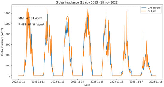
Figure 17.
Comparison of irradiance readings using the multiple linear regression model between the low-cost sensor and the reference under real in situ conditions (focusing on one week from 11 November to 18 November 2023).
3.2.4. Data Quantity Check
The number of missing data was evaluated to validate the LoRa protocol and the acquisition process. The data quantity check formula used is provided below:
The calculation of this ratio for an individual sensor was derived from the anticipated data encompassing the period from 28th November at 12:00 to 9th December at 13:03. The expected number of data lines to be received was 1590. However, only 1579 were obtained. The difference resulted in a data acquisition ratio of 99.31% for the two-week duration. Verification that the data had been securely stored on the SD card of the sensor was obtained, indicating that the problem was limited to the transfer of data over LoRa to the gateway. Although the LoRa communication protocol has been confirmed for operation within this distance, obtaining comprehensive datasets may require including data from the local memory of each sensor. While real-time transmission offers advantages for fast data monitoring, more is needed to gather comprehensive datasets.
3.3. The Low-Tech Approach
The network of weather stations was established following the low-tech approach described in [36]. It relies on fundamental principles, which can be grouped into three types: technological, social, and organizational [37]. The designed sensor adheres to the principle of frugality through the optimal sizing of each piece of equipment to address the need to obtain accurate data for microclimate and thermal comfort evaluation. This study highlights that low-tech solutions can be sufficient to achieve high-accuracy measurements. Low-tech devices can undergo calibration, utilizing high-tech methods such as machine learning algorithms like random forest or high-precision materials, validating them for widespread replication and utilization. This enables technological optimization by solely using appropriate technology to fulfill a specific need. In this case, the design aims to meet the requirements outlined in the ISO7726 standard, as presented in Table 6. The designed sensor has a few areas for improvement compared to ISO7726 for wind and radiation measurements. Thus, this implies that the calculated OTC values will have a more significant uncertainty than that prescribed in the standard but will still reasonably reflect reality. Most importantly, the sensor can precisely characterize UHI in terms of temperature difference and humidity or thermal comfort indicators that involve both, such as the heat index established by Steadman [73].
Table 6.
Table of uncertainties for the sensors obtained from the calibration data.
The device is robust, enduring year-round UV, rain, and wind conditions. Additionally, it has been designed for easy repairability, allowing each part to be replaced without affecting the overall functioning. A regular maintenance routine could enhance the durability and reliability of its measurements. The main challenge is to keep the solar panels clean from dust, maximizing their efficiency. Cleaning of the solar panels should be done approximately every two weeks, depending on the frequency of precipitation that may naturally wash them. For the anemometer, a simple visual inspection every month can be advised to detect any potential sticking due to dust accumulation. If necessary, the anemometer should be regularly freed up. Additionally, an annual detailed check of every sensor of the station is advised to ensure proper operation and calibration.
There is also a focus on power consumption, aiming for maximum efficiency using LoRa and sustainably sourcing power from renewable solar sources. In complement to these principles, accessibility remains a crucial challenge for this technology, which can be addressed through cost-effectiveness and open access to scripts and blueprints, fostering cooperation and continuous improvement. The cost for one device is estimated in Table 7 at 193 EUR in December 2023. Affordable costs will enable the deployment of this technology in regions facing economic constraints, facilitating the study of urban heat islands and thermal comfort in tropical zones. In wealthier regions, it will allow for the proliferation of stations and the development of extensive sensor networks, enabling more precise microclimate studies and better calibration of numerical models. The station was designed to be constructed anywhere in the world, especially in tropical environments. It perfectly fulfills this need. In other contexts, adaptations can be made to better suit specific conditions. For example, slight modifications to materials may be necessary; for instance, in colder conditions, the resistance to freezing has not been tested. Additionally, it is possible to order all of these sensors online on major purchasing platforms. This type of sensor is growing in popularity and becoming more accessible, making it easy to order. Its validation through this paper will help spread its use among researchers worldwide. All the characteristics of the designed device are summarized in Table 8.
Table 7.
Bill of materials and costs assessed in December 2023 (excluding taxes).
Table 8.
Summary of the characteristics of the designed weather station.
4. Conclusions
The study presented in this article highlights the effectiveness and accessibility of an automated weather station designed with a low-tech approach to characterize urban heat islands (UHIs) and assess outdoor thermal comfort in urban areas. The station, which conducts microclimatic measurements, demonstrates that even with an economical design, the accuracy and reliability of the collected data are not compromised, validating its effectiveness in demanding tropical conditions, such as those encountered on Reunion Island.
The practical importance of this research is significant for urban planners, environmental policymakers, and the scientific community, offering an economical and reproducible method for collecting critical environmental data. This is essential for adapting cities to climate change and improving the urban quality of life. Moreover, this weather station solution presents several advantages for them. Firstly, its cost-effectiveness provides a budget-friendly option for acquiring quality equipment, allowing resources to be allocated to other essential projects. Secondly, its modular design offers flexibility, enabling customization to suit specific needs and environments. Lastly, by using this technology, planners and policymakers can gain better insights into environmental challenges, empowering them to make informed decisions and develop more effective strategies for urban adaptation and mitigation. However, it is acknowledged that the study faced limitations, particularly in terms of its geographical scope and local climatic variations. Future research could see this approach expanded to other regions by integrating additional sensors and applying more advanced data analysis techniques to understand UHI dynamics comprehensively. For instance, the station’s resistance to freezing has not been tested in colder conditions, and the validation of sensors in subzero air temperature conditions has not been performed. Designed to be cost-effective and easy to maintain, deploy, and operate within a network, this device was proven reliable in tropical conditions, paving the way to generating valuable high-resolution datasets in urban areas. Future exploration of these data will lead to a better understanding of the UHI phenomenon at various scales within cities, refining the numerical models of an urban microclimate.
The future of our approach relies on international collaboration, inviting researchers and practitioners to adopt, adapt, and improve this weather station. This will contribute to a global database on urban microclimates, enriching our understanding of UHIs and fostering the development of innovative solutions for contemporary urban challenges, particularly in the worldwide context of climate change evolution.
Author Contributions
A.L.: conceptualization, investigation, data curation, methodology, writing—original draft, and visualization. B.M.-D.: conceptualization and writing—review and editing. H.B.: writing—review and editing. G.R.: conceptualization, methodology, writing—review and editing, validation, and project administration. All authors have read and agreed to the published version of the manuscript.
Funding
This research was conducted as part of the ICUTROPIC project, funded by Action Logement Services Group’s Overseas Innovation Plan under contract number 1070524-DROM. It was also carried out in partnership with SHLMR.
Informed Consent Statement
Not applicable.
Data Availability Statement
The components needed to replicate the sensor can be supplied upon request.
Acknowledgments
We sincerely thank Action Logement Services and SHLMR for their trust. We would also like to express our gratitude the University of La Reunion and the PIMENT laboratory for their technical and administrative support.
Conflicts of Interest
The authors declare no conflicts of interest.
Abbreviations
The following abbreviations are used in this manuscript:
| MAE | Mean Absolute Error |
| MRE | Mean Relative Error |
| MRT | Mean radiant temperature |
| OTC | Outdoor thermal comfort |
| PCB | Printed Circuit Board |
| PET | Physiological Equivalent Temperature |
| PV | Photovoltaic |
| RMSE | Root Mean Square Error |
| UHI | Urban heat island |
| UTCI | Universal Thermal Climate Index |
Appendix A. Diagram of the C Code
Appendix A.1. Diagram of Transmitter Code

Figure A1.
Diagram of Transmitter device’s code synoptic.
Figure A1.
Diagram of Transmitter device’s code synoptic.

Appendix A.2. Diagram of Gateway Code

Figure A2.
Diagram of Gateway device’s code synoptic.
Figure A2.
Diagram of Gateway device’s code synoptic.

References
- Howard, L. The Climate of London; AUC: Tokyo, Japan, 1833. [Google Scholar]
- Pelling, M.; Prakash, A.; Zheng, Y.; Ziervogel, G.; Cartwright, A.; Dhar, T.; Evans, B.; Hadi, S.P.; Handayani, W.; Hondula, D.; et al. 2022: Cities, Settlements and Key Infrastructure. In Climate Change 2022: Impacts, Adaptation and Vulnerability; Contribution of Working Group II to the Sixth Assessment Report of the Intergovernmental Panel on Climate Change; Cambridge Press: Cambridge, UK, 2022. [Google Scholar]
- Worsa-Kozak, M.; Arsen, A. Groundwater Urban Heat Island in Wrocław, Poland. Land 2023, 12, 658. [Google Scholar] [CrossRef]
- Oke, T.R. Boundary Layer Climates, 2nd ed.; Routledge: London, UK, 2009; OCLC: 51200739. [Google Scholar]
- Kim, S.W.; Brown, R.D. Urban heat island (UHI) intensity and magnitude estimations: A systematic literature review. Sci. Total. Environ. 2021, 779, 146389. [Google Scholar] [CrossRef] [PubMed]
- Tso, C. A survey of urban heat island studies in two tropical cities. Atmos. Environ. 1996, 30, 507–519. [Google Scholar] [CrossRef]
- Huang, J.M.; Chang, H.Y.; Wang, Y.S. Spatiotemporal Changes in the Built Environment Characteristics and Urban Heat Island Effect in a Medium-Sized City, Chiayi City, Taiwan. Sustainability 2020, 12, 365. [Google Scholar] [CrossRef]
- Huang, J.M.; Chang, H.Y.; Chen, L.C.; Wang, Y.S. Canopy-scale Built-environment Characteristics and Urban Heat Island Effect in a Tropical Medium-sized City. Sustainability 2021, 13, 868. [Google Scholar] [CrossRef]
- Charabi, Y.; Bakhit, A. Assessment of the canopy urban heat island of a coastal arid tropical city: The case of Muscat, Oman. Atmos. Res. 2011, 101, 215–227. [Google Scholar] [CrossRef]
- Romero Rodríguez, L.; Sánchez Ramos, J.; Álvarez Domínguez, S. Simplifying the process to perform air temperature and UHI measurements at large scales: Design of a new APP and low-cost Arduino device. Sustain. Cities Soc. 2023, 95, 104614. [Google Scholar] [CrossRef]
- Oke, T.R. Initial Guidance to Obtain Representative Meteorogical Data; World Meteorological Organization: Geneva, Switzerland, 2004; Volume 81. [Google Scholar]
- Oke, T.R. Towards better scientific communication in urban climate. Theor. Appl. Climatol. 2006, 84, 179–190. [Google Scholar] [CrossRef]
- Liu, Z.; Cheng, K.Y.; He, Y.; Jim, C.; Brown, R.D.; Shi, Y.; Lau, K.; Ng, E. Microclimatic measurements in tropical cities: Systematic review and proposed guidelines. Build. Environ. 2022, 222, 109411. [Google Scholar] [CrossRef]
- Vesala, T.; Kljun, N.; Rannik, Ü.; Rinne, J.; Sogachev, A.; Markkanen, T.; Sabelfeld, K.; Foken, T.; Leclerc, M.Y. Flux and concentration footprint modelling. Model. Pollut. Complex Environ. Syst. 2010, 2, 339–355. [Google Scholar]
- Kljun, N.; Rotach, M.; Schmid, H. A Three-Dimensional Backward Lagrangian Footprint Model For A Wide Range Of Boundary-Layer Stratifications. Bound.-Layer Meteorol. 2002, 103, 205–226. [Google Scholar] [CrossRef]
- Kljun, N.; Calanca, P.; Rotach, M.W.; Schmid, H.P. A Simple Parameterisation for Flux Footprint Predictions. Bound.-Layer Meteorol. 2004, 112, 503–523. [Google Scholar] [CrossRef]
- Fischer, L. Phénomènes radiatifs et îlot de chaleur urbain dans l’agglomération de Strasbourg. RGE 2005, 45, 99–112. [Google Scholar] [CrossRef]
- Hassani, N.; Drogue, G. Mesure et spatialisation de l’îlot de chaleur urbain dans l’aire urbaine de Metz Métropole: Premiers résultats de la campagne de mesure 2019. Climatologie 2020, 17, 8. [Google Scholar] [CrossRef]
- Foissard, X. L’îlot de Chaleur Urbain et le Changement Climatique: Application à l’Agglomération Rennaise; Géographie, Université Rennes 2: Rennes, France, 2015. [Google Scholar]
- Leconte, F. Caractérisation des Îlots de Chaleur Urbain Par Zonage Climatique et Mesures Mobiles: Cas de Nancy, Climatologie; Université de Lorraine: Metz, France, 2015. [Google Scholar]
- Sun, C.Y.; Kato, S.; Gou, Z. Application of Low-Cost Sensors for Urban Heat Island Assessment: A Case Study in Taiwan. Sustainability 2019, 11, 2759. [Google Scholar] [CrossRef]
- Giridharan, R.; Emmanuel, R. The impact of urban compactness, comfort strategies and energy consumption on tropical urban heat island intensity: A review. Sustain. Cities Soc. 2018, 40, 677–687. [Google Scholar] [CrossRef]
- Sari, D.P. A Review of How Building Mitigates the Urban Heat Island in Indonesia and Tropical Cities. Earth 2021, 2, 653–666. [Google Scholar] [CrossRef]
- Khalil, H.A.E.E.; Ibrahim, A.; Elgendy, N.; Makhlouf, N. Enhancing Livability in Informal Areas: A Participatory Approach to Improve Urban Microclimate in Outdoor Spaces. Sustainability 2022, 14, 6395. [Google Scholar] [CrossRef]
- Nsabagwa, M.; Byamukama, M.; Kondela, E.; Otim, J.S. Towards a robust and affordable Automatic Weather Station. Dev. Eng. 2019, 4, 100040. [Google Scholar] [CrossRef]
- Sudantha, B.H.; Warusavitharana, E.J.; Ratnayake, R.; Mahanama, P.K.; Cannata, M.; Strigaro, D. Appropriateness of low cost sensor network for environmental monitoring in a tropical country: Experience and lessons learnt from real world deployment. PeerJ PrePrints 2018, 6, e27224v1. [Google Scholar] [CrossRef][Green Version]
- Botero-Valencia, J.S.; Mejia-Herrera, M.; Pearce, J.M. Low cost climate station for smart agriculture applications with photovoltaic energy and wireless communication. HardwareX 2022, 11, e00296. [Google Scholar] [CrossRef]
- Abdelmoneim, A.A.; Khadra, R.; Elkamouh, A.; Derardja, B.; Dragonetti, G. Towards Affordable Precision Irrigation: An Experimental Comparison of Weather-Based and Soil Water Potential-Based Irrigation Using Low-Cost IoT-Tensiometers on Drip Irrigated Lettuce. Sustainability 2024, 16, 306. [Google Scholar] [CrossRef]
- Rocha, J.V.; Magalhães, R.R.; Carvalho, L.G.d.; Diotto, A.V.; Barbosa, B.H.G. Development of a low-cost weather station and real-time monitoring for automated irrigation management. Acta Scientiarum Technol. 2022, 44, e59244. [Google Scholar] [CrossRef]
- Cheddadi, Y.; Cheddadi, H.; Cheddadi, F.; Errahimi, F.; Es-sbai, N. Design and implementation of an intelligent low-cost IoT solution for energy monitoring of photovoltaic stations. SN Appl. Sci. 2020, 2, 1165. [Google Scholar] [CrossRef]
- Morón, C.; Diaz, J.P.; Ferrández, D.; Saiz, P. Design, Development and Implementation of a Weather Station Prototype for Renewable Energy Systems. Energies 2018, 11, 2234. [Google Scholar] [CrossRef]
- Cano-Suñén, E.; Martínez, I.; Fernández, Á.; Zalba, B.; Casas, R. Internet of Things (IoT) in Buildings: A Learning Factory. Sustainability 2023, 15, 12219. [Google Scholar] [CrossRef]
- Mobaraki, B.; Lozano-Galant, F.; Soriano, R.; Castilla Pascual, F. Application of Low-Cost Sensors for Building Monitoring: A Systematic Literature Review. Buildings 2021, 11, 336. [Google Scholar] [CrossRef]
- Martín-Garín, A.; Millán-García, J.; Baïri, A.; Millán-Medel, J.; Sala-Lizarraga, J. Environmental monitoring system based on an Open Source Platform and the Internet of Things for a building energy retrofit. Autom. Constr. 2018, 87, 201–214. [Google Scholar] [CrossRef]
- Malet-Damour, B.; Guichard, S.; Jean, A.P.; Miranville, F.; Boyer, H. SHADECO: A low-cost shadow-ring for diffuse measures: State of the art, principles, design and application. Renew. Energy 2018, 117, 71–84. [Google Scholar] [CrossRef]
- Tanguy, A.; Carrière, L.; Laforest, V. Low-tech approaches for sustainability: Key principles from the literature and practice. Sustain. Sci. Pract. Policy 2023, 19, 2170143. [Google Scholar] [CrossRef]
- Guimbretiere, G.; Hodencq, S.; Balland, M. Une Approche de la Low-Tech Dans l’Enseignement Supérieur et la Recherche. La Pensée Écologique. 2022. Available online: https://hal.science/hal-03585151v2 (accessed on 20 February 2024).
- Vernon, H. The measurement of radiant heat in relation to human comfort. J. Ind. Hyg. 1932, 14, 95–111. [Google Scholar]
- Ho, H.C.; Knudby, A.; Xu, Y.; Hodul, M.; Aminipouri, M. A comparison of urban heat islands mapped using skin temperature, air temperature, and apparent temperature (Humidex), for the greater Vancouver area. Sci. Total. Environ. 2016, 544, 929–938. [Google Scholar] [CrossRef]
- Wang, C.; Zhan, W.; Li, L.; Wang, S.; Wang, C.; Miao, S.; Du, H.; Jiang, L.; Jiang, S. Urban heat islands characterized by six thermal indicators. Build. Environ. 2023, 244, 110820. [Google Scholar] [CrossRef]
- Jendritzky, G.; de Dear, R.; Havenith, G. UTCI-Why another thermal index? Int. J. Biometeorol. 2011, 56, 421–428. [Google Scholar] [CrossRef]
- Höppe, P. The physiological equivalent temperature – a universal index for the biometeorological assessment of the thermal environment. Int. J. Biometeorol. 1999, 43, 71–75. [Google Scholar] [CrossRef]
- Walther, E.; Goestchel, Q. The P.E.T. comfort index: Questioning the model. Build. Environ. 2018, 137, 1–10. [Google Scholar] [CrossRef]
- Sayad, B.; Helmi, M.R.; Osra, O.A.; Abed, A.M.; Alhubashi, H.H. Microscale Investigation of Urban Heat Island (UHI) in Annaba City: Unveiling Factors and Mitigation Strategies. Sustainability 2024, 16, 747. [Google Scholar] [CrossRef]
- Bruse, M.; Fleer, H. Simulating surface–plant–air interactions inside urban environments with a three dimensional numerical model. Environ. Model. Softw. 1998, 13, 373–384. [Google Scholar] [CrossRef]
- Musy, M.; Malys, L.; Morille, B.; Inard, C. The use of SOLENE-microclimat model to assess adaptation strategies at the district scale. Urban Clim. 2015, 14, 213–223. [Google Scholar] [CrossRef]
- ISO7726, A; Ergonomics of the Thermal Environment—Instruments for Measuring Physical Quantities. ISO: Geneva, Switzerland, 2002.
- Mobaraki, B.; Komarizadehasl, S.; Castilla Pascual, F.J.; Lozano-Galant, J.A. Application of Low-Cost Sensors for Accurate Ambient Temperature Monitoring. Buildings 2022, 12, 1411. [Google Scholar] [CrossRef]
- Mobaraki, B.; Komarizadehasl, S.; Pascual, F.J.C.; Antonio, J.; Galant, L. Determination of environmental parameters based on Arduino based low-cost sensors. In Proceedings of the RTCEE International Conference, Virtual, 10–12 November 2020. [Google Scholar]
- Salamone, F.; Belussi, L.; Danza, L.; Ghellere, M.; Meroni, I. Design and Development of nEMoS, an All-in-One, Low-Cost, Web-Connected and 3D-Printed Device for Environmental Analysis. Sensors 2015, 15, 13012–13027. [Google Scholar] [CrossRef]
- Budd, G.M. Wet-bulb globe temperature (WBGT)—Its history and its limitations. J. Sci. Med. Sport 2008, 11, 20–32. [Google Scholar] [CrossRef]
- Johansson, E.; Thorsson, S.; Emmanuel, R.; Krüger, E. Instruments and methods in outdoor thermal comfort studies—The need for standardization. Urban Clim. 2014, 10, 346–366. [Google Scholar] [CrossRef]
- Humphreys, M. The optimum diameter for a globe thermometer for use indoors. Ann. Occup. Hyg. 1977, 20, 135–140. [Google Scholar] [CrossRef] [PubMed]
- Ouyang, W.; Liu, Z.; Lau, K.; Shi, Y.; Ng, E. Comparing different recalibrated methods for estimating mean radiant temperature in outdoor environment. Build. Environ. 2022, 216, 109004. [Google Scholar] [CrossRef]
- Banfi, A.; Tatti, A.; Ferrando, M.; Fustinoni, D.; Zanghirella, F.; Causone, F. An experimental technique based on globe thermometers for the measurement of mean radiant temperature in urban settings. Build. Environ. 2022, 222, 109373. [Google Scholar] [CrossRef]
- Adafruit. C2192 Anemometer Datasheet. Available online: https://cdn-shop.adafruit.com/product-files/1733/C2192_datasheet.pdf (accessed on 15 December 2023).
- DFRobot. JL-FS2 Anemometer Datasheet. Available online: https://wiki.dfrobot.com/Wind_Speed_Sensor_Voltage_Type_0-5V__SKU_SEN0170 (accessed on 15 December 2023).
- Tohsing, K.; Phaisathit, D.; Pattarapanitchai, S.; Masiri, I.; Buntoung, S.; Aumporn, O.; Wattan, R. A development of a low-cost pyranometer for measuring broadband solar radiation. J. Phys. Conf. Ser. 2019, 1380, 012045. [Google Scholar] [CrossRef]
- Lorenzo, O.G.; Suárez-García, A.; Peña, D.G.; Fuente, M.G.; Granados-López, D. A Low-Cost Luxometer Benchmark for Solar Illuminance Measurement System Based on the Internet of Things. Sensors 2022, 22, 7107. [Google Scholar] [CrossRef] [PubMed]
- Michael, P.R.; Johnston, D.E.; Moreno, W. A conversion guide: Solar irradiance and lux illuminance. J. Meas. Eng. 2020, 8, 153–166. [Google Scholar] [CrossRef]
- Fakra, A.; Boyer, H.; Miranville, F.; Bigot, D. A simple evaluation of global and diffuse luminous efficacy for all sky conditions in tropical and humid climate. Renew. Energy 2011, 36, 298–306. [Google Scholar] [CrossRef]
- Chase, O.A.; Teles, M.B.; de Jesus dos Santos Rodrigues, M.; de Almeida, J.F.S.; Macêdo, W.N.; da Costa Junior, C.T. A Low-Cost, Stand-Alone Sensory Platform for Monitoring Extreme Solar Overirradiance Events. Sensors 2018, 18, 2685. [Google Scholar] [CrossRef]
- Saloux, E.; Teyssedou, A.; Sorin, M. Explicit model of photovoltaic panels to determine voltages and currents at the maximum power point. Sol. Energy 2011, 85, 713–722. [Google Scholar] [CrossRef]
- Espressif. Esp32 Datasheet. Available online: https://www.espressif.com/sites/default/files/documentation/esp32_datasheet_en.pdf (accessed on 6 October 2023).
- Peña, G.; Alberto, J. Cost Effective Technology Applied to Domotics and Smart Home Energy Management Systems; Accepted: 2022-02-17T12:19:58Z; Universidad de Córdoba: Cordoba, Colombia, 2022. [Google Scholar]
- Hermansyah; Kasim; Yusri, I.K. Solar Panel Remote Monitoring and Control System on Miniature Weather Stations Based on Web Server and ESP32. Int. J. Recent Technol. Appl. Sci. 2020, 2, 1–24. [Google Scholar] [CrossRef]
- Ioannou, K.; Karampatzakis, D.; Amanatidis, P.; Aggelopoulos, V.; Karmiris, I. Low-Cost Automatic Weather Stations in the Internet of Things. Information 2021, 12, 146. [Google Scholar] [CrossRef]
- Linggarjati, J. Design and Prototyping of Temperature Monitoring System for Hydraulic Cylinder in Heavy Equipment using ESP32 with data logging and WiFi Connectivity. IOP Conf. Ser. Earth Environ. Sci. 2022, 998, 012042. [Google Scholar] [CrossRef]
- Rojas Gregorio, J.I.; Diaz Gilete, S.; Mazón Bueso, J. Development of a Low-Cost Weather Station to Measure in Situ Essential Climate Variables. J. Earth Sci. Eng. 2014, 4, 455–463. [Google Scholar]
- Cheung, H.K.; Levermore, G.J.; Watkins, R. A low cost, easily fabricated radiation shield for temperature measurements to monitor dry bulb air temperature in built up urban areas. Build. Serv. Eng. Res. Technol. 2010, 31, 371–380. [Google Scholar] [CrossRef]
- Tondini, S.; Tritini, S.; Amatori, M.; Croce, S.; Seppi, S.; Monsorno, R. LoRa-based Wireless Sensor Networks for Urban Scenarios Using an Open-source Approach. Sensors Transducers 2019, 238, 64–71. [Google Scholar]
- Random Nerd Tutorials | Learn ESP32, ESP8266, Arduino, and Raspberry Pi. 2019. Available online: https://randomnerdtutorials.com/ (accessed on 14 December 2023).
- Steadman, R.G. A Universal Scale of Apparent Temperature. J. Appl. Meteorol. Climatol. 1984, 23, 1674–1687. [Google Scholar] [CrossRef]


Disclaimer/Publisher’s Note: The statements, opinions and data contained in all publications are solely those of the individual author(s) and contributor(s) and not of MDPI and/or the editor(s). MDPI and/or the editor(s) disclaim responsibility for any injury to people or property resulting from any ideas, methods, instructions or products referred to in the content. |
© 2024 by the authors. Licensee MDPI, Basel, Switzerland. This article is an open access article distributed under the terms and conditions of the Creative Commons Attribution (CC BY) license (https://creativecommons.org/licenses/by/4.0/).