Abstract
The increasing traffic congestion has led to several negative consequences, with traffic oscillation being a major contributor to the problem. To mitigate traffic waves, the impact of the connected automated vehicles (CAVs) equipped with adaptive cruise control (ACC), FollowerStopper (FS), and jam-absorption driving (JAD) strategies on circular and linear scenarios have been evaluated. The manual vehicle is the intelligent driver model (IDM) and human driver model (HDM), respectively. The results suggest that on the ring road, the traffic performance of mixed traffic improves gradually with the increase of the proportion of CAVs under the ACC. Moreover, the traffic performance for the JAD strategy does not improve infinitely with the increase in the number of CAVs. Conversely, the FS strategy suppresses traffic waves at the cost of reducing traffic flow, and more CAVs are not beneficial for mixed traffic. It is interesting to note that under optimal performance in these three strategies, the FS strategy has the lowest number of CAVs, while the ACC strategy has the highest number of CAVs. For the linear road, it demonstrates that the JAD strategy exhibits a superior performance compared to the ACC. However, the FS strategy cannot dissipate traffic waves due to an insufficient buffer gap. Different models have varying effects on different strategies.
1. Introduction
With the quickening of the urbanization process, the increasing number of cars and traffic demands have put great pressure on the facilities of road networks and the environment. Traffic congestion has become a growing problem, which leads to increased air pollution, fuel consumption, and poses a potential safety hazard [1]. To effectively utilize limited transportation resources, reduce traffic problems, and provide more convenient and sustainable travel options, mixed traffic has emerged as a novel transportation concept that is gaining widespread attention. Mixed traffic refers to the coexistence of diverse modes of transportation, including cars, bicycles, pedestrians, and public transit, on the same road or intersection. Based on the types of vehicles and the integration of automation and connectivity technologies, autonomous vehicles (AVs), connected automated vehicles (CAVs), and manually driven vehicles collectively constitute a dynamic and intricate mixed traffic system. Traffic oscillation, namely the phenomenon in which vehicles alternately between accelerating and decelerating as traffic density increases, rather than maintaining a comfortable and stable driving state [2,3], typically arises due to disturbances in the traffic flow. Traffic oscillations can lead to reduced road capacity, increased traffic accidents, and increased vehicle fuel consumption and emissions. What is more serious is that once the traffic oscillation is formed, it can spread as a motion wave in congested traffic without losing its original structure, and the side effects will continue to affect the traffic and the environment [4]. Therefore, it is necessary to take an appropriate control strategy for the road network to reduce traffic impact, and thereby improve traffic efficiency and safety. Traffic impact is currently believed to be related to lane-changing behavior or bottleneck areas, such as lane drop, lane changes near merging and diversion. Some studies suggest that traffic disturbance may even arise without bottlenecks and lane changes [5,6,7,8].
Early researchers proposed to employ variable speed limits (VSLs) to eliminate jam waves, improve traffic flow, and avoid unstable states such as stop-and-go waves [9,10,11,12,13]. Forinstance, an approach of VSLs developed based on shock wave theory is called SPECIALIST, which consists of an algorithm in which a jamming wave is detected and a predefined VSL upstream of the jamming wave is applied, and the VSLs will be used in the upstream area of the variable speed limit to stabilize the traffic flow. After the jamming wave is solved, the traffic releases in the variable speed limit area and reaches a higher flow [14]. However, the performance of the VSL application largely depends on the compliance rate and is limited by the location and number of message signs on the road. With the evolution of the transportation system, AVs are increasingly being incorporated into the road network. Autonomous vehicles that incorporate vehicle-to-vehicle (V2V) communication and vehicle-to-infrastructure (V2I) communication are known as connected autonomous vehicles (CAVs). The research suggests that there are potential risks associated with the influence of vehicle automation and connectivity on traffic flow efficiency. Nonetheless, it also creates opportunities for a traffic flow that is both safer and more efficient [15]. In situations where fully or partially automated vehicles coexist with manual vehicles, the proposed optimization control strategies can achieve maximum throughput by minimizing (or even preventing) congestion [16,17]. Meanwhile, the implementation of the model predictive control (MPC) strategy in the traffic of full vehicles equipped with both automation and communication systems (VACS) can mitigate or even completely prevent traffic congestion on highways under high and low penetration rates [18]. Moreover, some studies demonstrate that automatic cruise control (ACC) can effectively alleviate congestion and improve traffic efficiency in specific conditions [19,20].
In recent years, the advent of connected automated vehicles (CAVs) has provided a new idea for improving traffic jams. Jam-absorption driving (JAD) is considered to be a promising approach to improve safety, which has attracted much interest from researchers. A theoretical JAD strategy was proposed initially [21]. It consists of two actions, slow-in and fast-out. The “slow-in” is the action to avoid being captured by a jam and to remove it by slowing down and taking a long headway in advance. The “fast-out” is carried out after the “slow-in’’, and it is an action that follows the car in front by quickly accelerating without unnecessary time gaps. This strategy takes into account the “frustration effect” [22]; that is, as the time difference increases after traffic jams, it will cause the growth of traffic jams. Therefore, the jam-absorption driving method can prevent subsequent vehicle fluctuations. Later on, a JAD strategy based on the Helly model was proposed and the jam-absorption driving does not produce “the secondary jam” [23]. And some researchers also use the IDM model and the Newell model [24] for modeling [25]. At the same time, the theoretical conditions for restricting secondary jams in jam-absorption driving scenarios were derived [26].
In the CAV environment, some researchers have experimentally demonstrated that AV driving algorithms can be specifically designed to dissipate stop-and-go waves and have created and tested two types of automated vehicle control strategies called FollowerStopper (FS) and the PI with saturation controller [27]. Among them, FS is a relatively popular method. The autonomous vehicle equipped with an FS controller (FS-AV) based on the stochastic Lagrange model was used to dampen traffic waves in mixed flow [28]. Meanwhile, the effect of density on the ability to dampen the wave is considered when using the FS on each car. The results show that FS can make the system more uniform, but it cannot increase the average velocity [29]. In the previous study, the experiment was carried out under the ideal situation of a single-lane ring road with one AV. To address these limitations, multiple AVs driven by the FS controller were used and a double-lane ring road experimental scene was tested [30].
To the best of our knowledge, few research results have been reported the effectiveness of three different methods for reducing traffic oscillation and improving traffic efficiency and safety considering the same scenario and similar settings. To fill the gap in the literature, this paper investigates the impact of CAVs equipped with the ACC, FS, and JAD control strategies on various scenarios, e.g., circular and linear roads, and modeling the manually driven vehicles employing two state-of-the-art models, i.e., the intelligent driver model (IDM) and human driver model (HDM).
The remainder of the paper is organized as follows. Section 2 establishes the overall simulation framework. The simulation environment is designed for comparing the effectiveness of different methods on the ring and linear road, and the performance metrics are defined for the numerical experiment in Section 3. In Section 4, the results of each experiment are presented and compared. Section 5 presents the conclusions and some topics for future research.
2. Simulation Framework
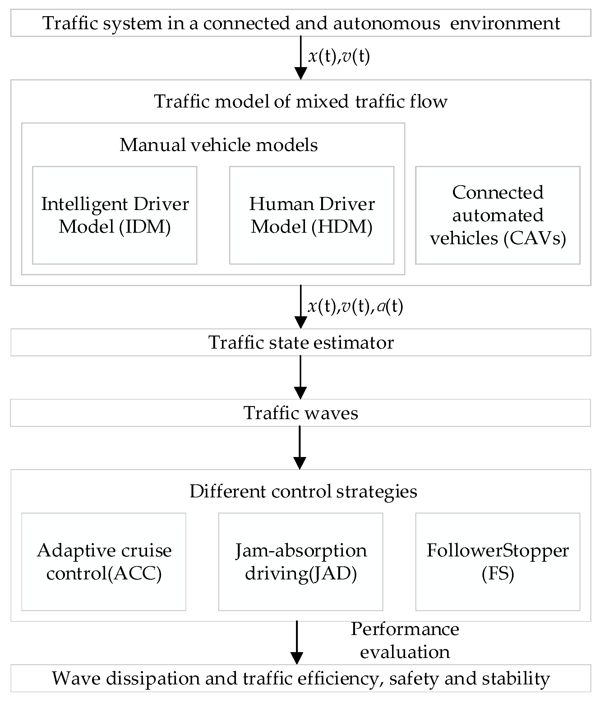
To evaluate the effectiveness of different methods, a simulation framework is established, as shown in Figure 1. We consider microscopic traffic models, which describe the system entities and their interactions in detail, treating each vehicle as a separate agent within a network [31]. A large number of studies have tried to explain the spread of traffic shockwaves using the car-following model. For manual vehicles, IDM and HDM are selected. IDM [32] is a collision-free model that can describe the car-following phenomenon accurately and smooth traffic flow. It allows for the evaluation of different traffic management strategies and their impact on traffic flow. In addition, the HDM is an extension of the IDM that takes into account the impact of human factors, such as reaction time, estimation errors, and temporal anticipation. Most importantly, it provides a more realistic representation of driver behavior than the IDM in certain situations. The HDM model and CAVs model can be found in Appendix A. The different control strategies (the ACC, FS, and JAD strategies can be found in Appendix B) are implemented for each vehicle using MATLAB to allow data transmission within the framework.
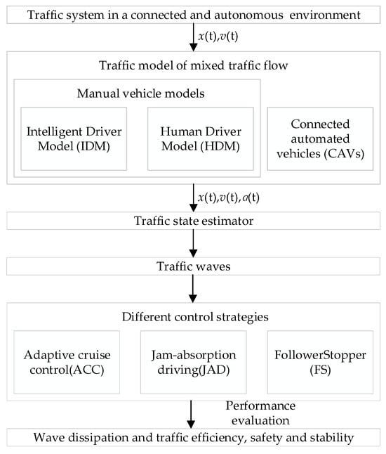
Figure 1.
Overview of the simulation framework.
3. Experimental Set-Up
To evaluate the effectiveness and practicability of these three methods (ACC, FS, and JAD) in mixed traffic, circular and linear roads were chosen. In the experiment, the IDM model and HDM model are employed for manual vehicles, respectively. In the experiment, the parameters of the IDM model and HDM model are set in Table 1 and Table 2. These parameters are used in our experiments and refer to the literature, where they have been taken from [33].

Table 1.
Parameters of the intelligent driver model (IDM).
Table 2.
Parameters of the human driver model (HDM).
To simplify the different control strategies based on different car-following models, they can be written into six modes: ACC-IDM, ACC-HDM, FS-IDM, FS-HDM, JAD-IDM, and JAD-HDM. Taking into account the randomness of the simulation experiments, each scenario of the experiment was run 10 times and the results were averaged. The CAV was designated as the guidance vehicle, and the number and placement of these guidance vehicles were identical for different methods.
3.1. Ring-Road
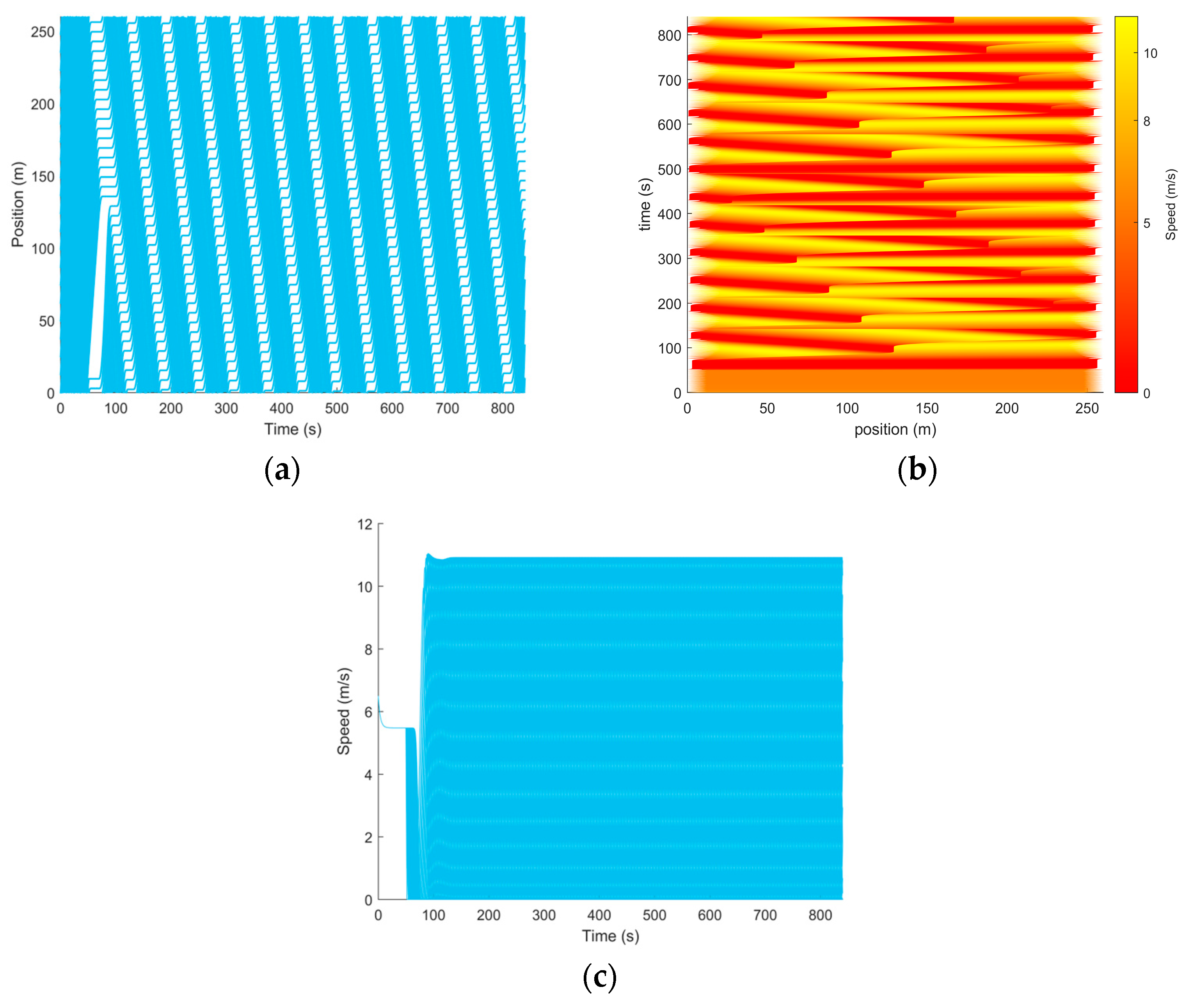
In this experiment, a 260 m single-lane ring road is considered. There are 21 vehicles on the road, including the CAVs. The length of each vehicle is set to an approximate value to facilitate modeling and calculation. And the vehicles are initially evenly spaced within the ring road, as it is depicted in Figure 2. The red and blue vehicles in this figure represent CAVs and manually driven vehicles, respectively. According to the previous literature [34], considering human comfort, the maximum allowable acceleration and deceleration of vehicles are set to 3 m/s2 and −6 m/s2, respectively. The initial velocity of the vehicle was set to 6.5 m/s. All vehicles stopped at 840 s and the simulation time step is 0.01 s. To study the effects of three different methods on traffic performance, a disturbance is introduced into the traffic flow. Specifically, the acceleration of the leading vehicle was set to no more than −3 m/s2 between the 50th and 70th seconds. Hence, the induced perturbation results in a traffic oscillation phenomenon, as shown in Figure 3 and Figure 4. In the experiment, Vehicle 21 was set as the first vehicle. Seven scenarios were set up with different penetration rates of CAVs, as shown in Table 3.
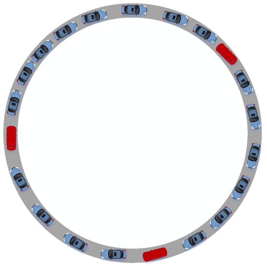
Figure 2.
The schematic diagram of a single-lane ring road: the red and blue vehicles represent CAVs and manually driven vehicles, respectively.
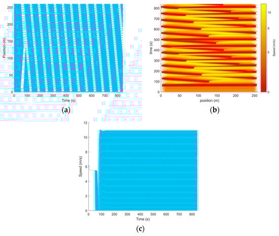
Figure 3.
The diagrams of trajectories based on the IDM model: (a) vehicle trajectories; (b) pseudo-color map of vehicle trajectories; (c) speed trajectories.
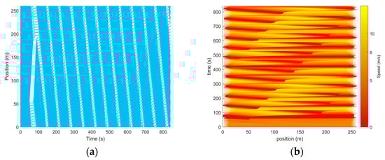

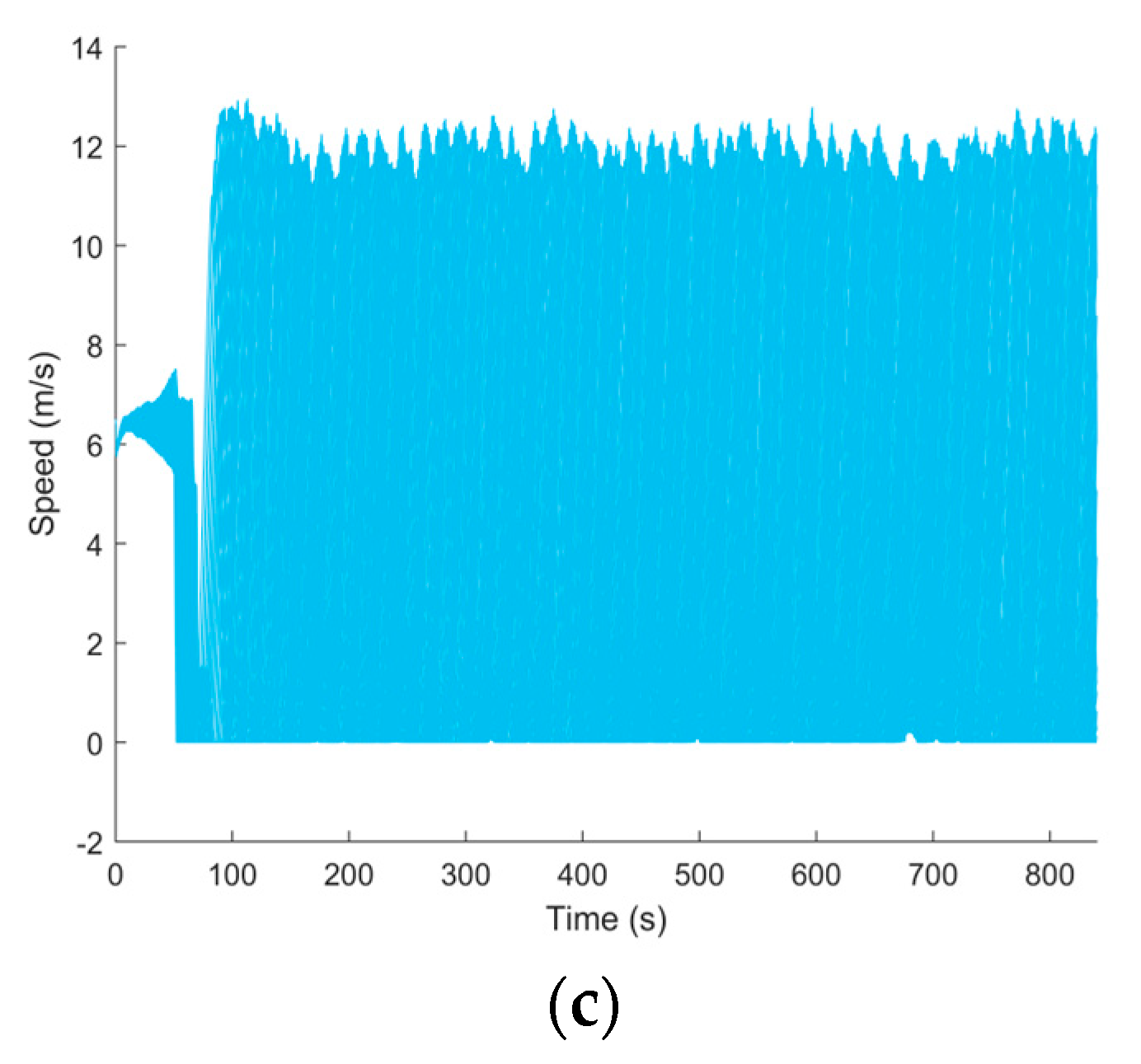
Figure 4.
The diagrams of trajectories based on the HDM model: (a) vehicle trajectories; (b) pseudo-color map of vehicle trajectories; (c) speed trajectories.
Table 3.
Experimental scenario on the ring road.
3.2. Freeway Stretch
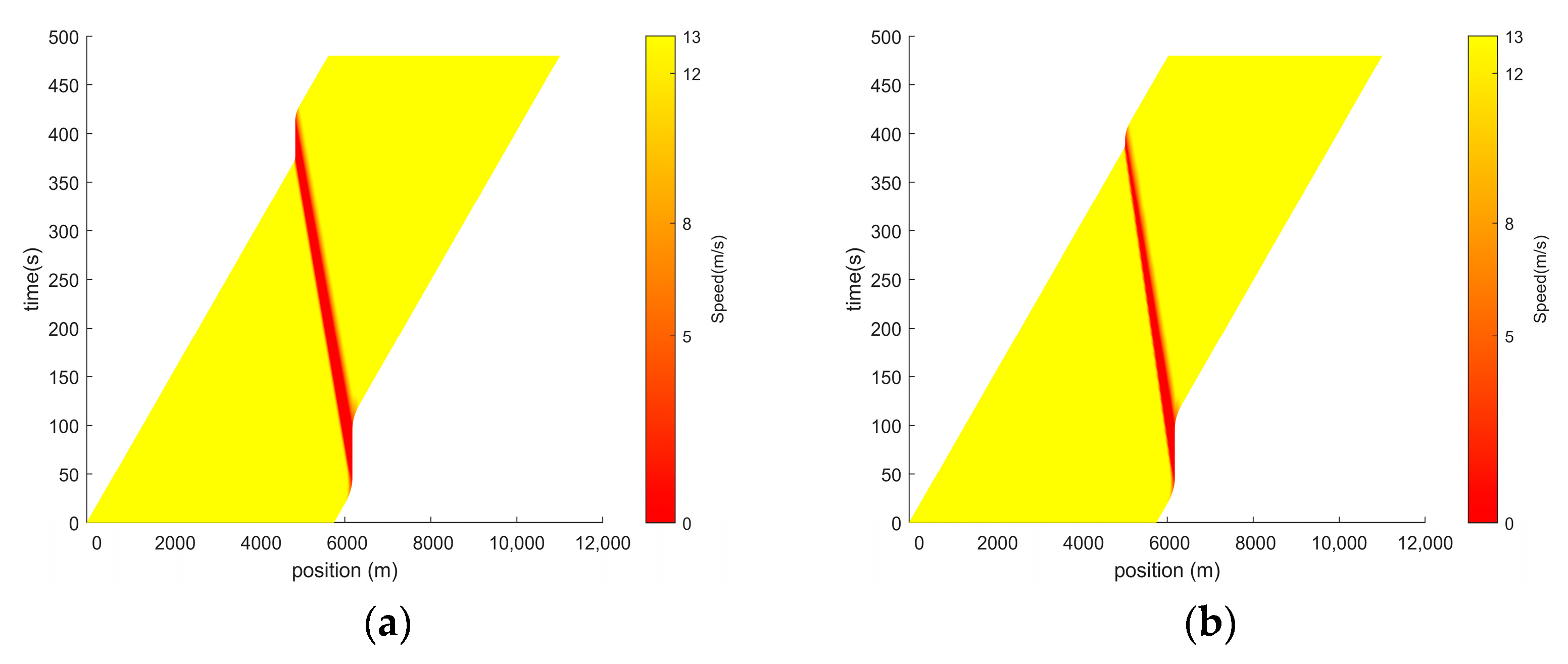
The simulated road is a 7 km one-lane roadway without on-ramps and off-ramps. There are 200 vehicles on the road, including the CAVs. Initially, the distance between vehicles is set to 24 m. The total simulated time is 480 s, and other parameters are the same as those of the ring road. The schematic diagram is shown in Figure 5. The red and blue vehicles are the same as depicted in Figure 2. Accordingly, a speed perturbation is implemented to examine traffic performance in the traffic flow. To be specific, when the traffic is in equilibrium, the leading vehicle slows down for 46 s, and the subsequent vehicle accelerates again. The space–time diagram of speed for the IDM model and HDM model is shown in Figure 6. In the experiment, Vehicle 1 was set as the first vehicle. Different scenarios were established with different penetration rates of CAVs, as indicated in Table 4.

Figure 5.
A schematic diagram of the freeway stretch: the red and blue vehicles represent CAVs and manually driven vehicles, respectively.
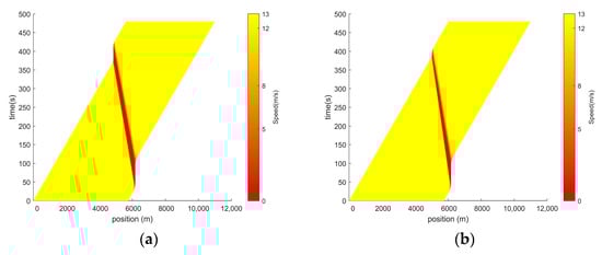
Figure 6.
The space–time diagram of speed without control. (a) IDM model; (b) HDM model.
Table 4.
Experimental scenario on the linear road.
3.3. Definition of Performance Metrics
To evaluate traffic efficiency and stability, statistics on the traffic speed are considered as performance indicators in the traffic flow. At each time instant, the spatial-temporal average instantaneous speed and the speed standard deviation are given as
where is the speed of vehicle n (n = 1, …, N) at a given time indexed by j (j = 1, …,). And is the total simulation time.
The traffic density is computed by the number of all vehicles N divided by the length of the track L as
Accordingly, the traffic throughput is computed as
Similarly, to evaluate the safety performance of the system, two safety evaluation indexes are used: time exposed time-to-collision (TET) and time integrated time-to-collision (TIT). These are based on the time to collision (TTC), which refers to the time required when there is a potential rear-end collision risk between two consecutive vehicles. TTC is a traffic safety indicator used to assess the risk of collisions. Due to its simplicity and reliability, it is widely considered a potential parameter for alert thresholds in collision avoidance systems. Typically, it is employed in driver assistance systems and research on vehicle safety.
where l represents the length of the vehicle and l = 4.9 m. TET stands for the cumulative time during a specified period when potential collisions could occur. It considers the duration of potential collisions, providing a more comprehensive evaluation of traffic safety.
Meanwhile, TIT is a measure that corrects and integrates collision time, taking into consideration variations in vehicle speed and relative distance to more precisely assess the risk of collisions.
According to the previous literature [35], is set to 2 s. TET and TIT are comprehensive indicators of TTC for safety evaluation. Therefore, a lower TET value indicates a safer traffic system, and the lower values of both TET and TIT values indicate a safer traffic system.
4. Results and Discussion
To compare the impact of the different control strategies on traffic waves, the experiment was simulated on a circular road and a linear road.
4.1. A Scenario with a Series of Traffic Oscillations on the Ring Road
4.1.1. The Ring Road with a Single Guidance Vehicle
In the experiment, one single CAV was considered as a guidance vehicle. To assess the traffic efficiency and stability of different modes using IDM and HDM, the average speed, standard deviation of speed, and traffic throughput were calculated, as reported in Table 5 and Table 6, respectively.
Table 5.
The performance metrics of different modes using IDM.
Table 6.
The performance metrics of different modes using HDM.
In Table 5 and Table 6, the uncontrolled scenarios based on the IDM model and HDM model are considered baseline values. It can be observed from Table 5 and Table 6 that the average speed and traffic throughput of different modes were improved to different degrees, while the standard deviation of speed decreased. The numerical results indicated that different modes can reduce traffic waves and improve traffic efficiency and stability when a single CAV is used. Among them, the FS strategy showed the highest increase in average velocity and throughput, as well as the highest reduction in the speed standard deviation. However, the performance improvement of the ACC strategy was minimal. In other words, a CAV equipped with an FS controller provided sufficient dissipation effects and significantly improved the traffic efficiency in this experiment. Compared with the FS controller, the performance improvement became marginal for the ACC and JAD control strategies.
When the manual vehicle is the IDM model, the ACC controller resulted in a 1.10% increase in the average speed, a 0.81% reduction in the speed standard deviation, and a 0.85% rise in the traffic throughput. The average speed was increased by 27.75% and 3.02%, the speed standard deviation was decreased by 58.49% and 9.70%, and the throughput was increased by 27.64% and 4.06% under the FS and JAD methods, respectively. Similarly, it can be seen that the throughput increased by 2.16%, 25.04%, and 5.55%, respectively, for ACC, FS, and JAD when the manual vehicle is the HDM model. The average speed increased by 2.24%, 25.11%, and 5.61% for these three methods, while the speed standard deviation decreased by 2.26%, 57.14%, and 13.16%, respectively. The results indicate that the performance of the strategy is related to the car-following model.
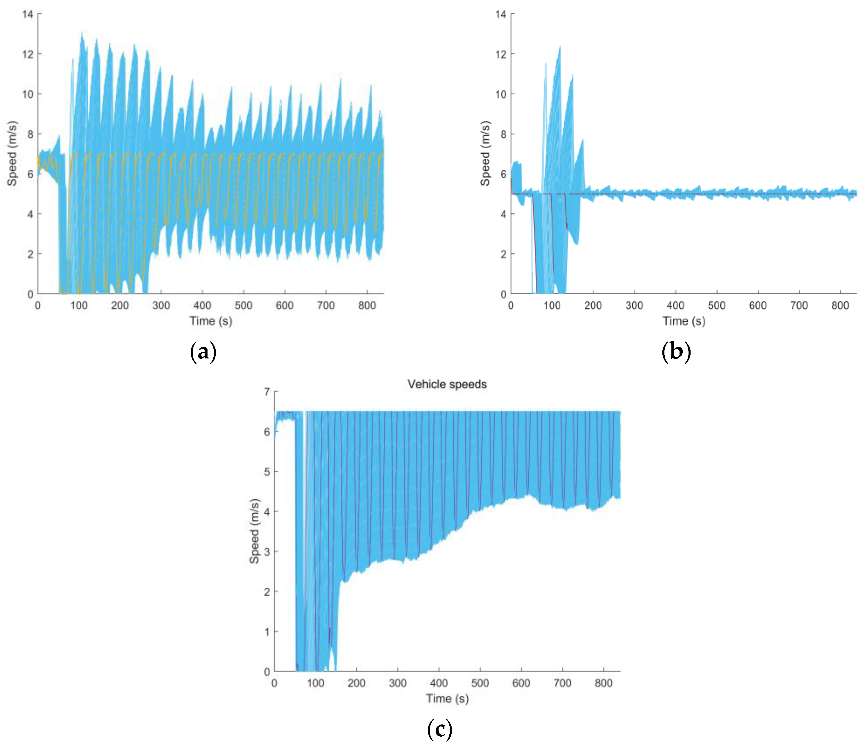
In mixed traffic flow, the speed trajectories for different strategies are plotted according to the experimental parameters. When the manual vehicle is the IDM model and HDM model, the speed trajectories for different control strategies are shown in Figure 7 and Figure 8, respectively. In these figures, the blue line represents manual vehicles and the CAV guidance vehicle is represented in other colors for the different control strategies.
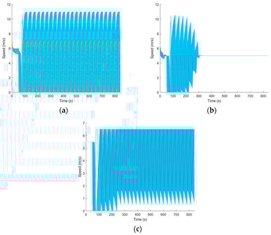
Figure 7.
The speed trajectories based on the IDM model under different control strategies. (a) ACC (The blue line represents manual vehicles, and the CAV guidance vehicle is represented in orange color); (b) FS (The blue line represents manual vehicles, and the CAV guidance vehicle is represented in red color); (c) JAD (The blue line represents manual vehicles, and the CAV guidance vehicles is represented in purple color).

Figure 8.
The speed trajectories based on the HDM model under the different control strategies. (a) ACC (The blue line represents manual vehicles, and the CAV guidance vehicle is represented in orange color); (b) FS (The blue line represents manual vehicles, and the CAV guidance vehicle is represented in red color); (c) JAD (The blue line represents manual vehicles, and the CAV guidance vehicle is represented in purple color).
Figure 7 and Figure 8 depict that it is evident that the speed trajectory of the FS strategy stabilized around a constant value compared with other strategies. This revealed that the stop-and-go waves were effectively suppressed with one CAV under the FS strategy. The percentage change in safety evaluation metrics was quantified in the experiment, as shown in Table 7.
Table 7.
The percentage change in safety evaluation metrics.
It can be seen from Table 7 that the safety indicators of TET and TIT for different modes were reduced, which indicates that their traffic safety performance has been improved. Among them, the FS-IDM mode led to a decrease of 35.36% and 35.91% in TET and TIT, respectively, and it was the most improved among the six modes. This suggests that the FS-IDM mode demonstrates the best traffic safety performance when there is only one CAV guidance vehicle. In addition, for different car-following models, the ACC and JAD strategies based on the HDM model exhibited a superior performance in terms of traffic safety, while the FS strategy based on the IDM model showed a lower rear-end collision risk.
The analysis presented above indicated that when employing a single CAV, the FS controller exhibited the most noticeable enhancement in traffic efficiency, stability, and safety, followed by the JAD strategy, with the ACC approach showing the least substantial performance improvement. Additionally, when employing the same strategy and comparing different car-following models, it is evident that the ACC and JAD strategies based on the HDM model outperformed in traffic performance, while the FS strategy based on the IDM model led to optimal traffic performance. This might be related to the adaptability and advantages of the strategies.
4.1.2. The Ring Road with Multiple Guidance Vehicles
To evaluate the traffic performance of the system based on different car-following models under different control strategies, different scenarios with multiple CAVs were tested. Table 8 shows the improvement rate of traffic throughput. For the ACC system, with the increase in the penetration rates of CAVs, traffic throughput showed an increasing trend. For the JAD strategy, as the percentage of CAVs increased from 4% to 40%, the throughput gradually increased. However, the improvement in throughput for the JAD strategy became marginal when the percentage of CAVs exceeded 40%. For the FS strategy, when the proportion of CAVs increased to 9%, the throughput reached maximum values. However, as the proportion of CAVs exceeded 9%, the throughput started to gradually decrease. This indicated that the introduction of multiple CAVs for the ACC system can improve traffic efficiency and make traffic waves smoother. In addition, the JAD strategy exhibited robustness, and a higher number of CAVs may be advantageous for traffic wave dissipation and improving traffic efficiency. However, as the proportion of CAVs increases, the FS strategy has a negative impact on traffic efficiency. Moreover, in terms of traffic efficiency, the FS strategy demonstrated the maximum improvement at a 9% CAVs ratio, followed by a slightly lower improvement at a 40% CAVs ratio, while ACC with 50% CAVs showed a lower level of enhancement.
Table 8.
The improvement rate of traffic throughput.
At the same time, for different car-following models, the ACC and JAD strategies based on the HDM model exhibited a superior performance in terms of traffic efficiency, while the FS strategy based on the IDM model performed optimally in traffic efficiency.
The reduction in the speed standard deviation for different penetration rates of CAVs under all six modes was reported in Table 9. The improvement trend in traffic throughput for ACC and JAD aligned consistently with the corresponding decreasing trend in the speed standard deviation. In contrast, for the FS strategy, as the CAV proportion increased from 4% to 20%, the speed standard deviation decreased by 65.50%. However, when the CAV proportion exceeded 20%, the reduction in the speed standard deviation diminished to 59.57%.
Table 9.
The reduction in speed standard deviation for different modes.
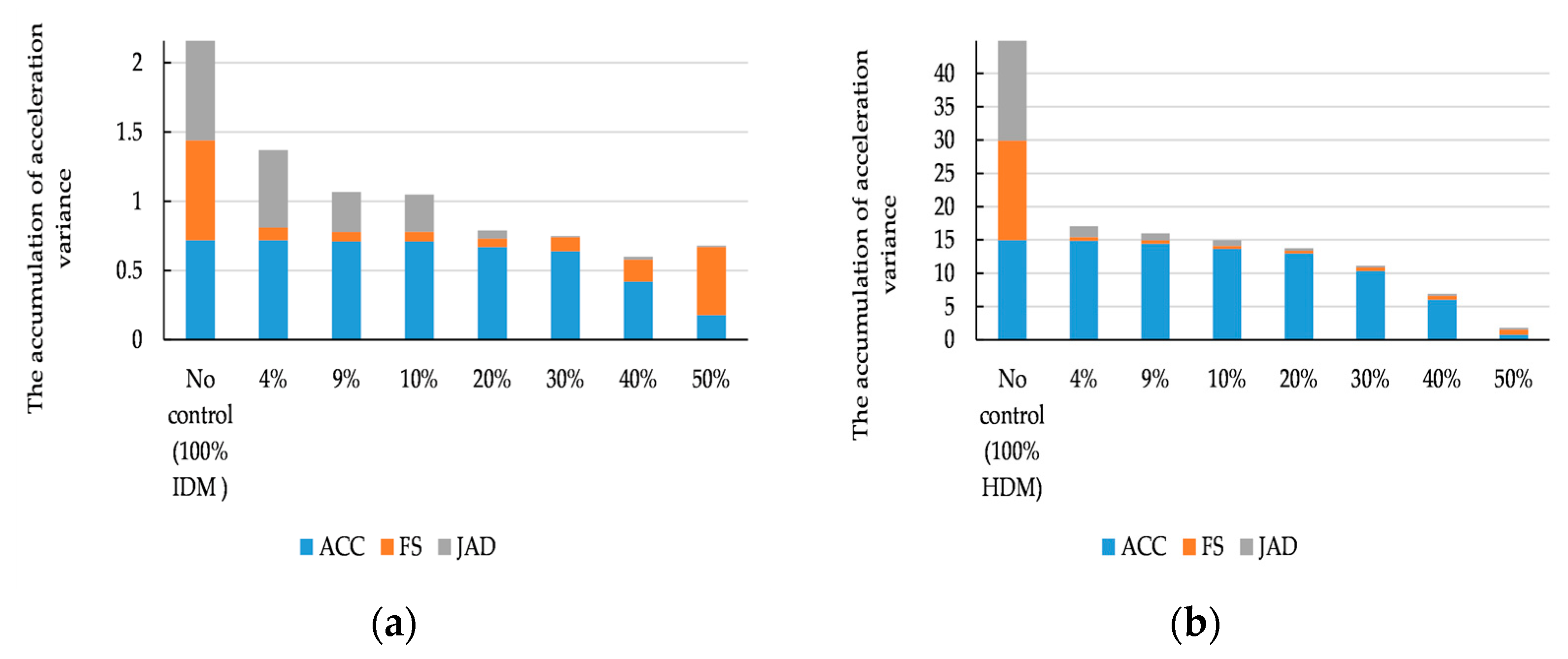
The distribution of acceleration variance is shown in Figure 9. It showed that there was a decrease in the acceleration variance compared to the uncontrolled situation. The trends in acceleration variance corresponding to different following models were similar. Additionally, the distribution of acceleration variance demonstrated that its trend is consistent with the speed standard deviation reduction trend.

Figure 9.
The acceleration variance for different car-following models. (a) IDM model; (b) HDM model.
The changes in TET and TIT of different modes with the penetration rates of CAVs were quantified in Table 10 and Table 11. The numerical findings revealed that there are variations in TET and TIT for different modes when using different car-following models. Specifically, at the lowest proportion of CAVs, the reduction rates of safety indicators (TET and TIT) for various modes were minimal, suggesting that the safety level is relatively lower in the mixed traffic. When the proportion of CAVs reaches 50%, the reduction rates of TET and TIT for the ACC system based on HDM were maximized at 58.72% and 58.81%, respectively. This indicated a higher level of traffic safety for the HDM-based ACC system. With the FS strategy, as the penetration rates of CAVs increased, the reduction rates of TET and TIT rose when the proportion of CAVs was below 20%. However, once the proportion of CAVs surpassed 20%, the traffic safety level declined. When the penetration rate of CAVs was 20%, the safety indicators for the FS strategy based on the IDM model exhibited reduction rates of 71.80% and 71.82%, respectively. For the JAD strategy, as the proportion of CAVs increased, its safety performance improved, but this enhancement was not infinite. Specifically, as the proportion of CAVs increased from 40% to 50%, the improvement in safety performance stabilized at approximately constant values. Hence, for the HDM model, the improvement amounts were around 61.91% and 61.90%. Because the JAD strategy can mitigate secondary waves, and as observed in the table data, the vehicle risk diminished with the growing proportion of CAVs. This suggested that the JAD strategy is robust for various car-following models.
Table 10.
The reduction in TET and TIT for the system using the IDM model.
Table 11.
The reduction in TET and TIT for the system using the HDM model.
From the analysis above, it can be concluded that the introduction of more CAVs may have a positive impact on traffic performance for the ACC strategy. Specifically, when the penetration rate of CAVs reaches 50%, the ACC strategy can significantly reduce traffic waves and improve traffic performance. Similarly, it confirmed that more FS vehicles may suppress traffic waves at the expense of reducing system flow, thereby negating the benefit of wave dissipation. Furthermore, it showed that the introduction of multiple FS vehicles may have a negative impact on traffic performance. This result was in line with the empirical findings of a single-lane ring road with multiple CAVs driven by the FS controller [30]. Furthermore, it confirmed that the JAD is robust for these two car-following models and more CAVs may be beneficial to wave dissipation, traffic efficiency, and traffic safety [22].
Comparing these three methods, when the penetration rates of CAVs were 50% and 40%, respectively, the ACC and JAD strategies demonstrated the most optimal performance improvements. For the FS strategy, the highest level of traffic efficiency was attained at a CAV proportion of 9%, whereas the optimum traffic stability and safety were achieved when the CAV proportion was 20%. This is because the decreased flow with more FS vehicles can be linked to the slower speed recovery exhibited by FS vehicles, and the system may be a threshold to dampen traffic waves. To put it differently, the FS strategy with the lower CAVs can attain optimal traffic performance, followed by the JAD strategy, whereas the ACC strategy requires the most CAVs to achieve optimal traffic performance. In terms of the car-following model, ACC and JAD strategies based on the HDM model exhibited a superior traffic performance, while a system employing the IDM model demonstrated better overall performance indicators for the FS strategy. The reasons behind these results may be attributed to the adaptability and advantages of the HDM and IDM models under different strategies.
4.2. A Scenario with the Traffic Oscillation on the Freeway Stretch
4.2.1. A Guidance Vehicle
To compare the traffic performance of different modes, the numerical experiments were tested on the linear road. The parameters of performance metrics with one guidance vehicle were reported in Table 12. It is clear from Table 12 that the inclusion of a CAV in both the ACC strategy and JAD strategy led to a reduction in speed standard deviation to varying degrees, while also improving average speed and throughput. These results are similar to those of the circular road, with the difference being that the FS strategy had a negative impact on performance metrics Specifically, under the ACC and JAD strategies based on the IDM model, the average speed increased by 0.18%, and 6.32%, the speed standard deviation decreased by a 1.46% and 38.11%, and the throughput increased by 0.24% and 6.3% respectively. Similarly, under the ACC and JAD strategies based on the HDM model, there were respective increases of 0.17% and 3.48% in average speed, while speed standard deviation decreased by 1.11% and 31.48%, and throughput increased by 0.18% and 3.52%.
Table 12.
The parameters of performance metrics with one CAV vehicle.
The safety evaluation indexes for different modes were calculated, as reported in Table 13. The results indicated that when only one CAV served as the guidance vehicle, both the ACC and JAD strategies contributed to a decrease in TET and TIT, while the FS strategy led to an increment in both TET and TIT. In the JAD-IDM mode, there was a 7.49% reduction in TET and a 7.52% reduction in TIT, with the JAD-IDM mode showing the highest reduction in TET and TIT. Hence, a comparison of the ACC, FS, and JAD strategies revealed that the JAD strategy performed the best in terms of traffic safety, followed by ACC, while the FS strategy exhibited the highest rear-end collision risk. Additionally, when using the same strategy, it is evident that rear-end crash risk in the system based on IDM was significantly lower than in the system based on HDM, indicating that the IDM-based system showed a superior level of traffic safety.
Table 13.
The safety evaluation metrics for different modes.
Based on the analysis above, it can be concluded that compared to the HDM-based system, the IDM-based system is likely to improve traffic performance and wave dissipation. In mixed traffic flow, the JAD strategy demonstrated the best traffic performance, followed by ACC, while the FS strategy exhibited a deteriorating traffic performance.
4.2.2. Multiple Guidance Vehicles
When introducing multiple CAVs, experimental simulations were conducted to obtain traffic throughput in mixed traffic using different control strategies based on various car-following models, as depicted in Figure 10. It indicated a substantial increase in throughput for different penetration rates of CAVs under both the ACC and JAD strategies, whereas the FS strategy led to a reduction in throughput. Specifically, the throughput increased with the addition of CAVs for the ACC strategy. When the number of CAVs reached 20%, the throughput was maximized, and further improvements in throughput with an increase in the number of CAVs became marginal. However, the FS strategy led to an increase in traffic throughput. Furthermore, the changes in throughput exhibited a similar pattern for the different car-following models. It is clear that the system using the IDM model resulted in more significant enhancements in throughput compared to the HDM model.
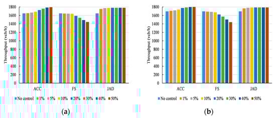
Figure 10.
The traffic throughput for different control strategies. (a) IDM model; (b) HDM model.
The variation in the speed standard deviation for different modes was quantified in Table 14. Based on the data results, it can be observed that the trend in speed standard deviation for different strategies was the opposite to the trend in traffic throughput. When the penetration rate of CAVs reached 20%, the JAD strategy resulted in a significant reduction in the speed standard deviation. Furthermore, with an increase in the penetration rate of CAVs, the improvement in the speed standard deviation under the JAD strategy became negligible. Interestingly, the JAD strategy showed greater improvements in the speed standard deviation compared to the ACC strategy. When the proportion of CAVs reached 50%, the speed standard deviation under the ACC strategy, with IDM and HDM as the manual vehicles, decreased by 36.55% and 27.30%, respectively. Similarly, with the 20% CAVs, the speed standard deviation under the JAD strategy decreased by 54.37% and 48.19% for the IDM model and HDM model, respectively. Furthermore, it can be observed that for different car-following models, the improvement in speed standard deviation was greater in the system using the IDM model compared to those using the HDM model.
Table 14.
The variation in the speed standard deviation with different proportions of CAVs.
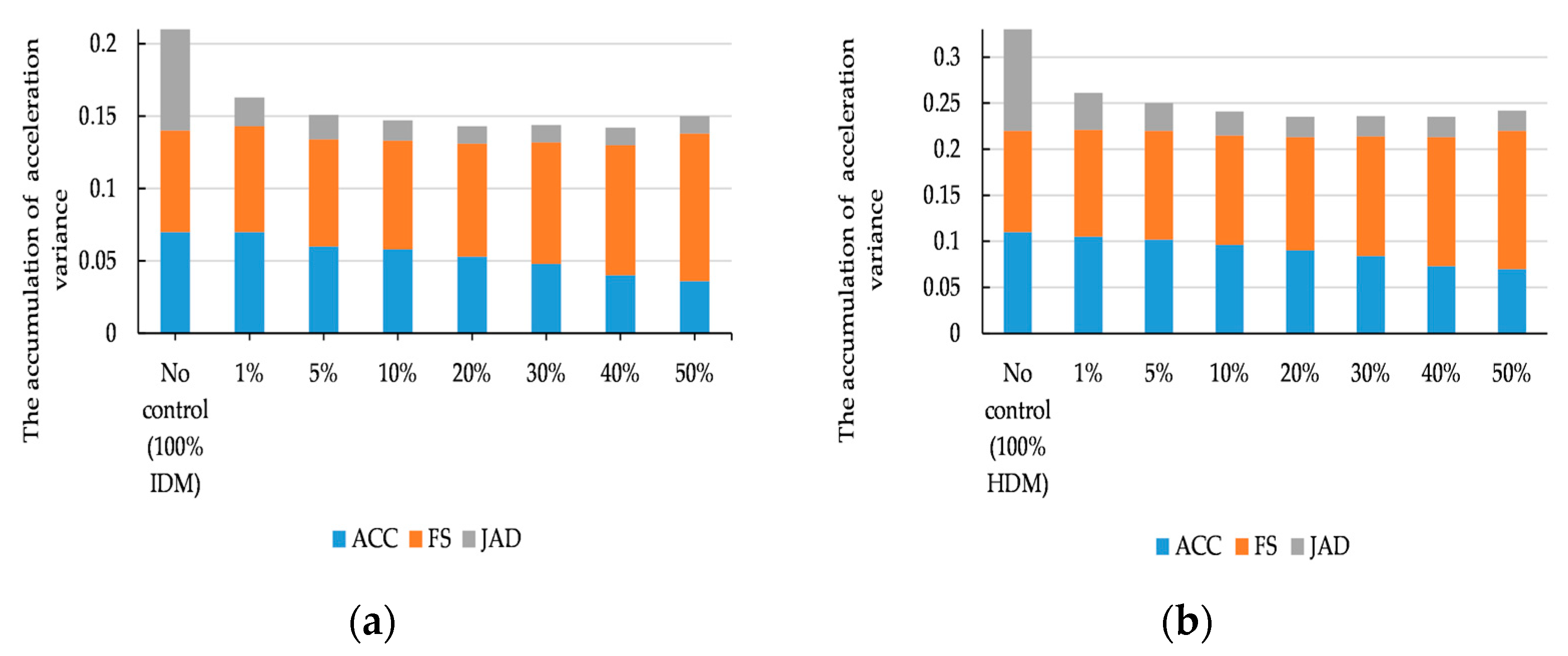
The distribution of acceleration variance is shown in Figure 11. Due to the similarity between the trend of the speed standard deviation and the trend of acceleration variance, it further confirmed that the ACC and JAD strategies are effective in reducing traffic waves and stabilizing traffic flow.
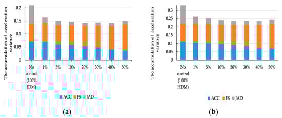
Figure 11.
The distribution of acceleration variance. (a) IDM model; (b) HDM model.
Based on the simulation results, traffic safety indicators were calculated for different modes, as shown in Table 15 and Table 16. Table 15 revealed a gradual increase in TET and TIT with increasing penetration rates of CAVs for the ACC and JAD strategies. This implied that, in mixed traffic flow with the application of ACC and JAD strategies, traffic safety gradually improved as the penetration of CAVs increased. Furthermore, at 50% CAVs, the JAD-IDM mode demonstrated reductions of 69.43% and 69.40% in the TET and TIT safety indicators, respectively. Notably, the JAD-IDM mode exhibits the highest percentage reduction, suggesting that the JAD strategy minimized the risk of rear-end collisions, thereby improving the traffic safety performance. For the FS strategy, the changes in TET and TIT increased with the rising penetration rates of CAVs and exhibited some fluctuations. The fluctuations may be attributed to the introduction of CAVs for the FS strategy, causing additional disturbances that led to small perturbations between vehicles propagating upstream, which failed to eliminate traffic waves and may induce traffic safety issues. The changing trends of TET and TIT for different modes in Table 16 exhibit similarities with the trends of safety indicators in Table 15.
Table 15.
The reduction in traffic safety indicators for the IDM model system.
Table 16.
The reduction in traffic safety indicators for the HDM model system.
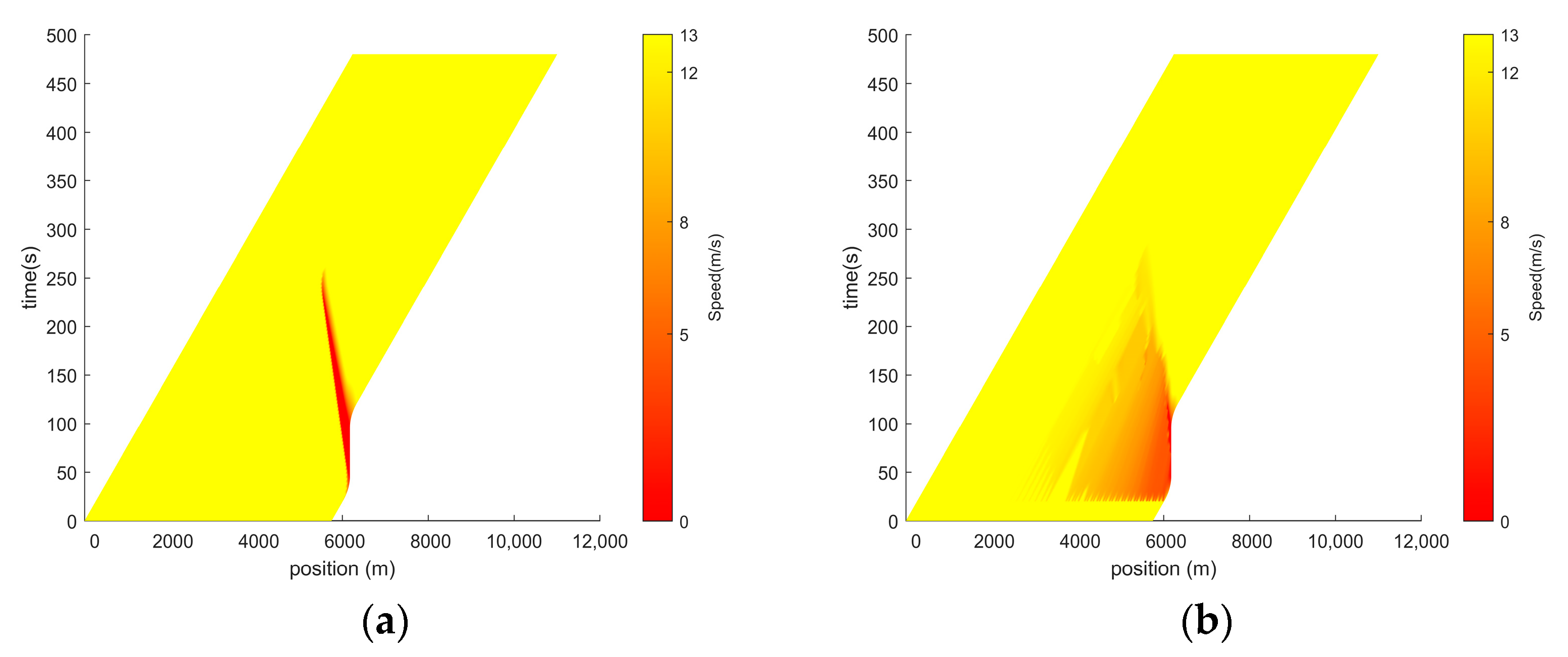
Based on the numerical analysis above, it can be concluded that the JAD strategy with 20% CAVs had the best traffic performance compared to the ACC strategy, as shown in Figure 12. In other words, the JAD strategy can remarkably reduce traffic waves and improve traffic efficiency, stability, and safety. The reason is that the JAD strategy is robust and avoids the generation of secondary waves. Multiple FS vehicles cannot efficiently dissipate traffic waves due to the absence of a large gap as a buffer. This is due to the fact that the mechanism of the FS strategy involves successive passes of the same wave until it dissipates. Conversely, on a linear road, each of the multiple FS vehicles will encounter the same wave once, resulting in just a single pass. In terms of the car-following model, the IDM model exhibited a better traffic performance compared to the HDM model, which was attributed to the dynamic characteristics of the IDM model.
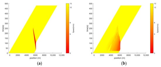
Figure 12.
The space diagram of speed based on the IDM model for different strategies. (a) 50% CAVs under the ACC; (b) 20% CAVs under the JAD.
5. Conclusions and Further Research
This paper compared the effectiveness of the ACC, FS, and JAD control strategies for different car-following models in mixed traffic. By comparing and analyzing numerical results, different control strategies have different effects on traffic performance on the ring and linear road.
The results suggested that on the ring road, the ACC and JAD strategies with multiple CAVs (guidance vehicles) can effectively reduce traffic waves and improve traffic efficiency, stability, and safety. Among these, as the number of CAVs increased, the traffic performance of the ACC strategy gradually improved. Moreover, an increased number of CAVs may potentially improve traffic performance, yet this enhancement was not limitless. In this experiment, the optimal performance for the JAD strategy was achieved with approximately 40% CAVs (guidance vehicles). In contrast, the results indicated that multiple FS vehicles can suppress traffic oscillations, but at the cost of reducing system flow. Interestingly, a lower number of guidance vehicles in the FS strategy can achieve an optimal traffic performance, followed by the JAD strategy, whereas the ACC strategy requires the most guidance vehicles to achieve optimal traffic performance. Furthermore, when manual vehicles are represented by HDM, both ACC and JAD strategies prove more effective in suppressing traffic waves and enhancing traffic performance. Conversely, with manual vehicles modeled by IDM, the FS strategy exhibits relative superiority in stabilizing traffic flow and improving traffic waves compared to other strategies. This could be attributed to the adaptability and strengths of the models.
For the freeway stretch, the experimental results demonstrated that compared to the ACC, having fewer CAVs enables the JAD strategy to effectively reduce traffic waves and enhance traffic efficiency and safety, thereby stabilizing traffic flow. This is mainly because the JAD strategy exhibited robustness and effectively avoided the secondary waves, resulting in substantial improvements in traffic safety. In this experiment, the optimal performance for the JAD strategy was achieved with approximately 20% CAVs (guidance vehicles). Conversely, the FS strategy cannot dissipate traffic waves due to an insufficient buffer gap. Additionally, when manual vehicles are modeled using IDM, both ACC and JAD strategies demonstrated a better suppression of traffic waves and an improvement in traffic performance. This could be attributed to the dynamic characteristics of the IDM model.
This experiment assessed the impact of different control strategies on mixed traffic flow on a single-lane circular road and freeway. In mixed traffic, CAVs utilize onboard sensors to capture the real-time position and speed information of the vehicle, subsequently transmitting these data to the traffic management center through the roadside communication system. The processing system evaluates the traffic information to ascertain whether traffic waves are occurring on the road. Once the phenomenon is detected, the control strategy is triggered. According to the level of road congestion and the number of CAVs, an appropriate control strategy is selected to alleviate traffic waves. This holds theoretical significance for the selection and decision of the control strategy equipped with CAVs on the ring road and freeway to reduce traffic congestion.
In the future, it will be imperative to implement and test different control strategies in multi-lane or more complex situations to approximate more realistic traffic. Simultaneously, taking into account factors like traffic efficiency, traffic safety, and pollution emissions is crucial for achieving optimal control. This holds significant importance in reducing traffic congestion and improving control efficiency.
Author Contributions
Conceptualization, C.R. and W.Z.; methodology, H.L.; software, H.L.; validation, H.L., C.R. and Y.J. All authors have read and agreed to the published version of the manuscript.
Funding
This research received no external funding.
Institutional Review Board Statement
Not applicable.
Informed Consent Statement
Not applicable.
Data Availability Statement
Data is contained within the article.
Conflicts of Interest
The authors declare no conflicts of interest.
Appendix A
Appendix A.1. Human Driver Model (HDM)
Based on IDM, the model introduces a series of factors such as the driver’s reaction time, estimation errors, and temporal anticipation to better simulate human driving behavior. The vehicle acceleration of the HDM can be calculated as
where and are the free-flow and interaction accelerations, respectively. Their definitions are described in the following equations:
where is a linear forward projection of the gap in temporal anticipation, and is a linear forward projection of the speed during the reaction time in temporal anticipation. And . Specifically, and are given by
where and are the estimation error of the gap and the speed of the leading vehicle, is the reaction time, and . and can be written as follows:
where is the relative standard deviation of from the true value s, also known as the statistical variation coefficient of the gap is the temporal evolution of the error, (0,1)-normally distributed stochastic variable, represents the distribution of the error and its change in time, denotes estimation error for the inverse time-to-collision (TTC). The parameter is the hypothetic time interval to a collision if neither vehicle accelerates or brakes and can be expressed as follows:
In addition, the Wiener process is used for the time dependence of the estimation errors, and the update rule is given by
where is the persistence time of the estimation errors, are instances of computer-generated pseudo-random numbers with an expectation of zero and unit variance. In other words, it means and , respectively. denotes the independent Wiener processes and for each driver which are initialized using the pseudo-random number generator. Specifically, it can be expressed as follows:
Appendix A.2. CAV Model
Thanks to V2V communication technology, CACC-equipped vehicles can access operational data between vehicles, automatically adjusting the spacing between vehicles based on the position and speed of the leading vehicle. Consequently, it is employed to represent the characteristics of CAVs. The model is described as
where is the speed of the vehicle at time , and are control gains, denotes the error term between the actual spacing and the desired spacing of the preceding and following vehicles. is the headway between vehicles, and is the desired time headway. The first-order Taylor expansion of Equations (A14) and (A15) yields the following acceleration equation:
According to the literature [36], these parameters are assigned the following values: = 0.45 s−1, = 0.25 s−1, = 0.6 s, and = 0.01 s.
Appendix B
Appendix B.1. Adaptive Cruise Control (ACC)
An ACC controller can measure the actual distance and speed difference for a preceding vehicle. These input data and the vehicle’s own speed enable the system to calculate the required acceleration or deceleration to maintain a specific time gap, achieve the desired speed, or prevent traffic collision. Specifically, the typical ACC control algorithm is described as follows:
where s is the vehicle spacing, and are the control gain, and are the desired time-headway and desired speed. and are the accelerations of gap mode and cruise mode under ACC control, respectively. The acceleration satisfies . In the experiment, the desired time headway and the control gain and were set to 0.8 s, 5, and 0.4, respectively, as suggested by the previous study [37].
Appendix B.2. FollowerStopper (FS) Strategy
It is the AVs equipped with the FS controller that produce an appropriate gap to dissipate traffic waves. In the FS strategy, CAVs degenerate into AVs to simulate experiments [38]. CAVs can employ sensors for detecting the distance to the preceding vehicles, enabling the measurement of the speed difference between them. According to the principle of FS, the – phase space diagram can be divided into four regions. Hence, and can be described as follows:
The core of the control strategy is to determine the command speed of CAVs. According to the basic relationship of the region boundaries, the command speed can be given by
where is the desired velocity, (where = 1, 2, 3) is the boundary between the four regions. is the leading vehicle velocity or the desired velocity, whichever is lower. and can be expressed as follows:
where is the intercept of parabolic boundaries between regions, and is vehicle deceleration rate. is the negative arm of the velocity difference and is defined as follows:
To smooth the acceleration profile of CAVs and approach the real environment, the dynamic acceleration update rules in the FS control strategy are as follows:
And acceleration satisfies the following condition:
In addition, when the updated command speed of CAVs is less than the previous command speed of CAVs, the acceleration update rule is given by
where , , , and represent the upper and lower bounds of and , respectively. If the acceleration is not satisfied in Formula (A28), the acceleration update rule is as follows:
To determine the command speed, these parameters are set as shown in Table A1 [39]. Among them, the desired speed U is set to 5 m/s.
Table A1.
The parameters of the FollowerStopper strategy.
Table A1.
The parameters of the FollowerStopper strategy.
| Parameters | Value |
|---|---|
| 4.5 m | |
| 5.25 m | |
| 6.0 m | |
| 1.5 m/s2 | |
| 1.0 m/s2 | |
| 0.5 m/s2 | |
| U | 5 m/s |
Appendix B.3. Jam-Absorption Driving (JAD)
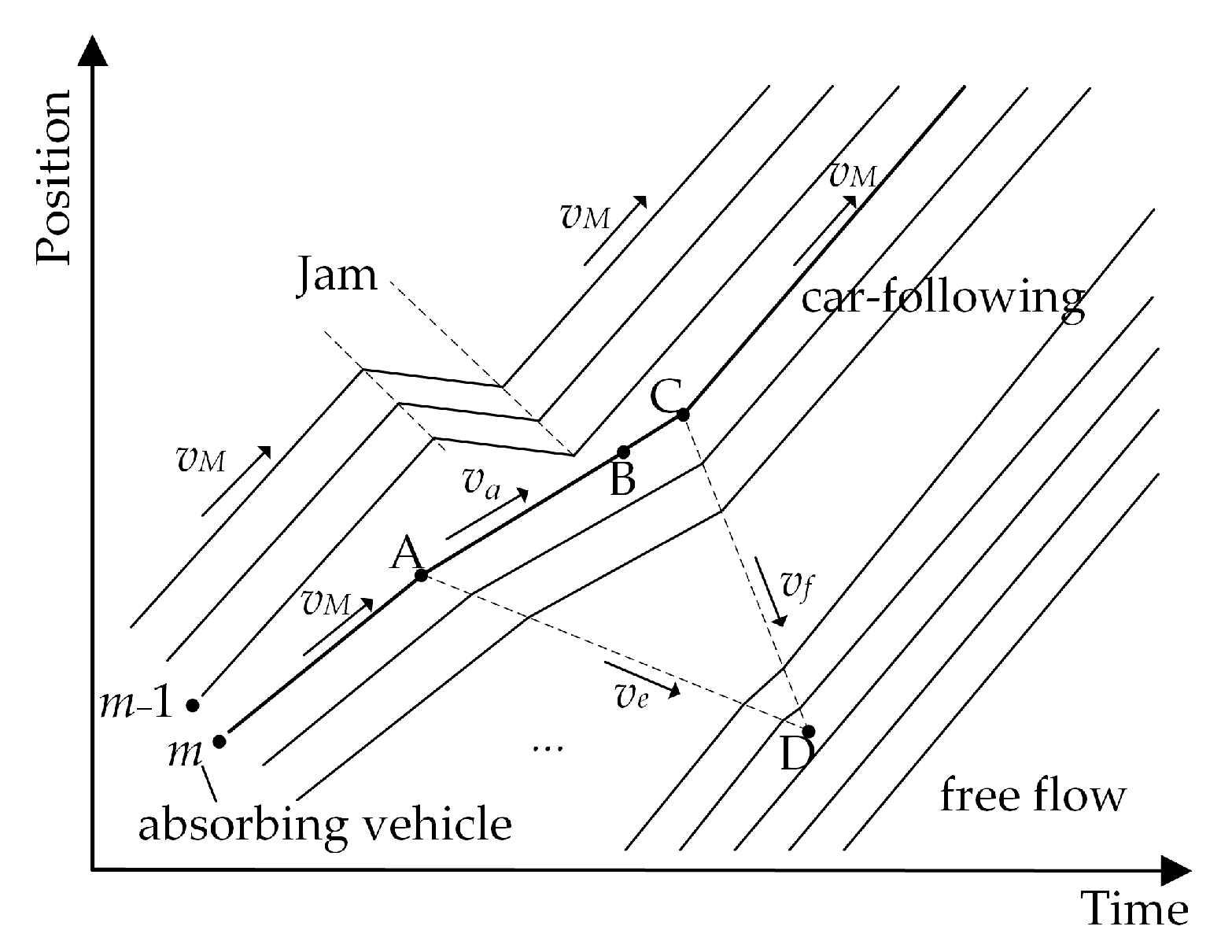
Jam absorption driving is a technique used in vehicle automation and autonomous driving to mitigate the effects of traffic congestion [40]. The key idea of the method is to eliminate traffic jams by dynamically changing the headway of a single vehicle. The schematic diagram is shown in Figure A1.
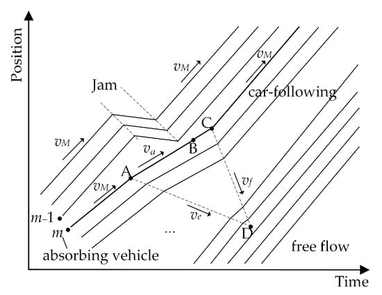
Figure A1.
The schematic diagram of the jam-absorption driving (JAD) strategy.
Figure A1.
The schematic diagram of the jam-absorption driving (JAD) strategy.
References
- Almatar, K.M. Traffic congestion patterns in the urban road network: (Dammam metropolitan area). Ain Shams Eng. J. 2023, 14, 101886. [Google Scholar] [CrossRef]
- Li, X.; Cui, J.; An, S.; Parsafard, M. Stop-and-go traffic analysis: Theoretical properties, environmental impacts and oscillation mitigation. Transp. Res. Part B Methodol. 2014, 70, 319–339. [Google Scholar] [CrossRef]
- Zheng, S.T.; Jiang, R.; Tian, J.; Li, X.; Jia, B.; Gao, Z.; Yu, S. A comparison study on the growth pattern of traffic oscillations in car-following experiments. Transp. B Transp. Dyn. 2023, 11, 706–724. [Google Scholar] [CrossRef]
- Ahn, S.; Laval, J.; Cassidy, M.J. Effects of merging and diverging on freeway traffic oscillations: Theory and observation. Transp. Res. Rec. 2010, 2188, 1–8. [Google Scholar] [CrossRef]
- Chen, D.; Ahn, S. Capacity-drop at extended bottlenecks: Merge, diverge, and weave. Transp. Res. Part B Methodol. 2018, 108, 1–20. [Google Scholar] [CrossRef]
- Li, T.; Ngoduy, D.; Zhao, X. Hopf bifurcation analysis of mixed traffic and its implications for connected and autonomous vehicles. IEEE Trans. Intell. Transp. Syst. 2023, 24, 6542–6557. [Google Scholar] [CrossRef]
- Li, X.; Peng, F.; Ouyang, Y. Measurement and estimation of traffic oscillation properties. Transp. Res. Part B Methodol. 2010, 44, 1–14. [Google Scholar] [CrossRef]
- Chen, D.; Laval, J.A.; Ahn, S.; Zheng, Z. Microscopic traffic hysteresis in traffic oscillations: A behavioral perspective. Transp. Res. Part B Methodol. 2012, 46, 1440–1453. [Google Scholar] [CrossRef]
- Han, Y.; Hegyi, A.; Yuan, Y.; Hoogendoorn, S.; Papageorgiou, M.; Roncoli, C. Resolving freeway jam waves by discrete first-order model-based predictive control of variable speed limits. Transp. Res. Part C Emerg. Technol. 2017, 77, 405–420. [Google Scholar] [CrossRef]
- Müller, E.R.; Carlson, R.C.; Kraus, W.; Papageorgiou, M. Microsimulation analysis of practical aspects of traffic control with variable speed limits. IEEE Trans. Intell. Transp. Syst. 2015, 16, 512–523. [Google Scholar] [CrossRef]
- Li, S.; Cao, D. Variable speed limit strategies’ analysis with cell transmission model on freeway. Mod. Phys. Lett. B 2017, 31, 1750219. [Google Scholar] [CrossRef]
- Grumert, E.; Ma, X.; Tapani, A. Analysis of a cooperative variable speed limit system using microscopic traffic simulation. Transp. Res. Part C Emerg. Technol. 2015, 52, 173–186. [Google Scholar] [CrossRef]
- van de Weg, G.S.; Hegyi, A.; Hoogendoorn, S.P.; De Schutter, B. Efficient freeway MPC by parameterization of ALINEA and a speed-limited area. IEEE Trans. Intell. Transp. Syst. 2018, 20, 16–29. [Google Scholar] [CrossRef]
- Hegyi, A.; Hoogendoorn, S.P. Dynamic speed limit control to resolve shock waves on freeways-Field test results of the SPECIALIST algorithm. In Proceedings of the 13th International IEEE Conference on Intelligent Transportation Systems, Funchal, Portugal, 19–22 September 2010; pp. 519–524. [Google Scholar] [CrossRef]
- Papamichail, I.; Bekiaris-Liberis, N.; Delis, A.I.; Manolis, D.; Mountakis, K.S.; Nikolos, I.K.; Roncoli, C.; Papageorgiou, M. Motorway traffic flow modelling, estimation and control with vehicle automation and communication systems. Annu. Rev. Control 2019, 48, 325–346. [Google Scholar] [CrossRef]
- Roncoli, C.; Papageorgiou, M.; Papamichail, I. Traffic flow optimisation in presence of vehicle automation and communication systems-part II: Optimal control for multi-lane motorways. Transp. Res. Part C Emerg. Technol. 2015, 57, 260–275. [Google Scholar] [CrossRef]
- Roncoli, C.; Papageorgiou, M.; Papamichail, I. Traffic flow optimisation in presence of vehicle automation and communication systems-part I: A first-order multi-lane model for motorway traffic. Transp. Res. Part C Emerg. Technol. 2015, 57, 241–259. [Google Scholar] [CrossRef]
- Perraki, G.; Roncoli, C.; Papamichail, I.; Papageorgiou, M. Evaluation of a model predictive control framework for motorway traffic involving conventional and automated vehicles. Transp. Res. Part C Emerg. Technol. 2018, 92, 456–471. [Google Scholar] [CrossRef]
- Li, Y.; Li, Z.; Wang, H.; Wang, W.; Xing, L. Evaluating the safety impact of adaptive cruise control in traffic oscillations on freeways. Accid. Anal. Prev. 2017, 104, 137–145. [Google Scholar] [CrossRef]
- Li, Y.; Wang, H.; Wang, W.; Xing, L.; Liu, S.; Wei, X. Evaluation of the impacts of cooperative adaptive cruise control on reducing rear-end collision risks on freeways. Accid. Anal. Prev. 2017, 98, 87–95. [Google Scholar] [CrossRef]
- Nishi, R.; Tomoeda, A.; Shimura, K.; Nishinari, K. Theory of jam-absorption driving. Transp. Res. Part B Methodol. 2013, 50, 116–129. [Google Scholar] [CrossRef]
- Taniguchi, Y.; Nishi, R.; Ezaki, T.; Nishinari, K. Jam-absorption driving with a car-following model. Phys. A Stat. Mech. Its Appl. 2015, 433, 304–315. [Google Scholar] [CrossRef]
- He, Z.; Zheng, L.; Song, L.; Zhu, N. A jam-absorption driving strategy for mitigating traffic oscillations. IEEE Trans. Intell. Transp. Syst. 2016, 18, 802–813. [Google Scholar] [CrossRef]
- Tian, J.; Zhu, C.; Chen, D.; Jiang, R.; Wang, G.; Gao, Z. Car following behavioral stochasticity analysis and modeling: Perspective from wave travel time. Transp. Res. Part B Methodol. 2021, 143, 160–176. [Google Scholar] [CrossRef]
- Zheng, Y.; Zhang, G.; Li, Y.; Li, Z. Optimal jam-absorption driving strategy for mitigating rear-end collision risks with oscillations on freeway straight segments. Accid. Anal. Prev. 2020, 135, 105367. [Google Scholar] [CrossRef]
- Nishi, R. Theoretical conditions for restricting secondary jams in jam-absorption driving scenarios. Phys. A Stat. Mech. Its Appl. 2020, 542, 123393. [Google Scholar] [CrossRef]
- Stern, R.E.; Cui, S.; Delle Monache, M.L.; Bhadani, R.; Bunting, M.; Churchill, M.; Hamilton, N.; Pohlmann, H.; Wu, F.; Piccoli, B.; et al. Dissipation of stop-and-go waves via control of autonomous vehicles: Field experiments. Transp. Res. Part C Emerg. Technol. 2018, 89, 205–221. [Google Scholar] [CrossRef]
- Zheng, F.; Lu, L.; Li, R.; Liu, X.; Tang, Y. Traffic oscillation using stochastic lagrangian dynamics: Simulation and mitigation via control of autonomous vehicles. Transp. Res. Rec. 2019, 2673, 1–11. [Google Scholar] [CrossRef]
- Nateeboon, T.; Tawabutr, H.; Termsaithong, T.; Hirunsirisawat, E. Ability to damp traffic wave when controlling every car on the road by FollowerStopper controller. In Proceedings of the Journal of Physics: Conference Series, Siam Physics Congress 2018 (SPC2018), Pitsanulok, Thailand, 21–23 May 2018. [Google Scholar] [CrossRef]
- Cummins, L.; Sun, Y.; Reynolds, M. Simulating the effectiveness of wave dissipation by FollowerStopper autonomous vehicles. Transp. Res. Part C Emerg. Technol. 2021, 123, 102954. [Google Scholar] [CrossRef]
- Nygren, J.; Boij, S.; Rumpler, R.; O’Reilly, C.J. Vehicle-specific noise exposure cost: Noise impact allocation methodology for microscopic traffic simulations. Transp. Res. Part D Transp. Environ. 2023, 118, 103712. [Google Scholar] [CrossRef]
- Treiber, M.; Hennecke, A.; Helbing, D. Congested traffic states in empirical observations and microscopic simulations. Phys. Rev. E 2000, 62, 1805. [Google Scholar] [CrossRef] [PubMed]
- Treiber, M.; Kesting, A. Traffic Flow Dynamics: Data, Models and Simulation, 2013th ed.; Springer: Berlin/Heidelberg, Germany, 2013; pp. 1–505. [Google Scholar] [CrossRef]
- Dias, J.E.A.; Pereira, G.A.S.; Palhares, R.M. Longitudinal model identification and velocity control of an autonomous car. IEEE Trans. Intell. Transp. Syst. 2014, 16, 776–786. [Google Scholar] [CrossRef]
- Das, S.; Maurya, A.K. Defining time-to-collision thresholds by the type of lead vehicle in non-lane-based traffic environments. IEEE Trans. Intell. Transp. Syst. 2020, 21, 4972–4982. [Google Scholar] [CrossRef]
- Milanés, V.; Shladover, S.E. Modeling cooperative and autonomous adaptive cruise control dynamic responses using experimental data. Transp. Res. Part C Emerg. Technol. 2014, 48, 285–300. [Google Scholar] [CrossRef]
- Bekiaris-Liberis, N.; Roncoli, C.; Papageorgiou, M. Predictor-based adaptive cruise control design. IEEE Trans. Intell. Transp. Syst. 2017, 19, 3181–3195. [Google Scholar] [CrossRef]
- Bhadani, R.K.; Piccoli, B.; Seibold, B.; Sprinkle, J.; Work, D. Dissipation of emergent traffic waves in stop-and-go traffic using a supervisory controller. In Proceedings of the 2018 IEEE Conference on Decision and Control (CDC), Miami Beach, FL, USA, 17–19 December 2018; pp. 3628–3633. [Google Scholar] [CrossRef]
- Bhadani, R.; Bunting, M.; Seibold, B.; Stern, R.; Cui, S.; Sprinkle, J.; Work, D.B. Real-time distance estimation and filtering of vehicle headways for smoothing of traffic waves. In Proceedings of the 10th ACM/IEEE International Conference on Cyber-Physical Systems, Montreal, QC, Canada, 16–18 April 2019; pp. 280–290. [Google Scholar] [CrossRef]
- Wang, S.; Li, Z.; Cao, Z.; Jolfaei, A.; Cao, Q. Jam-absorption driving strategy for improving safety near oscillations in a connected vehicle environment considering consequential jams. IEEE Intell. Transp. Syst. Mag. 2021, 14, 41–52. [Google Scholar] [CrossRef]


Disclaimer/Publisher’s Note: The statements, opinions and data contained in all publications are solely those of the individual author(s) and contributor(s) and not of MDPI and/or the editor(s). MDPI and/or the editor(s) disclaim responsibility for any injury to people or property resulting from any ideas, methods, instructions or products referred to in the content. |
© 2024 by the authors. Licensee MDPI, Basel, Switzerland. This article is an open access article distributed under the terms and conditions of the Creative Commons Attribution (CC BY) license (https://creativecommons.org/licenses/by/4.0/).