Using Ensemble Learning for Remote Sensing Inversion of Water Quality Parameters in Poyang Lake

Abstract

Inland bodies of water, such as lakes, play a crucial role in sustaining life and supporting ecosystems. However, with the rapid development of socio-economics, water resources are facing serious pollution problems, such as the eutrophication of water bodies and degradation of wetlands. Therefore, the monitoring, management, and protection of inland water resources are particularly important. In past research, empirical models and machine learning models have been widely used for the water quality assessment of inland lakes. Due to the complexity of the optical properties of inland lake water bodies, the performance of these models is often limited. To overcome the limitations of these models, this study uses in situ water quality data from 2017 to 2018 and multispectral (MS) remote sensing data from Sentinel-2 to construct experimental samples of Poyang Lake. Based on these experimental samples, we constructed a spatio-temporal ensemble model (STE) to evaluate four common water quality parameters: chlorophyll-a (Chl-a), total phosphorus (TP), total nitrogen (TN), and chemical oxygen demand (COD). The model adopts an ensemble learning strategy, improving the model’s performance by merging multiple advanced machine learning algorithms. We introduced several indices related to water quality parameters as auxiliary variables, such as NDCI and Enhanced Three, and used band data and these auxiliary variables as predictive variables, thereby greatly enhancing the predictive potential of the model.The results show that the inversion accuracy of these four inversion models is high ($R^2$ of 0.94, 0.88, 0.92, and 0.93; RMSE of 1.15, 0.01, 0.02, and 0.02; MAE of 0.81, 0.01, 0.09, and 0.10), indicating that the STE model has good evaluation accuracy. Meanwhile, we used the STE model to reveal the spatio-temporal distribution of Chl-a, TP, TN, and COD from 2017 to 2018, and analyzed their seasonal and spatial variation rules. The results of this study not only provide an effective and practical method for monitoring and managing water quality parameters in inland lakes, but also provide water security for socio-economic and ecological environmental safety.

1. Introduction

Lakes, surrounded by land, are surface water bodies typically replenished by rivers, glaciers, precipitation, or groundwater. Although lakes only account for 3.7% of the Earth’s land, they are a crucial component of ecosystems, providing unique living conditions and food chains for many flora and fauna. Simultaneously, lakes play a significant role in hydrological cycles and regional climate regulation [1,2,3,4]. Furthermore, inland water bodies are an essential part of the carbon cycle, contributing to global greenhouse gas emissions [5]. Over the past few decades, due to global warming and human activities, there have been significant changes in the quantity, storage, water surface, and area of inland water resources. An increasing number of lakes are exhibiting environmental problems such as deteriorating water quality and eutrophication [6]. Eutrophication is widely considered one of the most severe threats to the health of inland lake ecosystems. Existing research indicates that nutrients such as phosphorus and nitrogen are the main factors affecting algal growth, leading to eutrophication [7]. The deterioration of the aquatic environment poses a threat to human safety and biodiversity. Therefore, it is urgent to strengthen water quality monitoring, protect the aquatic environment, and enhance the capability of the rapid dynamic monitoring of water quality.

Lakes, as an essential part of inland water resources, are one of the most important sources of drinking water globally, and their water quality safety is closely related to public health [8,9,10,11]. Water environment management relies on accurate and timely water quality assessment, which is closely related to water quality indicator monitoring. At this time, water quality monitoring means are particularly important in the evaluation and management of water bodies. The investigation techniques for monitoring nutrients in water are usually both time-consuming and expensive. Most traditional water quality monitoring methods are based on manual on-site sampling, laboratory sample analysis, or portable instrument measurements. These methods not only consume a large amount of manpower, material resources, and time cost but also have data lag problems, making it difficult to achieve dynamic water quality monitoring. In addition, traditional water quality sampling point monitoring methods cannot effectively monitor the large-area distribution of water bodies, long-term continuous changes, etc. [12]. There is an urgent need for a low-cost and effective method for dynamically monitoring widely distributed nutrient costs. Remote sensing is an effective technique for the continuous monitoring of surface water dynamics with greater spatial coverage and higher temporal frequency. This effectively overcomes the limitations of data collection in traditional water quality monitoring and helps to characterize lake changes in different regions [13]. It has been applied to obtain continuously updated aquatic environments and has successfully generated detailed and consistent datasets for water quality analysis [14,15,16]. At present, multispectral and hyperspectral remote sensing data serve as the primary data sources for monitoring water quality. Yet, multispectral data, being more accessible, find broader applications. For example, Feng et al. [17] confirmed that Landsat series data can be used to monitor water quality parameters in inland lakes and achieve good inversion results.

Chl-a is a key indicator for measuring the biomass of algae in a body of water. Algae, as the primary producers in aquatic ecosystems, have a direct impact on the ecological balance and water quality conditions. TP and TN are two main indicators for assessing the eutrophic status of a body of water. Nitrogen and phosphorus are key nutrients for the growth of aquatic plants and algae. An increase in their concentrations is a major cause of eutrophication and algal blooms. COD is an indicator used to measure the amount of substance in a body of water that can be oxidized chemically, typically used to assess the content of organic matter in the water. A high COD value indicates a high degree of organic pollution in the water, which may affect the health of aquatic organisms [18,19].

Poyang Lake, the largest freshwater lake in China and the second-largest lake in the country, is located in the Yangtze River basin and is an important seasonal lake in the basin. Poyang Lake plays a significant role in regulating the water level of the Yangtze River, nurturing water sources, improving the local climate, and maintaining the ecological balance of the surrounding area. In recent years, inland waters have been severely affected by flood disasters and intense human activities, making their optical properties very complex. Therefore, sensors with a high signal-to-noise ratio and a high dynamic range are needed to effectively measure water bodies with high reflectance [20]. Currently, the Moderate Resolution Imaging Spectroradiometer (MODIS) collects images with a daily time resolution and a spatial resolution of 250 m~500 m, and has been widely used for the rapid detection of surface water changes [21]. Landsat sensors collect images with a 16-day time resolution and a high spatial resolution of 30 m, and have been widely used for annual-scale surface water dynamics [22]. However, the low spatial resolution of MODIS limits its application on smaller spatial scales, which may result in the loss of many small water bodies in the results. Although the spatial resolution of Landsat sensors is relatively high, the 16-day revisit period makes it difficult to obtain cloud-free images on a monthly scale, leading to missing composite images, making lake monitoring a considerable challenge. Sentinel-2 is an Earth observation mission of the European Union’s Copernicus program, which provides optical images with a high revisit frequency (5 days) and a high spatial resolution (10 m~60 m). Due to its full spectral and radiometric characteristics, it provides great convenience for the water quality monitoring of inland waters. Present studies indicate that the Sentinel-2 MS Instrument sensor enhances not just the mapping of water quality parameters in global inland waters, but also bolsters environmental policies through prediction of specific water quality indicators [23].

Remote sensing technology-based methods for inverting optically active parameters primarily fall into three categories: empirical, semi-empirical, and model analysis methods. The empirical approach centers on forming a connection between the reflectance of remote sensing imagery and optically active parameters like Chl-a [24]. However, the relationship thus established may not always align with the actual correlation. Semi-empirical methods involve applying appropriate mathematical methods to remote sensing data to estimate water quality parameters. Although empirical methods are not suitable for regional use, due to their simplicity of operation, they remain one of the main methods for the remote sensing monitoring of water quality [25]. The model analysis method emphasizes the relationship between the actual absorption coefficient and the backscattering coefficient of remote sensing reflectance, constructing an inversion model between the reflected spectrum and water body parameters [26], making the model conform to physical interpretation. However, the complexity of its formula requires a higher level of derivation and calculation. Among them, the study of non-optically active parameters is relatively less [27,28]. This is because the relationship between surface reflectance and non-optically active parameters (such as COD) is indirect and nonlinear, and it is difficult to simulate through traditional empirical models [29,30]. Therefore, it is necessary to explore their relationship by utilizing the high correlation between non-optically active parameters and optically active parameters.

As artificial intelligence technology evolves, machine learning methods are increasingly being utilized in the inversion of water quality using remote sensing. Due to the adaptability, fault tolerance, and self-organization of machine learning [26], it can simulate complex relationships, which fully meets the complex nonlinear relationship of remote sensing water quality inversion [31]. The latest advancements in machine learning are expected to improve the ability to analyze the complex nonlinear relationships between optically active parameters, non-optically active parameters, and surface reflectance. Guo et al. [32] compared the performance of multiple machine learning models in estimating TP and TN and used the optimal model to draw a water quality distribution map of their research area. Nguyen et al. [33] assessed the performance of three machine learning models, including Random Forest (RF), in forecasting detrimental cyanobacterial blooms in the Tri An Reservoir. In a separate study, Guo et al. [34] utilized a machine learning model (Support Vector Machine (SVR)) to map the spatial distribution of dissolved oxygen in Lake Huron and examined the influence of climatic factors on long-term trends of dissolved oxygen. Kim et al. [35] conducted an evaluation of several machine learning algorithms, including Light Gradient Boosting Machine (LightGBM, [36]), for their effectiveness in estimating Chl-a in various water bodies using Sentinel-2 imagery. They found that LightGBM demonstrated high precision and consistency across diverse aquatic environments. Shi et al. [37] proposed a machine learning model that is more reliable and accurate than empirical models, revealing the spatiotemporal distribution of Chl-a concentration. Yuan et al. [38] proposed a spatiotemporal ecological integrated model based on machine learning for marine ecological environment monitoring. The aforementioned study demonstrates that integrating machine learning algorithms with remote sensing technology enables the accurate estimation of both optically active and non-optically active parameters.

In most previous studies, the common practice was to calibrate and evaluate various empirical models or machine learning models, then select a single model with the best overall accuracy and apply it to the entire body of water being studied. The reality is that the optical properties of inland lakes are very complex and become even more complex with spatial and temporal changes. Although the selected model has the best overall estimation accuracy, its performance may not be ideal in some parts of the water body. To improve the prediction accuracy of optically complex inland lake water bodies, this paper proposes an STE model based on multiple machine learning methods. In this model, each machine learning method is trained in different branches at the same time, and the final evaluation result is jointly determined by the output results of all branches and the overfitting avoidance algorithm. At the same time, during the model training process, we choose the band combination related to water quality parameters verified by previous research and each band as predictive factors. Compared with the previous single model, we have proven that the spatio-temporal integration model can substantially improve the evaluation accuracy for inland lake water bodies. The main objectives of this study are summarized as follows:

• We propose an STE model that combines advanced machine learning methods (Extreme Gradient Boosting (XGBoost, [39]), LightGBM, and Categorical Boosting Machine (CatBoost, [40])) using an ensemble strategy to enhance the robustness of the model.
• Utilizing high spatio-temporal resolution Sentinel-2 imagery, lake water quality parameters, and the STE model, we construct the spatio-temporal pattern of Chl-a, TP, TN and COD in Poyang Lake from 2017 to 2018. We analyze the intra-annual (monthly, seasonal) and spatial variation characteristics of Poyang Lake, aiming to provide a scientific basis for the water quality monitoring of water sources through the spatio-temporal distribution of different water quality parameters.
• Demonstrating the feasibility and advantages of the STE model based on Sentinel-2 images in water quality monitoring under multiple spatiotemporal scenarios.

It is hoped that this study can provide a reference for further research on the water environment of Poyang Lake. The results of this study can provide a reference for the control and improvement of the water quality conditions of Poyang Lake and the maintenance of the aquatic ecology. The results of this study are expected to provide a basis for an in-depth study of the water environment of Poyang Lake, and provide guidance for the water quality management, improvement, and water ecology protection of Poyang Lake. In this study, spring, autumn, and winter refer to March–May, September–November, and December–February, respectively.

2. Materials and Methods

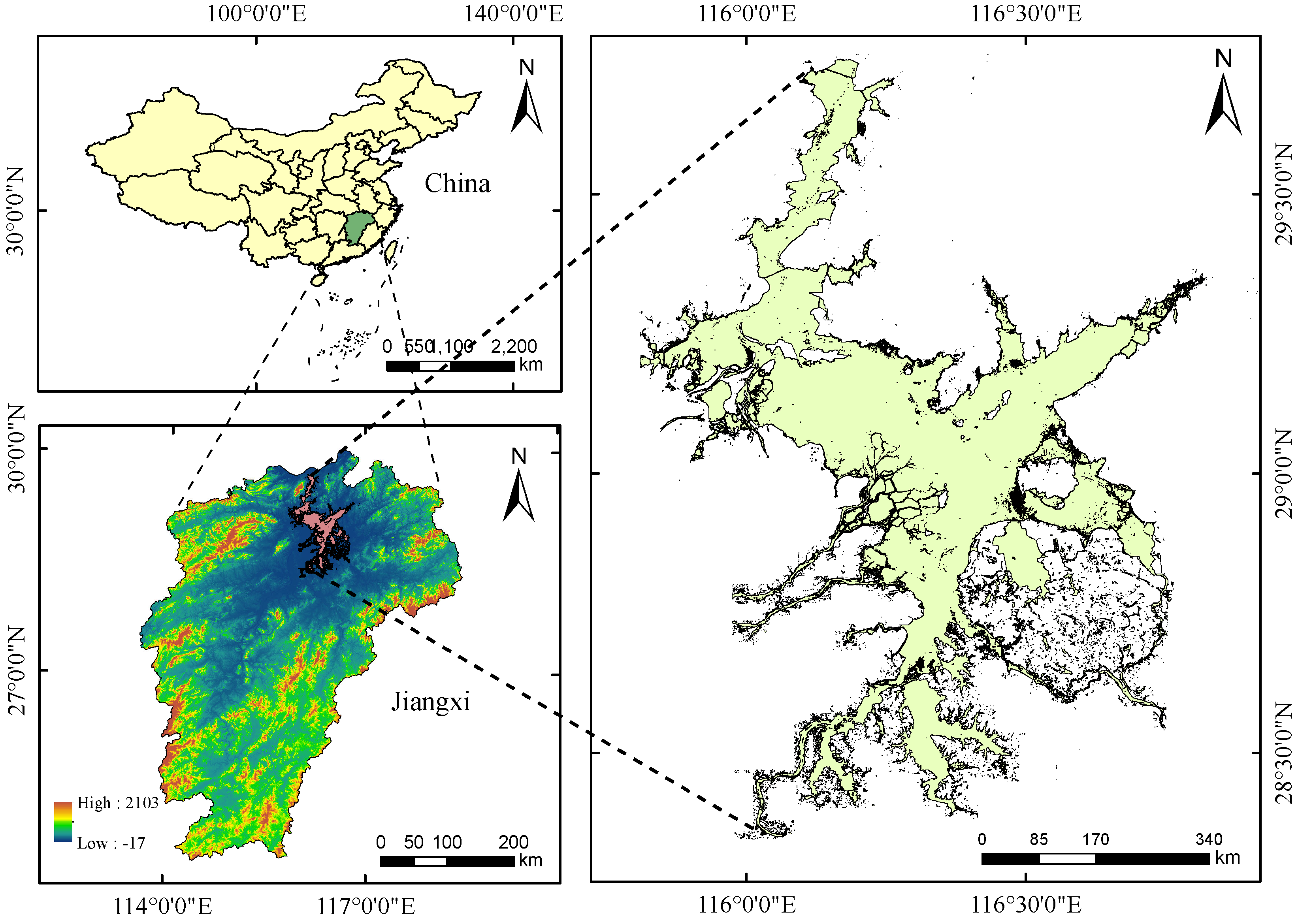
This study proposes a multi-model integrated learning method aimed at estimating the content of four water quality parameters (Chl-a, TP, TN and COD) in Poyang Lake. Specifically, the main steps are: (1) The preprocessing of Sentinel-2 product remote sensing images. (2) The selection of related bands and related indices. (3) The matching of water quality parameter data with the reflectance of Sentinel-2 products. (4) The application of the evaluation model to estimate the water quality parameters from 2017 to 2018. The workflow adopted is shown in Figure 1.

2.1. Study Area

Poyang Lake (${28}^{\circ }{22}^{\prime }$–${29}^{\circ }{45}^{\prime }$ N, ${115}^{\circ }{47}^{\prime }$–${116}^{\circ }{45}^{\prime }$ E) is located in the north of Jiangxi Province, spanning three cities of Jiujiang, Nanchang and Shangrao. It is the largest freshwater lake in China and the second largest lake in China, as shown in Figure 2. The Poyang Lake basin is an important grain production area and fishery base in China [41]. Poyang Lake is 173 km long from north to south, 74 km wide at its widest point from east to west, has a shoreline of 1200 km, and has a lake surface area of 3283 km² when the lake mouth water level is 21.71 km. The lake water is mainly supplied by rivers such as Ganjiang, Fuhe, Xinjiang, Raohe, Xiuhe and Boyang River, Xihe, etc., and after regulation and storage, it flows northward into the Yangtze River from the lake mouth, with an annual average inflow of 146 billion cubic meters into the Yangtze River. The Poyang Lake water system basin covers an area of 162,200 km², accounting for about 97% of the basin area of Jiangxi Province and 9% of the Yangtze River basin area. Poyang Lake plays an important role in regulating the water balance between the basin and the main stream of the Yangtze River, and in various ecological functions such as flood storage and maintaining biodiversity.

2.2. Data Processing

2.2.1. Sentinel-2 Data

This study uses images obtained from the Sentinel-2A/B satellites launched by the European Space Agency. The remote sensing images of Sentinel-2 can be downloaded for free from the Copernicus Data Center (https://scihub.copernicus.eu, (accessed on 6 July 2023)), and the parameters of Sentinel-2 are shown in

Table 1. The Sentinel-2 bands used in this study and its parameters.

Sentinel-2 Bands	Central Wavelength (nm)	Resolution (m)
Band 2 (Blue)	490	10
Band 3 (Green)	560	10
Band 4 (Red)	665	10
Band 5 (Red Edge)	705	20
Band 6 (Red Edge)	740	20
Band 7 (Red Edge)	783	20
Band 8 (NIR)	842	10
Band 8A (Narrow NIR)	865	20
Band 11 (SWIR)	1610	20
Band 12 (SWIR)	2190	20

. The Sentinel-2 mission includes two polar-orbiting satellites, Sentinel-2A and Sentinel-2B, launched on 23 July 2015, and 2 May 2017, respectively, achieving a high repeat time resolution of 3 days at the equator and 5 days at mid-latitudes [42,43]. Each satellite is equipped with a Multispectral Instrument (MSI), covering multiple spectral bands from visible light to shortwave infrared (SWIR). Sentinel-2 data provides 13 spectral bands with resolutions of 10 m, 20 m, and 60 m, capable of monitoring high-yield water bodies and other extreme conditions. Due to the cloud cover of Sentinel-2 products being greater than 10% at closely measured time points in the summer in this region, greatly affecting the use of these products, we did not evaluate the water quality parameters for the summer. This study selected Sentinel-2 Level-1C products (Top of Atmosphere (TOA) reflectance) images obtained from January to May and September to December each year from 2017 to 2018, with the cloud cover of each image block being less than 10%. The selected images were all atmospherically corrected using the default algorithm built into the ACOLITE software package (https://github.com/acolite, (accessed on 15 July 2023)), and batch processing was performed using Python code. Vanhellemont et al. [44] and Saberioon et al. [45] have verified the good performance of ACOLITE in inland waters. We used bilinear interpolation to upscale the low-resolution bands (20 m and 60 m) to a 10 m resolution. Then, we selected bands B2, B3, B4, B5, B6, B7, B8, B8A, B11, and B12, and used the GDAL library to complete the multi-band synthesis and image mosaicking. Finally, we obtained a full high-resolution image of Sentinel-2. Due to the high temporal and spatial resolution and rich spectral information of Sentinel-2 MS data, it is extremely beneficial for monitoring water quality changes in complex water bodies such as Poyang Lake.

2.2.2. In-Situ Data Collection

This study uses the Poyang Lake water environment monitoring dataset collected by the Poyang Lake Wetland Comprehensive Research Station of the Chinese Academy of Sciences from 2017 to 2018 [46]. This dataset includes water quality parameters (Chl-a, TP, TN and COD) for the main lake area in January, April, July and October each year. To ensure year-round water sampling, regular monitoring points are set up in the main lake area that has water all year round. During the measurement process, we use YSI’s EXO multi-parameter water quality meter to measure the concentration of Chl-a, a UV spectrophotometer to determine the content of TP and TN, and a titration method to determine COD.

Table 2. Sampling dates and mean values of sampling data for the study area.

Date (YY-MM)	Chl-a (mg/m3)	TP (mg/L)	TN (mg/L)	COD (mg/L)
2017-1	1.03	0.12	2.06	*
2017-4	3.98	0.14	1.91	*
2017-10	3.53	0.08	1.97	2.79
2018-1	3.95	0.13	2.98	3.47
2018-4	5.19	0.16	2.37	2.58
2018-10	6.27	0.12	1.89	2.30

* TIndicator not monitored at representative monitoring sites.

shows the average values of these four parameters. Through long-term observation of regular monitoring points, we reveal the seasonal and interannual variation patterns of Poyang Lake’s water quality in recent years. These data provide an important reference for us to monitor and protect the water quality of Poyang Lake.

2.2.3. Explanatory Variables

Considering that we have only spectral bands as input variables cannot fully mine the potential relationships among the data, we adopt related indices used in previous water body monitoring, such as NDCI [47]. These indices have been verified for their feasibility, thus avoiding redundant work of band combinations. Therefore, in this study, we selected 15 variables, including 10 spectral bands and 5 related indices, as shown in

Table 3. Explanatory variables considered in this experiment.

Variable	Resolution (m)	Description
B2	10	Visible blue
B3	10	Visible green
B4	10	Visible red
B5	10	Near-infrared
B6	10	Near-infrared
B7	10	Near-infrared
B8	10	Near-infrared
B8A	10	Near-infrared
B11	10	Shortwave infrared
B12	10	Shortwave infrared
Enhanced Three	10	B6 − B5
NDCI	10	(B5 − B4)/(B5 + B4)
$T{P}_{index}$	10	B2/(B3 + B4 + B12)
$T{N}_{index}$	10	(B11 − B12)/(B5 + B8A)
$CO{D}_{index}$	10	(B6 + B8A)/(B4 − B12)

. The spectral indices are composed of the surface reflectance values of bands B2, B3, B4, B5, B6, B7, B8, B8A, B11, and B12, and we chose the band combinations used in existing algorithms for the related indices. When evaluating the content of Chl-a, we use 10 bands and NDCI, Enhanced Three [48] as input variables, similarly, when evaluating the content of other water quality parameters, we choose 10 bands and related indices as input variables, including $T{P}_{index}$, $T{N}_{index}$ and $CO{D}_{index}$ [31]. The spatial resolution of all explanatory variables is uniformly 10 m to ensure the consistency and accuracy of the data.

2.3. Correlation Analysis

Correlation analysis is an analysis of the relationship between two or more variables, often used to measure the degree of association between variables. To demonstrate the independence of water quality concentration measurement data, this study uses the Pearson correlation coefficient. The correlation coefficient, a normalized measure of the covariance and standard deviation between two variables, quantifies their degree of correlation. This is calculated as per Equation (1). Its value lies between −1 and +1, with a larger absolute value indicating a stronger correlation.

$$r(x,y)=\frac{{\sum }_{i=1}^n(x_i-\overline{x})(y_b-\overline{y})}{\sqrt{{\sum }_{i-1}^n{(x_i-\overline{x})}^2{\sum }_{i-1}^n{(y_i-\overline{y})}^2}}$$

(1)

$r(x,y)$ represents the correlation coefficient between water quality parameters, $x_i$ and $y_i$ represent the sample values of the water quality parameters, and $\overline{x}$ and $\overline{y}$ represent the average values of the sample variables. The closer $r(x,y)$ is to 1, the stronger the correlation between the variables.

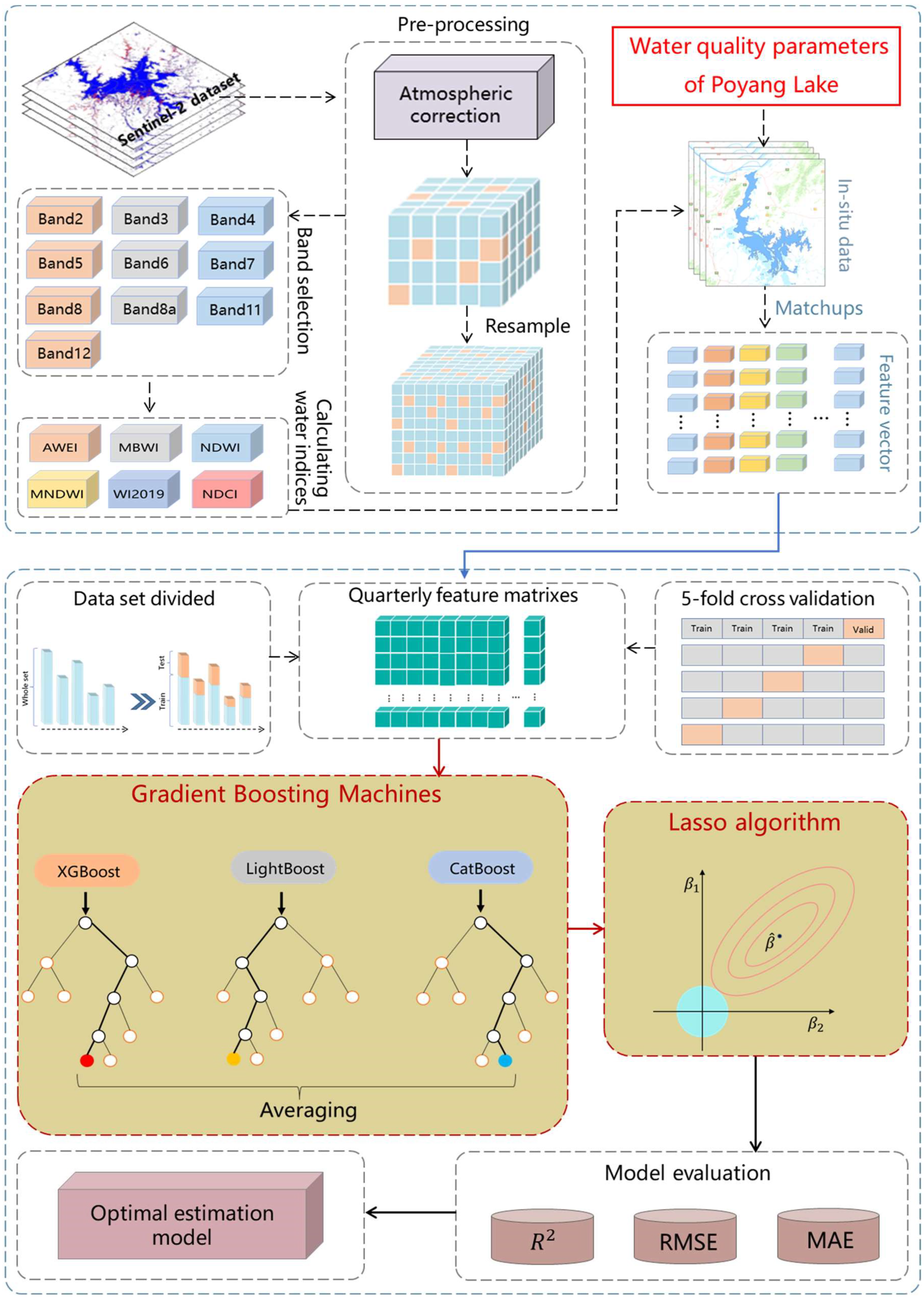
2.4. Model Development

In this study, we developed a multi-model integrated learning method, named STE. This method uses an integrated learning framework, first introducing the Gradient Boosting Machine (GBM) to acquire input data and generate independent prediction results. Different machine learning models have different perceptual abilities and can extract different features from the data. Numerous studies have shown that averaging over ensemble members using multiple models can yield more accurate and reliable predictions than a single model [49]. Finally, the Lasso algorithm is introduced as a combination method to form ensemble predictions, thereby maximizing robustness and minimizing the possibility of overfitting. In this study, based on the characteristics of the data used, we chose three Boosting algorithms as the basic regression models, taking the B2, B3, B4, B5, B6, B7, B8, B8A, B11, and B12 bands of Sentinel-2 and five related indices as the input variables for the regression model. The related indices as input variables can fully mine the potential relationships among the data, further ensuring the accuracy of the model. The specifics are as follows.

2.4.1. Ensemble Model

An ensemble model is a powerful machine learning method that can prevent overfitting and improve generalization ability [50]. This model is essentially built from multiple weakly supervised learning models, and then optimized the final prediction results through methods such as averaging. This method can reduce the accuracy bias of individual models, thereby improving the robustness and reliability of the overall model.

In ensemble learning, it is usually recommended to use heterogeneous base learners, because this can increase the diversity between models and thus improve the generalization effect [51]. In the field of machine learning, there are many different types of models, each model has a unique data perception ability, and is committed to extracting different types of features from the data. Therefore, by combining different machine learning models, we can better understand and perceive data, thereby improving the performance of the overall model [52].

2.4.2. Gradient Boosting Machine

GBM is a machine learning technique that consists of multiple weak prediction models (usually decision trees). In each iteration, it trains a new weak prediction model to fit the prediction error of all previous models (i.e., the difference between the true value and the predicted value), and then adds the prediction result of this new model to the previous total prediction result, thus obtaining a more accurate and stable prediction model. Currently, there are three GBM algorithms that are widely praised in the machine learning field, namely XGBoost, LightGBM, and CatBoost.

XGBoost is an efficient boosting algorithm that can be used to solve prediction and classification problems based on the gradient boosting framework. The classification and regression trees (CART) in XGBoost are sequentially constructed, and each new tree will correct the prediction error of the previous trees, making the model able to handle highly correlated features and reduce the problem of multicollinearity [53]. XGBoost also controls the complexity of the tree and prevents overfitting by adding regularization terms to the objective function. Therefore, XGBoost algorithm has the advantages of the fast execution and integration of high-dimensional feature processing.

LightGBM, an advanced ensemble learning algorithm, is built upon the gradient boosting decision tree (GBDT), a type of boosting algorithm. It primarily employs two novel techniques, gradient-based one-side sampling (GOSS) and exclusive feature bundling (EFB), to enhance both training efficiency and accuracy. GOSS, in particular, selects samples with larger gradients from the dataset, thereby amplifying their contribution to information gain. EFB combines some features with low correlation into a group to reduce data dimensionality [36]. This makes LightGBM superior to other boosting algorithms in terms of training speed and prediction performance [54,55,56].

CatBoost is a GBDT based on machine learning algorithm. Its uniqueness lies in its ability to handle heterogeneous features, noisy data, and complex dependencies. This algorithm employs a method based on objective statistics aimed at reducing computational complexity and uses Bayesian optimization to avoid the risk of overfitting. In the process of model construction, CatBoost uses a greedy search strategy, progressively integrating weak models to build a powerful predictive model [57]. Simultaneously, CatBoost introduces an ordered boosting method to change the gradient estimation method in classical algorithms. This method can effectively overcome the prediction offset caused by gradient bias, thereby further enhancing the generalization ability of the model [40].

2.4.3. The Least Absolute Shrinkage and Selection Operator

The Lasso algorithm [58] is an optimized least squares estimation method. It introduces a tuning parameter Lambda ($\lambda$) to penalize the regression coefficients, thereby achieving the minimization of the sum of squared errors. Specifically, the LASSO algorithm adds a regularization term to the loss function L of multiple linear regression. This regularization term is the product of the L1 norm $\beta$ of the weight vector and the regularization coefficient $\lambda$:

$$L={∥y-X\beta ∥}^2+\lambda {∥\beta ∥}_1$$

(2)

Here, $X=(x_1,x_2,\dots ,x_k)$ represents the independent predictions of K sub-models, and y represents the true value. By introducing the L1 penalty term, we can bring sparsity into the optimal coefficients. As the value of $\lambda$ increases, the least squares estimate will be compressed to 0, and large estimates will be compressed to a constant. In this study, we use a grid search method to determine the optimal $\lambda$ value between 0.001 and 1.

2.5. Regression Evaluation Metrics

To evaluate the performance of the model, we adopted the coefficient of determination ($R^2$), root mean squared error (RMSE) and mean absolute error (MAE) as the evaluation indicators. RMSE is an indicator that reflects the average error size between the predicted values and the actual values. RMSE is commonly used to evaluate the fitting effect of regression or compare the advantages and disadvantages of different models. It is considered as an excellent general error indicator for numerical prediction. MAE is an indicator that measures the average deviation degree between the predicted values and the actual values. The smaller the value, the smaller the deviation between the predicted values and the actual values, and the better the model performance. These indicators can quantitatively reflect the fitting degree and prediction accuracy of the model. Their calculation formulas are as follows:

$$R^2=1-\frac{{\sum }_{i=1}^N{\left[p_i-\widehat{p_i}\right]}^2}{{\sum }_{i=1}^n{\left[p_i-\overline{p_i}\right]}^2}$$

(3)

$$\mathrm{RMSE}={\left[\frac{1}{N}\sum _{i=1}^N{\left(p_i-\widehat{p_i}\right)}^2\right]}^{1/2}$$

(4)

$$\mathrm{MAE}=\frac{1}{N}\sum _{i=1}^N\left|p_i-\widehat{p_i}\right|$$

(5)

$p_i$ and $\widehat{p_i}$ represent the observed and model-estimated concentrations of water quality parameters for sample i, N represents the total number of observations, and $\overline{p_i}$ represents the mean of the observed values.

3. Result and Analysis

3.1. Correlation Analysis

In order to study the correlation among the water quality parameters of Poyang Lake, we calculated the correlation between each water quality parameter. As depicted in

Table 4. Correlation coefficients between water quality parameters.

	Chl-a	TP	TN	COD
Chl-a	1	0.082 *	0.294 **	0.01
TP	0.082 *	1	0.553 **	0.123
TN	0.294 **	0.533 **	1	0.184
COD	0.01	0.123	0.184	1

**, * represent 5% and 10% significance levels, respectively.

, there is a positive correlation (r = 0.533) between TP and TN. A weak correlation (r = 0.294) exists between Chl-a and TN, while the correlations among other water quality parameters are relatively weak. Based on the strength of the correlation, it can be inferred that the water quality of Poyang Lake is influenced by various parameters to some extent, leading to its spatiotemporal variation.

3.2. Model Performances and Evaluation

This study uses on-site measurement data and the reflectance of Sentinel-2 to develop a model for assessing the content of Chl-a, TP, TN and COD in Poyang Lake. We conducted a spatial correlation analysis of the four water quality parameters under investigation using ArcGIS software. The Moran’s I for Chl-a was 0.30, with a Z-score of 1.15. For TP, the Moran’s I was 0.031, with a Z-score of 0.67. TN had a Moran’s I of 0.01 and a Z-score of 0.64. Lastly, the COD had a Moran’s I of 0.32 and a Z-score of 1.11. These results suggest that all four water quality parameters are in a random state, indicating that they are not influenced by spatial autocorrelation. We selected bands B2, B3, B4, B5, B6, B7, B8, B8A, B11, and B12, as well as five related indices based on empirical algorithms already used in inland lakes, as input variables, and the concentrations of Chl-a, TP, TN, and COD as output variables. We matched the in-situ water quality data with the Sentinel-2 images (two-day window). In order to obtain a stable and reliable inversion model, it is necessary to establish a training set and a validation set before inverting the water quality parameter model. In this experiment, 80% of the total sample size of each water quality parameter (the total sample sizes of chl-a, TP, TN, and COD are 115, 210, 210, and 95, respectively) is randomly selected as the training set, and 20% as the validation set. The training set data is used to construct the inversion model, using relevant bands and indicators as input factors. The validation set is used to verify the accuracy of the model. This is part of our research, aiming to accurately assess the water quality of Poyang Lake through scientific methods.

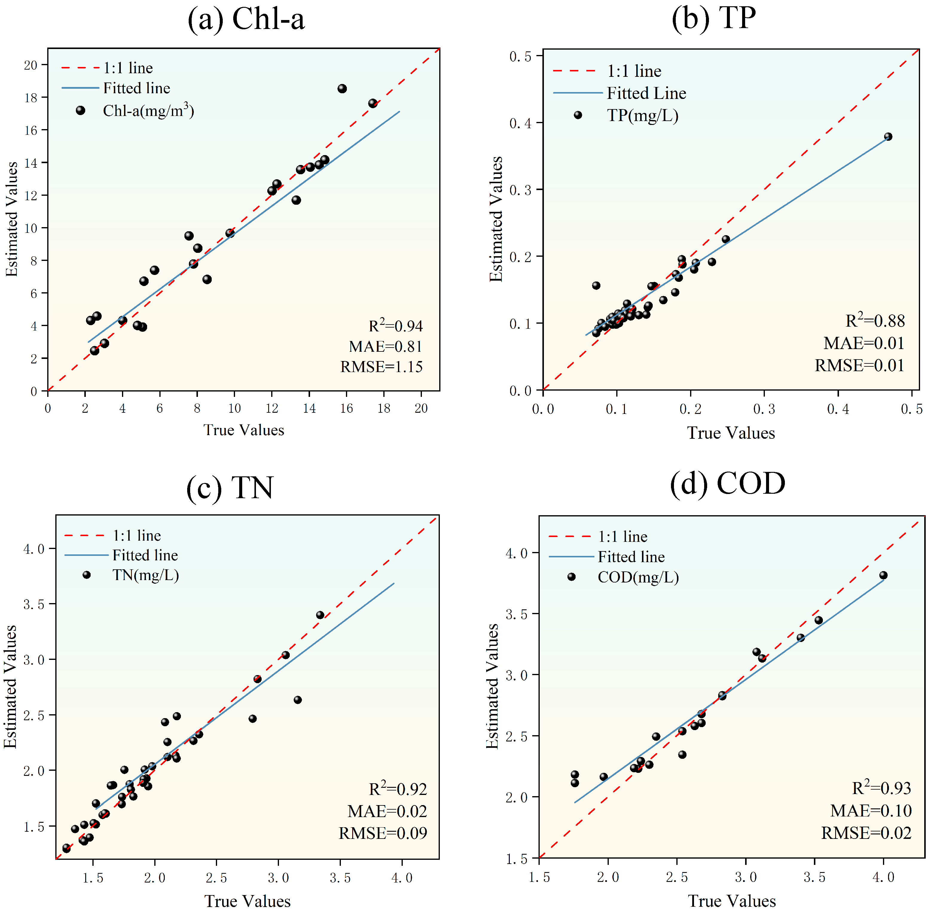
3.2.1. The Performance of The STE Model

Figure 3 shows the performance of the STE model, and we find that the model performs well on the test data. Overall, the estimation and field measurement of Chl-a concentration have high consistency. The $R^2$ for all water quality parameters are greater than 0.85, indicating that this model has strong data mining capabilities, indicating that the model has strong data mining ability. Among the three water quality parameters, Chl-a has the highest prediction accuracy ($R^2$ = 0.94, RMSE = 1.15 mg/m³, and MAE = 0.81 mg/m³), and TP has the lowest prediction accuracy ($R^2$ = 0.88, RMSE = 0.01 mg/L, and MAE = 0.01 mg/L). The performance of the evaluation model is influenced by the concentration of water quality parameters. In this dataset, the concentration of TP is relatively low, resulting in the lowest prediction accuracy for TP. By comparison, we find that all the machine learning methods used in this study have superior data mining ability, among which GBM has the most significant data mining ability. Then, after further improving the prediction accuracy of the model by Lasso algorithm, it proves the effectiveness of the multi-model ensemble strategy proposed in this paper.

3.2.2. Comparison with Other Models

We compared the performance of our proposed STE model with five commonly used machine learning methods (XGBoost, CatBoost, LightGBM, RF, and SVR) in estimating four water quality parameters. The evaluation indicators of each model are shown in

Table 5. Comparison of model performance metrics ($R^2$, RMSE and MAE) between STE model and other models.

Parameters	Metrics	Model
		STE	XGBoost	CatBoost	LightGBM	RF	SVR
Chl-a	$R^2$	$\mathbf{0.94}$	$0.92$	$0.92$	$0.91$	$0.78$	$0.61$
	$RMSE$	$\mathbf{1.15}$	$0.66$	$1.52$	$1.30$	$5.85$	$10.86$
	$MAE$	$\mathbf{0.81}$	$0.66$	$0.99$	$0.73$	$1.78$	$2.14$
TP	$R^2$	$\mathbf{0.88}$	$0.66$	$0.75$	$0.70$	$0.70$	$0.65$
	RMSE	$\mathbf{0.01}$	$0.02$	$0.02$	$0.02$	$0.03$	$0.05$
	MAE	$\mathbf{0.01}$	$0.03$	$0.02$	$0.02$	$0.10$	$0.12$
TN	$R^2$	$\mathbf{0.92}$	$0.88$	$0.87$	$0.85$	$0.80$	$0.63$
	RMSE	$\mathbf{0.02}$	$0.04$	$0.05$	$0.03$	$0.05$	$0.09$
	MAE	$\mathbf{0.09}$	$0.12$	$0.14$	$0.12$	$0.17$	$0.17$
COD	$R^2$	$\mathbf{0.93}$	$0.92$	$0.90$	$0.74$	$0.82$	$0.69$
	RMSE	$\mathbf{0.02}$	$0.04$	$0.04$	$0.03$	$0.07$	$0.11$
	MAE	$\mathbf{0.10}$	$0.13$	$0.14$	$0.12$	$0.21$	$0.15$

For each water quality parameter, the evaluation metrics with higher performance are shown in bold.

. However, these models rely on data from certain specific research areas and may not perform well in other areas. In the evaluation model, the concentration of water quality parameters has an impact, with the concentration of TP being relatively low. At the same time, TP is a non-optically active parameter, and a single machine learning algorithm cannot fully exploit its nonlinear relationship with surface reflectance. The STE model studied in this paper performs better on the test set. Although the bands from different satellites may have some impact, the input variables of this model include multiple water body indices. These indices can reflect the optical properties and water quality conditions of the water body, thereby enhancing the correlation between data and overall model performance stability. In addition, we found that all models estimate Chl-a quite accurately, while estimating TP is the most difficult. Except for the fitted STE model, $R^2$ greater than 0.85, and $R^2$ of other models are all less than 0.8. The STE model proposed in this paper significantly outperforms other models in evaluation indicators such as $R^2$, RMSE, and MAE, indicating that it has strong potential and application value in estimating water quality parameters.

3.3. Spatial and Temporal Distribution of Water Quality Parameters

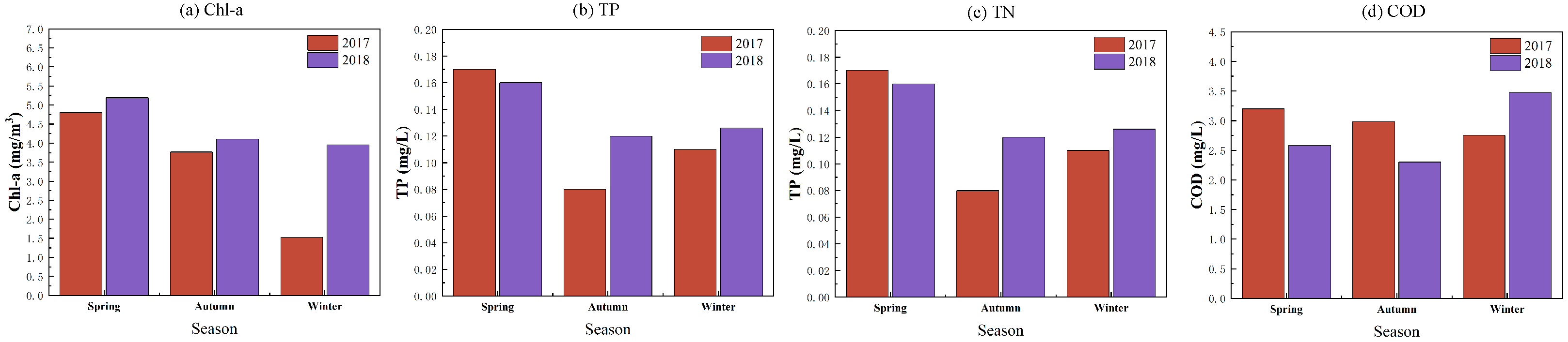
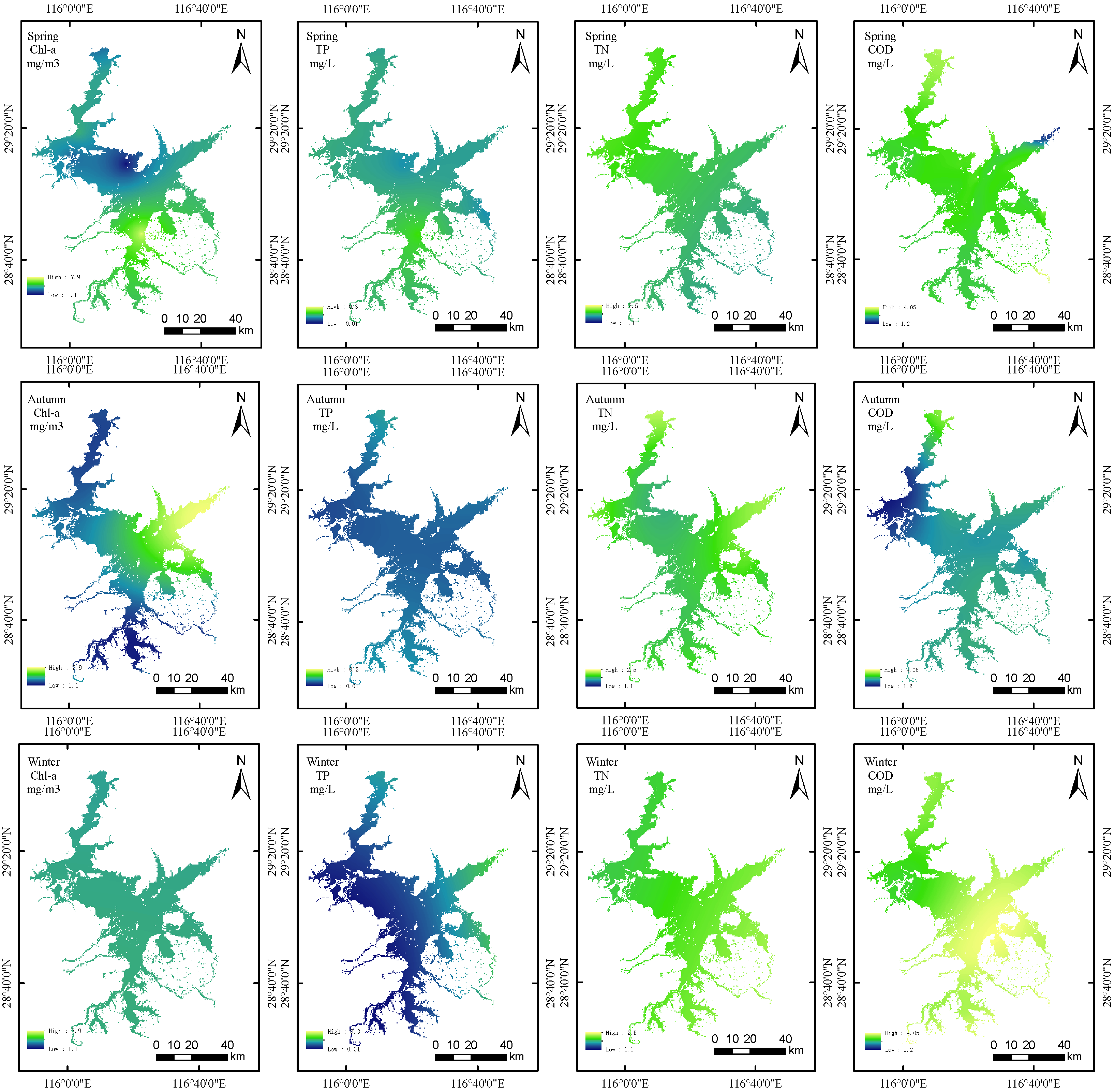
3.3.1. Seasonal Variation of Four Water Quality Parameters

To observe the seasonal distribution of Chl-a, TP, TN, and COD in Poyang Lake, the model proposed in this paper is used to retrieve the concentration of each parameter in the water based on sampling points and Sentinel-2 images. The date of the Sentinel-2 images used is close to the date of in situ sampling point measurements. Figure 4 shows the average concentrations of Chl-a, TP, TN, and COD corresponding to the inversion results for each season from 2017 to 2018. As depicted in Figure 5, we have charted the seasonal distribution of various water quality parameters. As can be seen from the figure, the seasonal variation of Chl-a is the most significant, reaching its peak in spring, followed by autumn, and lowest in winter. This may be related to the increase in water temperature and light intensity in spring, which is conducive to the reproduction of algae such as cyanobacteria. The massive growth of cyanobacteria in summer also results in a higher concentration of Chl-a in autumn. Conversely, the TP concentration is at its maximum in spring and minimum in autumn and winter. This could be due to local temperature and precipitation changes, causing phosphorus elements from soil and vegetation to be swept into the water body with the springtime increase in temperature and rainfall. The TN concentration does not change significantly throughout the year, but it is slightly higher than other seasons in winter. The main reason may be that there is less rainfall in winter, while nitrogen elements from domestic pollutants around the watershed flow into the lake. The COD does not change much in spring and winter, and the concentration is high, while the concentration is low in autumn. The frequency and intensity of summer rainfall lead to an influx of nutrients like nitrogen and phosphorus into the reservoir, thereby causing a rise in the concentration of Chl-a.

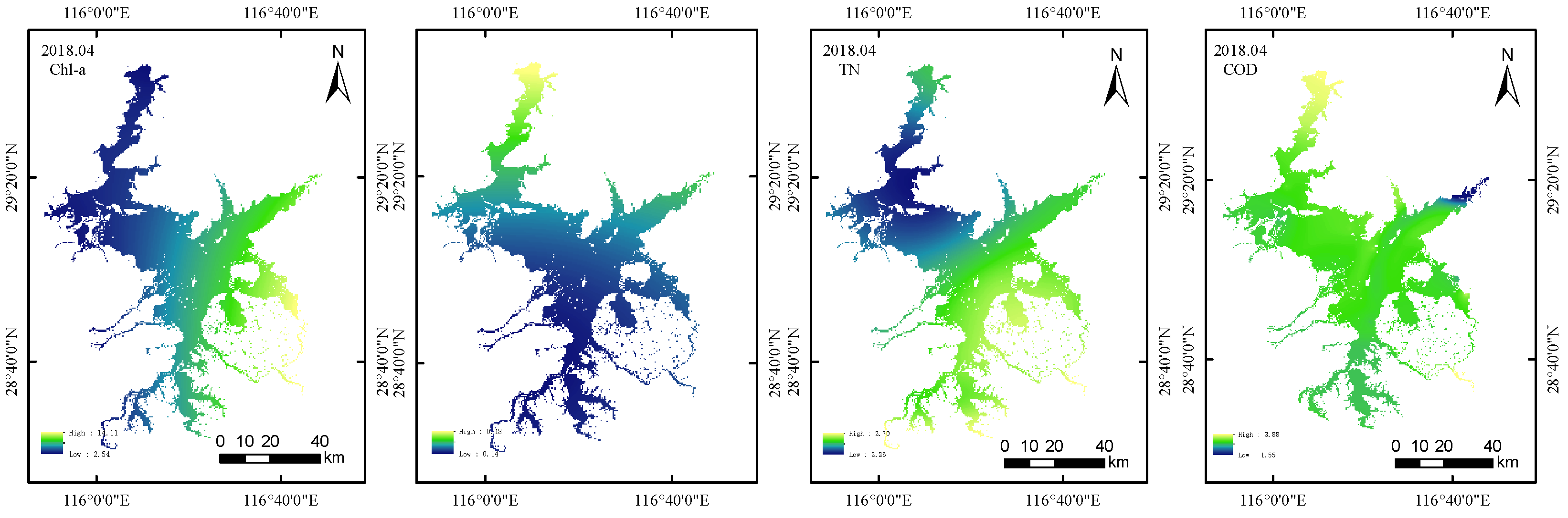
3.3.2. Spatial Variation of Four Water Quality Parameters

To further validate the model’s applicability from this study, we utilized it for the remote sensing image analysis of Poyang Lake. As depicted in Figure 6, the spatial distribution of Chl-a, TP, TN, and COD in Poyang Lake is shown. The figure reveals that the majority of the water areas in the study region are in a healthy condition, aligning with the findings from the 2018 Water Resources Bulletin of Jiangxi Province. The Chl-a and TN contents in the lake tail are higher than those in the lake center and lake head, which may be related to the influence of exogenous pollutant input and water retention from upstream in the lake tail. The elevated concentrations of Chl-a and TN in the lake’s center could be attributed to the lake’s predominantly sloping terrain. Frequent rainfall can lead to soil erosion, introducing nitrogen and phosphorus elements into the lake’s center. The relatively high TP concentration at the lake’s head might be associated with the widespread presence of industrial parks and heightened human activity in that area. A large amount of nutrients from urbanization and industrialization flow into the lake head, resulting in high TP concentration.

4. Discussion

In this study, we resampled Sentinel-2 images to enhance their spatial resolution to 10 m. This is because in the spectral indices and inversion models we constructed, the initial resolution of most bands is either 10 m (e.g., bands 2, 3, 4, and 8) or 20 m (e.g., bands 5, 6, 7, 8A, 11, and 12). By resampling these coarse spatial resolution bands to a finer spatial resolution, we can enrich the spatial information. Considering the complexity of the optical environment of inland lakes and the spatial variability of water quality, in order to better retain spatial details and display the spatial variation of water quality as much as possible, we chose to resample the coarse spatial resolution bands to 10 m.

Cloud contamination is one of the main reasons limiting the application of remote sensing images. Due to the obstruction of its cloud layer, it is impossible to observe surface information. We performed cloud removal operations on Sentinel-2 remote sensing images. Cloud removal can significantly reduce the situation where the cloud layer obscures the surface, making the surface information more clearly displayed, which is particularly important for the quantitative extraction of surface features, such as the extraction of surface reflectance of water bodies in this study. At the same time, we shortened the time window for selecting images, which helps to capture the remote sensing images closest to the sampling time of water quality parameters, can reduce the variation error caused by too long time intervals, and improve the accuracy and reliability of the results.

This paper aims to enhance the accuracy and efficiency of remote sensing inversion of water quality parameters using machine learning ensemble models. The theoretical basis for the remote sensing quantitative inversion of water quality parameters is the significant difference in reflectance within a certain range due to the difference in water component content. This paper explores the potential of using various machine learning ensemble models to retrieve water quality indices (non-optical/optical active parameters). The machine learning ensemble model reflects the complex nonlinear relationship between water quality parameters and spectral reflectance. Therefore, the changes in reflectance in the study area are consistent with the changes in water quality parameter values. Typically, the process of inverting water quality parameters using satellite imagery involves analyzing the correlation between these parameters and remote sensing reflectance to construct a remote sensing inversion model. In practical research, it is common to form a robust link between point data from field sampling and surface data from remote sensing pixels of varying spatial resolutions. Both remote sensing observation values and sampling point measurement values need to be corrected based on ground reference points. The conversion of the two will inevitably produce some errors, which is a kind of uncertainty in quantitative remote sensing inversion. Therefore, we choose to use high spatial resolution images to reduce the errors brought by scale effects in the inversion process, thereby improving the accuracy and efficiency of water quality monitoring.

In addition, the proposed model still has potential room for improvement. First, the accuracy of the model highly depends on the input data. The errors in in-situ measurement data and Sentinel-2 satellite image processing may increase the uncertainty of the model, especially considering that the data we use come from different laboratories and adopt different processing methods and standards. In addition, although we have performed cloud removal operations on Sentinel-2 data to reduce the pollution of clouds and cloud shadows in the image and retain more valid information, this may introduce some errors. Therefore, when studying lake water quality assessment in the future, we must take into account this regional variability. Finally, our STE model did not incorporate spatial information and timestamps into model construction, which may affect the generalization ability of the model. Therefore, in future work, we plan to develop a reasonable spatio-temporal coding method to further improve the generalization ability of the model. This will be the focus of our attention and improvements in the next step.

5. Conclusions

In this study, we established a high-precision water quality parameter estimation model based on ensemble learning and used the 10 m high-resolution imagery of Sentinel-2 to monitor the seasonal changes of Poyang Lake from 2017 to 2018, and conducted a preliminary analysis of the spatio-temporal distribution of water quality in Poyang Lake. The conclusions of this study can be summarized as follows:

• We included multiple related indices, such as NDCI, Enhanced Three, etc., as predictors. These related indices have been used for the inversion of water quality in inland lakes, verifying their high correlation with multiple water quality parameters. These related indices can enhance the correlation between Sentinel-2 remote sensing data and water quality parameters, thereby greatly enhancing the predictive potential of the model.
• We proposed a new STE model, which combines advanced machine learning methods and uses an integrated strategy to enhance the robustness of the model. The results show that the model has good performance in achieving accurate predictions ($R^2$ > 0.85). At the same time, the water quality parameters predicted by the model are very close to the field measurement values, and can well realize the inversion of water quality parameters of medium-sized water bodies.
• We used the STE model to draw a distribution map of the seasonal and spatial changes in the study area from 2017 to 2018, and found that the water quality parameter values of Poyang Lake generally showed an upward trend and had certain seasonal changes. From the figure, it can be seen that the concentrations of Chl-a and TN at the tail of Poyang Lake are higher than those in the lake, and the TP concentration at the head of the lake is relatively high. Overall, the water quality of Poyang Lake is good, and corresponding water quality management measures should continue to be implemented.

This research offers a practical and effective approach for the surveillance and management of water quality parameters in inland water areas. Future endeavors will involve exploring the alterations in water quality parameters of inland waters based on the STE model, contributing to the safety and administration of inland water quality. Furthermore, the accuracy of the method could be improved by utilizing multiple data sources.

References

1. Duan, Z.; Bastiaanssen, W. Estimating water volume variations in lakes and reservoirs from four operational satellite altimetry databases and satellite imagery data. Remote Sens. Environ. 2013, 134, 403–416. [Google Scholar] [CrossRef]
2. Messager, M.L.; Ettinger, A.K.; Murphy-Williams, M.; Levin, P.S. Fine-scale assessment of inequities in inland flood vulnerability. Appl. Geogr. 2021, 133, 102492. [Google Scholar] [CrossRef]
3. Verpoorter, C.; Kutser, T.; Seekell, D.A.; Tranvik, L.J. A global inventory of lakes based on high-resolution satellite imagery. Geophys. Res. Lett. 2014, 41, 6396–6402. [Google Scholar] [CrossRef]
4. Yang, K.; Smith, L.C. Internally drained catchments dominate supraglacial hydrology of the southwest Greenland Ice Sheet. J. Geophys. Res. Earth Surf. 2016, 121, 1891–1910. [Google Scholar] [CrossRef]
5. Zhao, G.; Li, Y.; Zhou, L.; Gao, H. Evaporative water loss of 1.42 million global lakes. Nat. Commun. 2022, 13, 3686. [Google Scholar] [CrossRef] [PubMed]
6. Ho, J.C.; Michalak, A.M.; Pahlevan, N. Widespread global increase in intense lake phytoplankton blooms since the 1980s. Nature 2019, 574, 667–670. [Google Scholar] [CrossRef] [PubMed]
7. Zhang, S.; Yager, P.L.; Liang, C.; Shen, Z.; Xian, W. Distribution and spatial-temporal variation of organic matter along the Yangtze River-ocean continuum. Elem. Sci. Anth. 2022, 10, 00034. [Google Scholar] [CrossRef]
8. Alcântara, E.; Bernardo, N.; Rodrigues, T.; Watanabe, F. Modeling the spatio-temporal dissolved organic carbon concentration in Barra Bonita reservoir using OLI/Landsat-8 images. Model. Earth Syst. Environ. 2017, 3, 11. [Google Scholar] [CrossRef]
9. Watanabe, F.S.Y.; Alcântara, E.; Rodrigues, T.W.P.; Imai, N.N.; Barbosa, C.C.F.; Rotta, L.H.d.S. Estimation of chlorophyll-a concentration and the trophic state of the Barra Bonita hydroelectric reservoir using OLI/Landsat-8 images. Int. J. Environ. Res. Public Health 2015, 12, 10391–10417. [Google Scholar] [CrossRef] [PubMed]
10. Li, Y.; Zhang, Y.; Shi, K.; Zhou, Y.; Zhang, Y.; Liu, X.; Guo, Y. Spatiotemporal dynamics of chlorophyll-a in a large reservoir as derived from Landsat 8 OLI data: Understanding its driving and restrictive factors. Environ. Sci. Pollut. Res. 2018, 25, 1359–1374. [Google Scholar] [CrossRef] [PubMed]
11. Xiao, H.; Krauss, M.; Floehr, T.; Yan, Y.; Bahlmann, A.; Eichbaum, K.; Brinkmann, M.; Zhang, X.; Yuan, X.; Brack, W.; et al. Effect-directed analysis of aryl hydrocarbon receptor agonists in sediments from the Three Gorges Reservoir, China. Environ. Sci. Technol. 2016, 50, 11319–11328. [Google Scholar] [CrossRef] [PubMed]
12. Chawla, I.; Karthikeyan, L.; Mishra, A.K. A review of remote sensing applications for water security: Quantity, quality, and extremes. J. Hydrol. 2020, 585, 124826. [Google Scholar] [CrossRef]
13. Wang, J.; Song, C.; Reager, J.T.; Yao, F.; Famiglietti, J.S.; Sheng, Y.; MacDonald, G.M.; Brun, F.; Schmied, H.M.; Marston, R.A.; et al. Recent global decline in endorheic basin water storages. Nat. Geosci. 2018, 11, 926–932. [Google Scholar] [CrossRef] [PubMed]
14. Guo, S.; Sun, B.; Zhang, H.K.; Liu, J.; Chen, J.; Wang, J.; Jiang, X.; Yang, Y. MODIS ocean color product downscaling via spatio-temporal fusion and regression: The case of chlorophyll-a in coastal waters. Int. J. Appl. Earth Obs. Geoinf. 2018, 73, 340–361. [Google Scholar] [CrossRef]
15. He, J.; Chen, Y.; Wu, J.; Stow, D.A.; Christakos, G. Space-time chlorophyll-a retrieval in optically complex waters that accounts for remote sensing and modeling uncertainties and improves remote estimation accuracy. Water Res. 2020, 171, 115403. [Google Scholar] [CrossRef] [PubMed]
16. Tran, T.V.; Tran, D.X.; Myint, S.W.; Huang, C.Y.; Pham, H.V.; Luu, T.H.; Vo, T.M. Examining spatiotemporal salinity dynamics in the Mekong River Delta using Landsat time series imagery and a spatial regression approach. Sci. Total Environ. 2019, 687, 1087–1097. [Google Scholar] [CrossRef] [PubMed]
17. Feng, Q.; Cheng, X.; Shen, X.; Xiao, X.; Wang, L.; Zhang, W. Inland Riverine Turbidity Estimation for Hanjiang River with Landsat 8 OLI Imager. J. Wuhan Univ. (Inf. Sci. Ed.) 2017, 42, 643–647. [Google Scholar]
18. Dong, G.; Hu, Z.; Liu, X.; Fu, Y.; Zhang, W. Spatio-temporal variation of total nitrogen and ammonia nitrogen in the water source of the middle route of the South-to-North Water Diversion Project. Water 2020, 12, 2615. [Google Scholar] [CrossRef]
19. Wang, Z.; Wei, L.; He, C.; Lu, Q. Ammonia nitrogen monitoring of urban rivers with UAV-borne hyperspectral remote sensing imagery. In Proceedings of the 2021 IEEE International Geoscience and Remote Sensing Symposium IGARSS, Brussels, Belgium, 11–16 July 2021; pp. 3713–3716. [Google Scholar]
20. Barnes, B.B.; Hu, C. Dependence of satellite ocean color data products on viewing angles: A comparison between SeaWiFS, MODIS, and VIIRS. Remote Sens. Environ. 2016, 175, 120–129. [Google Scholar] [CrossRef]
21. Tellman, B.; Sullivan, J.A.; Kuhn, C.; Kettner, A.J.; Doyle, C.S.; Brakenridge, G.R.; Erickson, T.A.; Slayback, D.A. Satellite imaging reveals increased proportion of population exposed to floods. Nature 2021, 596, 80–86. [Google Scholar] [CrossRef] [PubMed]
22. Olthof, I.; Rainville, T. Dynamic surface water maps of Canada from 1984 to 2019 Landsat satellite imagery. Remote Sens. Environ. 2022, 279, 113121. [Google Scholar] [CrossRef]
23. Achmad, A.R.; Syifa, M.; Park, S.J.; Lee, C.W. Geomorphological transition research for affecting the coastal environment due to the volcanic eruption of Anak Krakatau by satellite imagery. J. Coast. Res. 2019, 90, 214–220. [Google Scholar] [CrossRef]
24. Jiang, Q. Study on the Effectiveness Evaluation Method of Satellite Remote Sensing in the Monitoring of Lake and Reservoir Water Quality: Take GF-1 Satellite as an Example; Lanzhou Jiaotong University: Lanzhou, China, 2020. [Google Scholar] [CrossRef]
25. Barrett, D.C.; Frazier, A.E. Automated method for monitoring water quality using Landsat imagery. Water 2016, 8, 257. [Google Scholar] [CrossRef]
26. Wang, S.M.; Qin, B.Q. Research progress on remote sensing monitoring of lake water quality parameters. Huan Jing Xue=Huanjing Kexue 2023, 44, 1228–1243. [Google Scholar]
27. Sagan, V.; Peterson, K.T.; Maimaitijiang, M.; Sidike, P.; Sloan, J.; Greeling, B.A.; Maalouf, S.; Adams, C. Monitoring inland water quality using remote sensing: Potential and limitations of spectral indices, bio-optical simulations, machine learning, and cloud computing. Earth-Sci. Rev. 2020, 205, 103187. [Google Scholar] [CrossRef]
28. Xiong, Y.; Ran, Y.; Zhao, S.; Zhao, H.; Tian, Q. Remotely assessing and monitoring coastal and inland water quality in China: Progress, challenges and outlook. Crit. Rev. Environ. Sci. Technol. 2020, 50, 1266–1302. [Google Scholar] [CrossRef]
29. Xiong, J.; Lin, C.; Cao, Z.; Hu, M.; Xue, K.; Chen, X.; Ma, R. Development of remote sensing algorithm for total phosphorus concentration in eutrophic lakes: Conventional or machine learning? Water Res. 2022, 215, 118213. [Google Scholar] [CrossRef]
30. Yu, X.; Yi, H.; Liu, X.; Wang, Y.; Liu, X.; Zhang, H. Remote-sensing estimation of dissolved inorganic nitrogen concentration in the Bohai Sea using band combinations derived from MODIS data. Int. J. Remote Sens. 2016, 37, 327–340. [Google Scholar] [CrossRef]
31. Cao, X.; Zhang, J.; Meng, H.; Lai, Y.; Xu, M. Remote sensing inversion of water quality parameters in the Yellow River Delta. Ecol. Indic. 2023, 155, 110914. [Google Scholar] [CrossRef]
32. Guo, H.; Huang, J.J.; Chen, B.; Guo, X.; Singh, V.P. A machine learning-based strategy for estimating non-optically active water quality parameters using Sentinel-2 imagery. Int. J. Remote Sens. 2021, 42, 1841–1866. [Google Scholar] [CrossRef]
33. Nguyen, H.Q.; Ha, N.T.; Pham, T.L. Inland harmful cyanobacterial bloom prediction in the eutrophic Tri An Reservoir using satellite band ratio and machine learning approaches. Environ. Sci. Pollut. Res. 2020, 27, 9135–9151. [Google Scholar] [CrossRef] [PubMed]
34. Guo, H.; Huang, J.J.; Zhu, X.; Wang, B.; Tian, S.; Xu, W.; Mai, Y. A generalized machine learning approach for dissolved oxygen estimation at multiple spatiotemporal scales using remote sensing. Environ. Pollut. 2021, 288, 117734. [Google Scholar] [CrossRef] [PubMed]
35. Kim, Y.W.; Kim, T.; Shin, J.; Lee, D.S.; Park, Y.S.; Kim, Y.; Cha, Y. Validity evaluation of a machine-learning model for chlorophyll a retrieval using Sentinel-2 from inland and coastal waters. Ecol. Indic. 2022, 137, 108737. [Google Scholar] [CrossRef]
36. Ke, G.; Meng, Q.; Finley, T.; Wang, T.; Chen, W.; Ma, W.; Ye, Q.; Liu, T.Y. Lightgbm: A highly efficient gradient boosting decision tree. Adv. Neural Inf. Process. Syst. 2017, 9, 3149–3157. [Google Scholar]
37. Shi, X.; Gu, L.; Jiang, T.; Zheng, X.; Dong, W.; Tao, Z. Retrieval of chlorophyll-a concentrations using Sentinel-2 MSI imagery in Lake Chagan based on assessments with machine learning models. Remote Sens. 2022, 14, 4924. [Google Scholar] [CrossRef]
38. Zhang, Y.; Shen, F.; Sun, X.; Tan, K. Marine big data-driven ensemble learning for estimating global phytoplankton group composition over two decades (1997–2020). Remote Sens. Environ. 2023, 294, 113596. [Google Scholar] [CrossRef]
39. Chen, T.; Guestrin, C. Xgboost: A scalable tree boosting system. In Proceedings of the 22nd Acm Sigkdd International Conference on Knowledge Discovery and Data Mining, San Francisco, CA, USA, 13–17 August 2016; pp. 785–794. [Google Scholar]
40. Prokhorenkova, L.; Gusev, G.; Vorobev, A.; Dorogush, A.V.; Gulin, A. CatBoost: Unbiased boosting with categorical features. Adv. Neural Inf. Process. Syst. 2018, 11, 6639–6649. [Google Scholar]
41. Song, L.; Song, C.; Luo, S.; Chen, T.; Liu, K.; Li, Y.; Jing, H.; Xu, J. Refining and densifying the water inundation area and storage estimates of Poyang Lake by integrating Sentinel-1/2 and bathymetry data. Int. J. Appl. Earth Obs. Geoinf. 2021, 105, 102601. [Google Scholar] [CrossRef]
42. Salameh, E.; Frappart, F.; Turki, I.; Laignel, B. Intertidal topography mapping using the waterline method from Sentinel-1 &-2 images: The examples of Arcachon and Veys Bays in France. ISPRS J. Photogramm. Remote Sens. 2020, 163, 98–120. [Google Scholar]
43. Yang, K.; Smith, L.C.; Sole, A.; Livingstone, S.J.; Cheng, X.; Chen, Z.; Li, M. Supraglacial rivers on the northwest Greenland Ice Sheet, Devon Ice Cap, and Barnes Ice Cap mapped using Sentinel-2 imagery. Int. J. Appl. Earth Obs. Geoinf. 2019, 78, 1–13. [Google Scholar] [CrossRef]
44. Vanhellemont, Q. Adaptation of the dark spectrum fitting atmospheric correction for aquatic applications of the Landsat and Sentinel-2 archives. Remote Sens. Environ. 2019, 225, 175–192. [Google Scholar] [CrossRef]
45. Saberioon, M.; Brom, J.; Nedbal, V.; Souček, P.; Císař, P. Chlorophyll-a and total suspended solids retrieval and mapping using Sentinel-2A and machine learning for inland waters. Ecol. Indic. 2020, 113, 106236. [Google Scholar] [CrossRef]
46. Liu, H.; Zhang, Q.; Niu, Y.; Xu, L.; Hu, Y. A Dataset of Water Environment Survey in the Poyang Lake from 2013 to 2018; Science Data Bank: Beijing, China, 2019. [Google Scholar]
47. Mishra, S.; Mishra, D.R. Normalized difference chlorophyll index: A novel model for remote estimation of chlorophyll-a concentration in turbid productive waters. Remote Sens. Environ. 2012, 117, 394–406. [Google Scholar] [CrossRef]
48. Yang, W.; Matsushita, B.; Chen, J.; Fukushima, T.; Ma, R. An enhanced three-band index for estimating chlorophyll-a in turbid case-II waters: Case studies of Lake Kasumigaura, Japan, and Lake Dianchi, China. IEEE Geosci. Remote Sens. Lett. 2010, 7, 655–659. [Google Scholar] [CrossRef]
49. Pena, M.; van den Dool, H. Consolidation of multimodel forecasts by ridge regression: Application to Pacific sea surface temperature. J. Clim. 2008, 21, 6521–6538. [Google Scholar] [CrossRef]
50. Hosseiny, B.; Mahdianpari, M.; Brisco, B.; Mohammadimanesh, F.; Salehi, B. WetNet: A spatial–temporal ensemble deep learning model for wetland classification using Sentinel-1 and Sentinel-2. IEEE Trans. Geosci. Remote Sens. 2021, 60, 3113856. [Google Scholar] [CrossRef]
51. Zhou, T.; Lu, H.; Yang, Z.; Qiu, S.; Huo, B.; Dong, Y. The ensemble deep learning model for novel COVID-19 on CT images. Appl. Soft Comput. 2021, 98, 106885. [Google Scholar] [CrossRef] [PubMed]
52. Ganaie, M.A.; Hu, M.; Malik, A.; Tanveer, M.; Suganthan, P. Ensemble deep learning: A review. Eng. Appl. Artif. Intell. 2022, 115, 105151. [Google Scholar] [CrossRef]
53. Parsa, A.B.; Movahedi, A.; Taghipour, H.; Derrible, S.; Mohammadian, A.K. Toward safer highways, application of XGBoost and SHAP for real-time accident detection and feature analysis. Accid. Anal. Prev. 2020, 136, 105405. [Google Scholar] [CrossRef] [PubMed]
54. Su, H.; Lu, X.; Chen, Z.; Zhang, H.; Lu, W.; Wu, W. Estimating coastal chlorophyll-a concentration from time-series OLCI data based on machine learning. Remote Sens. 2021, 13, 576. [Google Scholar] [CrossRef]
55. Wang, N.; Zhang, G.; Pang, W.; Ren, L.; Wang, Y. Novel monitoring method for material removal rate considering quantitative wear of abrasive belts based on LightGBM learning algorithm. Int. J. Adv. Manuf. Technol. 2021, 114, 3241–3253. [Google Scholar] [CrossRef]
56. Zhang, T.; Su, H.; Yang, X.; Yan, X. Remote sensing prediction of global subsurface thermohaline and the impact of longitude and latitude based on LightGBM. J. Remote Sens. 2020, 24, 1255–1269. [Google Scholar] [CrossRef]
57. Zhang, Y.; Zhao, Z.; Zheng, J. CatBoost: A new approach for estimating daily reference crop evapotranspiration in arid and semi-arid regions of Northern China. J. Hydrol. 2020, 588, 125087. [Google Scholar] [CrossRef]
58. Tibshirani, R. Regression selection and shrinkage via the lasso. J. R. Stat. Soc. Ser. B 1996, 58, 267–288. [Google Scholar] [CrossRef]
Figure 1. Schematic flow of the methodological approach in this study.
Sustainability 16 03355 g001
Figure 2. Location of the study area. The left-hand part shows the geographical location and the right-hand part shows the composition of the lake.
Sustainability 16 03355 g002
Figure 3. Performances of models for water quality parameters (Chl-a, TP, TN, and COD).
Sustainability 16 03355 g003
Figure 4. Average Chl-a, TP, TN, and COD concentrations retrieved by the STE model between 2017 and 2018.
Sustainability 16 03355 g004
Figure 5. Mapping of the seasonal variation distributions of Chl-a, TP, TN and COD.
Sustainability 16 03355 g005
Figure 6. Mapping of the spatial distributions of Chl-a, TP, TN and COD.
Sustainability 16 03355 g006