Abstract
Ningbo Zhoushan Port and Shanghai Port, as the top two ports in China in terms of port cargo throughput, play a crucial role in facilitating international trade and shipping. The accurate forecasting of the cargo throughput at these ports is essential for the government planning of port infrastructure and for the efficient allocation of resources by shipping enterprises. This study proposes a novel combined forecasting method for port cargo throughput, integrating the Autoregressive Integrated Moving Average (ARIMA) model with the zonotopic Kalman filter (ZKF) to address the limitations of traditional forecasting models in terms of accuracy and timeliness. First, an ARIMA model is established to perform the preliminary forecasting of the cargo throughput time series, generating a state–space representation that captures the underlying patterns in the data. Subsequently, the ZKF is applied to filter the ARIMA predictions, dynamically adjusting the forecast intervals based on the hypercube feasible set to optimize the estimation of port throughput. The results indicate that the ARIMA–ZKF combined model significantly mitigates the effects of asynchrony and lag, achieving a high prediction accuracy and robustness. This innovative approach offers an effective new method for forecasting port throughput, providing valuable practical guidance for port development and resource management.
1. Introduction
With the development of the globalized economy, China’s foreign trade activities are becoming increasingly frequent. Ports, as the gateways to foreign trade, are becoming more vital to economic development. The port cargo throughput serves as a key indicator reflecting the scale of port operations; analyzing the characteristics of port cargo throughput data and providing more accurate forecasting is of great significance for port construction. In the context of sustainable development, the port industry faces new challenges and requirements. The accurate prediction of port cargo throughput is essential for sustainable port operations. By accurately forecasting the throughput, ports can optimize resource utilization, reduce energy consumption during operations, and minimize environmental pollution. For instance, precise prediction can aid ports in allocating berths, labor, and handling equipment more efficiently, thereby avoiding over-investment or under-utilization of resources, which aligns with the principles of sustainable development. Furthermore, effective throughput forecasting enables ports to better plan for future developments, adapt to the changing global economic and environmental landscape, and contribute to the long-term stability and sustainable development of the entire port-related ecosystem.
The forecasting methodology can generally be categorized into two types: qualitative and quantitative forecasting. Qualitative forecasting methods rely on intuition and experiential judgment, inherently possessing a strong degree of subjectivity. These methods are suitable for situations where historical data are lacking or unreliable. In contrast, quantitative forecasting methods are based on statistical principles and mathematical models, aiming to objectively predict the future development of target events by analyzing the inherent patterns in the data and identifying relationships between variables.
Quantitative forecasting methods can be further divided into single models and combination models, depending on the number of forecasting models employed [1]. Single models focus on methodological approaches and primarily include time series forecasting and causal analysis methods. Time series forecasting emphasizes the patterns and trends found within historical data, constructing models by extracting sequential features from the data over time. This approach is suitable for forecasting data that are stable and exhibit certain patterns. Common time series forecasting methods include grey models [2], exponential smoothing [3], linear regression [4], Markov chain [5], Holt–Winters [6] and so on. On the other hand, causal analysis forecasting methods focus on the causal relationships between variables, incorporating factors that may influence port throughput, such as economic indicators, regional policies, and weather conditions, into the model to determine causal relationships and predict the future throughput. Common causal analysis methods include regression analyses [7], support vector machines [8], random forests [9], and neural network [10]. Causal analysis forecasting provides a more comprehensive perspective by considering the external factors related to port throughput. However, due to the numerous and complex factors that impact port throughput, both single time series methods and causal analysis forecasting methods may exhibit limitations in their predictive accuracy. Consequently, combination forecasting models have increasingly become a focal point of research [11,12,13]. This paper conducts a study on the existing issues related to time series forecasting.
The ARIMA model is renowned for its effective time series analysis capabilities, allowing it to capture linear trends and periodic variations within time series data. It performs well in predicting non-stationary port cargo throughput time series characterized by complex data patterns. However, the ARIMA model has a limited capacity to handle seasonal fluctuations. To address this limitation, the SARIMA model extends the ARIMA framework by incorporating seasonal components into time series predictions. Nevertheless, SARIMA involves a greater number of parameters, complicating the model construction and parameter tuning processes. Paper [14] utilized the ARIMA model to forecast and analyze the cargo throughput and total import and export volumes at Shanghai Port. The results indicated that the ARIMA model could effectively fit the linear characteristics of port throughput, yielding satisfactory predictive outcomes. Paper [15] developed a SARIMA model to predict the cargo throughput at Mexican ports, providing support for port construction strategies. Paper [16] analyzed actual data from Malaysian ports and found significant discrepancies between the predicted container volumes and freight amounts when using linear ARIMA and seasonal ARIMA (SARIMA) models.
However, both ARIMA and SARIMA models rely on historical data to predict future values, which introduces a degree of lag. This lag can diminish the predictive accuracy when addressing rapidly changing time series. To enhance forecasting precision, some researchers have employed filters to process autoregressive data, leveraging their noise reduction properties and utilizing iterative methods to achieve optimal data estimation.
Addressing the limitations of the ARIMA model, Paper [17] integrated the Kalman filter to compensate for the model’s shortcomings in terms of asynchronicity and lag, successfully applying it to predict oil well production. Similarly, Paper [18] adopted a comparable strategy to forecast apple yields. Paper [19] applied Kalman filtering to reduce noise in compressor flow data, enabling the ARIMA model to more accurately identify sequential features. To mitigate noise interference during the training process of the ARIMA model, Paper [20] designed a batch sequential training scheme based on the degree of noise and its impact on modeling. Their results demonstrated that the proposed spARIMA model effectively addressed the instability caused by noise. However, despite the Kalman filtering algorithm’s impressive performance in eliminating system noise and suppressing disturbances, it requires that the noise and disturbances affecting the time series conform to specific probability distributions, which poses limitations in practical applications. In contrast, the ensemble filtering algorithm confines system noise within bounded ranges and utilizes model input–output data to restrict the true state of the system within a feasible set, thereby producing predictions that are more adaptable to uncertainty in real-world noise interference.
When studying time series forecasting issues, ensemble filtering can achieve effective predictive estimation even under non-probabilistic noise conditions, leading to an optimal feasible set that includes the true predictive results. The state feasible set refers to the collection that can encapsulate the true values of the time series and can typically be described using various spatial shapes. Common methods for describing feasible sets include intervals [21], ellipsoids [22], polytopes [23], and zonotopes [24]. Each method exhibits different computational complexities and conservativeness. Among these, the fully symmetric polytope has the advantage of minimal shape constraints and diverse spatial configurations, allowing it to accurately encase the true values of the predicted states while maintaining regularity and lower conservativeness. For instance, Paper [25] designed a fully symmetric polytope to describe the state set of a system under unknown disturbances and employed auxiliary input signals to design ensemble filters for predicting system failures. Paper [26] proposed a robust recursive polytope ensemble algorithm that forecasts the remaining lifespan of linear time-varying systems with degraded components under unknown but bounded noise conditions.
Based on the above research, this paper proposes a forecasting algorithm that integrates the ARIMA and ZKF models to address the issue of monthly port cargo throughput time series prediction. The algorithm constructs state space equations based on the time series prediction expression of ARIMA model, uses fully symmetric polytope to deal with the effects of state perturbation and other external disturbances on the prediction results, and adopts recursive computation to update the prediction results in real-time at each time step, which can effectively make up for the shortcomings of non-synchronicity and lag associated with the ARIMA model, and improve the accuracy of the model prediction. This study utilizes monthly cargo throughput data from Ningbo Zhoushan Port and Shanghai Port, spanning from June 2016 to May 2024, as the research samples. Initially, preliminary predictions are conducted using the ARIMA model, which appropriately captures the data characteristics while avoiding the complexities associated with higher-order equations. Subsequently, the recursive equations of multi-cellular Kalman filtering are combined with the prediction results for further refinement. The validity of the proposed algorithm is demonstrated through comparative analysis.
2. Proposed Theories and Methods
2.1. ARIMA Model
The Autoregressive Integrated Moving Average (ARIMA) model can be used to solve the forecasting problem of non-stationary time series; the basic principle involves first transforming the non-stationary time series into a stationary series through the process of differentiation (integration, I), and then autoregressive (autoregressive, AR) processing is applied to the lagged values, and moving average (MA) processing is conducted on the error term, which reflects the discrepancy between the true values and the observed values. Those are combined to form the ARIMA model, where is the order of the autoregressive polynomial, AR; is the number of differences, I, made to turn a non-stationary time series into a stationary time series; and is the order of the moving average polynomial, MA. The expression can be formulated as below in Equation (1):
In the above equation, is the polynomial of AR; is the polynomial of MA; is the delay operator; is the number of differentials; is the difference operator of order ; is the time series; is the white noise sequence, ; indicates the parameter in AR, ; indicates the parameter in AR, , ; and indicates the length of the sequence.
The establishment of the ARIMA model requires a stationarity test on the original time series. If the series is found to be non-stationary, multiple differencing methods are employed to convert it into a stationary series until it passes the stationarity test; the range of values of the autoregressive term and the moving average term are predicted by analyzing the plots of the autocorrelation function (ACF) and partial autocorrelation function (PACF) after differencing; combined with the AIC (Akaike information criterion) information criterion, the optimal parameter combinations are screened to complete the construction of the ARIMA model. After the model is established, it is essential to test whether the residuals conform to white noise, typically using the Ljung–Box test, to confirm the validity of the model. If the residuals are white noise, this indicates that the model has adequately fitted the data; otherwise, the above steps need to be repeated to re-determine the model parameters. The ARIMA model is an extension of past patterns into the future, utilizing an established sequential training model; although it has an efficient time series impact analysis, it does exhibit certain lag and asynchronicity.
2.2. Zonotopic Kalman Filter Design
2.2.1. Background Knowledge
Firstly, we will define some of the symbols used in this paper. denotes the dimensional Euclidean space. denotes the set consisting of dimensional matrices. Given the square , the superscript denotes the transposition of the matrix, and denotes the trace of the matrix, . denotes the dimensional column vector. Given vector , is a diagonal array with diagonal values equal to and ; denotes the upper and lower bounds of the vector, ; and denotes the dimensional zero vector.
is the order of a zonotope, ; the expression is
where denotes the center of the zonotope, ; denotes the generating matrix; is a column vector; the zonotope, , is an affine transformation of the hypercube ; and denotes the sum of Minkowski.
For two given zonotopes, and , their expressions for the Minkowski sum operation are . Given a matrix, , the expression for the linear transformation of the zonotope, , is .
2.2.2. Filter Design
The set-membership filter algorithm is a method that enables effective state estimation, even when the system noise does not satisfy a specific distribution law. The zonotopic Kalman filter (ZKF) is an important method in this context. It utilizes a polytope space to encapsulate the state and noise of the system, determines a new state estimation set through the state model and prediction set, and obtains the optimal estimation of the system’s state by calculating the optimal spatial set. The principles are as follows:
Consider the following linear discrete state space equation:
where denotes the state vector; is the state transfer matrix, representing the state perturbations of the system; denotes the observation vector; and is the observation matrix. and indicate process disturbances and the measurement noise in the system, which are unknown but with upper and lower bounds.
The set of zonotopes in Equation (4), below, contains the initial state, process disturbances, and measurement noise of the linear discrete system (3):
where denotes the zonotope wrapping the initial state vector, and and denote the generating matrices of the zonotope of the wrapping process disturbance, , and observation noise, .
For system (3), the design for constructing the zonotope Kalman filter is as follows:
Assume that the estimated state at moment is known to be , then the state of the system at moment , is estimated as
where denotes the optimal gain matrix of the filter at moment .
2.3. ARIMA-ZKF Combinatorial Forecasting Model
The general steps of ARIMA-ZKF modeling are shown in Figure 1, below:
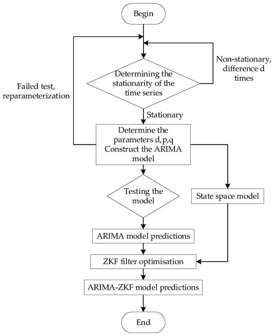
Figure 1.
ARIMA modeling process.
To combine the ZKF filtering algorithm, the key is to convert the ARIMA model into a state space model and then combine it with the ZKF filtering algorithm for the prediction. From the expansion of Equation (1), if , the port throughput at moment is
Then, the port throughput at moment can be expressed as
Set , let ; so .
The port throughput at moment can be expressed as
According to Equations (7)–(9), the state equation of the system can be obtained as
The observation equation is
The derivation, based on 1.2, leads to the predicted value of the sequence at moment :
where
For the zonotope described in Equation (4), the filter optimal gain matrix can be obtained by minimizing the Frobenius radius (F-radius) of its generating matrix to obtain the optimal state estimate. Given a symmetric positive definite matrix, , the F-radius of the zonotope can be expressed as
Let , then
When , corresponds to the minimum F-radius of the zonotope with the optimal state estimation, then the optimal gain matrix is derived as follows:
Let , then
For the prediction formula of the ARIMA model, the time series prediction result after ZKF filtering is , based on Definition 4. For the state-estimating zonotope at moment , the state vector of the system can be wrapped in a zonotope, . The upper and lower bound expressions for the time series prediction results are
3. Empirical Investigation
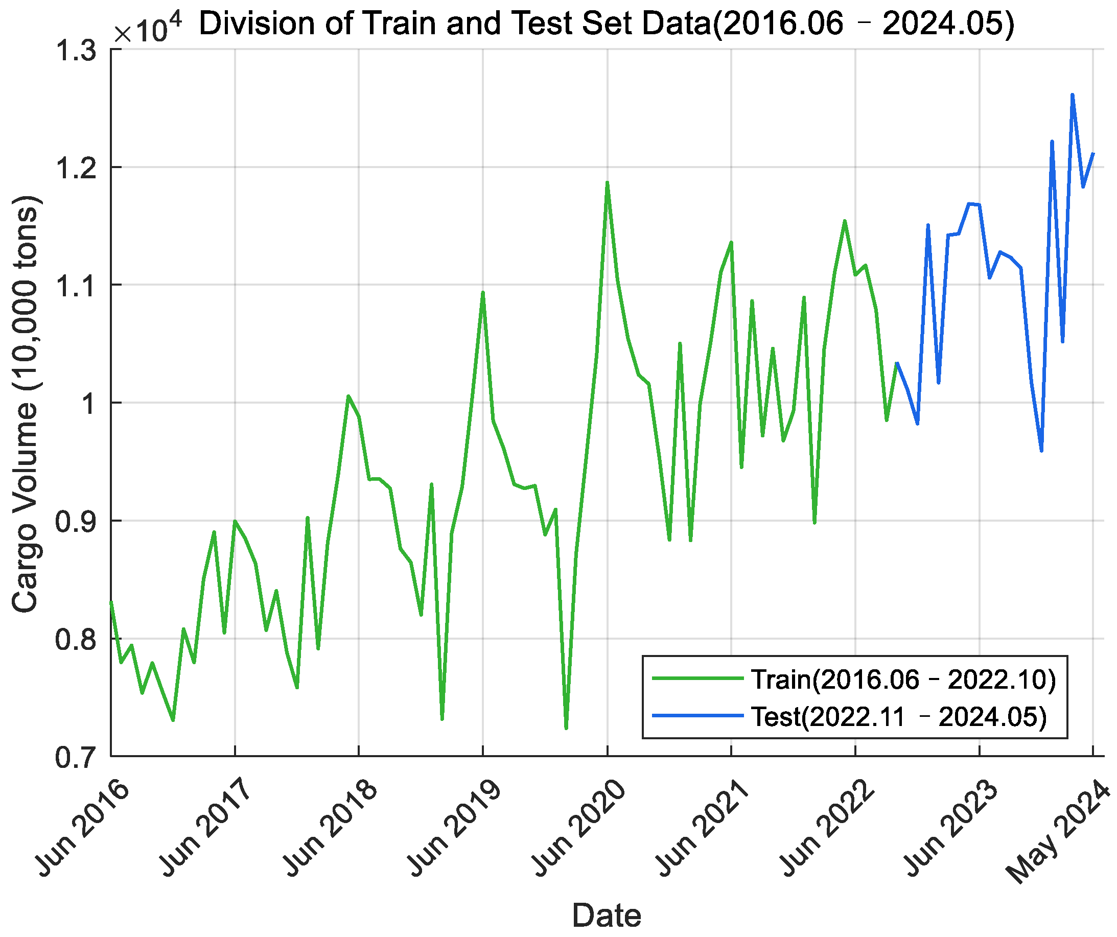
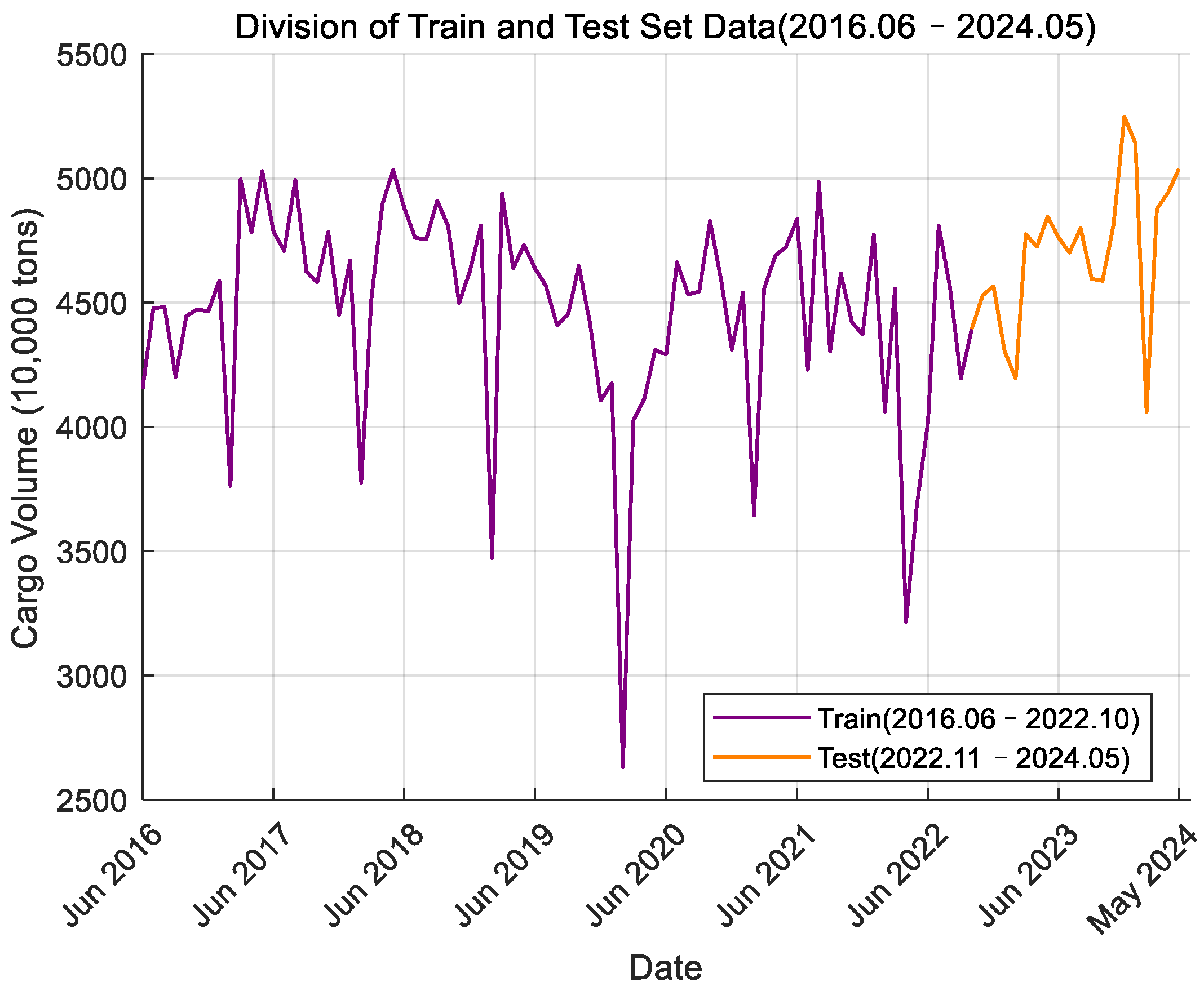
Data description: In this paper, the port cargo throughput data of Ningbo Zhoushan Port and Shanghai Port for a total of 96 months, spanning from June 2016 to May 2024, were selected, of which, the first 80% was used as the training set and the second 20% as the test set to verify the prediction effect of the model. The data came from the statistical data of the Municipal Transportation Bureau of Ningbo Municipal People’s Government and the Shanghai Municipal Bureau of Statistics.
3.1. Analysis of ARIMA Forecasting Results
The monthly port cargo throughput time series data of Ningbo Zhoushan Port and Shanghai Port from June 2016 to May 2024 were read and the time series curve was plotted. Figure 2 shows the data for Ningbo Zhoushan Port, where the green section represents the training set data and the blue section represents the test set data. Figure 3 displays the data for Shanghai Port, with the purple section indicating the training set data and the orange section indicating the test set data. From the curve graph, it can be initially determined that the time series is non-stationary. Next, the ADF (Augmented Dickey–Fuller) test will be used to verify this observation.
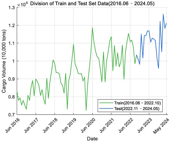
Figure 2.
Monthly cargo throughput data of Ningbo Zhoushan Port.
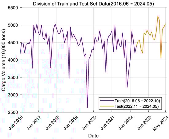
Figure 3.
Monthly cargo throughput data of Shanghai Port.
The ADF assumes that a time series is non-stationary if there is a unit root, meaning if the coefficient of the lag term in its autoregressive model is one. By calculating the ADF statistic and the corresponding p-value, it is possible to determine whether the original hypothesis of the existence of a unit root is rejected by the series, thus determining the stationary nature of the series.
For Ningbo Zhoushan Port, the results of the ADF test show that the null hypothesis (the existence of a unit root in the series) cannot be rejected with h = 0, indicating that the time series is non-stationary. Specifically, the p-value is 0.6003, which exceeds the 0.05 significance level, so the original hypothesis cannot be rejected. The test statistic is −0.13167, which is higher than the critical value of −1.9446 at the 1% level of significance. In summary, the time series is determined to be non-stationary and necessitated differencing.
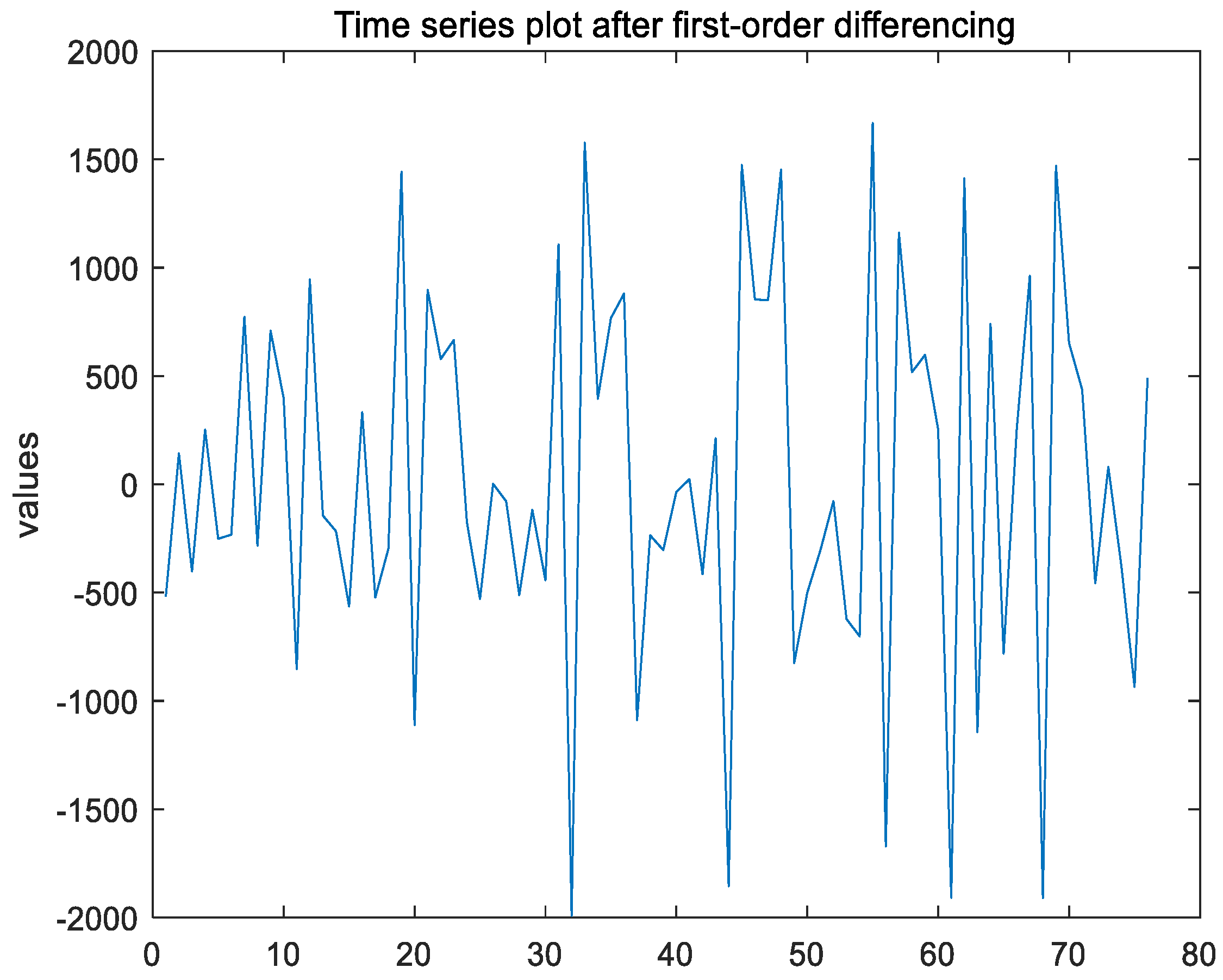
After the first-order differencing of the non-stationary time series, the ADF test result of the time series shows that h = 1, indicating that the series has been stabilized; the p-value is 0.0010, which is significantly lower than the 0.05 significance level, thereby strongly rejecting the null hypothesis; the test statistic is −13.4639, which is considerably less than the critical value of −1.9446 at the 1% significance level, which indicates that the time series has been stabilized through first-order differencing, leading to d = 1. The time series plot after first-order differencing is shown in Figure 4 below.
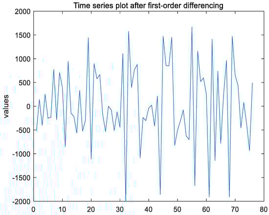
Figure 4.
Time series plot after first-order differencing of Ningbo Zhoushan Port.
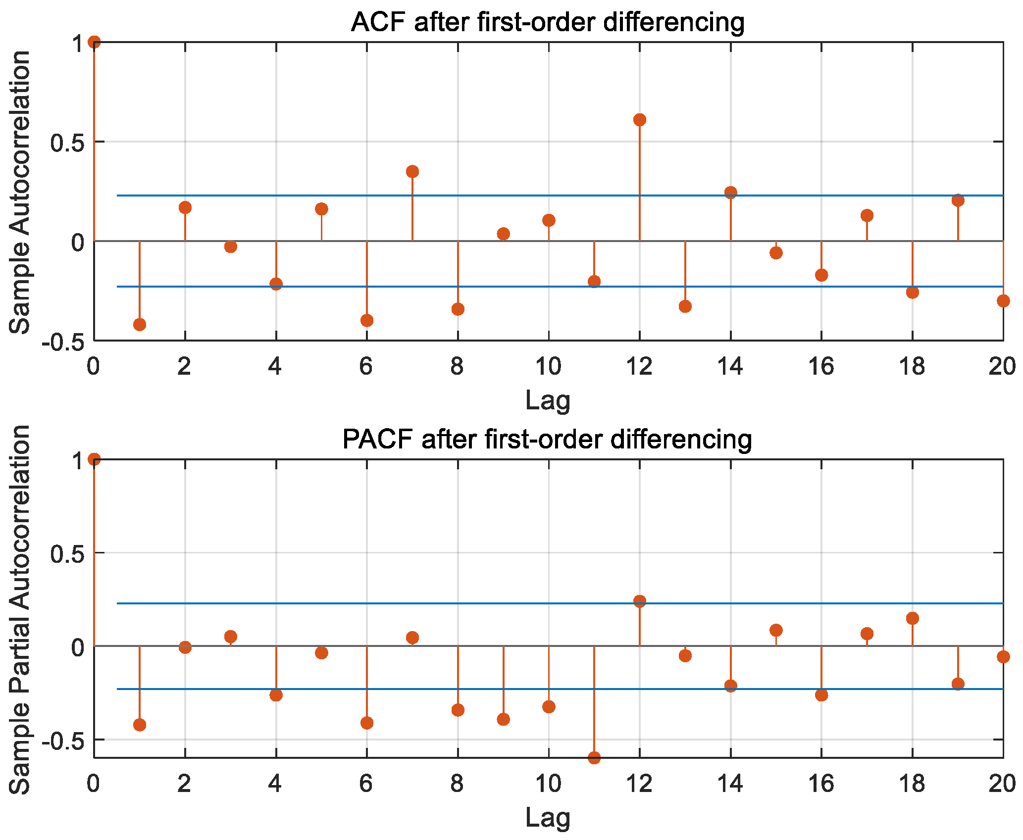
As illustrated in the ACF and PACF plots of Ningbo Zhoushan Port, after the first-order differencing of the time series in Figure 5, neither function converges to zero; instead, both exhibit a continuous and gradual decay, rather than an abrupt decline, displaying a trailing phenomenon; this behavior aligns with the characteristics expected in ARMA modeling, as shown in Table 1. Both the autocorrelation coefficient and the partial autocorrelation coefficient fall within the confidence intervals up to the second order, so the maximum order of p, and q is initially determined to be 2. The AIC criterion was used to calculate the AIC values corresponding to ARIMA models with different combinations of orders to determine the final model, as shown in Table 2 below, and the optimal ARIMA model was finally determined to be (2,1,1) by the AIC information criterion.
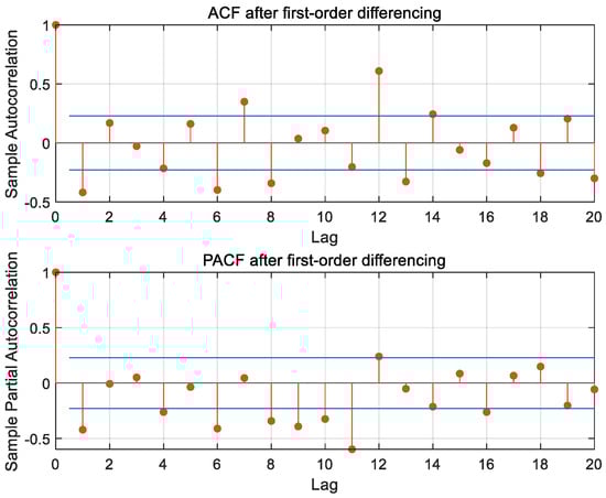
Figure 5.
ACF and PACF plot after first-order differencing of Ningbo Zhoushan Port.

Table 1.
ARIMA model identification rules.
Table 2.
AIC values corresponding to different ARIMA model parameters of Ningbo Zhoushan Port.
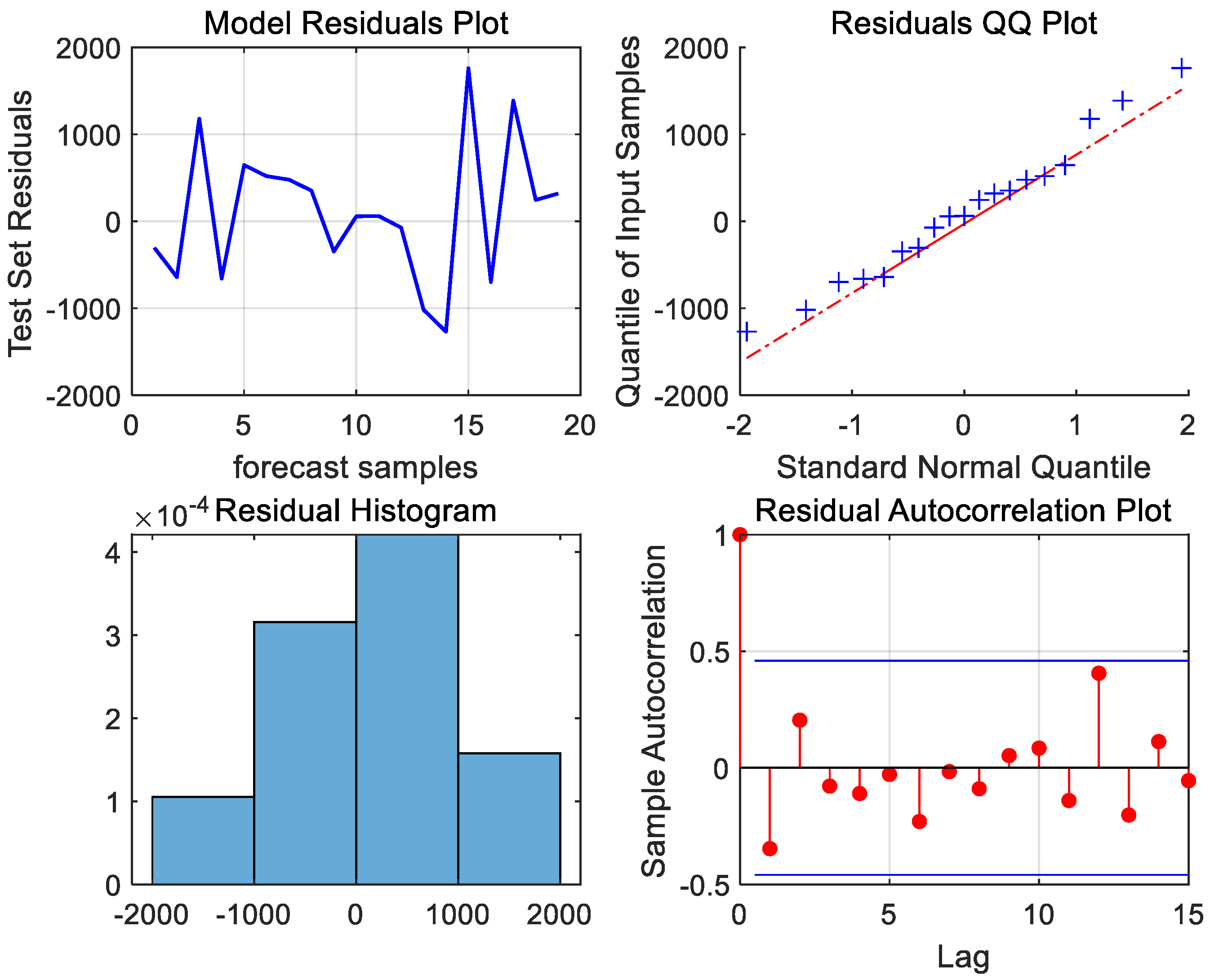
Next, the model residuals must be tested for white noise to ensure that the useful information of the port throughput time series has been adequately extracted by the developed ARIMA (2,1,1) model. From the QQ plot of the residuals and the histogram of the normal distribution of the residuals in Figure 6, it can be seen that the scatter distribution is near the fitting line, the shape of the histogram conforms to the normal distribution, the autocorrelation coefficients of the residual sequences are within the confidence intervals, and the residuals are shown to be a random sequence. To further assess the presence of white noise in the model residuals, the Ljung–Box test was conducted. The resulting p-value of 0.8582, which is greater than 0.05, confirms that the residuals are white noise sequences. This indicates that the model has successfully extracted the useful linear information, leaving only the random perturbation information that cannot be extracted by the ARIMA model.
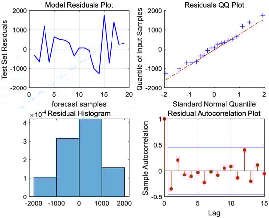
Figure 6.
Residual plot, residual QQ plot, residual histogram, and residual autocorrelation plot of Ningbo Zhoushan Port.
Similarly, we applied the above steps to establish an ARIMA model for the cargo throughput data of Shanghai Port, resulting in the final model structure of the ARIMA (2,1,1). During the ARIMA modeling process, we obtained the following parameters:
For Ningbo Zhoushan Port, ; for Shanghai Port, .
When substituting the relevant parameters of ARIMA (2,1,1) into Equation (1), represents the data from Ningbo Zhoushan Port, represents the data from Shanghai Port, and the prediction equation of the model is obtained as
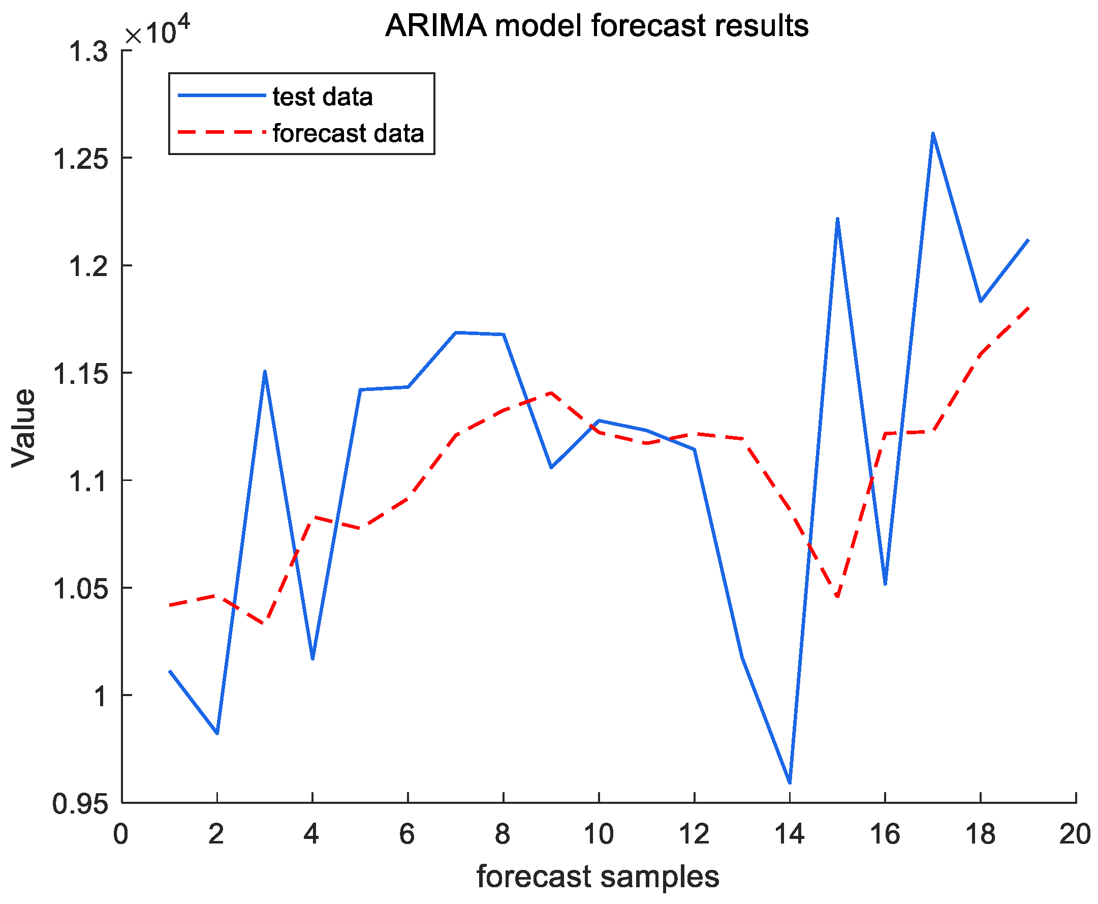
Figure 7 and Figure 8 reflect the results of the ARIMA (2,1,1) model for forecasting the cargo throughput for a total of 19 months from November 2022 to May 2024 for the test set, Ningbo Zhoushan Port and Shanghai Port. In order to evaluate the forecasting performance of the model, this study employs two commonly used metrics in time series analyses: the root mean squared error (RMSE) and the Mean Absolute Percentage Error (MAPE). The RMSE reflects the average deviation of the predicted value from the actual value, and the MAPE reflects the average level of prediction error, which is given by the following formula, where is the true value, is the observed value, and is the length of the test set.
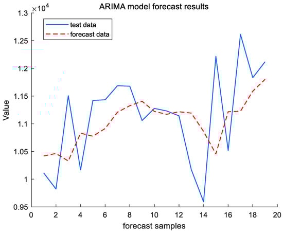
Figure 7.
ARIMA model forecast results of Ningbo Zhoushan Port.
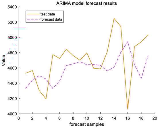
Figure 8.
ARIMA model forecast results of Shanghai Port.
For Ningbo Zhoushan Port, the RMSE = 788.8669 and the MAPE = 5.706%; for Shanghai Port, the RMSE = 344.3148 and the MAPE = 5.8658%. The prediction results indicate that the ARIMA (2,1,1) is feasible for forecasting the cargo throughput at Ningbo Zhoushan port and Shanghai Port. However, as illustrated in Figure 7 and Figure 8, while the model captures the trend of the port throughput changes, the relatively high root mean squared error (RMSE) suggests that its predictive performance is inadequate, particularly in the presence of significant data fluctuations. Consequently, the predictions may be inaccurate and exhibit lagged effects. To address these limitations, we propose further enhancements by integrating a setter filter.
3.2. ARIMA-ZKF Model Forecasting Analysis
Combining Equations (9), (11), (21) and (22) yields
The observation equation of the throughput forecasting model is
After obtaining the state space equations, the predictions were filtered and analyzed in conjunction with the set member filter, as shown in Figure 9 and Figure 10, below.
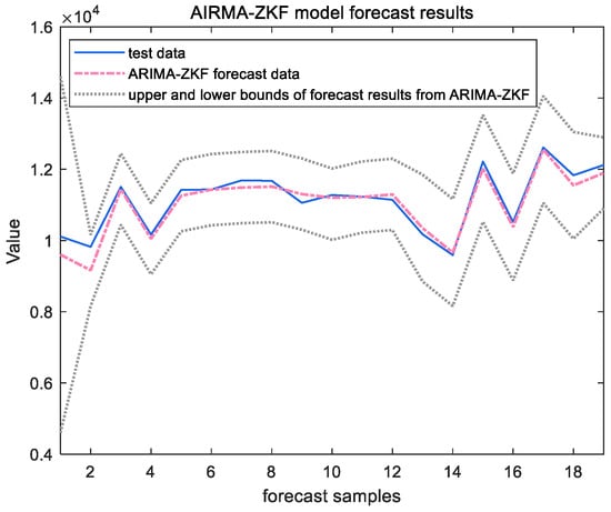
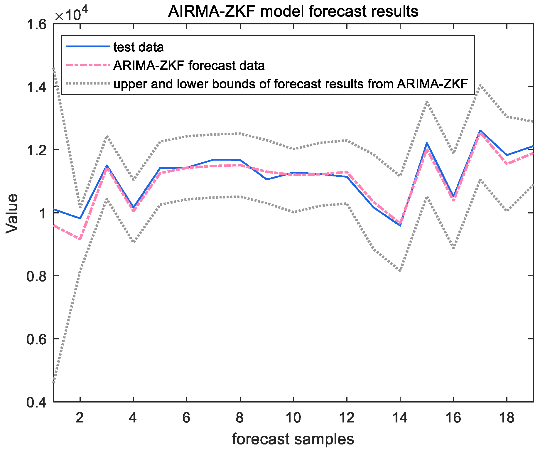
Figure 9.
ARIMA-ZKF model forecast results of Ningbo Zhoushan Port.
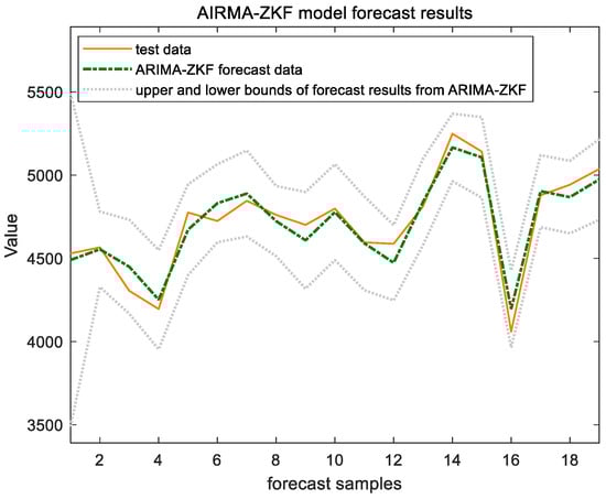
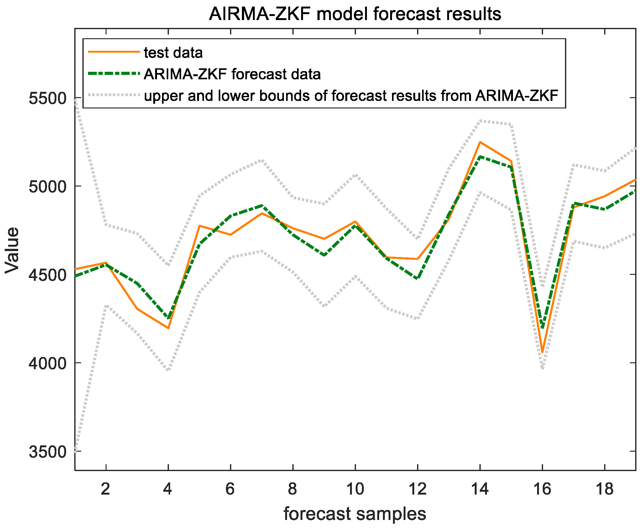
Figure 10.
ARIMA-ZKF model forecast results of Shanghai Port.
The forecast results indicate that the combined model incorporating the ZKF filter performs better in prediction on the test set. This model effectively addresses disturbances within the time series in a timely manner and is capable of synchronizing with and reflecting the data characteristics. These qualities compensate for the ARIMA model’s limitations, such as its inadequate nonlinear mapping ability and the presence of lag. Consequently, the combined model yields a smaller RMSE value and a higher level of prediction accuracy.
3.3. Comparison of Results
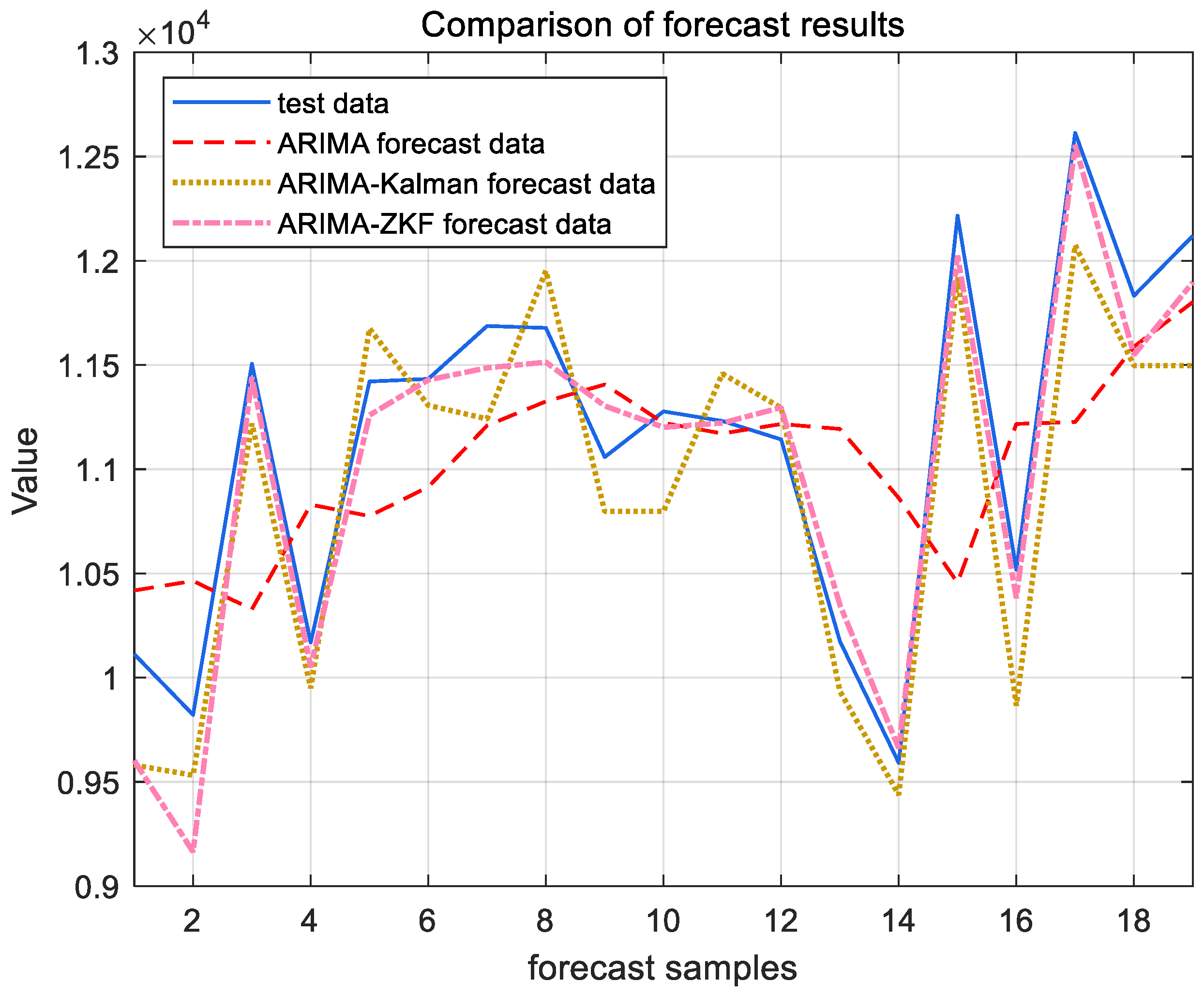
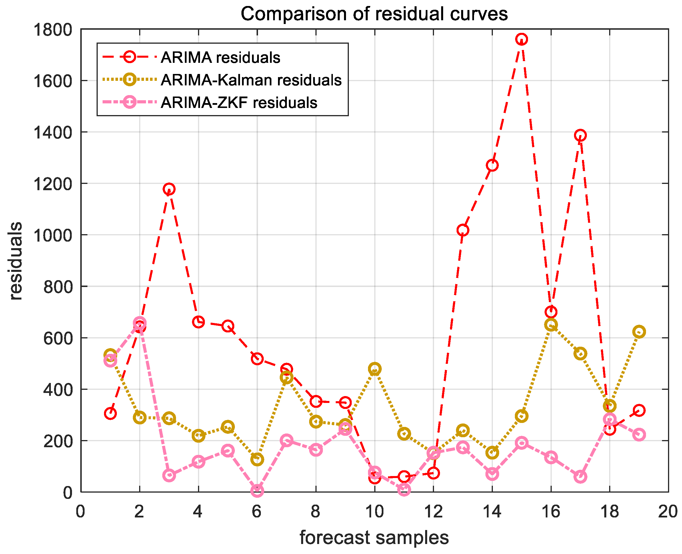
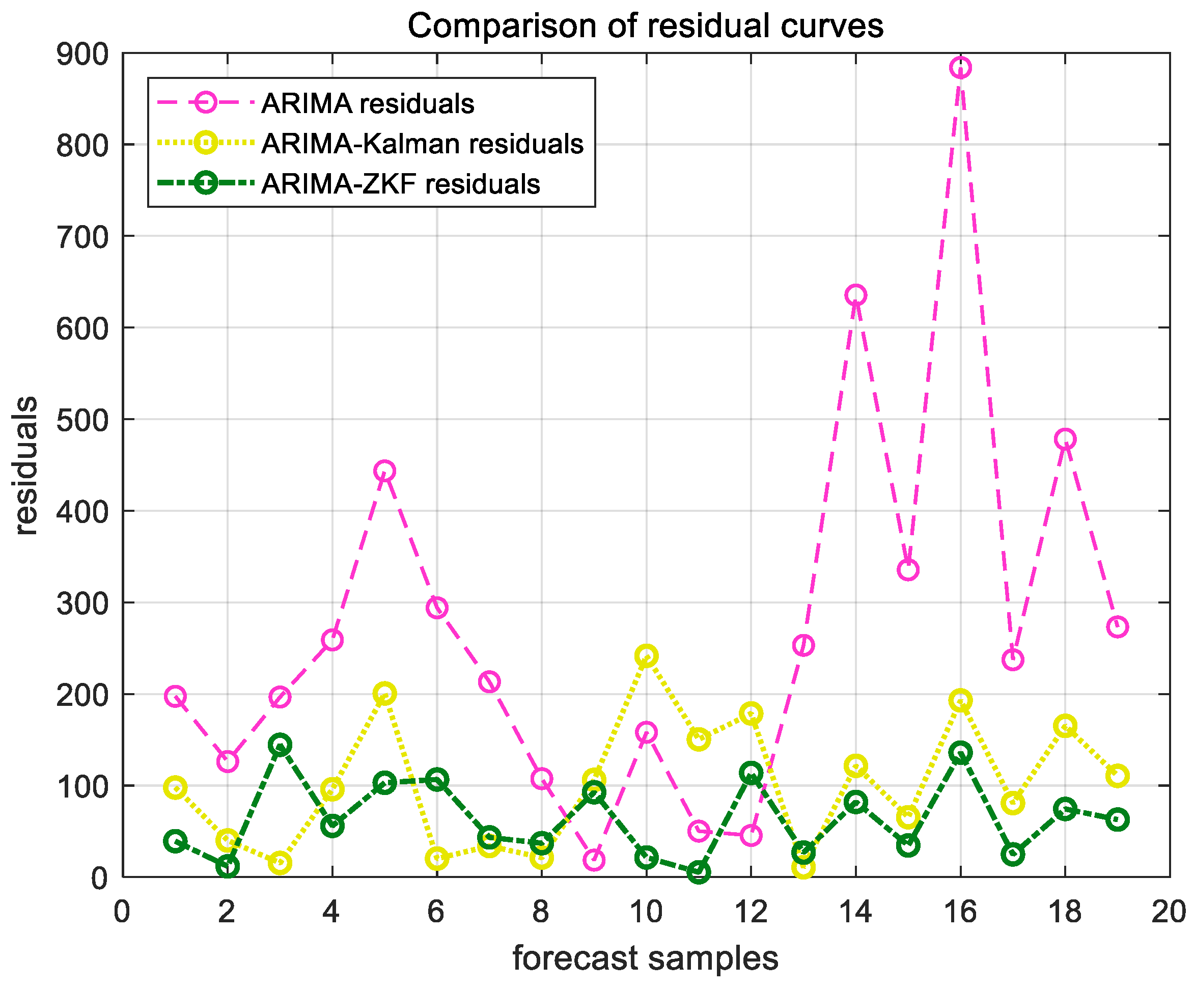
Figure 11 and Figure 12 present the forecast results for the cargo throughput of Ningbo Zhoushan Port and Shanghai Port from November 2022 to May 2024, obtained using the ARIMA model alone and the combined models of ARIMA–Kalman and ARIMA-ZKF. Figure 13 and Figure 14 illustrate the comparative effects of the forecast residual curves of the ARIMA model, ARIMA–Kalman model, and ARIMA-ZKF model, with the vertical axis representing the absolute values of the residuals. Additionally, Table 3 and Table 4 provide the comparative results of the evaluation metrics RMSE and MAPE for the ARIMA model, ARIMA–Kalman model, and ARIMA-ZKF model.
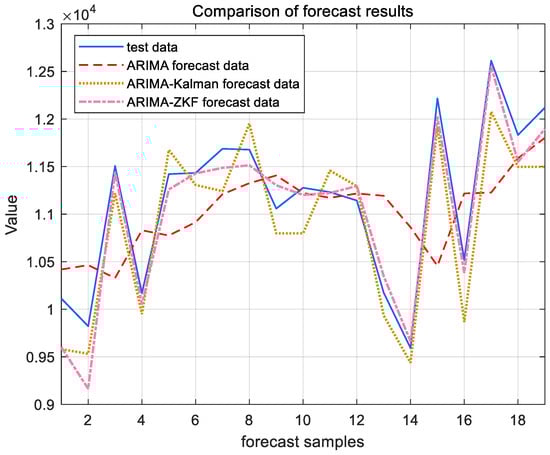
Figure 11.
ARIMA, ARIMA–Kalman, and ARIMA-ZKF models’ forecast results for Ningbo Zhoushan Port.
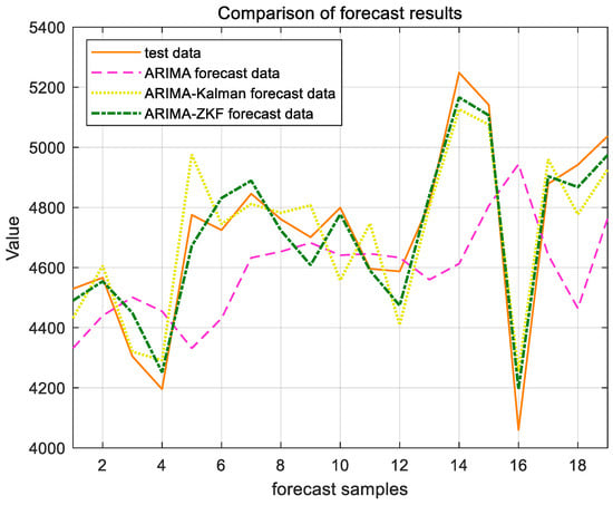
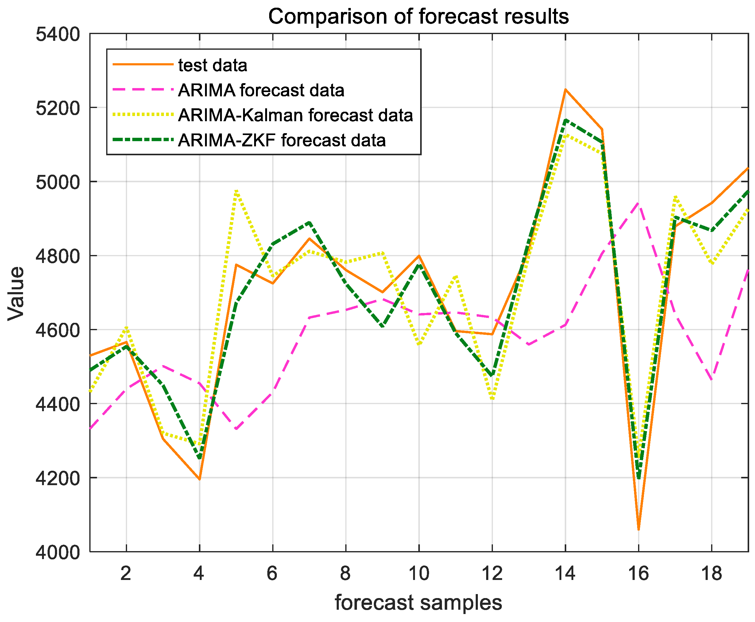
Figure 12.
ARIMA, ARIMA–Kalman, and ARIMA-ZKF models’ forecast results for Shanghai Port.
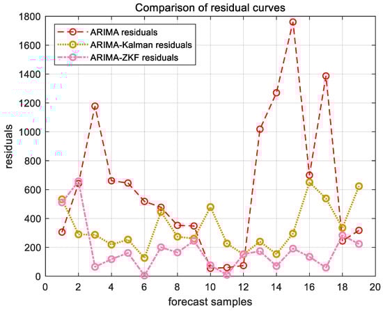
Figure 13.
ARIMA, ARIMA–Kalman, and ARIMA-ZKF models’ forecast residual plots for Ningbo Zhoushan Port.
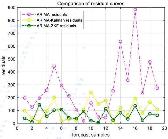
Figure 14.
ARIMA, ARIMA–Kalman, and ARIMA-ZKF models’ forecast residual plots for Shanghai Port.
Table 3.
Comparison of results of model evaluation indicators of Ningbo Zhoushan Port.
Table 4.
Comparison of results of model evaluation indicators of Shanghai Port.
The results demonstrate that the RMSE of the combined ARIMA-ZKF model was reduced by 69.26% and 77.87% in comparison to the ARIMA model, while the MAPE decreased by 4% and 4.48%. Additionally, the prediction accuracy improved from 94.294% to 98.2946% and from 94.13% to 98.62%. The ARIMA-ZKF combined model effectively addressed the issues of an insufficient prediction accuracy and the presence of lag in the ARIMA model. When compared to the ARIMA–Kalman model, the RMSE was reduced by 34.51% and 38.3%, while the prediction accuracy increased by 1.3% and 0.81%. These findings indicate that the ARIMA-ZKF model offers more accurate predictions than both the ARIMA model and the ARIMA model that incorporates the Kalman filter, making it a suitable choice for forecasting port throughput.
4. Conclusions
In this paper, we proposed a combined ARIMA–ZKF prediction model designed for non-stationary time series data characterized by autocorrelation and unknown noise interference. The traditional ARIMA model exhibits hysteresis and asynchrony, which makes it difficult to respond to the rapid changes in data, while the zonotopic Kalman filter can make up for this defect. The parameters of the ARIMA model were first determined to establish the state–space equations, and then the optimal gain matrix and state estimates were obtained by minimizing the generating matrix, and finally, the upper and lower bounds of the time series prediction results wrapped by the hypercube space were obtained, which were constantly corrected in the iteration to obtain more accurate prediction results.
The combined model integrates the statistical characteristics of ARIMA and the real-time processing capability of ZKF, demonstrating an exceptional performance in addressing nonlinear systems, noise interference, and the fluctuations caused by outliers. In the context of port throughput prediction, this combined algorithm combines linear and nonlinear advantages, effectively solves the nonlinear, non-stationary, and multi-source data fusion problems, and has good adaptability and interpretability, which provides a strong basis for port construction planning and decision-making and is not only suitable for Ningbo Zhoushan Port and Shanghai Port but also has an application value for other ports.
From the perspective of sustainable development, the application of this combined ARIMA-ZKF model in port throughput prediction can significantly enhance the long-term sustainability of the port industry. By providing more accurate throughput forecasts, ports can engage in more sustainable supply chain management. This includes better coordination with shipping lines to optimize vessel schedules, thereby reducing waiting times and unnecessary idling, which in turn decreases fuel consumption and greenhouse gas emissions. Moreover, accurate predictions enable ports to plan more effectively for the development of green infrastructure. For example, they can allocate resources more effectively for the construction of energy-efficient berths, the installation of pollution-control equipment, and the implementation of eco-friendly operational procedures. In addition, the enhanced decision-making support provided by the model can help ports proactively adapt to future environmental regulations, ensuring their continued operation in an environmentally responsible manner. This approach not only promotes the sustainable development of individual ports but also has positive spillover effects on the entire maritime transportation ecosystem, fostering a more sustainable and resilient global trade environment.
However, this study also has notable limitations, as it does not account for the actual economic, policy, demographic, and other influencing factors. Future research could explore the integration of neural networks and other modeling approaches to assess the applicability of various models. Additionally, expanding the prediction methodology could enhance its performance and broaden its application in complex real-world scenarios.
Author Contributions
Conceptualization, X.Z.; methodology, X.Z.; software, X.Z.; validation, W.C.; formal analysis, X.Z.; investigation, X.Z.; resources, X.Z.; data curation, X.Z.; writing—original draft preparation, X.Z.; writing—review and editing, X.Z. and W.C.; visualization, X.Z.; supervision, W.C. All authors have read and agreed to the published version of the manuscript.
Funding
This research received no external funding.
Institutional Review Board Statement
Not applicable.
Informed Consent Statement
Not applicable.
Data Availability Statement
Publicly available data from national statistical offices.
Conflicts of Interest
The authors declare no conflicts of interest.
References
- Li, A.; Li, Y.; Xu, Y.Y.; Li, X.M.; Zhang, C.M. Multi-scale convolution enhanced transformer for multivariate long-term time series forecasting. Neural Netw. 2024, 180, 106745. [Google Scholar] [PubMed]
- Xia, L.; Ren, Y.Y.; Wang, Y.H.; Fu, Y.Y.; Zhou, K. A novel dynamic structural adaptive multivariable grey model and its application in China’s solar energy generation forecasting. Energy 2024, 312, 133534. [Google Scholar] [CrossRef]
- Smyl, S.; Bergmeir, C.; Dokumentov, A.; Long, X.Y.; Wibowo, E.; Schmidt, D. Local and global trend Bayesian exponential smoothing models. Int. J. Forecast. 2024, 41, 111–127. [Google Scholar]
- Katić, D.; Krstić, H.; Otković, I.I.; Juričić, H.B. Comparing multiple linear regression and neural network models for predicting heating energy consumption in school buildings in the Federation of Bosnia and Herzegovina. J. Build. Eng. 2024, 97, 110728. [Google Scholar] [CrossRef]
- Fuad, S.; Razaz, S. A unique Markov chain Monte Carlo method for forecasting wind power utilizing time series model. Alex. Eng. J. 2023, 74, 51–63. [Google Scholar]
- Rumbe, G.; Hamasha, M.; Mashaqbeh, S.A. A comparison of Holts-Winter and Artificial Neural Network approach in forecasting: A case study for tent manufacturing industry. Results Eng. 2024, 21, 101899. [Google Scholar] [CrossRef]
- Kim, H.; Park, M. Discovering fashion industry trends in the online news by applying text mining and time series regression analysis. Heliyon 2023, 9, 18048. [Google Scholar]
- Fu, X.Y.; Feng, Z.K.; Cao, H.; Feng, B.F.; Tan, Z.Y.; Xu, Y.S.; Niu, W.J. Enhanced machine learning model via twin support vector regression for streamflow time series forecasting of hydropower reservoir. Energy Rep. 2023, 10, 2623–2639. [Google Scholar]
- Gaertner, B. Geospatial patterns in runoff projections using random forest based forecasting of time-series data for the mid-Atlantic region of the United States. Sci. Total Environ. 2024, 912, 169211. [Google Scholar]
- Bhambu, A.; Gao, R.; Suganthan, P.N. Recurrent ensemble random vector functional link neural network for financial time series forecasting. Appl. Soft Comput. 2024, 161, 111759. [Google Scholar]
- He, C.; Wang, H.P. Container Throughput Forecasting of Tianjin-Hebei Port Group Based on Grey Combination Model. J. Mech. 2021, 2021, 8877865. [Google Scholar] [CrossRef]
- Liang, X.; Wang, Y.; Yang, M. Systemic Modeling and Prediction of Port Container Throughput Using Hybrid Link Analysis in Complex Networks. Systems 2024, 12, 23. [Google Scholar] [CrossRef]
- Wu, W.Y.; Ma, L.; Gao, S.Z. Port container throughput prediction method based on SSA-SVM. Highlights Bus. Econ. Manag. 2023, 12, 88–95. [Google Scholar] [CrossRef]
- Xu, Y.S. Forecast and Analysis of Cargo Throughput and Total Import and Export Volume in Shanghai Port Based on ARIMA Model. Adv. Appl. Math. 2022, 11, 3635–3645. [Google Scholar] [CrossRef]
- Morales-Ramírez, D.; Gracia, M.D.; Mar-Ortiz, J. Forecasting national port cargo throughput movement using autoregressive models. Case Stud. Transp. Policy 2025, 19, 101322. [Google Scholar] [CrossRef]
- Mokhtar, K.; Mhd Ruslan, S.M.; Abu Bakar, A.; Jeevan, J.; Othman, M.R. The Analysis of Container Terminal Throughput Using ARIMA and SARIMA. Springer 2022, 167, 229–243. [Google Scholar]
- Gu, J.; Sui, G.; Li, Z.; Liu, W.; Wang, Y.; Zhan, Y.; Cui, W. Oil well production forecasting method based on ARIMA-Kalman filter data mining model. Shenzhen Daxue Xuebao (Ligong Ban) J. Shenzhen Univ. Sci. Eng. 2018, 35, 575–581. [Google Scholar] [CrossRef]
- Li, P.F.; Wang, Q.Q.; Cao, Q. Prediction Model Based on ARIMA-Kalman Filtering Hybrid Algorithm. Stat. Decis. 2020, 36, 35–38, (In Chinese with English abstract). [Google Scholar]
- Lin, Y.Z.; Wu, X.F.; Lin, M.; Lu, C.; Wan, H.; Chen, Y.Q. A hybrid model of Kalman-ARIMA-LSTM for flow prediction of mine air compressors. In Proceedings of the 2022 19th International Computer Conference on Wavelet Active Media Technology and Information Processing (ICCWAMTIP), Chengdu, China, 16–18 December 2022; pp. 1–7. [Google Scholar]
- Li, Y.T.; Wu, K.; Liu, J. Self-paced ARIMA for robust time series prediction. Knowl. Based Syst. 2023, 269, 110489. [Google Scholar] [CrossRef]
- Zhang, H.P.; Wang, J.Z.; Qian, Y.S.; Li, Q.W. Point and interval wind speed forecasting of multivariate time series based on dual-layer LSTM. Energy 2024, 294, 130875. [Google Scholar] [CrossRef]
- Lyu, J.; Cao, Z.J.; Song, E.B. A data association algorithm for the robust confidence ellipsoid filter. Signal Process. 2023, 213, 109201. [Google Scholar] [CrossRef]
- Khodabandelou, G.; Nakib, A. H-polytope decomposition-based algorithm for continuous optimization. Inf. Sci. 2021, 558, 50–75. [Google Scholar] [CrossRef]
- Ma, X.; Liu, X.G. A data-driven guaranteed zonotopic estimation for unknown time-varying system. ISA Trans. 2024, 155, 164–170. [Google Scholar] [CrossRef]
- Wang, J.; Shi, Y.R.; Zhou, M. Active Fault Detection Based on State Set-membership Estimation. Acta Autom. Sin. 2021, 47, 1087–1097, (In Chinese with English abstract). [Google Scholar]
- Al-Mohamad, A.; Puig, V.; Hoblos, G. Recursive zonotopic set-membership approach for system-level prognostics with application to linear parameter-varying systems. ISA Trans. 2023, 135, 244–260. [Google Scholar]


Disclaimer/Publisher’s Note: The statements, opinions and data contained in all publications are solely those of the individual author(s) and contributor(s) and not of MDPI and/or the editor(s). MDPI and/or the editor(s) disclaim responsibility for any injury to people or property resulting from any ideas, methods, instructions or products referred to in the content. |
© 2025 by the authors. Licensee MDPI, Basel, Switzerland. This article is an open access article distributed under the terms and conditions of the Creative Commons Attribution (CC BY) license (https://creativecommons.org/licenses/by/4.0/).