Transport Carbon Emission Measurement Models and Spatial Patterns Under the Perspective of Land–Sea Integration–Take Tianjin as an Example

Abstract

The goal of “double carbon” puts forward higher requirements for the control of transport carbon emissions, and the exploration of transport carbon emission modelling driven by big data is an important attempt to reduce carbon accurately. Based on the land Vehicle Miles Traveled data (VMT) and the sea Automatic Identification System (AIS) data, this study establishes a refined, high-resolution carbon emission measurement model that incorporates the use of motor vehicles and ships from a bottom-up approach and analyzes the spatial distribution characteristics of land and sea transport carbon emissions in Tianjin using geospatial analysis. The results of the study show that (1) the transportation carbon emissions in Tianjin mainly come from land road traffic, with small passenger cars contributing the most to the emissions; (2) high carbon emission zones are concentrated in economically developed, densely populated, and high road network density areas, such as the urban center Binhai New Area, and the marine functional zone of Tianjin; (3) carbon emission values are generally higher in the segments where ports, airports, and interchanges are connected. The transportation carbon emission measurement model developed in this study provides practical, replicable, and scalable insights for other coastal cities.

1. Introduction

Global warming has become a major challenge facing human development, and the international community is currently paying close attention to the environmental issues caused by the excessive emissions of greenhouse gases such as carbon dioxide. In 2020, China proposed the “dual carbon” goal, which aims to reasonably control carbon dioxide emissions to peak before 2030 and strive to achieve carbon neutrality by 2060 [1]. Currently, China is in a critical period of the 14th Five-Year Plan, which also represents a key window for achieving the “dual carbon” goals. Therefore, how to effectively control carbon dioxide emissions while promoting economic development has become an urgent issue to be addressed [2,3].

According to a report by the International Energy Agency (IEA), the transportation sector has become one of the fastest-growing areas for greenhouse gas emissions in recent years [4]. In terms of land transportation, the dense operation of motor vehicles in urban road systems is a major source of carbon emissions, particularly in urban centers and transportation hubs, where carbon emissions tend to remain high. In the maritime transportation sector, ship operations and logistics activities at ports generate substantial carbon emissions. This not only affects the environmental quality of the port itself but also influences the city’s overall carbon footprint through land–sea intermodal transportation [5]. In recent years, decarbonization measures for ports (such as shore power technology, the promotion of clean fuels, and intelligent scheduling) have been gradually promoted internationally [6]. However, coordination and integration between these measures and land transportation management still lack. Based on geographic traffic mobile source data, analyzing the carbon emission characteristics and spatial distribution of different transportation modes under various influencing factors is of great significance for achieving precise emission reduction in the transportation sector [7].

China has a long coastline with numerous coastal cities, favorable geographic locations, and convenient transportation. Coastal cities have become the most dynamic emerging economic zones in the country’s economic development [8,9]. However, coastal cities face dual pressures of transportation carbon emissions from both land and sea, with a conflict between economic development and transportation energy consumption. The 2023 “National Carbon Peak Pilot Construction Plan” clearly outlines the selection of 100 representative cities and districts across the country for carbon peak pilot projects, including several coastal cities such as Qingdao and Yantai [10,11]. Against this backdrop, developing a scientific model for calculating transportation carbon emissions in coastal cities and systematically planning and exploring green emission reduction and decarbonization in the transportation sector has become a practical necessity for coastal cities to implement precise emissions reduction and source-based governance under the “dual carbon” goals [12,13].

To achieve the “dual carbon” goals and control transportation carbon emissions, it is essential to conduct in-depth research on their mechanisms and spatial distribution. Scholars, both domestically and internationally, have conducted extensive studies on methods for calculating carbon dioxide emissions from transportation, providing a basis for policy formulation and decision-making support [14,15,16]. At present, the “top-down” measurement method and the “bottom-up” carbon emission measurement method proposed by the IPCC (Intergovernmental Panel on Climate Change) are generally accepted internationally [17]. The “top-down” approach is to measure the total transport carbon emissions based on the transport energy consumption and the corresponding energy–carbon emission factors. For example, Han et al. measured the carbon emissions from China’s transport sector from 1995 to 2014 using yearbook data based on the “top-down” method and further analyzed the relationship between transport carbon emissions and GDP [18]. Liu et al., using the STIRPAT and GTWR models and data from the transportation sectors of 30 provinces from 2003 to 2017, estimated the carbon emission intensity of China’s transportation industry and revealed, from a spatiotemporal perspective, the impact of its driving factors on carbon emission intensity [19]. Dong Mengru et al., using maritime statistical data and employing a “top-down” approach, estimated the carbon emissions from China’s maritime transport and analyzed its carbon emission efficiency [20]. In general, the “top-down” estimation method is effective primarily for macro-level assessments of transportation carbon emissions.

The “bottom-up” method is based on mileage, motor vehicle ownership, energy consumption per mile, energy consumption structure of different modes of transport and the corresponding localized emission factors to measure transport carbon emissions. For example, Palencia et al. estimated the penetration rate of the Japanese automobile market through an optimization model and used the inventory turnover data to measure the transport carbon emissions of the Japanese automobile industry based on the “bottom-up” method [21]. Lejda et al. used petrol and natural gas passenger car data to measure the transport carbon emissions of old and new vehicles, in and out of the laboratory, in a region of Poland, based on a “bottom-up” approach [22]; Hao et al. used freight turnover data and ship voyage data to measure the transport carbon emissions of inland waterway, coastal, and ocean freight transport in a region of China, for the period of 2006–2012, based on a “bottom-up” approach [23]; Villalba and Styhre, using ship carbon emission data and employing a “bottom-up” approach, estimated the transportation carbon emissions of major global ports, including the Mediterranean gateway ports of Barcelona, as well as the ports of Gothenburg, Long Beach, Osaka, and Sydney, across four continents [24,25]. Weng Shujuan et al. used various types of passenger and cargo ships in Guangdong Province as the research object and, based on the “bottom-up” method, the CO₂ emission inventory of ships from 2006 to 2020 was calculated, and the carbon emission paths and potentials of ships in Guangdong Province were predicted [26]. In general, the “bottom-up” approach is mainly based on the mileage and energy consumption of different modes of transport to project the total energy consumption. Compared to the “top-down” approach, the “bottom-up” method allows for more precise calculation of micro-level carbon emissions and can distinguish carbon emissions from different modes of transport, facilitating comparative studies of the horizontal carbon emission differences between transport modes [27].

In the above analysis, scholars at home and abroad have carried out many measurements and analyses of transport carbon emissions, but there is a lack of studies that consider and measure transport carbon emissions from land and sea in a comprehensive manner for the characteristics of coastal cities, which makes it difficult to provide practical scientific decision support for precise emission reduction and coordinated carbon reduction in coastal cities. In view of this, this study proposes to adopt the IPCC “bottom-up” measurement method and take Tianjin, an important coastal city in China, as an example. Based on the AIS (Automatic Identification System) and Vehicle Miles Traveled (VMT) data, we constructed a full-sample, fine-grained carbon emission measurement model that includes carbon emissions from both land and sea transport, and investigated the carbon emissions generated by various modes of transport and their spatial distribution characteristics in Tianjin.

This study intends to solve the following scientific problems: (1) Integrating land space and sea space, constructing a comprehensive assessment framework of carbon emissions from transport in coastal cities in land space and sea space, and attempting to fit a multi-sample, high-precision carbon emissions measurement model, that includes land and sea transport, in order to achieve a comprehensive analysis of the characteristics of the spatial distribution of carbon emissions in coastal cities or regions. (2) Based on the VTM data and AIS data of transport big data, we will visualize the spatial layout of the grid under the regional distribution of high-value road sections, waterways and administrative units of land, and sea transport carbon emissions, so as to promote the service of the “dual-carbon” target in the field of transport at the practical level. (3) Based on the carbon emission classification data of land and sea transport vehicles, clarify the types of high-value sources of carbon emission of various land and sea transport vehicles, and reveal the characteristics of transport carbon emission in the land space of typical coastal cities.

2. Study Area and Data Processing

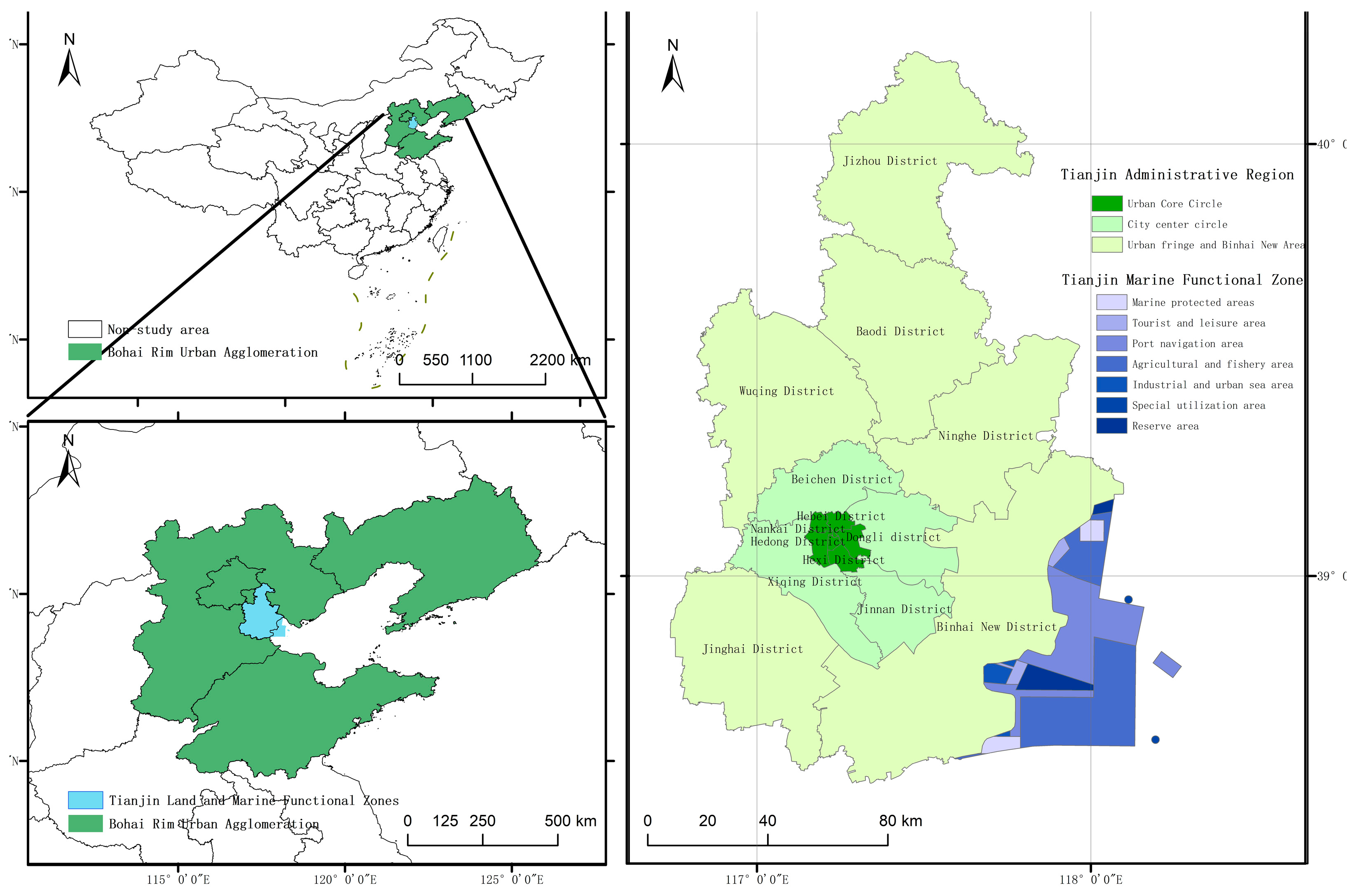
2.1. Overview of the Study Area

The study area of this paper includes the whole part of Tianjin’s land administrative area and its functional marine area, the specific location is shown in Figure 1. Tianjin is bordered by the Bohai Sea to the east, Yanshan Mountain to the north, Beijing, the capital city, to the west, and Hebei Province to the rest. It is the transportation throat of the railroad to Northeast China and East China and an important port for ocean shipping, the main node of the China–Mongolia–Russia Economic Corridor, the strategic pivot of the Maritime Silk Road, and the intersection of “One Belt, One Road”. The internal hinterland is vast, with radiation in North China, Northeast China, Northwest China, 13 provinces and autonomous regions, and externally facing Northeast Asia. Tianjin is the largest port city in northern China, and is an important northern international shipping core [28]. In 2023, Tianjin’s GDP was 167.373 billion yuan, and the annual freight volume was 539.636 million tonnes, of which the cumulative cargo transportation volume of road was 303.82 million tonnes and water transportation 107.6 million tonnes, accounting for 76.2% of the total freight volume. By the end of 2023, the number of civilian cars in Tianjin was 4,186,600, of which 3,682,500 were private cars; the Maritime Safety Administration registered 1314 ships with a total tonnage of 6.72 million tonnes (Tianjin Statistical Yearbook 2024).

Tianjin’s traffic operation mileage and traffic development level are among the highest in the country. The highway network forms a network system with national highways and some municipal trunk routes as the backbone and radial highways as the main system, with the outer ring road communicating the connection of each radial highway. There are four main national highways passing through Tianjin: Beijing-Tianjin-Tanggu Expressway, Beijing-Fu Class I Automobile Highway, Ladan Expressway, and Jin-Tang Branch of Ladan Expressway. In 2022, Tianjin’s transport end-use energy consumption will be 5,901,500 tonnes of coal, which will account for 7.2% of the industry’s total energy consumption, far exceeding the transport industry’s economic share of 5.8% (China Energy Statistical Yearbook 2022). Therefore, taking Tianjin as a typical study area of coastal cities, establishing an accurate measurement model of transport carbon emissions is of great significance for other coastal cities to provide operable, replicable, and scalable experiences.

2.2. Data Sources and Pre-Processing

In this paper, due to the limitation of data and other objective conditions, the measurement of carbon emissions from transport only includes carbon emissions from road transport in the land area and carbon emissions from shipping in the seaports and excludes carbon emissions from air transport and carbon emissions from railway transport. The data sources in this paper mainly include two categories: (1) land transport data and (2) marine AIS ship data. The land transport data include open street data, car ownership, average daily road traffic, and labelled fuel economy (LFE) data. The open street data used in this paper comes from the National Centre for Basic Geographic Information; the regional car ownership data comes from the Tianjin Statistical Yearbook; the VMT data and the regional average daily traffic volume on the roads are obtained from the Tianjin Unified Open Platform for Information Resources VMT, and average daily traffic volume of regional roads are calculated by analyzing and processing the measured road traffic data obtained through the AIP interface provided by Tianjin Information Resources Unified Open Platform, which is integrated with the model below. The specific research framework is shown in Figure 2.

The VMT data was predicted using corrected 24-h road traffic volume (AADT) data by referring to the Highway Monitoring System (HPMS) method published by the U.S. Environmental Protection Agency (EPA) and the U.S. Federal Highway Administration (FHWA). AADA is then combined with road vector data and expansion factors to obtain road traffic VMT for the entire region. As an important indicator of urban vitality and traffic energy consumption, road intersections have been shown to have a significant correlation with traffic energy consumption [29]. In this paper, we use ArcGIS to obtain the VMT of road traffic in the whole region. In this paper, we extracted and counted the number of road intersections with the help of Network Analyst Tools and Spatial Analyst Tools in ArcGIS, and used the data of road length, road grade, and the number of road intersections to present the value of road traffic carbon emissions in Tianjin on different grades of highways in various districts and counties, and analyzed the carbon emission data accordingly.

The marine AIS ship database consists of AIS ship dynamic information data and ship static files. The ship dynamic AIS data of Tianjin port used in this paper comes from the land, sea, and air satellite integration network of ShipHub, and the spatial scope is selected to be 117.30°~118.15° E, 38.36°~39.35° N of the marine functional zoning range of Tianjin, and a total of 32 GB of ship sailing trajectory point of 2019 within the study area is extracted data, with an average reporting interval of 3 min. The ship static base data were obtained from the China Classification Society and Lloyd’s database. The dynamic vessel position data records of fishing vessels include attributes such as vessel name, MMSI code (vessel water mobile communication service identification code), longitude, latitude, speed, heading, time, etc., and the basic static data records of fishing vessels include attributes such as vessel name, MMSI code, main engine power, operation type, and maximum speed.

AIS message information between the ships is based on the coding mechanism for transmission, so it is necessary to decode and translate the AIS message information in order to obtain the data that can be read and participate in the calculation. The decoded AIS data has a certain degree of discrete information and, in the process of transmission, the data may be subject to poor communication signals, equipment damage and ageing, and other objective factors, so it is necessary to process the data to make it readable and eliminate its abnormal values so that it can be reasonably used.

In this paper, the preprocessing of AIS data mainly uses the following three steps: ① cleaning the AIS data of obvious anomalies, errors, and repetitive data; ② eliminating the AIS data that is out of the range of the area, deviating from the trajectory, and without true speed, and adopting the propagation of the speed limit threshold to eliminate the unreasonable data of the supercritical, so as to smooth the ship’s overall speed (as shown in the specific model expression in Equation (1)); ③ using the MMSI coding to match and reconstruct the dynamic and static datasets of the fishing vessels on a traversal-by-traversal basis. A vessel database can be formed for direct use in the calculation, according to which the corresponding statistical analyses of the carbon emission data can be carried out.

$$\left|\beta \right|=\left|(v_a-v_c)/v_c\right|>50\%$$

(1)

where |β| is the relative speed deviation ratio, defined as the absolute difference between the average speed ($v_a$) and the current AIS-reported speed ($v_c$), normalized by $v_c$. This ratio is dimensionless and serves as a threshold for identifying anomalous speed data.

3. Transport Carbon Emission Measurement Model

3.1. Carbon Emission Measurement Models for Land-Based Road Transport

Unlike common point source and surface source data, motor vehicles, as a typical mobile carbon emission source in road transport, have a certain complexity in their measurement [30]. Taking urban road traffic as an example, the carbon emission accounting model for land transport is shown in Equation (2):

$$E_{road}={\sum }_{i=1}^n[V{P}_i\times VM{T}_i\times RF{E}_{ig/d}\times CE{F}_{ig/d}]\times {10}^{-6}$$

(2)

where $E_{road}$ is the CO₂ emissions from land-based road traffic in tonnes; VP is the number of motor vehicles in units; VMT is the average annual mileage travelled in units of kilometers per vehicle (km/vehicle); RFE (on-Road Fuel Economy) is the fuel economy of the vehicle in units of kilometers per litre (L/km); CEF (Carbon Emission Factor) in tonnes per litre (g/L); $i$ is the different motor vehicle types; $g$ is petrol; and $d$ is diesel.

In calculating carbon emissions from land-based road transport, this study refers to the model document “Types of Motor Vehicles for Road Traffic Management”, which classifies motor vehicles into three types: passenger cars, goods vehicles, and other types of motor vehicles. Among them, passenger cars are subdivided into large, medium, small, and micro, goods vehicles are subdivided into heavy, medium, light, and micro, and other types of motor vehicles are mainly motorbikes. Based on these classifications, this study obtains data on carbon emissions from nine different types of motor vehicles and summarizes these data.

3.1.1. Fuel Economy (RFE) Determination

In early studies, the calculation of fuel economy was primarily based on test data under standardized conditions, which typically assumed an ideal driving environment. However, real-world driving is influenced by multiple factors, leading to significant deviations from standardized conditions [31]. Therefore, in order to more accurately assess a vehicle’s fuel economy during actual use, researchers have gradually developed correction models to adjust laboratory test values, making them more representative of real-world fuel consumption [32]. The modification model for the actual RFE value of the vehicle is represented by Equation (3).

$$RF{E}_i={\alpha }_i\times LF{E}_i$$

(3)

where RFE denotes the actual road fuel consumption of model class $i$ in litres per 100 km (L/100 km); ${\alpha }_i$ denotes the combined correction factor for model class $i$; $LF{E}_i$ denotes the combined fuel consumption of model class $i$ in litres per 100 km (L/100 km).

LFE represents the ratio of fuel consumption to mileage under optimal driving conditions for each vehicle type and is a measure of vehicle fuel economy, which can be determined based on the level of fuel consumption tested under standard operating conditions, i.e., the combined fuel consumption, provided by the standard vehicle manuals for each type of vehicle. However, the actual use of each vehicle is not a standard working condition situation, so it is necessary to combine the actual use of each motor vehicle’s working conditions, including vehicle design, driving style, age, driving speed, etc., to carry out a certain revision of the localization factors, such as the quality of the fuel, the road conditions and the percentage of cold weather in the local area, etc., and the present study has set a certain correction factor for the working conditions of the vehicles travelling in the study area for improvement based on the references [33,34].

3.1.2. Motor Vehicle Emission Factor (CEF) Determination

The emission factors of different regions and types of motor vehicles are affected by a variety of factors, such as local temperature, road conditions, and the vehicle’s own driving conditions, all of which affect the vehicle’s carbon emission factor [35]. At low temperatures, cold-start engine emissions are significantly higher than at ambient temperatures, resulting in higher emission factors. In terms of driving conditions, when the vehicle speed is low, the engine load is small and the fuel cannot be fully burned, thus increasing the emission factor. In addition, the quality of oil is also one of the factors affecting the emission factor, and the olefin content and sulphur content, etc., will affect the combustion of the engine and the efficiency of exhaust gas treatment [36].

In this study, the carbon emissions of diesel and petrol from motor vehicles are adjusted by taking into account the specific conditions of geography, meteorology, and temperature in Tianjin. The specific model expression is shown in calculation Formula (4):

$$CE{F}_{i,j}=BE{F}_i\times {\phi }_{ij}\times {\gamma }_i\times {\lambda }_i\times {\theta }_i$$

(4)

where CFF is the emission factor of class $i$ vehicle in region $j$, BEF (Baseline emission factors) denotes the comprehensive baseline emission factor of class $i$ vehicle, ${\phi }_{ij}$ denotes the meteorological correction factor of class $i$ vehicle in region $j$, ${\gamma }_i$ denotes the correction factor of the average speed of the vehicle travelling in region $j$, ${\lambda }_i$ denotes the deterioration correction factor of class $i$ vehicle, and $\theta$ denotes the correction factor of other usage conditions (e.g., load factor, oil quality, etc.) of class $i$ vehicle. The calculation method and selection of emission factors in this study are based on the technical guidelines for the compilation of the road motor vehicle air pollutant emission inventory published by the Ministry of Environmental Protection of China.

3.2. Carbon Emission Measurement Models for Marine Traffic

Based on the ship activity data provided by AIS and the ship attribute information data provided by Lloyd’s database and CCS ship catalogue, this study constructs a carbon emission measurement model for ships and uses the power method to measure the emission inventory of ships in the sea area near Tianjin. The basic parameters of the model include the rated power of the main and auxiliary engines of the ship, the load power of the main and auxiliary engines of the ship, the load factor of the main and auxiliary engines of the ship, and the carbon emission factors of various types of ships under different operating conditions, and the calculation expression of the model is shown in Equation (5):

$$E_{ship}={\displaystyle \sum _{i=1}^s{\displaystyle \sum _{i=1}^c(R{P}_{si}\times L{F}_{sci}\times T_{sci}\times CE{F}_{sci}\times {10}^{-6})}}$$

(5)

In the formula, E_Ship is the emission from the ship in tonnes (t); RP (Rated Power) is the rated power of the ship’s engine in kilowatts (kw); LF (Load Factor) is the load factor of the engine; T (Time) is the ship’s sailing time in hours (h); CEF is the carbon emission factor of the ship, and the unit is grams per kilowatt hour (g/KWh); $i$ is different types of ships; s is the emission source of launching, which is mainly divided into the main engine and the auxiliary engine; c is the navigational state of the ship, which is mainly divided into the following four operating conditions: cruising condition, motorized manoeuvring condition, hoteling condition, and anchoring condition, and the emission of the ship under each condition is divided into different categories according to the main engine (main engine) and auxiliary engine (auxiliary engine) in different working conditions.

3.2.1. Determination of Ship Engine Power (RP)

The engine power of a ship is mainly obtained by relying on the ship database of the MMSI number in the AIS information compared with the static information of the ship. For some of the unobtained ship engine power, the rated power of the ship’s main engine and the rated power of the secondary engine are fitted to calculate the rated power of the ship’s main engine and the rated power of the auxiliary engine based on the relational equation between the ship’s main engine, the rated power of the auxiliary engine, the design speed, and the ship’s gross tonnage. Specifically, this study uses the relationship equation between the ship’s gross tonnage (GT), the ship’s design speed (V_d), and the ship’s main and auxiliary engines’ rated power, to derive the ship’s main engine’s rated power (RP₁), the auxiliary engine’s rated power (RP₂), and V_d, in which the RP₂ is computed by taking the mean after comparing it with the RP₁.

Because the study area of this paper belongs to the Bohai Sea area, the fitting formula of Xing Hui’s carbon emission measurement for maritime transport in the Bohai Bay area is used to calculate the carbon emissions of cargo ships, passenger ships, and passenger ships [37]. RP₁, RP_2, and V_d for cargo ships, passenger ships, and oil tankers are used to calculate the carbon emissions from marine transport, while fishing vessels and tugboats are fitted with the known RP₁, RP₂, V_d and GT to obtain the functional relationship model, and the specific fitted model is shown in

Table 1. Fits the relationship between the ship’s main and auxiliary engine ratings, design speed and ship’s gross tonnage. Note: R² Values are coefficients of determination, N denotes fitted sample size, $\bar{x}$ is the mean, s is the standard deviation, and *, **, *** denote statistical significance at the 1 per cent, 5 per cent, and 10 per cent levels, respectively. Source: [37].

Ship Type (N)	RP1 (R2 )	RP2/RP1 ($\bar{x}$ ± s)	Vd (R2)
Cargo ships (655)	RP1=3.863 × GT0.785 (0.788) ***	0.28 ± 0.11	Vd = 4.107 × GT0.131 (0.981) ***
Passenger ships (119)	RP1 = 2.067 × GT0.865 (0.863) ***	0.21 ± 0.06	Vd = 3.454 × GT0.170 (0.751) ***
Tankers (352)	RP1 = 8.084 × GT0.681 (0.932) ***	0.26 ± 0.09	Vd = 5.471 × GT0.094 (0.648) ***
Fishing vessels (127)	RP1 = 13.315 × GT0.689 (0.814) ***	0.22 ± 0.07	Vd = 4.344 × GT0.159 (0.745) ***
Tugboat (131)	RP1 = 11.657 × GT0.689 (0.674) ***	0.25 ± 0.08	Vd = 5.047 × GT0.089 (0.689) ***

. The table includes the five main ship types in the study area, including cargo ships, passenger ships, fishing vessels, tankers, and tugs. To ensure the accuracy of the analyses of ship types, the remaining ship types that make up a very small percentage of the study area were excluded from the analyses.

3.2.2. Determination of Ship Engine Load Factor (LF)

Load factor refers to the actual operating power of a ship’s loaded engine and the proportion of the rated power of the ship’s power unit under different speeds. Since ships are often affected by many factors, such as ocean, weather and cargo capacity, during operation, the maximum operating power of a ship will change. In this paper, the rated power of a ship’s engine is multiplied by the corresponding loading coefficient to simulate the ship’s actual navigational state, so as to make the ship’s exhaust emission inventory close to the real situation.

(1)

Load factor of the main engine:

The ship’s main engine is an important power device for ship navigation, mainly relying on the ship’s propeller against the resistance of seawater, and the specific ship host load factor can be calculated according to the basic principles of the propeller (Propeller) [38]. The calculation of the specific model is shown in Equation (6):

$$LF={(V_a\times V_d)}^3$$

(6)

where LF represents the load factor of the ship’s main engine (percent), V_a represents the ship’s actual sailing speed, and V_d represents the ship’s design speed. Under the normal navigation state of the ship, the actual navigation speed will not be greater than the design speed, and when the calculation result LF is greater than 1, it will be set to 1 by default in this study, so as to complete the calculation of the measurement model.

(2)

Load factor for the auxiliary engine:

The load factor of the auxiliary engine cannot be calculated using a formula; it is primarily influenced by two factors: the ship type and the ship’s sailing state. This paper combines several sources of literature to establish the load factor for the auxiliary engine used in ship exhaust emission inventories [39,40,41], and the load factor of the auxiliary engine in this paper is shown in

Table 2. Load coefficients of the auxiliary engine for each ship type under different sailing conditions.

Ship Type	Cargo Ship	Passenger Ship	Tankers	Tugboat	Fishing Vessel
Underway	0.17	0.80	0.13	0.17	0.17
Slow Speed	0.27	0.80	0.27	0.27	0.27
Maneuvering	0.45	0.80	0.45	0.45	0.45
Hoteling	0.22	0.64	0.67	0.22	0.10
Cited Material	[39]	[41]	[39]	[39]	[39]

:

3.2.3. Determination of Emission Factors (CEF) for Ship Engines

The emission factor is an important parameter to establish the calculation of carbon emissions from ships, and the selection of this parameter directly determines whether the results of the measurement of emissions from ships are reasonable and accurate. In the study of the emission inventory of ship emissions, the selection of emission factors mainly comes from two aspects: ① the value of the emission factor is obtained through a large number of tests and experiments; ② the recognized, widely used and more accurate authoritative emission factors are selected as the measurement parameters for the study. Emission factors were first proposed by Eyring et al. and have gradually been recognized and used [42]. There is no uniform international regulation on the selection of emission factors for marine vessels, and the most authoritative CO₂ emission factors are currently provided by the IPCC [17].

Chinese scholars Xing Hui and Duan Shulin et al. analyzed a marine diesel engine based on the emission test report of a mother-type engine and determined the CO₂ emission factors based on work done for the two-stroke main engine and four-stroke sub-engine [43]. In this study, the emission factors of the main engine and the secondary engine of the ships will be set based on the emission factors provided by the Forth IMO GHG Study [41], the emission factors provided by the IPCC [17], the emission factors selected by Wang Chengjie et al. in their study of the exhaust emissions of ocean-going vessels in the Dalian sea area [44], and the emission factors selected by Zeng Fantao et al. in their study of the emission inventory of boats in Xiamen Harbor [45].

(1)

Emission factor for the main engine:

In this study, the main engine of the ship is divided into two kinds of low-speed diesel engines and medium-speed diesel engines, and the specific division principle is based on the data provided by Wang on the types of machines loaded under different tonnages for each ship type [12]. The default type of fuel consumed by the main engine is heavy oil with a sulphur content of 2.7%, and the carbon emission factor of the main engine of the ship is 620 g/KWh under the low-speed diesel engine-1, and the carbon emission factor of the main engine is 683 g/KWh under the medium-speed diesel engine-1 [39].

(2)

Emission factor for the auxiliary engine:

The type of diesel engine of the marine auxiliary engine is not differentiated, the fuel consumed by the auxiliary engine defaults to heavy oil with 2.7 per cent sulphur content, and the auxiliary emission factor defaults to 683 g/KWh.

4. Results

4.1. Spatial Characteristics of Carbon Emissions from Land and Sea Transport in Tianjin

In order to express the results of transport carbon emissions with high-precision geospatial features, this paper adopts a 1 km × 1 km resolution spatial grid to visualize the carbon emissions from sea and land transport in Tianjin, and the obtained results of the Tianjin sea and land carbon emissions traffic map visualization are shown in Figure 3. From the overall view, the total transport carbon emission in Tianjin in 2019 is 7.980 million tonnes, of which the 7.6059 million tonnes of carbon emission from land transport account for 95.3% of the total carbon emission, and the 374,400 tonnes of carbon emission from marine transport accounts for 4.7% of the total carbon emission, and the transport carbon emission mainly comes from land transport.

From the perspective of the types of Tianjin’s transport carbon emissions, Tianjin’s transport carbon emissions mainly come from vehicle carbon emissions, such as small passenger cars, light goods vehicles, heavy goods vehicles, etc. Small passenger cars (i.e., common cars) have the greatest impact, with a carbon emission value of 5.98 million tonnes, accounting for 95.99% of the carbon emissions from vehicles, and accounting for 74.95% of the overall carbon emissions. The values of carbon emissions from land cargo vehicles and carbon emissions from marine vessels in Tianjin are closer, at 1,324,100 tonnes and 374,400 tonnes respectively, accounting for 16.59% and 4.7% of the total value of carbon emissions.

The spatial distribution of carbon emissions in Tianjin is characterized by the following: (1) High-value carbon emission zones are widely distributed in economically developed and densely populated areas, mainly in the urban center of Tianjin, the Binhai New District, and the Tianjin Marine Functional Areas, such as Heping District, Hedong District, Hexi District, Binhai New District, and the port and shipping areas and the industrial and urban sea use areas within the scope of marine functional zones. These areas have relatively developed economies, concentrated populations, and high road network density. (2) Low-value carbon emission zones are concentrated in the peripheral districts and counties of Tianjin, and the agricultural and fishery zones and marine protected areas within the scope of the marine functional zones, such as the Jinghai and Jizhou districts, and the southeastern Tianjin agricultural and fishery zones and the Dagang Coastal Wetland Marine Special Protected Area within the marine functional zones. (3) The major ports and harbours of Tianjin and their routes have high values of carbon emission. The carbon emission values of airports and overpass sections are generally high, and such areas are mainly located in the intersection areas of sea and land transport. The airport logistics center near the Tianjin airport has a high traffic carbon emission value, and the areas with high traffic carbon emission density also include the road sections connected by overpasses, which are the places where traffic flows converge in multiple road sections, and the carbon emission value is relatively high.

4.2. Spatial Characteristics of Carbon Emissions from Different Types of Land and Sea Transport Modes

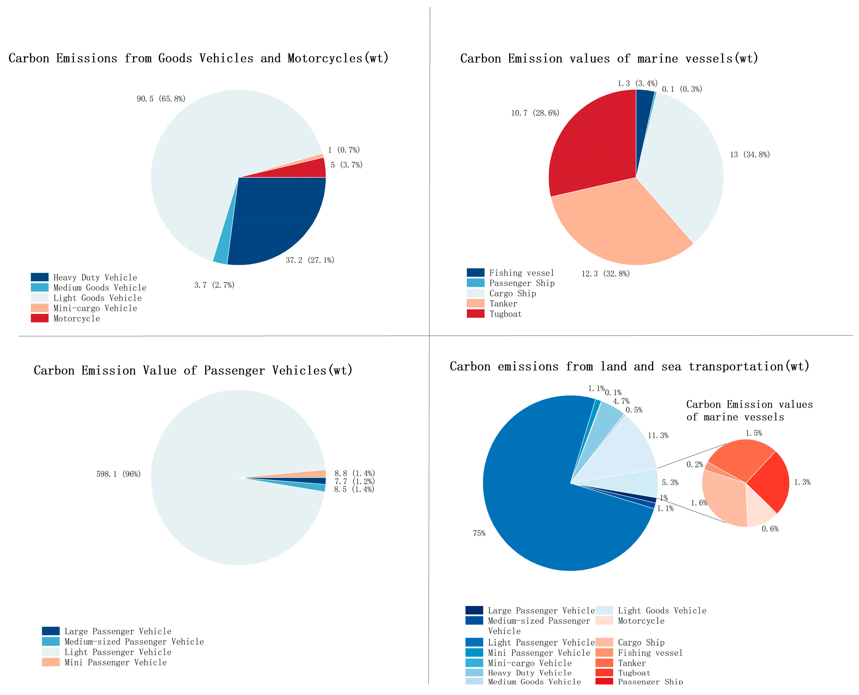
4.2.1. Characteristics of Carbon Emissions from Land-Based Vehicular Transport

Carbon emissions from land transport are divided into three main categories: passenger cars, goods vehicles, and other types. As shown in Figure 4, the carbon emission share of the three types of transport varies considerably, with passenger cars accounting for the highest share of carbon emissions, at 81.93 per cent, mainly because of their extremely large number of motor vehicles, accounting for 89.49 per cent of the total number of vehicles. Goods vehicles and motorbikes accounted for a relatively small share of carbon emissions, 17.4 per cent and 0.67 per cent respectively. Among the categories of passenger vehicles, small buses (i.e., family buses) accounted for a high proportion of carbon emissions due to the high proportion of ownership, which has been increasing year by year, while large buses, medium buses and small buses accounted for a smaller and more balanced proportion. Among the categories of goods vehicles, the proportion of light goods vehicles is the highest, and light goods vehicles emit more carbon, totalling 904,800 tonnes, due to their high ownership, fewer constraints on driving in urban areas and longer mileage compared with heavy and medium goods vehicles. Heavy-duty trucks came next, with a higher ownership and a total carbon emission of 372,000 tonnes due to Tianjin’s role as a land and sea transport hub and the rapid economic growth of the logistics industry.

4.2.2. Characteristics of Carbon Emissions from Marine Ship Traffic

There are many types of transport modes in the sea area. This paper excludes some ship types with less ownership, lower tonnage and no AIS installation, and finally chooses five major types of transport modes, namely: cargo ships, fishing vessels, passenger ships, cruise ships, and tugboats, to be used for the calculation of carbon emissions from marine transport. As shown in Figure 4, among the carbon emissions from marine traffic, the carbon emissions from cargo ships are the largest, accounting for 34.79% of the carbon emissions from marine vessels, followed by tankers and tugboats with 32.86% and 28.57% of the carbon emissions, respectively, which is due to the fact that Tianjin Port in Tianjin is the bridgehead of the Asia-Europe continent and an important strategic city along the “One Belt, One Road, and it is an important waterway transport hub in North China, Northwest China and Beijing-Tianjin area, which has an important strategic position and very developed external transport. Secondly, the ships in Tianjin Port are mainly for cargo exchange, and the tonnage of fishing vessels is generally lighter; there is a certain fishing moratorium, so the total carbon emission from fishing vessels is small, with the proportion of carbon emission being only 3%. The total carbon emission of passenger ships is the smallest, accounting for only 0.34 per cent, and the frequency of passenger ships is fixed, with the least number of trips of all ships.

4.3. Spatial Distribution of Carbon Emissions in Different Administrative and Functional Zones on Land and Sea

4.3.1. Spatial Analysis of Carbon Emissions by District and County in the Land Area of the Study Area

Tianjin is one of the four municipalities directly under the central government in China, with 16 districts divided into 124 streets. This paper analyzes the 16 districts of Tianjin according to the historical evolution, spatial relationship, and the theory of urban circles, and divides them into three parts, namely, the urban core circle, the urban center circle, the urban periphery and the Binhai New Area, as shown in Figure 2. The urban core circle, including Heping District, Nankai District, Hongqiao District, Hedong District, Hexi District, and Heibei District, belongs to the central district of Tianjin, which is economically developed and densely populated, but it only accounts for 9.09% of the total amount of carbon emissions in the whole region, but the unit carbon emission value of this region is the highest, 497.97 t/km², of which Heping District has the largest unit carbon emission value, 588.82 t/km².

The city centre circle includes Xiqing, Beichen, Jinnan and Dongli districts, which are geographically located in the periphery of the urban area, with a medium relative area and a carbon emission per unit area of 221 t/km². The urban fringe area, including Wuqing District, Baodi District, Jinghai District, Binhai New District, and Jixian County, has the largest scope, and this geographic area is located in the periphery of Tianjin, and the carbon emission per unit area is 144.48 t/km², of which the Binhai New District, due to the special characteristics of the geographic area and the selective nature of the national policy, has a high level of economic development, and the transportation of air, land and sea is more developed. The total carbon emission of Binhai New Area accounts for 23.80% of the total carbon emission of the whole area, which is the highest carbon emission area in Tianjin.

4.3.2. Study of Spatial Analyses of Carbon Emissions in Various Marine Functional Areas

Based on the use attributes and ship navigation conditions, special utilization zones and reserved zones were classified into ecological protection zones and analyzed together in the process of carbon spatial distribution of marine functional zones. The marine functional zones in Tianjin are divided into five categories: fishery zones, shipping zones, urban construction and industrial zones, ecological protection and preservation zones, and recreational zones. The carbon emission from the shipping functional area reaches 263,600 tonnes, accounting for 70.39% of the carbon emission from the whole marine traffic, among which the Beigang port shipping area has the largest carbon emission, far exceeding the Nangang port shipping area and the anchorage outside the harbour, which belongs to the gathering place of Tianjin’s marine vessels. Tianjin Eco-protection and Reservation Area has the smallest carbon emissions from transport, with only 4043 tonnes of carbon emissions in the year 2019, accounting for less than 1% of all types of marine functional areas. The other three types of marine functional zones have a similar share of carbon emissions, with fishery zones, urban construction and industrial zones, and recreation zones accounting for 9.14 per cent, 9.13 per cent, and 5.34 per cent, respectively.

5. Discussion

This study integrates the land vehicle mileage VMT data, the sea AIS positioning data and the static basic data of vehicles and ships, and constructs a 1 × 1 km high-precision carbon emission map of land and sea transport carbon emissions in Tianjin city, taking the land and sea zoning of the coastal city as the spatial scale, and adopting the IPCC “bottom-up” methodology as a way to measure carbon emissions. The map was constructed with a 1 × 1 km high-precision carbon emission map, and its spatial distribution characteristics were analyzed in depth.

With the help of high-precision traffic flow data in the study area, this paper is able to identify more accurately the types of transport modes with high-emission characteristics and their high-emission paths in a specific time period, which provides strong support for the precise management of carbon emissions from land and sea transport. In this paper, the land VTM data and the AIS data on the ocean play an important role in the study, constituting a fine data source for the carbon source of land and sea transport modes. In this paper, the mechanical structure, technical specifications, fuel consumption and local environmental factors of various modes of transport are fully considered, so that their corresponding carbon emission characteristics can be analyzed more accurately.

Compared with the simplistic treatment of the classification of passenger cars and freight vehicles and the calculation of fuel consumption in traditional transport carbon emission studies, this study, based on the results of comprehensive big data analysis and field research, covers a wider range of vehicle types and better reflects the actual situation of transport carbon emissions in the study area. These features not only reveal the differences in carbon emissions of different types of transport but also provide key entry points for optimizing transport carbon reduction measures. For example, given the large number of light-duty passenger vehicles and their significant contribution to carbon emissions, it is necessary to optimize the energy mix in the future by increasing the proportion of vehicles using renewable energy on the road, etc., and that a 10% increase in the proportion of new energy vehicles on highways will reduce total carbon emissions by 4% [46]. The total carbon emissions will decrease by 4 per cent for every 10 per cent increase in the proportion of new energy vehicles on motorways.

In recent years, transportation-related carbon emissions have generally increased due to factors such as the growth of vehicle ownership and the development of transportation infrastructure. However, in some regions, carbon emission growth has slowed down due to the implementation of low-carbon policies, the promotion of new energy technologies, and adjustments in the energy structure. In fact, in certain cities, a downward trend in emissions has been observed [47]. At the same time, maritime transportation-related carbon emissions in port cities are influenced by factors such as the increasing size of vessels, adjustments in shipping structure, and the application of shore power technology, resulting in more fluctuating changes.

This study, based on the calculation of land and maritime transportation carbon emissions in port cities in 2019, finds that road transportation and port shipping remain the primary sources of carbon emissions, with areas of high emissions concentrated in urban centers, transportation hubs, and port operation areas. Compared to national or long-term trends, the carbon emissions of port cities are more influenced by port economies, logistics models, and the application of clean energy, exhibiting spatial distribution characteristics of land–sea interaction. The detailed measurements in this study are generally consistent with existing research trends, while also revealing the spatial patterns of local traffic carbon emissions and the differences across functional zones, providing targeted references for low-carbon transportation management in port cities.

The spatial layout of traffic flow data is crucial for the realization of mapping mobile carbon emission sources. This study constructs a more targeted model for the study area of coastal city type on the basis of refinement, which becomes an important highlight of this study compared with other traditional methods of spatial analysis for carbon emission mapping. In view of the imperfections of the current transport carbon emissions statistics and the uncertainty of the spatial positioning of transport modes, most of the past studies on transport carbon emissions have focused on the spatial analysis of transport carbon emissions in large administrative units (e.g., cross-cities or provinces, etc.), and there are few exploratory studies on the carbon emissions of land and sea transport. In this study, the mobile carbon flows of various land and sea transport methods are analyzed in detail by road sections and shipping lanes using transport big data, and the emission characteristics of mobile carbon sources are explored in depth from multiple dimensions and by transport types for land and sea areas in the study area. The findings of this paper have important reference value for the development of future energy-saving and emission-reduction measures in coastal cities and are also in line with the environmental management needs of energy reduction, emission reduction, and carbon reduction under the modern dual-carbon goal.

6. Conclusions

In view of the continuous growth of transport carbon emissions and its far-reaching impact on sustainable development and environmental security, this paper is committed to integrating land space and sea space, constructing a comprehensive transport carbon emissions assessment framework that includes land transport carbon emissions and sea space transport carbon emissions, and realizing the visual expression of land and sea transport carbon emissions in the study area, and the research results of this paper are as follows:

(1)

Tianjin’s transport carbon emissions mainly come from land road transport, and the total carbon emissions of Tianjin’s land and sea as a whole amount to 7,980,300 tonnes, of which the carbon emissions from land road transport are 7,605,900 tonnes, accounting for 95.3% of the total carbon emissions. The carbon emission from marine transport was 37.44 tonnes, accounting for 4.7% of the total carbon emission. By type, the main source of Tianjin’s transport carbon emissions is land road carbon emissions, such as small passenger cars, light-duty trucks, heavy-duty trucks, etc., especially small passenger cars (i.e., common cars) which have the greatest impact, with a value of 5.98 million tonnes of carbon emissions, accounting for 95.99% of the carbon emissions from passenger cars, and accounting for 74.95% of the overall carbon emissions.

(2)

High-value carbon emission zones are concentrated in economically developed, densely populated and road-network-dense areas, and are relatively concentrated in the urban center area of Tianjin, the Binhai New Area and the marine functional areas of Tianjin, such as the Heping District, the Hedong District, the Huxi District, the Binhai New Area, and the port and shipping zones and industrial towns and cities using the sea in the marine functional areas. These areas have relatively developed economies, concentrated populations, and high road network densities. Low-value carbon emission zones are concentrated in the peripheral districts and counties of Tianjin and in the fishery and ecological protection zones of the marine functional areas, such as the Jinghai and Jizhou districts and the agricultural and fishery zones of the southeastern part of Tianjin in the marine area, and the Dagang Coastal Wetland Marine Special Protection Zone.

(3)

The carbon emission values of the road sections connecting ports, airports and overpasses are generally high. The major ports of Tianjin and the carbon emission values along their routes are generally high, and they are the areas where land and sea transport converge. There are also areas with high carbon emissions near the Tianjin airport, which is the airport logistics center.

Compared to traditional studies on transportation carbon emissions, the method proposed in this paper improves the spatial accuracy of calculating land and maritime transportation carbon emissions. The results of this study are expected to provide methodological insights and references for the visualization of transportation carbon emissions in relevant coastal regions and countries. However, this study also has certain limitations, as it is influenced by the large volume of data required for the detailed calculation method. The analysis only considers the carbon emissions from land and maritime transportation within a single year, along with spatial analysis, making it difficult to assess long-term trends and future projections. During the study period, the market share of new energy vehicles (NEVs) in China was only 1.46%. This study did not incorporate NEVs into the model, and the current model may underestimate the potential contribution of electrification to emissions reduction.

In future research, efforts should be made to integrate emerging technologies, such as blockchain, computing power networks, and artificial intelligence, incorporate multi-year data, and integrate real-time traffic flow, weather data, and vehicle operating conditions. This will help expand the spatiotemporal dimensions and dynamic parametrization of transportation carbon emissions under big data. The continuous increase in the number of new energy vehicles calls for the establishment of a full life-cycle carbon emission module for electric vehicles, quantifying their contribution to emissions reduction through the replacement of fuel-powered vehicles, and enabling a more comprehensive and detailed analysis of transportation carbon emissions.

References

1. Liu, Z.; Deng, Z.; He, G.; Wang, H.; Zhang, X.; Lin, J.; Qi, Y.; Liang, X. Challenges and Opportunities for Carbon Neutrality in China. Nat. Rev. Earth Env. 2022, 3, 141–155. [Google Scholar] [CrossRef]
2. Wang, S.; Huang, Y.; Zhou, Y. Spatial Spillover Effect and Driving Forces of Carbon Emission Intensity at the City Level in China. J. Geogr. Sci. 2019, 29, 231–252. [Google Scholar] [CrossRef]
3. Yong, W.; Han, S.; Li, J.; Li, B. Empirical Decomposition and Forecast of Peak Carbon Emissions of Five Major Transportation modes: Taking the Three Provinces in Northeast China as Examples. Resour. Sci. 2019, 41, 1824–1836. [Google Scholar] [CrossRef]
4. Zhang, L.; Long, R.; Chen, H.; Geng, J. A Review of China’s Road Traffic Carbon Emissions. J. Clean. Prod. 2019, 207, 569–581. [Google Scholar]
5. Issa Zadeh, S.B.; López Gutiérrez, J.S.; Esteban, M.D.; Fernández-Sánchez, G.; Garay-Rondero, C.L. Scope of the Literature on Efforts to Reduce the Carbon Footprint of Seaports. Sustainability 2023, 15, 8558. [Google Scholar] [CrossRef]
6. Issa Zadeh, S.B.; Esteban Perez, M.D.; López-Gutiérrez, J.-S.; Fernández-Sánchez, G. Optimizing Smart Energy Infrastructure in Smart Ports: A Systematic Scoping Review of Carbon Footprint Reduction. J. Mar. Sci. Eng. 2023, 11, 1921. [Google Scholar] [CrossRef]
7. Bai, S.; Zhou, J.; Yang, M.; Yang, Z.; Cui, Y. Under the Different Sectors: The Relationship between Low-Carbon Economic Development, Health and GDP. Front. Public Health 2023, 11, 1181623. [Google Scholar] [CrossRef]
8. Xu, P. Spatial-Temporal Dynamics and Influencing Factors of City Level Carbon Emission of Mainland China. Ecol. Indic. 2024, 167, 112672. [Google Scholar] [CrossRef]
9. Wu, Y.; Zhou, C.; Lai, X.; Li, Y.; Miao, L.; Yu, H. Spatio-Temporal Characteristics and Decoupling Relationship of New-Type Urbanization and Carbon Emissions at the County Level: A Case Study of Zhejiang Province, China. Ecol. Indic. 2024, 160, 111793. [Google Scholar] [CrossRef]
10. Li, S.; Xu, Q.; Liu, J.; Shen, L.; Chen, J. Experience Learning from Low-Carbon Pilot Provinces in China: Pathways towards Carbon Neutrality. Energy Strategy Rev. 2022, 42, 100888. [Google Scholar] [CrossRef]
11. Zhou, S.; Li, W.; Lu, Z.; Lu, Z. A Technical Framework for Integrating Carbon Emission Peaking Factors into the Industrial Green Transformation Planning of a City Cluster in China. J. Clean. Prod. 2022, 344, 131091. [Google Scholar] [CrossRef]
12. Wang, C.; Corbett, J.J.; Firestone, J. Improving Spatial Representation of Global Ship Emissions Inventories. Environ. Sci. Technol. 2008, 42, 193–199. [Google Scholar] [CrossRef] [PubMed]
13. Song, X.; Hao, Y. Emission Characteristics and Health Effects of PM2.5 from Vehicles in Typical Areas. Front. Public Health 2024, 12, 1326659. [Google Scholar] [CrossRef]
14. Sun, D.; Zhang, Y.; Xue, R.; Zhang, Y. Modeling Carbon Emissions from Urban Traffic System Using Mobile Monitoring. Sci. Total Environ. 2017, 599–600, 944–951. [Google Scholar] [CrossRef] [PubMed]
15. Zhang, L.; Long, R.; Chen, H.; Yang, T. Analysis of an Optimal Public Transport Structure under a Carbon emission Constraint: A Case Study in Shanghai, China. Env. Sci. Pollut. Res. 2018, 25, 3348–3359. [Google Scholar] [CrossRef]
16. Yaacob, N.F.F.; Yazid, M.R.M.; Maulud, K.N.A.; Basri, N.E.A. A Review of the Measurement Method, Analysis and Implementation Policy of Carbon Dioxide Emission from Transportation. Sustainability 2020, 12, 5873. [Google Scholar] [CrossRef]
17. Eggleston, H.; Buendia, L.; Miwa, K.; Ngara, T.; Tanabe, K. 2006 IPCC Guidelines for National Greenhouse Gas Inventories; Institute for Global Environmental Strategies: Kanagawa, Japan, 2006. [Google Scholar]
18. Han, X.; Xu, Y.; Kumar, A.; Lu, X. Decoupling Analysis of Transportation Carbon Emissions and Economic Growth in China. Environ. Prog. Sustain. Energy 2018, 37, 1696–1704. [Google Scholar] [CrossRef]
19. Liu, J.; Li, S.; Ji, Q. Regional Differences and Driving Factors Analysis of Carbon Emission Intensity from Transport Sector in China. Energy 2021, 224, 120178. [Google Scholar] [CrossRef]
20. Dong, M.; Han, Z.; Guo, J. Measurement of carbon emission efficiency and its influencing factors in China’s marine transportation industry. Mar. Sci. Bull. 2020, 39, 169–177. [Google Scholar]
21. Juan, C.; González, P.; Otsuka, Y.; Mikiya, A.; Shiga, S. Scenario Analysis of Lightweight and Electric-Drive Vehicle Market Penetration in the Long-Term and Impact on the Light-Duty Vehicle Fleet. Appl. Energy 2017, 204, 1444–1462. [Google Scholar]
22. Lejda, K.; Jaworski, A.; Madziel, M.; Balawender, K.; Ustrzycki, A.; Savostin-Kosiak, D. Assessment of Petrol and Natural Gas Vehicle Carbon Oxides Emissions in the Laboratory and On-Road Tests. Energies 2021, 14, 1631. [Google Scholar] [CrossRef]
23. Hao, H.; Geng, Y.; Ou, X. Co2 Emissions; Findings from Tsinghua University in the Area of Co2 Emissions Reported (Estimating CO2 Emissions from Water Transportation of Freight in China). Global Warming Focus. 2015, 7, 676–694. [Google Scholar]
24. Villalba, G.; Gemechu, E.D. Estimating GHG Emissions of Marine Ports—The Case of Barcelona. Energy Policy 2011, 39, 1363–1368. [Google Scholar] [CrossRef]
25. Styhre, L.; Winnes, H.; Black, J.; Lee, J.; Le-Griffin, H. Greenhouse Gas Emissions from Ships in Ports—Case Studies in Four Continents. Transp. Res. Part. Transp. Environ. 2017, 54, 212–224. [Google Scholar] [CrossRef]
26. Qi, Z.; Zheng, Y.; Feng, Y.; Chen, C.; Lei, Y.; Xue, W.; Xu, Y.; Liu, Z.; Ni, X.; Zhang, Q.; et al. Co-Drivers of Air Pollutant and CO2 Emissions from On-Road Transportation in China 2010–2020. Environ. Sci. Technol. 2023, 57, 20992–21004. [Google Scholar] [CrossRef] [PubMed]
27. Lyu, P.; Wang, P.; Liu, Y.; Wang, Y. Review of the Studies on Emission Evaluation Approaches for Operating Vehicles. J. Traffic Transp. Eng.-Engl. Ed. 2021, 8, 493–509. [Google Scholar] [CrossRef]
28. ICF International. Current methodologies in preparing mobile source port—Related emissions inventions. In Final Report; U.S. Environmental Protection Agency (USEPA): Washington, DC, USA, 2009. [Google Scholar]
29. Alberini, A.; Burra, L.T.; Cirillo, C.; Chang, S. Counting vehicle miles traveled: What can we learn from the NHTS? Transp. Res. Part D 2021, 98, 102984. [Google Scholar]
30. Fan, Y.V.; Perry, S.; Klemeš, J.J.; Lee, C.T. A Review on Air Emissions Assessment: Transportation. J. Clean. Prod. 2018, 194, 673–684. [Google Scholar] [CrossRef]
31. Zhang, Y.; Zhou, R.; Peng, S.; Mao, H.; Yang, Z.; Andre, M.; Zhang, X. Development of Vehicle Emission Model Based on Real-Road Test and Driving Conditions in Tianjin, China. Atmosphere 2022, 13, 595. [Google Scholar] [CrossRef]
32. Heni, H.; Arona Diop, S.; Renaud, J.; Coelho, L.C. Measuring Fuel Consumption in Vehicle Routing: New Estimation Models Using Supervised Learning. Int. J. Prod. Res. 2023, 61, 114–130. [Google Scholar] [CrossRef]
33. Zhang, Y.; Andre, M.; Liu, Y.; Ren, P.; Yang, Z.; Yuan, Y.; Mao, H. Research on Vehicle Activity Characteristics of Typical Roads in Tianjin. Environ. Pollut. Control 2018, 40, 365–372. [Google Scholar] [CrossRef]
34. Nocera, S.; Ruiz-Alarcón-Quintero, C.; Cavallaro, F. Assessing Carbon Emissions from Road Transport through Traffic Flow Estimators. Transp. Res. Part C Emerg. Technol. 2018, 95, 125–148. [Google Scholar] [CrossRef]
35. Zhu, X.; He, H.; Lu, K.; Peng, Z.; Gao, H.O. Characterizing Carbon Emissions from China V and China VI Gasoline Vehicles Based on Portable Emission Measurement Systems. J. Clean. Prod. 2022, 378, 134458. [Google Scholar] [CrossRef]
36. Sun, L.; Zhong, C.; Sun, S.; Liu, Y.; Tong, H.; Wu, Y..; Song, P.F.; Zhang, L..; Huang, X.; Wu, L.; et al. Evolution and Characteristics of Full-process Vehicular VOCs Emissions in Tianjin from 2000 to 2020. Huan Jing Ke Xue 2023, 44, 1346–1356. [Google Scholar] [CrossRef] [PubMed]
37. Xing, H.; Duan, S.; Huang, L.; Liu, Q. AIS data-based estimation of emissions from sea-going ships in Bohai Sea areas. China Environ. Sci. 2016, 36, 953–960. [Google Scholar]
38. Ren, H.; Ding, Y.; Sui, C. Influence of EEDI (Energy Efficiency Design Index) on Ship–Engine–Propeller Matching. J. Mar. Sci. Eng. 2019, 7, 425. [Google Scholar] [CrossRef]
39. Liu, Y.; Chen, J.F.; Tian, Y.J.; Wang, Z. Emission Characteristics of Atmospheric Pollutants from Ships in Sea Area around Circum-Bohai Sea Economic Zone. Res. Environ. Sci. 2021, 34, 523–530. [Google Scholar] [CrossRef]
40. Goldsworthy, B.; Goldsworthy, L. Assigning Machinery Power Values for Estimating Ship Exhaust Emissions: Comparison of Auxiliary Power Schemes. Sci. Total Environ. 2019, 657, 963–977. [Google Scholar] [CrossRef]
41. Smith, T.; Jalkanen, J.; Anderson, B.; Corbett, J.; Faber, J.; Hanayama, S.; O’Keeffe, E.; Parker, S.; Johansson, L.; Aldous, L.; et al. Third IMO GHG Study 2014: Executive Summary and Final Report; ISBN First presented to Marine Environment Protection Committee 67 as MEPC 67/INF.3; International Maritime Organization (IMO): London, UK, 2014. [Google Scholar]
42. Eyring, V.; Köhler, H.; Van Aardenne, J.; Lauer, A. Emissions from International Shipping: 1. The Last 50 Years. J. Geophys. Res. Atmos. 2005, 110. [Google Scholar] [CrossRef]
43. Xing, H.; Duan, S.-L.; Huang, L.-Z.; Han, Z.-T.; Liu, Q.-A. Testbed-Based Exhaust Emission Factors for Marine Diesel Engines in China. Huan Jing Ke Xue 2016, 37, 3750–3757. [Google Scholar] [CrossRef]
44. Wang, C.J.; Huan, J.F.; Zhang, H.P.; Hao, M.L.; Xu, Z.W.; Li, Z.X.; Wang, L.D. Emission Characteristics and Impacts of Air Pollutants from Ships in Dalian Sea Area in 2018. Environ. Monit. China 2022, 38, 165–173. [Google Scholar] [CrossRef]
45. Zeng, F.T.; Lv, J. Ship Emission Inventory and Valuation of Eco-Efficiency in Xiamen Port. China Environ. Sci. 2020, 40, 2304–2311. [Google Scholar] [CrossRef]
46. Wang, K.; Zheng, L.J.; Zhang, J.Z.; Yao, H. The Impact of Promoting New Energy Vehicles on Carbon Intensity: Causal Evi dence from China. Energy Econ. 2022, 114, 106255. [Google Scholar] [CrossRef]
47. Zheng, J.; Mi, Z.; Coffman, D.; Shan, Y.; Guan, D.; Wang, S. The Slowdown in China’s Carbon Emissions Growth in the New Phase of Economic Development. One Earth 2019, 1, 240–253. [Google Scholar] [CrossRef]
Figure 1. Schematic diagram of the administrative divisions and marine functional zones of the study area.
Sustainability 17 03095 g001
Figure 2. Schematic diagram of the technical route.
Sustainability 17 03095 g002
Figure 3. Numerical map of carbon emissions from land and sea transportation in the study area.
Sustainability 17 03095 g003
Figure 4. Schematic representation of carbon emissions by land and sea transportation types.
Sustainability 17 03095 g004