Dimensionality Reduction of Hyperspectral Image Using Spatial-Spectral Regularized Sparse Hypergraph Embedding

Abstract

Many graph embedding methods are developed for dimensionality reduction (DR) of hyperspectral image (HSI), which only use spectral features to reflect a point-to-point intrinsic relation and ignore complex spatial-spectral structure in HSI. A new DR method termed spatial-spectral regularized sparse hypergraph embedding (SSRHE) is proposed for the HSI classification. SSRHE explores sparse coefficients to adaptively select neighbors for constructing the dual sparse hypergraph. Based on the spatial coherence property of HSI, a local spatial neighborhood scatter is computed to preserve local structure, and a total scatter is computed to represent the global structure of HSI. Then, an optimal discriminant projection is obtained by possessing better intraclass compactness and interclass separability, which is beneficial for classification. Experiments on Indian Pines and PaviaU hyperspectral datasets illustrated that SSRHE effectively develops a better classification performance compared with the traditional spectral DR algorithms.

1. Introduction

With spectral sampling from visible to short-wave infrared region, hyperspectral image (HSI) can provide a spatial scene in hundreds of narrow contiguous spectral channels [1,2]. HSI data with high spectral resolution can provide fine spectral details for different ground objects, and they have been widely applied in many fields such as geological survey, environmental monitoring, precision agriculture, and mineral exploration [3,4]. Classification of each pixel in HSI plays a crucial role in these real applications. However, the high dimensional characteristic of HSI poses a huge challenge to the traditional classification methods, and the Hughes effect may occur if only limited training samples are available [5,6].

In general, dimensionality reduction (DR) is an effective way to reduce the volume of high-dimensional data with minimum loss of useful information by feature extraction or band selection, and it brings benefits for classification by achieving discriminating embedding features [7,8,9]. Many DR methods based on feature extraction have been proposed to reduce the dimension of high-dimensional data. Principal component analysis (PCA) [10] and linear discriminant analysis (LDA) [11] are the most popular subspace methods, but the two linear methods cannot discover the underlying manifold structure embedding in the original high-dimensional space. Many manifold learning-based DR methods are introduced to reveal nonlinear structure in high-dimensional data, such as locally linear embedding (LLE) [12], Laplacian eigenmap (LE) [13], isometric mapping (ISOMAP) [14], neighborhood preserving embedding (NPE) [15], and locality preserving projection (LPP) [16]. The above methods can be unified under the graph embedding framework (GE), and the difference between them is how to define the similarity matrix of an intrinsic graph and the constraint matrix of a penalty graph [17,18,19,20]. On the basis of GE, some supervised DR methods are designed to exploit the prior knowledge of training samples for improving classification performance, such as marginal Fisher analysis (MFA) [21], local Fisher discriminant analysis (LFDA) [22], and regularized local discriminant embedding (RLDE) [23]. However, these direct graph-based DR methods only consider the pairwise relationship between data points, while HSI data usually possess complex relationships such as one sample versus multiple samples (different classes) or one class versus multiple samples. Therefore, the pairwise relation cannot discover complex relations in HSI, which limit the discriminability of embedding features for classification [24,25].

To explore the multiple adjacency relationships in high-dimensional data, hypergraph learning has been introduced to discover the complex geometric structure between HSI pixels [26,27]. In [28], discriminant hyper-Laplacian projection (DHLP) was proposed using the hypergraph Laplacian for exploring the high-order geometric relationship of samples. Semi-supervised hypergraph embedding (SHGE) learns the discriminant structure form both labeled and unlabeled data, and it reveals the complex relationships of HSI pixels by building a semi-supervised hypergraph [29]. For analyzing the intrinsic properties of HSI pixels, a hypergraph Laplacian sparse coding method was constituted to capture the similarity among data points within the same hyperedge [30]. In addition, the heterogeneous network is explored to measure the relatedness of heterogeneous objects. Pio et al. [31] introduced heterogeneous networks with an arbitrary structure to evaluate its performance for both clustering and classification tasks. Serafino et al. [32] proposed an ensemble learning approach to classify objects of different classes, which is based on the heterogeneous networks for extracting both correlation and autocorrelation that involve the observed objects.

The aforementioned methods are designed as spectral-based DR methods, in which the spatial relationship between a pixel and its spatial neighborhood is not taken into consideration for DR. Recent investigations show that incorporating spatial information into traditional spectral-based DR methods can further improve the performance of HSI classification [33,34,35,36,37]. Wu et al. presented a spatially adaptive model to extract the spectral and spatial-contextual information, which significantly enhances the land cover classification performance in both accuracy and computational efficiency [38]. Local pixel NPE (LPNPE) [23] and spatial consistency LLE [39] were proposed to reveal the local manifold structure in HSI data by using the distance between different spatial blocks instead Euclidean distance between pixels. As an extension of LPNPE, spatial and spectral information-based RLDE (SSRLDE) tries to maximize the ratio between local spatial-spectral data scatter and global spatial-spectral data scatter for enhancing the representation ability of embedding features [23]. The spatial-spectral coordination embedding (SSCE) method defines a spatial-spectral coordination distance for neighbor selection, and it can reduce the probability that heterogeneous objects are selected as nearest neighbors [40]. Discriminative spectral-spatial margin (DSSM) exploits spatial-spectral neighbors to obtain the low-dimensional embedding via preserving the local spatial-spectral relationship of HSI data [41]. These spatial-spectral DR methods have difficulty discovering the complex relationships in HSI data due to their pairwise nature.

Recently, the spatial information in HSI has been explored to construct a spatial-spectral hypergraph model [42,43,44]. Sun et al. proposed an adaptive hyperedge weight estimation scheme to preserve the prominent hyperedges, which is better for improving the classification accuracy [45]. Yuan et al. introduced a hypergraph embedding model for feature extraction, which can represent higher order relationships [46]. However, these spatial-spectral hypergraph methods are unsupervised and do not use prior information in HSI data, which is not conducive to extract discriminant features for enhancing the classification performance.

Motived by the above limitations, a new hypergraph embedding method termed spatial-spectral joint regularized sparse hypergraph embedding (SSRHE) is proposed for DR of HSI data. SSRHE explores sparse coefficients and label information of pixels to adaptively select neighbors for constructing a regularized sparse intraclass hypergraph and a regularized sparse interclass hypergraph, which can effectively represent the complex relationships in HSI data. Then, a local spatial neighborhood preserving scatter matrix and a total-scatter matrix are computed to preserve the neighborhood structure in spatial domain and the global structure in spectral domain, respectively. Finally, an optimal objective function is designed to extract spatial-spectral discriminant features, which not only preserves the local spatial structure of HSI data, but also compacts the samples belonging to the same class and separates the samples from different classes simultaneously. Therefore, embedding features achieve a good discriminative power for HSI classification.

The rest of this paper is organized as follows. In Section 2, some related works are briefly introduced. Section 3 gives a detailed description of the proposed SSRHE method. In Section 4, experimental results on two real HSI datasets are reported to demonstrate the effectiveness of SSRHE. Finally, Section 5 summarizes this paper and provides some suggestions for future work.

2. Related Works

In this section, we provide a brief review of GE framework and hypergraph model. For convenience, supposed a HSI dataset $\mathbf{X}=\left\{{\mathbf{x}}_1,{\mathbf{x}}_2,\dots ,{\mathbf{x}}_N\right\}\in R^{D\times N}$, where D is the number of spectral bands and N is the number of pixels. The label of ${\mathbf{x}}_i$ denotes $l_i\in \left\{1,2,\dots ,c\right\}$ and c is the number of land cover classes. The goal of dimensionality reduction is to map $({\mathbf{x}}_i\in R^D)\to ({\mathbf{y}}_i\in R^d)$, where $d<<D$. For the linear DR methods, Y can be obtained by $\mathbf{Y}={\mathbf{P}}^T\mathbf{X}$ with a projection matrix $\mathbf{P}\in R^{D\times d}$.

2.1. Graph Embedding

The graph embedding (GE) framework offers a unified view for understanding and explaining many popular DR algorithms such as PCA, LDA, ISOMAP, LLE, LE, NPE, and LPP. In GE, an intrinsic graph ${\mathbf{G}}^I(X,W^I)$ represents a certain desired statistical or geometrical properties of data, and a penalty graph ${\mathbf{G}}^P(X,W^P)$ describes some characteristics or relationships that should be avoided. $W^I$ and $W^P$ are the weight matrices of undirected graphs ${\mathbf{G}}^I$ and ${\mathbf{G}}^P$. $w_{ij}^I$ and $w_{ij}^P$ describe the similarity and dissimilarity characteristics between vertices ${\mathbf{x}}_i$ and ${\mathbf{x}}_j$ in ${\mathbf{G}}^I$ and ${\mathbf{G}}^P$, respectively.

The purpose of GE is to map each vertex of graph into a low-dimensional space that preserves similarities between the vertex pairs. The low-dimensional embedding can be obtained by solving the following objective function:

$$\underset{{\mathbf{Y}}^T\mathbf{H}\mathbf{Y}=C}{min}\frac{1}{2}\sum _{i=1}^n\sum _{j=1}^n{∥{\mathbf{y}}_i-{\mathbf{y}}_j∥}^2{w}_{ij}^I=\underset{{\mathbf{Y}}^T\mathbf{H}\mathbf{Y}=C}{min}tr\left({\mathbf{Y}}^T({\mathbf{D}}^{\mathrm{I}}-{\mathbf{W}}^{\mathrm{I}})\right)=\underset{{\mathbf{Y}}^T\mathbf{H}\mathbf{Y}=C}{min}tr\left({\mathbf{Y}}^T{\mathbf{L}}^{\mathrm{I}}\mathbf{Y}\right)$$

(1)

where ${\mathbf{D}}^I$ is a diagonal matrix with ${\mathbf{D}}_{ii}^I={\sum }_j{w}_{ij}^I$, ${\mathbf{L}}^I={\mathbf{D}}^I-{\mathbf{W}}^I$ is the Laplacian matrix of ${\mathbf{G}}^I$, C is a constant, $\mathbf{H}$ typically is a diagonal matrix for scale normalization, and it may be the Laplacian matrix of a penalty graph ${\mathbf{G}}^P$. That is, $\mathbf{H}={\mathbf{L}}^{\mathbf{P}}={\mathbf{D}}^{\mathbf{P}}-{\mathbf{W}}^{\mathbf{P}}$, where ${\mathbf{D}}_{ii}^P={\sum }_j{w}_{ij}^P$.

2.2. Hypergraph Model

The hypergraph can represent the complex relations between high-dimensional data, and every hyperedge connects multiple vertexes. A hypergraph $\mathbf{G}=\left({\mathbf{V}}_H,{\mathbf{E}}_H,{\mathbf{W}}_H\right)$ can be constructed to formulate the relationships among data samples, where ${\mathbf{V}}_H$ is a set of vertices, ${\mathbf{E}}_H$ is a set of hyperedges, and ${\mathbf{W}}_H$ is a diagonal matrix where each diagonal element denotes the weight of hyperedge. Each hyperedge $e_i\in {\mathbf{E}}_H$ is vested by a weight $w\left(e_i\right)\in {\mathbf{W}}_H$.

To represent the relationship of $\mathbf{G}$, an incidence matrix $\mathbf{H}=[H_{mn}:h(e_m,v_n)]\in R^{\left|{\mathbf{E}}_H\right|\times \left|{\mathbf{V}}_H\right|}$ is denoted as follows:

$$H_{mn}=h(e_m,v_n)=\left\{\begin{array}{ccc}\begin{array}{c}1,\hfill \\ 0,\hfill \end{array}& \begin{array}{c}if\hfill \\ if\hfill \end{array}& \begin{array}{c}{v}_n\in e_m\hfill \\ v_n\notin e_m\hfill \end{array}\end{array}\right.$$

(2)

Furthermore, the degree of hyper-edge $e_m$ and the degree of vertex ${\mathbf{v}}_n$ can be defined as

$$d\left(e_m\right)=\left|e_m\right|=\sum _{{\mathbf{v}}_n\in {\mathbf{V}}_H}{H}_{mn}$$

(3)

$$d\left({\mathbf{v}}_n\right)=\sum _{e_m\in {\mathbf{E}}_H}w\left(e_m\right)H_{mn}$$

(4)

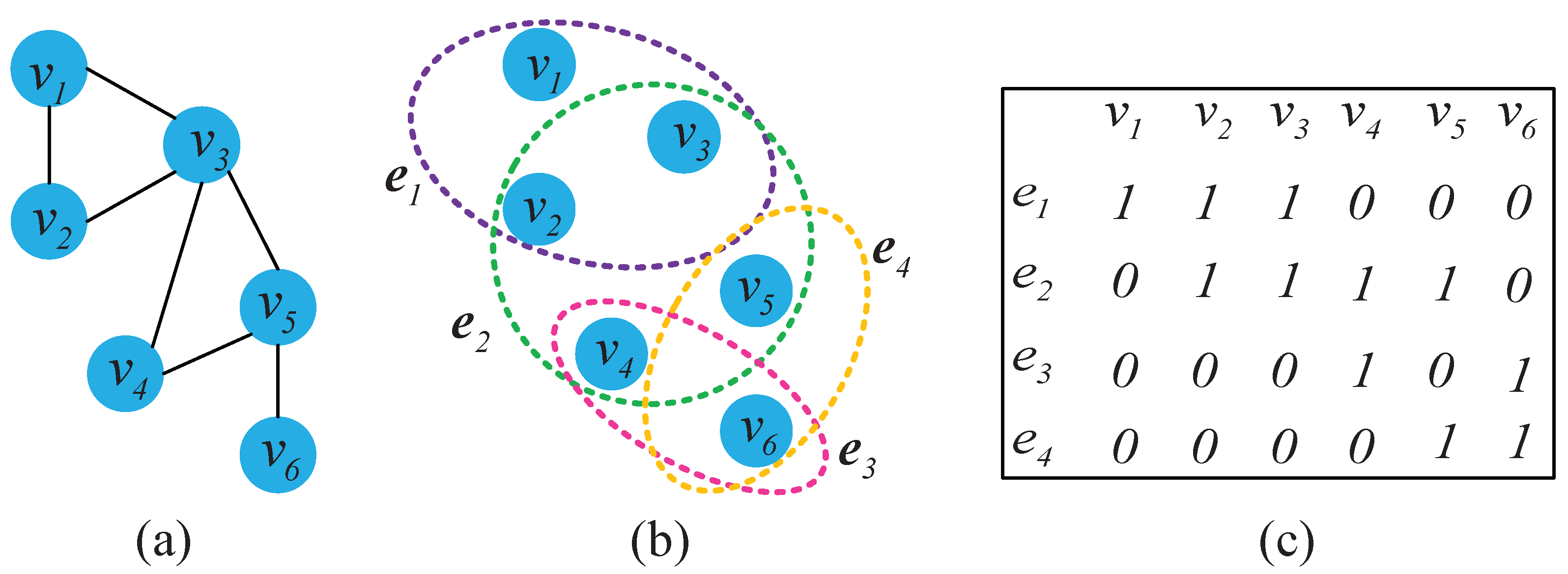
There is an example to illustrate the hypergraph in Figure 1. A vertex is denoted as a circle (such as ${\mathbf{v}}_1$, ${\mathbf{v}}_2$, ${\mathbf{v}}_5$). As shown in Figure 1a, the simple graph only holds two vertices per edge, which just describes a single one-to-one relationship (such as ${\mathbf{v}}_1$ and ${\mathbf{v}}_2$, and ${\mathbf{v}}_1$ and ${\mathbf{v}}_3$). In Figure 1b, each hyper-edge is represented by a curve (such as a hypergraph $e_1$ is constructed by ${\mathbf{v}}_1$, ${\mathbf{v}}_2$, ${\mathbf{v}}_3$), which represents complex multiple relations among pixels. That is, a hypergraph can describe the local neighborhood structure well and preserve the complex relationships within the neighborhood. This hypergraph consists of six vertices and four hyper-edges, and the corresponding incidence matrix is shown in Figure 1c. The incidence matrix intuitively represents affinity relationships between vertices and hyper-edges, the non-zero element in each row indicates that a hyper-edge is associated with the vertex, otherwise the vertex and the hyper-edge are not interrelated.

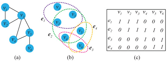
Figure 1. An example for hypergraph: (a) simple graph; (b) hypergraph; and (c) incidence matrix H.

However, the hypergraph model only represents complex higher-order relations between pixels in spectral domain, and it fails to consider spatial information in hyperspectral image that limits the discriminant ability of embedding features for land cover classification.

3. SSRHE

To reveal the complex structure in HSI, we propose a new hypergraph learning method called spatial-spectral joint regularized sparse hypergraph embedding (SSRHE) for dimensionality reduction of HSI data. At first, SSRHE constructs a regularized sparse intraclass hypergraph and a regularized sparse interclass hypergraph by exploring sparse representation (SR) and prior knowledge. After that, it exploits the spatial consistency and global structure of HSI by computing a local spatial neighborhood preserving scatter and a total scatter, which brings benefits for combining spatial structure and spectral information for DR. Finally, an optimal objective function is designed to learn a spatial-spectral discriminant projection by minimizing the regularized sparse intraclass hypergraph scatter and the local spatial neighborhood preserving scatter, while maximizing the regularized sparse interclass hypergraph scatter and the total scatter of samples simultaneously. The flowchart of the proposed SSRHE method is shown in Figure 2.

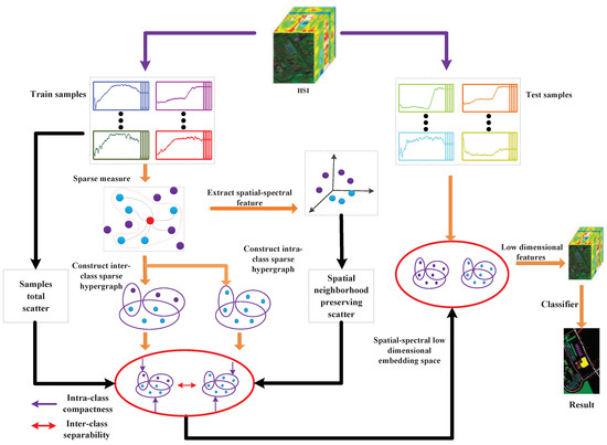
Figure 2. Flowchart of the proposed SSRHE method.

3.1. The Regularized Sparse Hypergraph Model

To discover the complex structure of HSI data, a hypergraph model is exploited to reveal the intrinsic relations between pixels. However, it remains difficult to choose a proper neighborhood size for constructing hypergraphs. Since sparse representation has natural discriminating power to adaptively reveal the inherent relationship of data [47,48,49], a sparse hypergraph model is designed based on SR theory.

Inspired by the observation that the most compact expression of a certain sample is generally given from similar samples, sparse coefficients are explored to find neighbors adaptively. Suppose $\mathbf{S}\in R^{N\times N}$ is the sparse coefficient matrix of data samples. The sparse coefficients can be calculated as follows:

$$\underset{\mathbf{S}}{min}{∥s_i∥}_{1}s.t.∥{\mathbf{x}}_i-\mathbf{X}{\mathbf{s}}_i∥\le \epsilon ,{\mathbf{s}}_i>0$$

(5)

where $\epsilon$ denotes the sparse error, ${\mathbf{s}}_i={[{\mathbf{s}}_{i,1},{\mathbf{s}}_{i,2},\dots ,{\mathbf{s}}_{i,i-1},0,{\mathbf{s}}_{i,i+1},\dots ,{\mathbf{s}}_{i,N}]}^T$ represents the sparse coefficients of pixel ${\mathbf{x}}_i$, which can be optimized by using Alternating Direction Method of Multipliers (ADMM) framework [50,51]. With the sparse coefficient matrix S, a hypergraph can be constructed with the criterion that nodes ${\mathbf{x}}_i$ and ${\mathbf{x}}_j$ are connected in a hyper-edge if sparse coefficient ${\mathbf{s}}_{ij}$ is not equal to 0. Since sparse coefficients can reflect the similarity between data, non-zero correspondence coefficient indicates the correlation between pixels, a large value indicates a high similarity. Compared with Euclidean metric, sparse coefficients can more effectively select neighbors of HSI data.

According to sparse coefficients and label information of samples, we construct a within-class sparse hypergraph ${\mathbf{G}}^w(\mathbf{X},{\mathbf{E}}_H^w,{\mathbf{W}}_H^w)$ and a between-class sparse hypergraph ${\mathbf{G}}^b(\mathbf{X},{\mathbf{E}}_H^b,{\mathbf{W}}_H^b)$ to characterize the intrinsic structure of HSI data. $\mathbf{X}$ is denoted as the vertex set, ${\mathbf{E}}_H^w$ and ${\mathbf{E}}_H^b$ are the sets of intraclass hyper-edge and interclass hyper-edge. ${\mathbf{W}}_H^w$ and ${\mathbf{W}}_H^b$ are the weight matrices of hyper-edges of ${\mathbf{G}}^w$ and ${\mathbf{G}}^b$, respectively.

In ${\mathbf{G}}^w$, the intraclass hyper-edge $e^w$ is formed by connecting pixel ${\mathbf{x}}_i$ with its corresponding neighbors whose sparse coefficients are non-zero. The subedge weights of $e^w$ and $e^b$ can be defined as

$$w_{ij}^w=\left\{\begin{array}{c}\begin{array}{cccc}\phi \ast s_{ij},& if& s_{ij}\ne 0& \begin{array}{cc}and& l_i=l_j\end{array}\end{array}\hfill \\ \begin{array}{cc}0,& others\end{array}\hfill \end{array}\right.$$

(6)

$$w_{ij}^b=\left\{\begin{array}{c}\begin{array}{cccc}{s}_{ij},& if& s_{ij}\ne 0& \begin{array}{cc}and& l_i\ne l_j\end{array}\end{array}\hfill \\ \begin{array}{cc}0,& others\end{array}\hfill \end{array}\right.$$

(7)

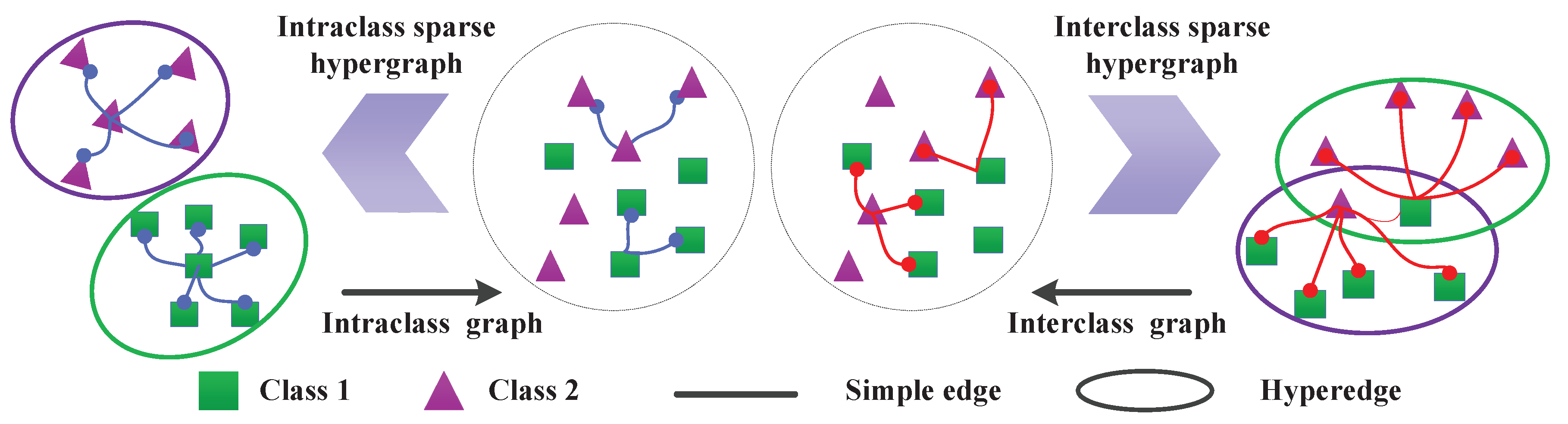
in which ${\mathbf{s}}_{ij}$ is the sparse coefficient between pixel ${\mathbf{x}}_i$ and ${\mathbf{x}}_j$ and parameter $\phi$ ($\phi >1$) is used to enhance the contribution of samples from the same class for improving the discriminant power. Figure 3 illustrates the construction of sparse hypergraph on a simple classification model. As shown in Figure 3, a simple graph considers only pairwise relation between two observed samples, while the sparse hypergraph through sparse representation can select neighbors of samples adaptively and represent complex multiple relations among HSI pixels.

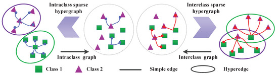
Figure 3. A simple two classification model to explain the construction of sparse hypergraph.

The weight matrices corresponding to hyper-edge regions are defined as

$${\omega }_i^w=w\left(e_i^w\right)={\sum }_{{\mathbf{x}}_j\in {e_i}^w}{w}_{ij}^w$$

(8)

$${\omega }_i^b=w\left(e_i^b\right)={\sum }_{{\mathbf{x}}_j\in {e_i}^b}{w}_{ij}^b$$

(9)

The incidence matrix ${\mathbf{H}}^w=[H_{ij}^w:h(e_j^w,{\mathbf{x}}_i)]\in R^{\left|{\mathbf{E}}^w\right|\times \left|\mathbf{X}\right|}$ of intraclass hypergraph is calculated by

$$H_{ij}^w=\left\{\begin{array}{c}\begin{array}{cccc}exp(-\frac{({\mathbf{x}}_i-{\mathbf{x}}_j){({\mathbf{x}}_i-{\mathbf{x}}_j)}^T}{2t^2}),& if& {\mathbf{x}}_i,{\mathbf{x}}_j\in e_j^w& \end{array}\hfill \\ \begin{array}{cc}0,& others\end{array}\hfill \end{array}\right.$$

(10)

where $t=\frac{1}{\mathcal{N}{\left(e_i^w\right)}^2}{\sum }_j\sqrt{({\mathbf{x}}_i-{\mathbf{x}}_j){({\mathbf{x}}_i-{\mathbf{x}}_j)}^T}$ is the heat-kernel parameter, that is the mean value of pixels in one hyper-edge, $\mathcal{N}\left(e_i\right)$ denotes the number of vertices in each hyper-edge region.

According to ${\mathbf{H}}^w$ and $w\left(e^w\right)$, the degree of vertex ${\mathbf{x}}_i\in \mathbf{X}$ and the degree of intraclass hyper-edge $e_i^w\in {\mathbf{E}}^w$ are computed by

$$\begin{array}{c}{\theta }_i^w=d({\mathbf{x}}_i,e_j^w)={\sum }_{j}w(e_j^w)h(e_j^w,{\mathbf{x}}_i)={\sum }_{j}w(e_j^w)H_{ij}^w\hfill \end{array}$$

(11)

$${\vartheta }_i^w=d\left(e_i^w\right)={\sum }_{j}h(e_i^w,x_j)={\sum }_j{H}_{ij}^w$$

(12)

For the between-class hypergraph ${\mathbf{G}}_H^b$, the between-class incidence matrix ${\mathbf{H}}^b=[H_{ij}^b:h(e_j^b,{\mathbf{x}}_i)]\in R^{\left|{\mathbf{E}}^b\right|\times \left|\mathbf{X}\right|}$ is defined as

$$H_{ij}^b=\left\{\begin{array}{c}\begin{array}{cccc}exp(-\frac{({\mathbf{x}}_i-{\mathbf{x}}_j){({\mathbf{x}}_i-{\mathbf{x}}_j)}^T}{2t^2}),& if& {\mathbf{x}}_i,{\mathbf{x}}_j\in e_j^b& \end{array}\hfill \\ \begin{array}{cc}0,& others\end{array}\hfill \end{array}\right.$$

(13)

Based on ${\mathbf{H}}^b$ and $w\left(e^b\right)$, the degree of vertex ${\mathbf{x}}_i$ and interclass hyper-edge $e_i^b$ can be defined as

$${\theta }_i^b=d({\mathbf{x}}_i,e_j^b)={\sum }_{j}w(e_j^b)h(e_j^b,{\mathbf{x}}_i)={\sum }_{j}w(e_j^b)H_{ij}^b$$

(14)

$${\vartheta }_i^b=d\left(e_i^b\right)={\sum }_{j}h(e_i^b,{\mathbf{x}}_j)={\sum }_j{H}_{ij}^b$$

(15)

In low-dimensional embedding space, the pixels from the same class should be as compact as possible for the intraclass sparse hypergraph, whereas pixels from different classes should be as separated as possible with the interclass sparse hypergraph. Therefore, the objective functions with intraclass and interclass sparse hypergraph constraint are constructed as

$$\begin{array}{c}\underset{P}{argmin}\frac{1}{2}{\sum }_{e_k^w\in E^w}{\sum }_{x_i,x_j\in e_k^w}\frac{w\left(e_k^w\right)h(e_k^w,x_i)h(e_k^w,x_j)}{d\left(e_k^w\right)}{∥P^T{x}_i-P^T{x}_j∥}^2\hfill \\ ={\sum }_{k=1}^n{\sum }_{i,j=1}^n\frac{w\left(e_k^w\right)H_{ik}^w{H}_{jk}^w}{{\vartheta }_k^w}tr(P^T{x}_i{x_i}^{T}P-P^T{x}_j{x_i}^{T}P)\hfill \\ =\left\{{\sum }_{k=1}^n{\sum }_{i=1}^n\frac{w\left(e_k^w\right)H_{ik}^w}{{\theta }_i^w}tr\left(P^T{x}_i{x_i}^{T}P\right){\sum }_{j=1}^n\frac{H_{jk}^w{\theta }_i^w}{{\vartheta }_k^w}\right\}-\left\{{\sum }_{k=1}^n{\sum }_{i,j=1}^n\frac{tr\left[P^T{x}_{j}w\left(e_k^w\right)H_{ik}^w{H}_{jk}^w{x_i}^{T}P\right]}{{\vartheta }_k^w}\right\}\hfill \\ =tr\left(P^{T}X{D}_v^w{X}^{T}P\right)-tr\left[P^{T}X{H}^w{W}^w{\left(D_e^w\right)}^{-1}{\left(H^w\right)}^T{X}^{T}P\right]\hfill \\ =tr\left\{P^{T}X[D_v^w-H^w{W}^w{\left(D_e^w\right)}^{-1}{\left(H^w\right)}^T]X^{T}P\right\}\hfill \\ =\mathrm{t}r\left(P^{T}X{L}^w{X}^{T}P\right)\hfill \end{array}$$

(16)

$$\begin{array}{c}\underset{P}{argmax}\frac{1}{2}{\sum }_{e_k^b\in E^b}{\sum }_{x_i,x_j\in e_k^b}\frac{w\left(e_k^b\right)h(e_k^b,x_i)h(e_k^b,x_j)}{d\left(e_k^b\right)}{∥P^T{x}_i-P^T{x}_j∥}^2\hfill \\ ={\sum }_{k=1}^n{\sum }_{i,j=1}^n\frac{w\left(e_k^b\right)H_{ik}^b{H}_{jk}^b}{{\vartheta }_k^b}tr(P^T{x}_i{x_i}^{T}P-P^T{x}_j{x_i}^{T}P)\hfill \\ =\left\{{\sum }_{k=1}^n{\sum }_{i=1}^n\frac{w\left(e_k^b\right)H_{ik}^b}{{\theta }_i^b}tr\left(P^T{x}_i{x_i}^{T}P\right){\sum }_{j=1}^n\frac{H_{jk}^b{\theta }_i^b}{{\vartheta }_k^b}\right\}-\left\{{\sum }_{k=1}^n{\sum }_{i,j=1}^n\frac{tr\left[P^T{x}_{j}w\left(e_k^b\right)H_{ik}^b{H}_{jk}^b{x_i}^{T}P\right]}{{\vartheta }_k^b}\right\}\hfill \\ =tr\left(P^{T}X{D}_v^b{X}^{T}P\right)-tr\left[P^{T}X{H}^b{W}^b{\left(D_e^b\right)}^{-1}{\left(H^b\right)}^T{X}^{T}P\right]\hfill \\ =tr\left\{P^{T}X[D_v^b-H^b{W}^b{\left(D_e^b\right)}^{-1}{\left(H^b\right)}^T]X^{T}P\right\}\hfill \\ =\mathrm{t}r\left(P^{T}X{L}^b{X}^{T}P\right)\hfill \end{array}$$

(17)

where ${\mathbf{L}}^w={\mathbf{D}}_v^w-{\mathbf{H}}^w{\mathbf{W}}^w{\left({\mathbf{D}}_e^w\right)}^{-1}{\left({\mathbf{H}}^w\right)}^T$ is the intraclass sparse hypergraph Laplacian matrix and ${\mathbf{L}}^b={\mathbf{D}}_v^b-{\mathbf{H}}^b{\mathbf{W}}^b{\left({\mathbf{D}}_e^b\right)}^{-1}{\left({\mathbf{H}}^b\right)}^T$ denotes the interclass sparse hypergraph Laplacian matrix. ${\mathbf{D}}_v^w$, ${\mathbf{D}}_v^b$, ${\mathbf{D}}_e^w$, ${\mathbf{D}}_e^b$, ${\mathbf{W}}^w$, ${\mathbf{W}}^b$ with respect to ${\theta }^w$, ${\theta }^b$, ${\vartheta }^w$, ${\vartheta }^b$, $w^w$, $w^b$ can be indicated as

$${\mathbf{D}}_v^w=diag\left([{\theta }_1^w,{\theta }_2^w,\dots ,{\theta }_{N-1}^w,{\theta }_N^w]\right)$$

(18)

$${\mathbf{D}}_v^b=diag\left([{\theta }_1^b,{\theta }_2^b,\dots ,{\theta }_{N-1}^b,{\theta }_N^b]\right)$$

(19)

$${\mathbf{D}}_e^w=diag\left([{\vartheta }_1^w,{\vartheta }_2^w,\dots ,{\vartheta }_{N-1}^w,{\vartheta }_N^w]\right)$$

(20)

$${\mathbf{D}}_e^b=diag\left([{\vartheta }_1^b,{\vartheta }_2^b,\dots ,{\vartheta }_{N-1}^b,{\vartheta }_N^b]\right)$$

(21)

$${\mathbf{W}}^w=diag\left([{\omega }_1^w,{\omega }_2^w,\dots ,{\omega }_{N-1}^w,{\omega }_N^w]\right)$$

(22)

$${\mathbf{W}}^b=diag\left([{\omega }_1^b,{\omega }_2^b,\dots ,{\omega }_{N-1}^b,{\omega }_N^b]\right)$$

(23)

Let ${\mathbf{M}}^b=\mathbf{X}{\mathbf{L}}^b{\mathbf{X}}^T$ represent the between-class scatter of ${\mathbf{G}}^b$. ${\mathbf{M}}^w=\mathbf{X}{\mathbf{L}}^w{\mathbf{X}}^T$ is the within-class scatter of ${\mathbf{G}}^w$. Then, the mapping matrix $\mathbf{P}$ can be obtained through dealing with the following optimization problem:

$$arg\underset{\mathbf{P}}{max}\frac{tr\left({\mathbf{P}}^T{\mathbf{M}}^b\mathbf{P}\right)}{tr\left({\mathbf{P}}^T{\mathbf{M}}^w\mathbf{P}\right)}$$

(24)

In real applications, to avoid the singularity in the case of small samples, the above optimal objection can be further extended as

$$arg\underset{\mathbf{P}}{max}\frac{tr\left\{{\mathbf{P}}^T[(1-\beta ){\mathbf{M}}^b+\beta \mathbf{X}{\mathbf{X}}^T]\mathbf{P}\right\}}{tr\left\{{\mathbf{P}}^T[(1-\beta ){\mathbf{M}}^w+\beta \left(diag\left(diag\left({\mathbf{M}}^w\right)\right)\right)]\mathbf{P}\right\}}$$

(25)

where $\beta$ is a tradeoff parameter. The regularization term $\mathbf{X}{\mathbf{X}}^T$ is the maximal data variance, which is used to ensure that the diversity of HSI pixels. The diagonal regularization ${\mathbf{M}}^w$ is introduced for overcoming the singularity problem when the number of training samples is small. With regularization, Equation (25) becomes more stable to effectively reserve the useful discriminant information.

3.2. Spatial-Spectral Hypergraph Embedding

Due to the spatial consistency of HSI, the pixels in HSI are usually spatially related, which means the pixels within a small neighborhood usually possess the spatial distribution consistency of ground objects. Therefore, neighborhood pixels can be utilized to learn spatial-spectral combined features.

Suppose that pixel ${\mathbf{x}}_i$ is the center pixel, and T is the spatial neighborhood window. $(u_i,v_i)$ is the spatial coordinate of pixel ${\mathbf{x}}_i$ in the image, and the spatial neighborhood set $\mathsf{\Omega }\left({\mathbf{x}}_i\right)$ with the window size T (positive odd) can be recorded as

$$\mathsf{\Omega }\left({\mathbf{x}}_i\right)=\left\{{\mathbf{x}}_{im}:\left(u_m,v_m\right)\left|\begin{array}{c}{u}_m\in \left(u-z,v+z\right)\\ v_m\in \left(u-z,v+z\right)\end{array}\right.\right\}$$

(26)

where $z=(T-1)/\phantom{(T-1)2}2$, ${\mathbf{x}}_{im}:\left(u_m,v_m\right)$ corresponds to the m-th pixel in the spatial neighborhood. $\mathsf{\Omega }\left({\mathbf{x}}_i\right)$ has a total of $T\times T$ pixels. Thus, the distance measure in the spatial neighborhood block can be defined as

$$a_i={\sum }_{m=1}^{T^2}{∥{\mathbf{x}}_i-{\mathbf{x}}_{im}∥}^2{v}_m$$

(27)

where $v_m=exp\left\{-{∥{\mathbf{x}}_i-{\mathbf{x}}_{im}∥}^2/2{(\frac{1}{T\times T}{\displaystyle \sum _{m=1}^{T^2}}{\mathbf{x}}_{im})}^2\right\}$, which measures similarity between central pixel ${\mathbf{x}}_i$ and its spectral-spatial neighbors. For all training samples in HSI data, the local spatial neighborhood preserving scatter matrix is calculated as follows:

$${\mathbf{S}}^w={\sum }_i{a}_i={\sum }_i{{\sum }_{m=1}^{T^2}∥{\mathbf{x}}_i-{\mathbf{x}}_{im}∥}^2{v}_m={\sum }_{i=1}^N{\sum }_{m=1}^{T^2}({\mathbf{x}}_i-{\mathbf{x}}_{im}){({\mathbf{x}}_i-{\mathbf{x}}_{im})}^T{v}_m$$

(28)

To preserve the global structure of samples, a total scatter matrix is defined as

$${\mathbf{S}}^b={\sum }_{i=1}^N({\mathbf{x}}_i-\overline{\mathbf{x}}){({\mathbf{x}}_i-\overline{\mathbf{x}})}^T$$

(29)

where $\overline{\mathbf{x}}$ is the mean of all samples.

To extract low-dimensional spatial-spectral joint features, a objective function should be designed to preserve the local neighborhood as well as compact the samples with interclass hypergraph and separate the samples with interclass hypergraph simultaneously. Therefore, Equations (25), (28), and (29) are transformed into the following optimization function:

$$\left\{\begin{array}{c}\underset{\mathbf{P}}{argmax}tr\left\{\alpha {\mathbf{P}}^T\left[(1-\beta ){\mathbf{M}}^b+\beta \mathbf{X}{\mathbf{X}}^T\right]\mathbf{P}+(1-\alpha ){\mathbf{P}}^T{\mathbf{S}}^{b}P\right\}\hfill \\ \underset{\mathbf{P}}{argmin}tr\left\{\alpha {\mathbf{P}}^T\left[(1-\beta ){\mathbf{M}}^w+\beta diag\left(diag\left({\mathbf{M}}^w\right)\right)\right]\mathbf{P}+(1-\alpha ){\mathbf{P}}^T{\mathbf{S}}^w\mathbf{P}\right\}\hfill \end{array}\right.$$

(30)

The above optimal function can be further simplified as

$$\underset{\mathbf{P}}{argmax}\frac{tr\left\{\alpha {\mathbf{P}}^T\left[(1-\beta ){\mathbf{M}}^b+\beta \mathbf{X}{\mathbf{X}}^T\right]\mathbf{P}+(1-\alpha ){\mathbf{P}}^T{\mathbf{S}}^b\mathbf{P}\right\}}{tr\left\{\alpha {\mathbf{P}}^T\left[(1-\beta ){\mathbf{M}}^w+\beta diag\left(diag\left({\mathbf{M}}^w\right)\right)\right]\mathbf{P}+(1-\alpha ){\mathbf{P}}^T{\mathbf{S}}^w\mathbf{P}\right\}}$$

(31)

According to Lagrange multiplier method, Equation (31) can be solved by

$$\begin{array}{c}\left\{\alpha \left[(1-\beta ){\mathbf{M}}^b+\beta \mathbf{X}{\mathbf{X}}^T\right]+(1-\alpha ){\mathbf{S}}^b\right\}\mathbf{P}=\lambda \left\{\alpha \left[(1-\beta ){\mathbf{M}}^w+\beta diag\left(diag\left({\mathbf{M}}^w\right)\right)\right]+(1-\alpha ){\mathbf{S}}^w\right\}\mathbf{P}\hfill \end{array}$$

(32)

where $\lambda$ is an eigenvalue set. With the d largest eigenvalues corresponding eigenvector, the optimal projection matrix can be denoted as $\mathbf{P}=[{\mathbf{p}}_1,{\mathbf{p}}_2,\cdots ,{\mathbf{p}}_d]$. In the low-dimensional embedded space, the spatial-spectral embedding of test sample ${\mathbf{x}}_t$ can be given as follows:

$${\mathbf{y}}_t={\mathbf{P}}^T{\mathbf{x}}_t$$

(33)

In summary, SSRHE compacts the samples from the same class and spatial neighborhood while separates interclass samples, and the embedding features possess stronger discriminative power that ensures good classification performance. The steps of the proposed SSRHE method are shown in Algorithm 1.

Algorithm 1 SSRHE.

Input: HSI dataset $\mathbf{X}=[{\mathbf{x}}_1,{\mathbf{x}}_2,\cdots ,{\mathbf{x}}_N]\in R^{D\times N}$, corresponding class label set $\mathbf{L}$, tradeoff parameters $\alpha$, $\beta$, weighted coefficient $\phi$, spatial neighborhood size T, reduced dimensionality d. 1: According to ADMM, compute sparse coefficient matrix $\mathbf{S}$; 2: Compute the weights of intraclass and interclass hyperedge by Equations (8) and (9); 3: Compute the intraclass hyper-Laplacian matrix: ${\mathbf{L}}^w={\mathbf{D}}_v^w-{\mathbf{H}}^w{\mathbf{W}}^w{\left({\mathbf{D}}_e^w\right)}^{-1}{\left({\mathbf{H}}^w\right)}^T$; 4: Compute the interclass hyper-Laplacian matrix: ${\mathbf{L}}^b={\mathbf{D}}_v^b-{\mathbf{H}}^b{\mathbf{W}}^b{\left({\mathbf{D}}_e^b\right)}^{-1}{\left({\mathbf{H}}^b\right)}^T$; 5: Compute the local spatial neighborhood preserving scatter matrix: 6:    ${\mathbf{S}}^w={\sum }_i{a}_i={\sum }_i{{\sum }_{m=1}^{T^2}∥{\mathbf{x}}_i-{\mathbf{x}}_{im}∥}^2{v}_m={\sum }_{i=1}^N{\sum }_{m=1}^{T^2}({\mathbf{x}}_i-{\mathbf{x}}_{im}){({\mathbf{x}}_i-{\mathbf{x}}_{im})}^T{v}_m$ 7: Compute the extended total scatter matrix: ${\mathbf{S}}^b={\sum }_{i=1}^N({\mathbf{x}}_i-\overline{\mathbf{x}}){({\mathbf{x}}_i-\overline{\mathbf{x}})}^T$; 8: Solve the generalized eigenvalue problem: 9:    $\left\{\alpha \left[(1-\beta ){\mathbf{M}}^b+\beta \mathbf{X}{\mathbf{X}}^T\right]+(1-\alpha ){\mathbf{S}}^b\right\}\mathbf{P}=\lambda \left\{\alpha \left[(1-\beta ){\mathbf{M}}^w+\beta diag\left(diag\left({\mathbf{M}}^w\right)\right)\right]+(1-\alpha ){\mathbf{S}}^w\right\}\mathbf{P}$ 10: Obtain the optimal projection matrix with largest eigenvalues corresponding eigenvectors: 11:    $\mathbf{P}=[{\mathbf{p}}_1,{\mathbf{p}}_2,\cdots ,{\mathbf{p}}_d]$ Output: 12: Low-dimensional spatial-spectral embedding features of test samples:$\mathbf{Y}={\mathbf{P}}^T\mathbf{X}$

In this paper, we adopt big O notation to analyze the computational complexity of SSRHE. Spatial neighborhood size and the number of sparse iterations are denoted as T and t, respectively. The sparse coefficient matrix $\mathbf{S}$ is computed with the cost of $O\left(Nt\right)$. The weight of intraclass hyperedge and the weight of interclass hyperedge both take $O\left(N^2\right)$. The intraclass incidence matrix ${\mathbf{H}}^{\mathbf{w}}$ and the interclass incidence matrix ${\mathbf{H}}^{\mathbf{b}}$ are both calculated with $O\left(N^2\right)$. The cost of diagonal matrices ${\mathbf{W}}^{\mathbf{w}}$, ${\mathbf{W}}^{\mathbf{b}}$, ${\mathbf{D}}_{\mathbf{v}}^{\mathbf{w}}$, ${\mathbf{D}}_{\mathbf{v}}^{\mathbf{b}}$, ${\mathbf{D}}_{\mathbf{e}}^{\mathbf{w}}$, and ${\mathbf{D}}_{\mathbf{e}}^{\mathbf{b}}$ are $O\left(8N\right)$). The intraclass hyper-Laplacian matrix ${\mathbf{L}}^{\mathbf{w}}$ and the interclass hyper-Laplacian matrix ${\mathbf{L}}^{\mathbf{b}}$ both cost $O\left(N^3\right)$. The local spatial neighborhood preserving scatter matrix ${\mathbf{S}}^{\mathbf{w}}$ takes $O\left(DN{T}^2\right)$. The extended total scatter matrix ${\mathbf{S}}^{\mathbf{b}}$ costs $O\left(DN\right)$. The costs of matrix ${\mathbf{M}}^{\mathbf{w}}$ and ${\mathbf{M}}^{\mathbf{b}}$ are both $O\left(D{N}^2\right)$. $\mathbf{X}{\mathbf{X}}^{\mathbf{T}}$ costs $O\left(DN\right)$. It takes $O\left(D^3\right)$ to deal with the generalized problem of Equation (32). The total time complexity of SSRHE is $O\left(D^3+D{N}^2+N^3\right)$.

4. Experimental Results and Discussion

Some experiments were performed on two real HSI datasets to verity the effectiveness of the proposed method, and several state-of-the-art DR methods were compared with SSRHE in the experiments.

4.1. HSI Datasets

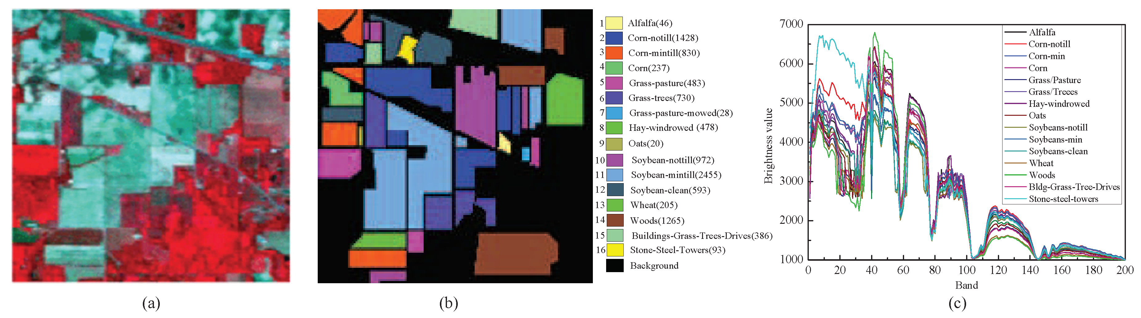
Indian Pines Dataset: This hyperspectral image is a scene of northwest Indiana collected by an airborne imaging spectrometer sensor in 1992. It consists of $145\times 145$ pixels and 220 spectral bands that cover the wavelength from 400 to 2450 nm. After removing the noise and water absorption bands, 200 spectral bands remained for use in the experiments. This image contains total 16 land cover types. The dataset in false color and its corresponding ground truth map are shown in Figure 4.

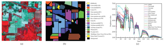
Figure 4. Indian Pines hyperspectral image: (a) HSI in false color; (b) ground truth; and (c) spectral curve. (Note that the number of samples for each class is shown in brackets.)

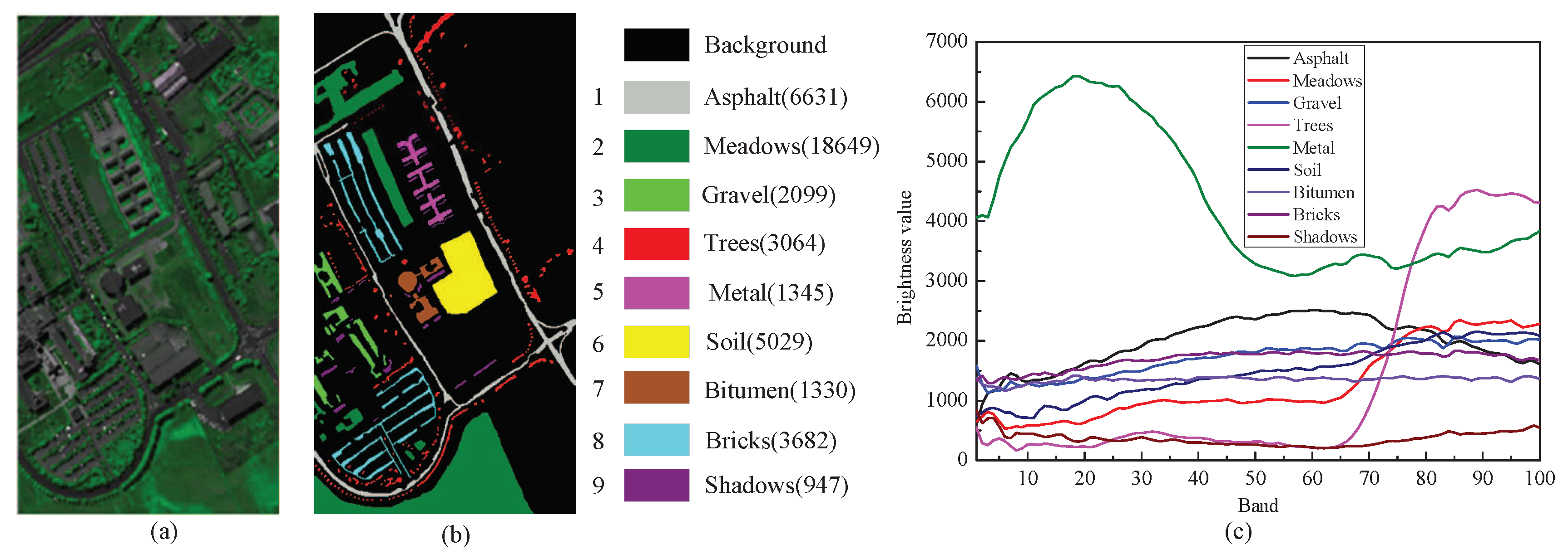
University of Pavia (PaviaU) Dataset: This hyperspectral image covering the area of Pavia University in northern Italy was collected by ROSIS sensor in 2002. The spatial size of this image is $640\times 340$ pixels and the number of spectral band is 115. Due to the atmospheric affection, 12 bands were discarded and the remaining 103 spectral bands were used for experiment. The false color and ground truth map for this scene are shown in Figure 5.

Figure 5. PaviaU hyperspectral image: (a) HSI in false color; (b) ground truth; and (c) spectral curve. (Note that the number of samples for each class is shown in brackets.)

4.2. Experimental Setup

In experiments, each HSI dataset was randomly divided into training and test sets. The training samples were utilized to learn a feature extracted model to obtain their low-dimensional embedding features. After that, the classifier was applied to obtain the class labels of test samples. The overall classification accuracy (OA), average classification accuracy of each class (AA), and kappa coefficient (KC) were employed to evaluate classification results.

To demonstrate the effectiveness of the proposed method, we compared SSRHE with four spectral-based approaches, LPP, LDA, MFA, and RLDE; two spatial-spectral combined approaches, LPNPE and SSCE; and a hypergraph method, DHLP. For all approaches, we tuned the parameters by cross-validation to achieve good results. In LPNPE, the size of spatial-spectral window was set to 15 for the PaviaU data and 11 for the Indian Pines data. In SSCE, the window scale and the local neighbor size were both set to 5 on both datasets. For RLDE and MFA, the intraclass neighbor size was set to 3 and 8, while the interclass neighbor size was set to 5 and 60, respectively. The number of nearest neighbor in DHLP was selected as 9.

The nearest neighbor (1-NN) classifier was applied for classification. Each experiment was randomly repeated ten times. All experiments were performed on a personal computer with i5-4590 central processing unit, 8-G memory, and 64-bit Windows 7 using MATLAB 2014a.

4.3. Parameters Selection

For the proposed SSRHE algorithm, there are four important parameters: spatial neighborhood size T, weighted coefficient $\phi$, tradeoff parameters $\alpha$ and $\beta$. To select the optimal parameters, we performed some parameters selection experiments on the Indian Pines and PaviaU datasets. In each experiment, we randomly selected five samples from each class as training set and the remaining samples were used for testing.

To explore the effect of tradeoff parameters $\alpha$ and $\beta$, we turned them with a set of $\{0,0.01,0.05,0.1,0.2,\cdots ,0.9,1\}$. Figure 6 and Figure 7 show the classification accuracies with respect to $\alpha$ and $\beta$ on two datasets. As shown in Figure 6, an increasing $\alpha$ produced subtle change of OAs under a fixed $\beta$. The OAs first varied slightly and then declined significantly with the increase of $\alpha$ on Indian Pines dataset, since a too large $\alpha$ led to the algorithm losing the property of spatial-domain in HSI and the obtained features might fail to represent the intrinsic structure of hyperspectral image. For PaviaU dataset, the OAs first increased with increasing $\alpha$ and $\beta$, and then tended to decline. To balance the influence of spectral and spatial information for classification, we set parameters $\alpha =0.3$ and $\beta =0.7$ for the Indian Pines dataset, and $\alpha =0.2$ and $\beta =0.5$ for PaviaU dataset based on the results presented in Figure 6 and Figure 7.

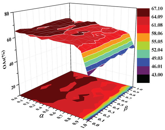
Figure 6. The OAs of SSRHE with different $\alpha$ and $\beta$ on Indian Pines dataset.

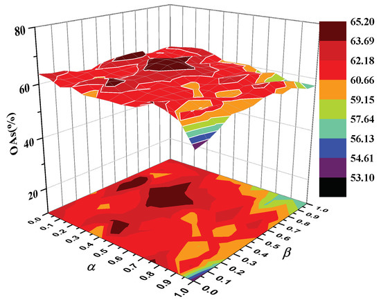
Figure 7. The OAs of SSRHE with different $\alpha$ and $\beta$ on PaviaU dataset.

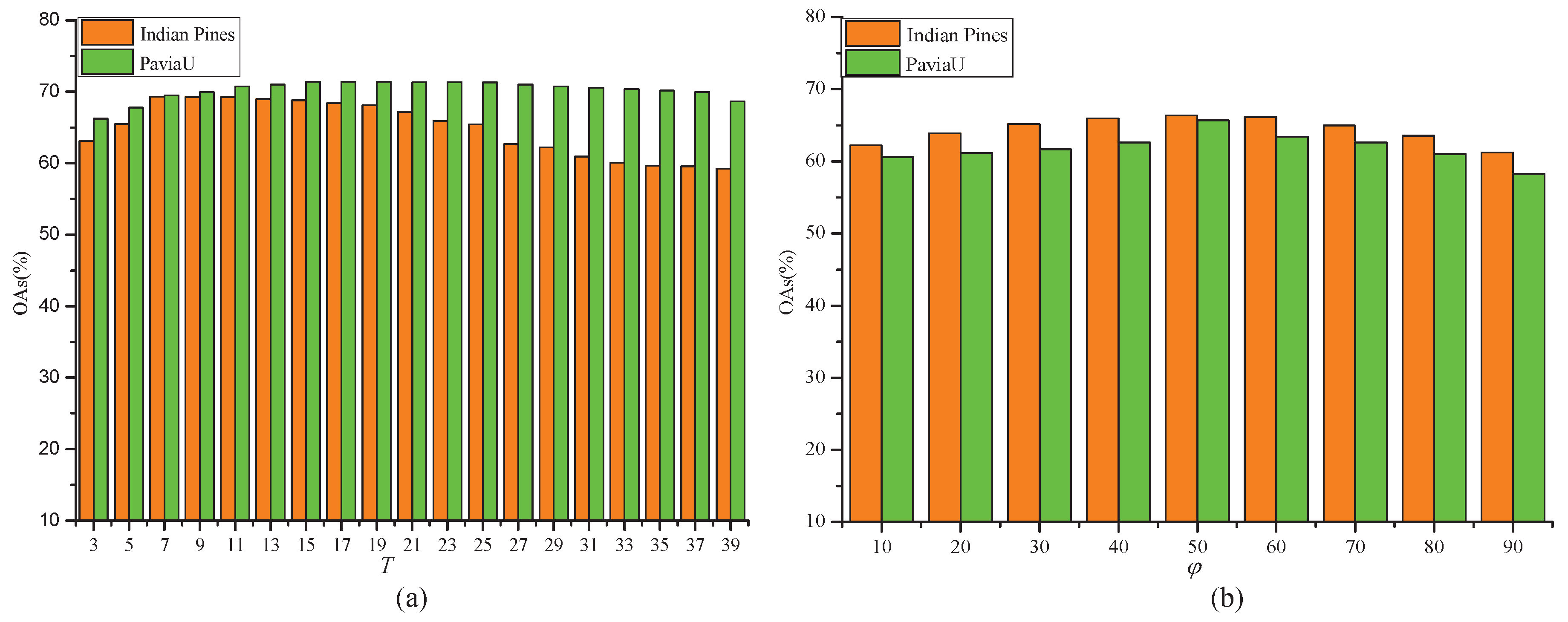
The parameters T and $\phi$ have a significant influence on the discrimination of SSRHE. The former is defined to determine the size of spatial neighborhood and the latter is exploited to adjust the compactness of the interclass neighbors. To analyze the influence of two parameters for SSRHE, we performed two experiments with respect to T and $\phi$, and the corresponding experimental results on two HSI datasets are shown in Figure 8. In Figure 8a, it is clear that the OAs first quickly increased with the growth of T on two dataset because a larger spatial neighborhood was beneficial to preserving more useful spatial-domain information in HSI. However, if the value of T was too large, it might bring pixels from other classes into training model, as well as greatly increase computational complexity. According to the results in Figure 8a, the size of spatial neighborhood T was set to 7 for Indian Pines dataset and 15 for PaviaU dataset. As shown in Figure 8b, with the increasing of $\phi$, the OAs improved until reaching a peak value due to further enhancing the compactness of intraclass samples in the embedding space. While $\phi$ kept increasing, the OAs declined since too large $\phi$ weakened the ability to extract between-class features. Therefore, we set $\phi =50$ for the Indian Pines dataset and $\phi =60$ for the PaviaU dataset.

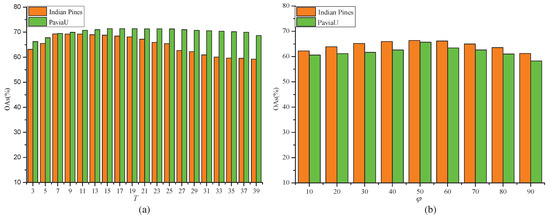
Figure 8. OAs with respect to parameters T and $\phi$ on different datasets: (a) the OAs of T; and (b) the OAs of $\phi$.

4.4. Investigation of Embedding Dimension

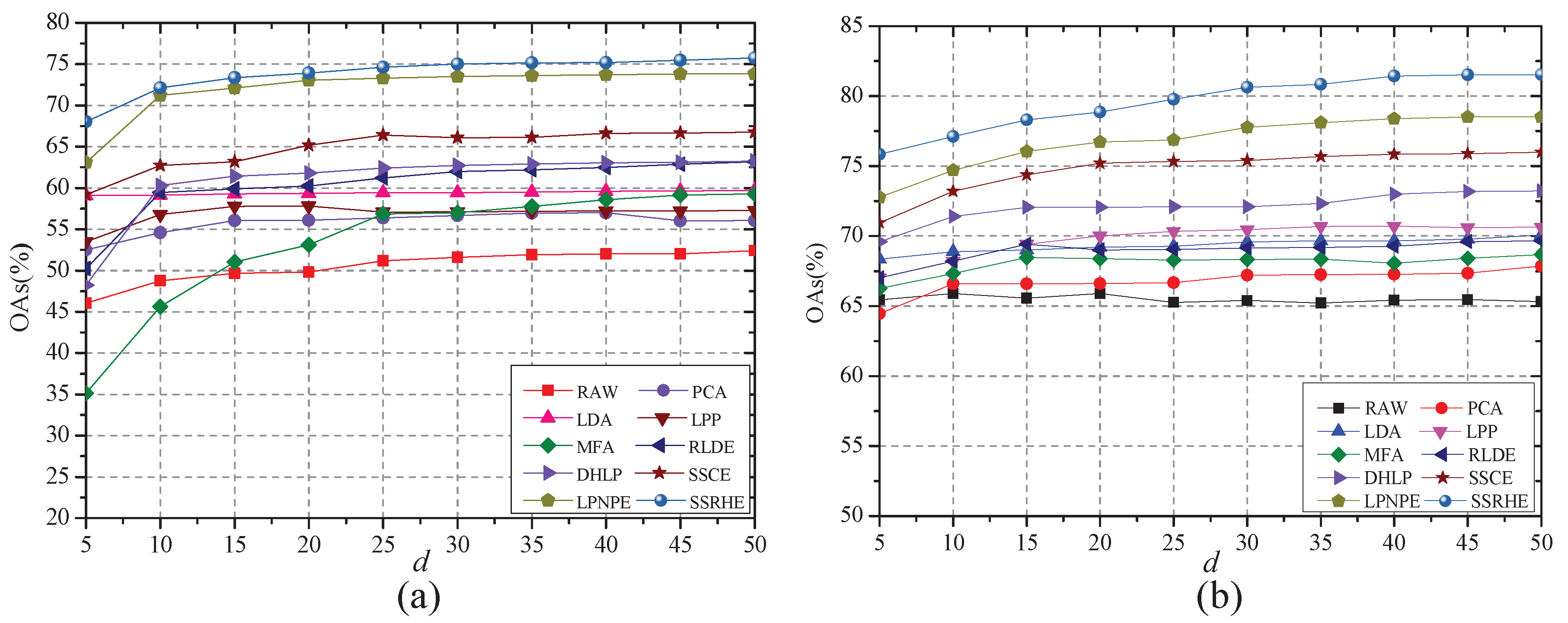
To explore how the embedding dimension d affects the performance of the proposed SSRHE method, thirty samples were randomly selected from each class for training, and d was tuned from 5 to 50 with an interval of 5. Figure 9 shows the classification accuracy of SSRHE and other DR methods with different embedding dimensions on Indian Pines and PaviaU datasets. According to Figure 9, the OAs firstly rapidly rose and then tended to stabilize with an increasing d, because embedding features with high dimension contained more useful information for training, while too large dimension might lead to information saturation. The classification accuracies of the most DR methods were better than the RAW method since these methods can remove the redundant information in HSI. The proposed SSRHE achieved the best classification performance in comparison with other methods on two HSI datasets. The reason is that SSRHE discovered the complex relationships between samples by hypergraph model and fused the useful spatial information for extracting discriminant features for classification.

Figure 9. OAs with different embedding d: (a) Indian Pines dataset; anf (b) Pavia U dataset.

4.5. Investigation of Classification Performance

To evaluate the performance of the proposed method under different training conditions, we selected $n_i\left(n_i=5,20,50,100,200\right)$ samples per class for training, and 1-NN classifier was utilized to classify the remaining samples. Each experiment was repeated ten times, the averaged OA with standard deviations (STDs) and kappa coefficient (KC) of all DR methods on Indian Pines and PaviaU datasets are shown in Table 1 and Table 2.

Table 1. Classification results using different methods with different classifiers for the Indian pines dataset. (OA ± STDs (%) (KC)).

Method	5	20	50	100	200
RAW	43.6 ± 2.8 (0.372)	54.9 ± 1.7 (0.495)	60.1 ± 1.4 (0.552)	63.6 ± 0.9 (0.588)	66.9 ± 0.6 (0.622)
PCA	43.4 ± 2.7 (0.370)	54.9 ± 1.6 (0.495)	60.2 ± 1.2 (0.553)	63.9 ± 0.8 (0.591)	67.0 ± 0.6 (0.622)
LDA	32.5 ± 4.8 (0.253)	51.6 ± 1.9 (0.459)	64.4 ± 1.2 (0.599)	71.0 ± 0.5 (0.672)	74.4 ± 0.7 (0.706)
LPP	43.6 ± 3.7 (0.372)	54.5 ± 1.8 (0.491)	59.7 ± 1.2 (0.546)	62.7 ± 1.0 (0.578)	65.8 ± 0.5 (0.609)
MFA	44.1 ± 4.0 (0.377)	57.1 ± 1.6 (0.520)	66.8 ± 1.9 (0.625)	70.8 ± 1.1 (0.669)	72.0 ± 1.0 (0.680)
RLDE	41.7 ± 1.1 (0.622)	60.9 ± 1.5 (0.561)	69.8 ± 1.4 (0.659)	74.6 ± 0.7 (0.711)	78.4 ± 0.6 (0.751)
DHLP	44.1 ± 3.8 (0.377)	57.2 ± 2.1 (0.522)	68.9 ± 1.2 (0.649)	73.8 ± 0.8 (0.702)	77.6 ± 0.7 (0.741)
SSCE	30.2 ± 4.5 (0.230)	69.7 ± 1.0 (0.658)	76.3 ± 0.9 (0.730)	79.1 ± 0.5 (0.760)	82.9 ± 0.6 (0.801)
LPNPE	60.2 ± 3.5 (0.594)	74.0 ± 1.4 (0.706)	79.3 ± 0.7 (0.759)	81.6 ± 0.6 (0.791)	84.2 ± 0.6 (0.817)
SSRHE	65.6 ± 2.3 (0.615)	74.8 ± 1.2 (0.711)	80.0 ± 1.0 (0.765)	82.9 ± 1.0 (0.803)	86.7 ± 1.0 (0.829)

Note that the best results of a row are marked in bold.

Table 2. Classification results using different methods with different classifiers for the PaviaU dataset. (OA ± STDs (%) (KC)).

Method	5	20	50	100	200
RAW	60.5 ± 4.2 (0.512)	66.4 ± 2.4 (0.583)	73.5 ± 1.6 (0.663)	76.4 ± 0.8 (0.698)	78.8 ± 0.8 (0.724)
PCA	60.5 ± 4.2 (0.512)	66.5 ± 2.2 (0.583)	73.4 ± 1.6 (0.662)	76.4 ± 0.8 (0.697)	78.7 ± 0.6 (0.724)
LDA	46.7 ± 6.4 (0.351)	59.6 ± 1.8 (0.495)	73.5 ± 1.4 (0.662)	78.9 ± 0.9 (0.727)	83.4 ± 0.6 (0.782)
LPP	47.0 ± 5.6 (0.354)	59.3 ± 2.6 (0.500)	72.8 ± 2.3 (0.654)	78.3 ± 1.3 (0.722)	82.2 ± 1.2 (0.768)
MFA	64.5 ± 4.3 (0.555)	69.2 ± 4.5 (0.613)	76.4 ± 2.0 (0.699)	78.1 ± 2.4 (0.715)	79.1 ± 2.2 (0.730)
RLDE	64.4 ± 3.2 (0.555)	74.6 ± 2.7 (0.677)	77.9 ± 2.2 (0.718)	82.1 ± 1.0 (0.770)	84.8 ± 1.0 (0.802)
DHLP	56.8 ± 8.0 (0.471)	62.2 ± 3.6 (0.530)	70.8 ± 2.1 (0.629)	77.5 ± 2.7 (0.711)	80.2 ± 1.5 (0.742)
SSCE	42.3 ± 5.3 (0.309)	63.3 ± 2.9 (0.543)	75.8 ± 1.7 (0.692)	82.7 ± 1.2 (0.804)	87.0 ± 0.8 (0.828)
LPNPE	68.0 ± 4.2 (0.606)	80.0 ± 2.2 (0.747)	86.3 ± 1.3 (0.822)	87.9 ± 0.9 (0.842)	89.9 ± 0.6 (0.877)
SSRHE	71.6 ± 2.7 (0.646)	82.6 ± 2.3 (0.776)	87.5 ± 1.1 (0.837)	90.0 ± 1.5 (0.882)	92.2 ± 0.2 (0.908)

Note that the best results of a row are marked in bold.

As shown in Table 1 and Table 2, for all methods, the OA and KC greatly improved and the STDs decreased with the increasing of training samples, because a large number of training samples usually provide more useful information for training. The spatial-spectral combined methods, SSCE, LPNPE and SSRHE, produced better classification results than the spectral-based methods, because they exploit the spatial and spectral information in HSI to improve the representation ability of extracted features. Among these spectral-based methods, DHLP presented better classification performance under most training conditions, since it applies the hypergraph learning model to discover the intrinsic complex relationship between samples. Compared with all the other methods, SSRHE had better discriminant performance with different proportions of training samples on two HSI datasets, especially with small size of training set. SSRHE utilizes the hypergraph framework to discover the complex multivariate relationships between interclass samples and intraclass samples, and computes two spatial neighborhood scatters to reveal the spatial correlation between each pixels in HSI, which further enhances the discriminating power of low-dimensional features.

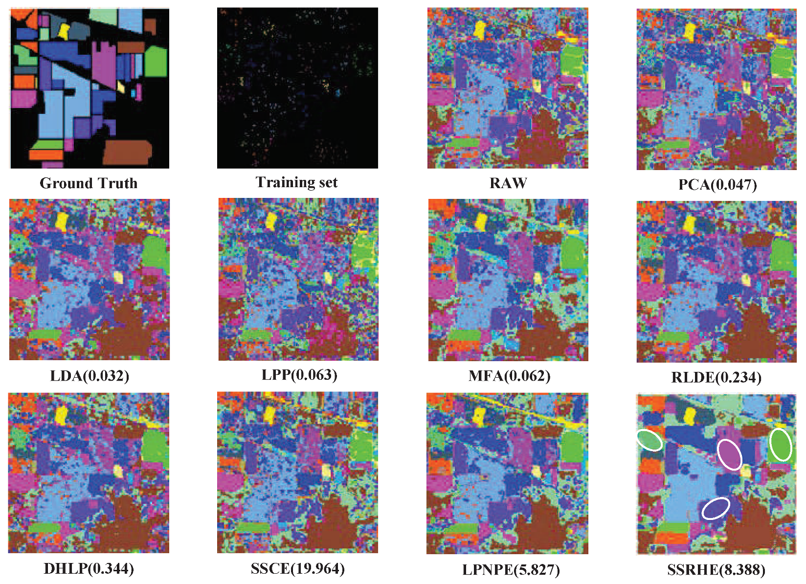
To explore the classification accuracy of the proposed method for each class, we randomly selected a percentage of samples from each class as the training set while the remaining samples were used for testing. In experiments, we set the training percent to 3% for the Indian Pines dataset and 5% for PaviaU dataset. Table 3 and Table 4 show the classification results of different DR methods on Indian Pines and PaviaU datasets, and the corresponding classification maps are displayed in Figure 10 and Figure 11.

Table 3. Classification results of different classifiers on the Indian Pines dataset.

Class	Train	Test	RAW	PCA	LDA	LPP	MFA	RLDE	DHLP	SSCE	LPNPE	SSRHE
1	10	36	41.67	41.67	77.78	36.11	50.00	61.11	63.89	55.56	77.78	94.44
2	143	1285	53.39	52.45	64.12	51.05	56.03	72.14	66.69	60.31	80.78	88.17
3	83	747	57.30	55.29	57.70	47.12	50.07	61.58	61.58	63.45	74.30	80.46
4	24	213	41.78	44.60	52.58	43.19	21.60	58.69	59.15	51.17	77.00	84.04
5	48	435	78.85	78.62	89.43	77.93	78.85	86.90	87.82	80.46	91.72	96.55
6	73	657	90.26	89.50	95.74	91.02	94.67	95.28	95.89	94.52	96.04	97.02
7	10	18	77.78	88.89	100	88.89	77.78	94.44	94.44	100	94.44	100
8	48	430	95.58	95.58	99.53	93.95	93.26	99.30	99.77	92.56	99.53	98.60
9	10	10	70.00	70.00	60.00	50.00	70.00	80.00	90.00	90.00	100	80.00
10	97	875	61.03	60.46	60.91	57.49	42.06	68.91	63.20	72.11	82.74	83.89
11	246	2209	69.76	69.85	71.89	69.62	58.85	79.36	79.22	74.02	85.92	89.50
12	59	534	39.33	37.45	65.36	32.02	47.38	67.42	62.73	50.56	87.83	83.71
13	21	184	88.04	88.04	97.83	88.04	94.57	97.28	98.37	94.57	98.91	100
14	127	1138	94.02	93.94	94.11	92.88	90.69	96.66	95.61	93.94	96.10	95.52
15	39	347	31.12	30.55	54.18	25.07	42.65	40.92	48.41	55.04	71.47	83.57
16	10	83	91.57	91.57	90.36	85.54	85.54	90.36	92.77	84.34	92.77	97.59
OA (%)			68.33	67.88	74.44	65.91	64.03	78.27	77.00	74.06	87.65	89.78
AA (%)			67.59	68.03	76.97	64.37	65.87	78.15	78.72	75.79	88.02	90.88
KC			0.638	0.633	0.707	0.609	0.589	0.751	0.736	0.704	0.858	0.884

Table 4. Classification results of different classifiers on the PaviaU dataset.

Class	Train	Test	RAW	PCA	LDA	LPP	MFA	RLDE	DHLP	SSCE	LPNPE	SSRHE
1	332	6299	85.62	85.62	87.68	87.82	82.76	90.19	63.89	89.73	90.20	91.19
2	933	17,716	94.65	94.57	94.88	94.76	93.90	97.73	66.69	96.70	97.53	98.12
3	105	1994	65.15	64.64	63.34	67.00	61.84	74.77	61.58	72.37	77.28	78.6
4	154	2910	77.22	77.36	81.79	79.01	77.02	84.13	59.15	84.78	87.83	89.26
5	68	1277	98.83	98.83	98.84	99.30	99.77	99.53	87.82	99.37	99.77	99.77
6	252	4777	60.26	60.32	65.17	65.47	69.72	70.36	95.89	73.86	89.68	85.22
7	67	1263	75.30	75.30	66.67	75.69	71.26	80.36	94.4	88.60	86.06	90.18
8	185	3497	80.27	80.27	74.39	81.42	77.36	84.79	99.77	82.85	84.68	79.33
9	48	899	100	100	99.44	100	99.67	100	90.00	99.78	99.89	100
OA (%)			84.92	84.88	85.40	86.27	84.73	89.70	78.00	89.60	91.30	92.59
AA (%)			81.92	81.88	81.47	83.38	81.48	86.87	77.72	87.56	89.53	90.55
KC			0.797	0.796	0.804	0.815	0.796	0.861	0.736	0.861	0.883	0.902

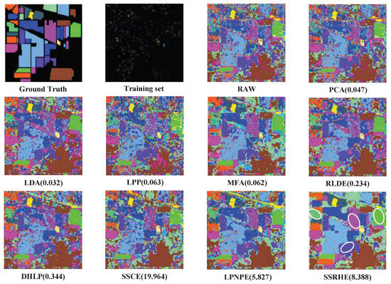
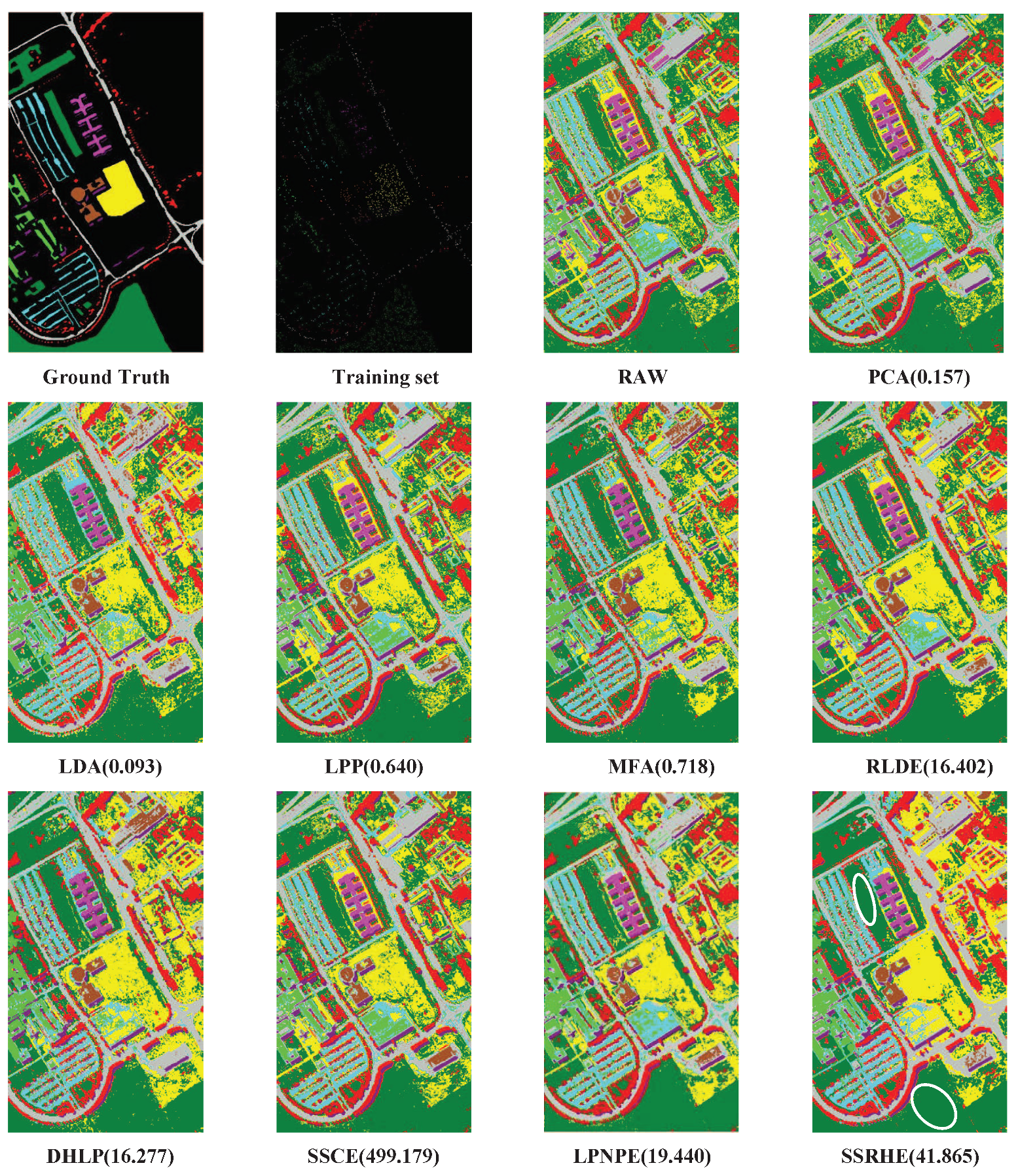
Figure 10. Classification maps of different DR methods with 1-NN on the Indian Pines dataset. Note that the time cost of corresponding DR algorithms is marked in bracket.

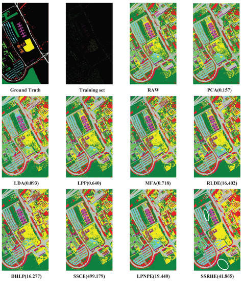
Figure 11. Classification maps of different DR methods with 1-NN on the PaviaU dataset. Note that the time cost of corresponding DR algorithms is marked in bracket.

According to Table 3 and Table 4, SSRHE obtained better classification results than other methods in most classes, and it achieved the best OA, AA and KC on two HSI datasets. This indicates that SSRHE possessed stronger ability to reveal the intrinsic complex geometric relations between samples and extract more useful the spatial-spectral combined features for classification. As shown in Figure 10 and Figure 11, the spatial-spectral methods generally produced smoother classification maps than traditional spectral-based methods, which demonstrates that the spatial information in HSI is effective for improving classification performance. Moreover, the classification maps of SSRHE possessed fewer misclassified pixels, especially in the areas Grass/Pasture, Wheat, and Stone-steel towers for Indian Pines dataset and Asphalt, Meadows, and Shadows for PaviaU dataset. In terms of running time, SSRHE cost more time than traditional spectral-based methods because it needs to build models in both spatial domain and spectral domain of HSI data. Compared with other spectral-spatial algorithms, the running time of SSRHE did not increase significantly and was far less than SSCE. Thus, SSRHE was more effective than other DR methods to weaken the influence of noisy points and develop the discrimination power of embedding features.

5. Conclusions

In this paper, a new dimensionality reduction method SSRHE is proposed based on sparse hypergraph learning and spatial-spectral information for HSI. SSRHE computes two spatial neighborhood scatters to reveal the spatial correlation between each pixels in HSI, and it also constructs two discriminant hypergraphs by sparse representation to discover the complex multivariate relationships between interclass samples and intraclass samples, respectively. Based on the spatial neighborhood scatters and the Laplacian scatters of hypergraphs, a spatial-spectral combined objective function is designed to obtain an optimal projection matrix mapping original HSI data to low-dimensional embedding space where the intrinsic spatial and spectral properties are well preserved. some experiments were conducted on Indian Pines and PaviaU datasets to demonstrate that the proposed method possesses better performance compared with some existing state-of-the-art DR methods. In the future, we will optimize the proposed algorithm to reduce the running time and extend it to other related fields such as multi-spectral images and very-high resolution images, and the sparse hypergraph model in this paper can be used in some application domains with high-dimensional data such as face images, gene expression and radiomics features. Furthermore, It would also be interesting to study integrating hypergraph learning and heterogeneous information networks when exploring high-dimensional data with multiple adjacency relationships.

References

- Liao, D.; Qian, Y.; Tang, Y.Y. Constrained manifold learning for hyperspectral imagery visualization. IEEE J. Sel. Top. Appl. Earth Obs. Remote Sens. 2018, 1, 1213–1226. [Google Scholar] [CrossRef]
- Yuan, Q.Q.; Zhang, Q.; Li, J.; Li, J.; Zhang, L.P. Hyperspectral image denoising employing a spatial-spectral deep residual convolutional neural network. IEEE Trans. Geosci. Remote Sens. 2019, 57, 1205–1218. [Google Scholar] [CrossRef]
- Liu, Q.; Sun, Y.; Hang, R.; Song, H. Spatial-spectral locality-constrained low-rank representation with semi-supervised hypergraph learning for hyperspectral image classification. IEEE J. Sel. Top. Appl. Earth Obs. Remote Sens. 2017, 10, 4171–4182. [Google Scholar] [CrossRef]
- Zhang, X.R.; Gao, Z.Y.; Jiao, L.C.; Zhou, H.Y. Multifeature hyperspectral image classification with local and nonlocal spatial information via markov random field in semantic space. IEEE Trans. Geosci. Remote Sens. 2016, 56, 1409–1424. [Google Scholar] [CrossRef]
- Xu, Y.H.; Zhang, L.P.; Du, B.; Zhang, F. Spectral-spatial unified networks for hyperspectral image classification. IEEE Trans. Geosci. Remote Sens. 2018, 56, 5893–5909. [Google Scholar] [CrossRef]
- Kumar, B.; Dikshit, O. Spectral contextual classification of hyperspectral imagery with probabilistic relaxation labeling. IEEE Trans. Cybern. 2017, 47, 4380–4391. [Google Scholar] [CrossRef] [PubMed]
- Hang, R.; Liu, Q.; Sun, Y.; Yuan, X.; Pei, H.; Plaza, J.; Plaza, A. Robust matrix discriminative analysis for feature extraction from hyperspectral images. IEEE J. Sel. Top. Appl. Earth Obs. Remote Sens. 2017, 10, 2002–2011. [Google Scholar] [CrossRef]
- Luo, F.L.; Huang, H.; Ma, Z.Z.; Liu, J.M. Semi-supervised sparse manifold discriminative analysis for feature extraction of hyperspectral images. IEEE Trans. Geosci. Remote Sens. 2016, 54, 6197–6221. [Google Scholar] [CrossRef]
- Xu, J.; Yang, G.; Yin, Y.F.; Man, H.; He, H.B. Sparse representation based classification with structure preserving dimension reduction. Cogn. Comput. 2014, 6, 608–621. [Google Scholar] [CrossRef]
- Zabalza, J.; Ren, J.C.; Yang, M.Q.; Zhang, Y.; Wang, J.; Marshall, S.; Han, J.W. Novel folded-PCA for improved feature extraction and data reduction with hyperspectral imaging and SAR in remote sensing. ISPRS J. Photogramm. Remote Sens. 2014, 93, 112–122. [Google Scholar] [CrossRef]
- Li, W.; Prasad, S.; Fowler, J.E. Noise-adjusted subspace discriminant analysis for hyperspectral imagery classification. IEEE Geosci. Remote Sens. Lett. 2013, 10, 1374–1378. [Google Scholar] [CrossRef]
- Roweis, S.T.; Saul, L.K. Nonlinear dimensionality reduction by locally linear embedding. Science 2000, 290, 2323–2326. [Google Scholar] [CrossRef]
- Chen, C.; Zhang, L.; Bu, J.; Wang, C.; Chen, W. Constrained laplacian eigenmap for dimensionality reduction. Neurocomputing 2010, 73, 951–958. [Google Scholar] [CrossRef]
- Bachmann, C.M.; Ainsworth, T.L.; Fusina, R.A. Exploiting manifold geometry in hyperspectral imagery. IEEE Trans. Geosci. Remote Sens. 2005, 43, 441–454. [Google Scholar] [CrossRef]
- He, X.F.; Cai, D.; Yan, S.C.; Zhang, H.J. Neighborhood preserving embedding. In Proceedings of the Tenth IEEE International Conference on Computer Vision (ICCV’05), Beijing, China, 17–21 October 2005; Volume 2, pp. 1208–1213. [Google Scholar]
- Zheng, Z.L.; Yang, F.; Tan, W.; Jia, J.; Yang, J. Gabor feature-based face recognition using supervised locality preserving projection. Signal Process. 2007, 87, 2473–2483. [Google Scholar] [CrossRef]
- Huang, H.; Yang, M. Dimensionality reduction of hyperspectral images with sparse discriminant embedding. IEEE Trans. Geosci. Remote Sens. 2015, 53, 5160–5169. [Google Scholar] [CrossRef]
- Jiang, X.; Song, X.; Zhang, Y.; Jiang, J.; Gao, J.; Cai, Z. Laplacian regularized spatial-aware collaborative graph for discriminant analysis of hyperspectral imagery. Remote Sens. 2019, 11, 29. [Google Scholar] [CrossRef]
- Hang, R.; Liu, Q. Dimensionality reduction of hyperspectral image using spatial regularized local graph discriminant embedding. IEEE J. Sel. Top. Appl. Earth Obs. Remote Sens. 2018, 11, 3262–3271. [Google Scholar] [CrossRef]
- Feng, F.B.; Li, W.; Du, Q.; Zhang, B. Dimensionality reduction of hyperspectral image with graph-based discriminant analysis considering spectral similarity. Remote Sens. 2017, 9, 323. [Google Scholar] [CrossRef]
- Luo, F.L.; Huang, H.; Duan, Y.L.; Liu, J.M.; Liao, Y.H. Local geometric structure feature for dimensionality reduction of hyperspectral imagery. Remote Sens. 2017, 9, 790. [Google Scholar] [CrossRef]
- Sugiyama, M. Dimensionality reduction of multimodal labeled data by local fisher discriminant analysis. J. Mach. Learn. Res. 2007, 8, 1027–1061. [Google Scholar]
- Zhou, Y.C.; Peng, J.T.; Philip Chen, L.C. Dimension reduction using spatial and spectral regularized local discriminant embedding for hyperspectral image classification. IEEE Trans. Geosic. Remote Sens. 2015, 53, 1082–1095. [Google Scholar] [CrossRef]
- Huang, Y.; Liu, Q.; Zhang, S.; Metaxas, D. Image retrieval via probabilistic hypergraph ranking. In Proceedings of the 2010 IEEE Computer Society Conference on Computer Vision and Pattern Recognition, San Francisco, CA, USA, 13–18 June 2010; pp. 3367–3383. [Google Scholar]
- Liu, Q.; Sun, Y.; Wang, C.; Liu, T.; Tao, D. Elastic net hypergraph learning for image clustering and semi-supervised classification. IEEE Trans. Image Process. 2017, 26, 452–463. [Google Scholar] [CrossRef] [PubMed]
- Yu, J.; Tao, D.; Wang, M. Adaptive hypergraph learning and its application in image classification. IEEE Trans. Image Process. 2012, 21, 3262–3272. [Google Scholar]
- Wang, W.H.; Qian, Y.T.; Tang, Y.Y. Hypergraph-regularized sparse NMF for hyperspectral unmixing. IEEE J. Sel. Top. Appl. Earth Obs. Remote Sens. 2016, 9, 681–694. [Google Scholar] [CrossRef]
- Huang, S.; Yang, D.; Ge, Y.X.; Zhang, X.H. Discriminant hyper-Laplacian projection and its scalable extension for dimensionality reduction. Neurocomputing 2016, 173, 145–153. [Google Scholar] [CrossRef]
- Du, W.B.; Qiang, W.W.; Lv, M.; Hou, Q.L.; Zhen, L.; Jing, L. Semi-supervised dimension reduction based on hypergraph embedding for hyperspectral images. Int. J. Remote Sens. 2018, 39, 1696–1712. [Google Scholar] [CrossRef]
- Gao, S.H.; Tsang, I.W.H.; Chia, L.T. Laplacian sparse coding, hypergraph Laplacian sparse coding, and applications. IEEE Trans. Pattern Anal. Mach. Intell. 2013, 35, 92–104. [Google Scholar] [CrossRef] [PubMed]
- Pio, G.; Serafino, F.; Malerba, D.; Ceci, M. Multi-type clustering and classification from heterogeneous networks. Inf. Sci. 2018, 425, 107–126. [Google Scholar] [CrossRef]
- Serafino, F.; Pio, G.; Ceci, M. Ensemble learning for multi-type classification in heterogeneous networks. IEEE Trans. Knowl. Data Eng. 2018, 30, 2326–2339. [Google Scholar] [CrossRef]
- Liao, W.Z.; Mura, M.D.; Chanussot, J.; Pizurica, A. Fusion of spectral and spatial information for classification of hyperspectral remote sensed imagery by local graph. IEEE J. Sel. Top. Appl. Earth Obs. Remote Sens. 2018, 9, 583–594. [Google Scholar] [CrossRef]
- Zhao, J.; Zhong, Y.F.; Shu, H.; Zhang, L.P. High-resolution image classification integrating spectral-spatial-location cues by conditional random fields. IEEE Trans. Image Process. 2016, 25, 4033–4045. [Google Scholar] [CrossRef]
- Cao, J.; Wang, B. Embedding learning on spectral-spatial graph for semi-supervised hyperspectral image classification. IEEE Geosci. Remote Sens. Lett. 2017, 14, 1805–1809. [Google Scholar] [CrossRef]
- Zhao, W.; Du, S. Spectral-spatial feature extraction for hyperspectral image classification: A dimension reduction and deep learning approach. IEEE Trans. Geosci. Remote Sens. 2016, 54, 4544–4554. [Google Scholar] [CrossRef]
- Li, Y.; Zhang, H.; Shen, Q. Spectral-spatial classification of hyperspectral imagery with 3D convolutional neural network. Remote Sens. 2017, 9, 67. [Google Scholar] [CrossRef]
- Wu, Z.B.; Shi, L.L.; Li, J.; Wang, Q.C.; Sun, L.; Wei, Z.H.; Plaza, J.; Plaza, A.J. GPU parallel implementation of spatially adaptive hyperspectral image classification. IEEE J. Sel. Top. Appl. Earth Obs. Remote Sens. 2018, 11, 1131–1143. [Google Scholar] [CrossRef]
- Mohan, A.; Sapion, G.; Bosch, E. Spatially coherent nonlinear dimensionality reduction and segmentation of hyperspectral images. IEEE Geosci. Remote Sens. Lett. 2007, 4, 206–210. [Google Scholar] [CrossRef]
- Huang, H.; Zheng, X.L. Hyperspectral image land cover classification algorithm based on spatial-spectral coordination embedding. Acta Geod. Cartogr. Sin. 2016, 4, 964–972. [Google Scholar]
- Feng, Z.X.; Yang, S.Y.; Wang, S.G.; Jiao, L.C. Discriminative spectral-spatial margin-based semisupervised dimensionality reduction of hyperspectral data. IEEE Geosci. Remote Sens. Lett. 2015, 12, 224–228. [Google Scholar] [CrossRef]
- Ji, R.R.; Gao, Y.; Hong, R.C.; Liu, Q.; Tao, D.C.; Li, X.L. Spectral-spatial constraint hyperspectral image classification. IEEE Trans. Geosci. Remote Sens. 2014, 52, 1811–1824. [Google Scholar]
- Luo, F.L.; Du, B.; Zhang, L.P.; Zhang, L.F.; Tao, D.C. Feature learning using spatial-spectral hypergraph discriminant analysis for hyperspectral image. IEEE Trans. Cybern. 2019, 49, 2406–2419. [Google Scholar] [CrossRef]
- Tang, Y.Y.; Lu, Y.; Yuan, H. Hyperspectral image classification based on three-dimensional scattering wavelet transform. IEEE Trans. Geosci. Remote Sens. 2015, 53, 2467–2480. [Google Scholar] [CrossRef]
- Sun, Y.B.; Wang, S.J.; Liu, Q.S.; Hang, R.L.; Liu, G.C. Hypergraph embedding for spatial-spectral joint feature extraction in hyperspectral images. Remote Sens. 2017, 9, 506. [Google Scholar]
- Yuan, H.L.; Tang, Y.Y. Learning with hypergraph for hyperspectral image feature extraction. IEEE Geosci. Remote Sens. Lett. 2015, 12, 1695–1699. [Google Scholar] [CrossRef]
- Sun, Y.; Hang, R.; Liu, Q.; Zhu, F.; Pei, H. Graph-rRegularized low rank representation for aerosol optical depth retrieval. Int. J. Remote Sens. 2016, 37, 5749–5762. [Google Scholar] [CrossRef]
- Liu, J.; Xiao, Z.; Chen, Y.; Yang, J. Spatial-Spectral graph regularized kernel sparse representation for hyperspectral image classification. ISPRS Int. J. Geo-Inf. 2017, 6, 258. [Google Scholar] [CrossRef]
- Zhang, S.Q.; Li, J.; Li, H.C.; Deng, C.Z.; Antonio, P. Spectral-spatial weighted sparse regression for hyperspectral image unmixing. IEEE Trans. Geosci. Remote Sens. 2018, 56, 3265–3276. [Google Scholar] [CrossRef]
- Sun, W.W.; Zhang, L.F.; Zhang, L.P.; Yenming, M.L. A dissimilarity-weighted sparse self-representation method for band selection in hyperspectral imagery classification. IEEE J. Sel. Top. Appl. Earth Observ. Remote Sens. 2016, 9, 4374–4388. [Google Scholar] [CrossRef]
- Luo, M.N.; Zhang, L.L.; Liu, J.; Zheng, Q.H. Distributed extreme learning machine with alternating direction method of multiplier. Neurocomputing 2017, 261, 164–170. [Google Scholar] [CrossRef]
© 2019 by the authors. Licensee MDPI, Basel, Switzerland. This article is an open access article distributed under the terms and conditions of the Creative Commons Attribution (CC BY) license (http://creativecommons.org/licenses/by/4.0/).