ImaACor: A Physically Based Tool for Combined Atmospheric and Topographic Corrections of Remote Sensing Images

Abstract

ImaACor is a tool for the simultaneous correction of remotely sensed data from atmospheric and topographic effects, including second-order corrections, such as adjacency effects. The implemented approach is physically based and uses MODTRAN for computation of the main radiometric quantities. A user-friendly, comprehensive, and exhaustive graphic interface allows the user to choose from different correction levels. The various panels allow one to set all the parameters to correctly characterize the atmosphere and define the acquisition and illumination geometries. The tool provides a number of facilities to easily manage the correction process for a wide range of sensor data, including the ability to process multiple data in batch mode, which is very useful for dealing with temporal series. Under the inclusion of topographic correction, this tool allows the user to select a digital elevation model that is automatically resampled to the image resolution and processed to obtain the parameters for radiometric transfer modeling and the subsequent harmonization of the surface with the model inversion. This tool also includes utilities for the pre-processing of PRISMA data.

1. Introduction

The increased performance of satellite sensors requires a high-quality pre-processing chain to support remote sensing analysis in many fields [1]. In this context, atmospheric correction is a critical step to maximize information content [2,3,4,5]. In contexts of terrain roughness, remotely sensed data must also be corrected for topographic effects because the irradiation on a slope strongly varies with the relative angle between the sun and the slope azimuth, thus impacting the remotely sensed signal [6,7,8]. This effect has to be properly modeled and corrected to enhance image quality. As sensor performance has increased, empirical approaches for atmospheric and topographic correction have been gradually replaced with physically based procedures.

In the literature, physically based models for atmospheric correction are often matched with empirical ones for topographic correction in the case of terrain roughness [9,10]. Although these studies have shown good results, a number of works have demonstrated the advantages of using a unique physically based model for the simultaneous correction of both atmospheric and topographic effects [11,12,13,14,15].

In this paper, the ImaACor (Image Atmospheric Correction) software is presented with an exhaustive and user-friendly GUI (graphic user interface); this tool’s facilities can easily manage the atmospheric correction process. This software allows one to atmospherically and topographically correct a wide range of remote sensing data and implements a fully physically based approach based on MODTRAN 4 simulations. The software, under the assumption of a Lambertian surface, can also implement a model for the simulation and correction of the impact of the environment on a remotely sensed signal. The models implemented in the tool were tested in various contexts and showed great potential for improving remotely sensed products, as shown in [4]. Many facilities to manage multiple or redundant applications are provided to reuse the calculated quantities and speed up the processing activities. After the launch of the PRISMA mission, the software was equipped with a set of features for the pre-processing and re-calibration of PRISMA data.

2. Models

2.1. Atmospheric Model

This software implements different models with different complexity levels. When both adjacency and topographic correction are selected, the model is represented by the following equation from [4]:

$$L=A_d\rho \cdot \frac{cos(i)}{cos({\theta }_s)}+\left[A\frac{\rho }{\left(1-S{\rho }_e\right)}-A_d\rho \right]\cdot \frac{\left(\pi -\alpha \right)}{\pi }+B\frac{{\rho }_e}{\left(1-S{\rho }_e\right)}+L_{path},$$

(1)

where L is the sensor radiance; L_path is the path radiance (the solar signal reflected by the atmosphere and not reaching the surface); $\rho$ is the target reflectance; ${\rho }_e$ is the background reflectance; S is the spherical albedo; and A, A_d, and B are parameters that do not depend on the surface properties and can be expressed as a function of the downward and upward (diffuse and direct) transmittances, of the solar zenith angle and solar flux at the top of the atmosphere. In particular, A does not depend on upward diffuse transmittance, B does not depend on direct upward transmittance, and A_d only depends on direct transmittance [4]. The first term of the second member represents the contribution of the target due to the direct light that is directly reflected onto the sensor. The impact of the sloped terrain on this term is modelled by considering the angle $i$, defined as the angle between the incoming solar radiation and the normal to the surface that, for an inclined surface, is different from the sun zenith angle ${\theta }_s$ [13]. For angles above π/2, $i$ is set to π/2. Under this condition, the target is in the shadow, and the term is zero. The second term accounts for the diffuse light that is directly reflected to the sensor. In this case, the scaling factor $\left(\pi -\alpha \right)/\pi$ considers the real portion of the sky dome viewed by the target, with $\alpha$ representing the slope angle between the inclined surface and the horizontal plane. The third term of the second member accounts for all the contributions diffused by the background. An exhaustive description of the model that includes all the steps to derive it can be found in Santini and Palombo (2019).

When the topographic correction is not selected, $cos(i)=cos({\theta }_s)$ and $\alpha =0$. In this condition, the terms including A_d, compensate for each other, and a simpler model can be considered:

$$L=A\frac{\rho }{\left(1-S{\rho }_e\right)}+B\frac{{\rho }_e}{\left(1-S{\rho }_e\right)}+L_{path}.$$

(2)

If the correction of the adjacency effect is not selected, ${\rho }_e=\rho$. When no topographic and adjacency effects are selected, the model regresses to the simplified and most well-known model:

$$L=A^{\prime }\frac{\rho }{\left(1-S\rho \right)}+L_{path},$$

(3)

where $A^{\prime }=A+B$.

Different models are used when different combinations of correction options are selected.

2.2. MODTRAN Simulation

The physical quantities of the different models are simulated based on the MODTRAN 4 model. Although MODTRAN 4 works only with homogeneous surfaces, its output allows one to discriminate between the radiance reflected by the target and the radiance diffused by the background and also provides a separate output for reflectance contributions from only the direct incident light. Based on this output, ImaACor keeps all the terms of the second member of Equation (1) separate.

MODTRAN allows one to manage many parameters to simulate the necessary radiative quantities, based on the sensor and platform characteristics, the illumination and acquisition geometry, the surface elevation, and the atmospheric conditions and characteristics. MODTRAN can also simulate the quantities in a wide range of frequencies with a resolution as low as one cm⁻¹ and provides several options for atmospheric scattering simulation, including multiple scattering models [16]. Depending on the correction selected, ImaACor operates a different set of MODTRAN simulations to estimate all the physical quantities of the Equations (1)–(3) ($L_{path}$, $A$, $B$, $A_d$, $S$, and other quantities needed for the estimation of the environmental contribution). The ImaACor GUI allows the user to manage all the MODTRAN input parameters needed to properly model the atmosphere and gives the user a choice between different operation modalities, as described in the section dedicated to the GUI.

2.3. Environmental Function

When the adjacency effect correction is selected, the $\rho$ is first estimated based on the simplified model of Equation (3). Then, ${\rho }_e$ is computed on the basis of an environmental function $F\left(r\right)$, which describes the efficiency of the atmospheric transmission of the signal reflected by a point located at a distance $r$ from the target. In polar coordinates, for a nearly nadir view, this relation between ${\rho }_e$ and $F\left(r\right)$ can be expressed by the following equation from [17]:

$${\rho }_e=\frac{1}{2\pi }{{\displaystyle \int }}_0^{2\pi }{{\displaystyle \int }}_0^{+\infty }\rho \left(\phi ,r\right)\frac{dF\left(r\right)}{dr}drd\phi .$$

(4)

The environment function accounts for the probability that a photon within a distance $r$ from the target will be scattered to the sensor. Its derivative, $\frac{dF\left(r\right)}{dr}$, is known as the atmospheric point spread function. The $F\left(r\right)$ depends on many parameters, including the phase functions of the molecules and aerosols, their vertical distribution, and their optical thickness [7,16,17,18,19,20]. The derivation of the function $F\left(r\right)$ is completely described in [4].

After obtaining ${\rho }_e$, Equation (1) is used to derive the final reflectance $\rho$. ImaACor offers different options for estimating $F\left(r\right)$ and ${\rho }_e$, with different precisions and processing times. The most accurate modality allows the construction and rigorous application of the environmental function described in [17]. This modality is highly time consuming and should be used only after all other atmospheric parameters have been defined to avoid unnecessary time expenditures. Once computed, ${\rho }_e$ can be stored for further applications. A much less time-consuming modality, but with a performance very similar to that of rigorous applications, can be obtained by applying a series of low pass filters to simulate the effect of the environmental function at various distances from the target.

2.4. Digital Elevation Model

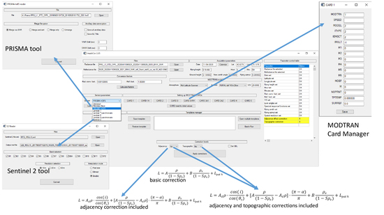
When topographic correction is selected, the $i$ and $\alpha$ angles of Equation (1) and the shaded areas are automatically computed by the tool on the basis of the DEM (digital elevation model) that is loaded by the user through the graphic interface. The computed parameters can then be saved in a single file (named associated DEM) and reloaded in subsequent applications to reduce the processing time. The DEM is also used as the input in MODTRAN simulations to account for height variations in the atmospheric column.

3. ImaACor GUI

ImaACor is provided with a user-friendly and exhaustive GUI, which allows the complete management of all data and implemented features. This GUI is organized with a main panel (Figure 1) divided into sections for different functionalities. Each section allows the user to insert or select data and operate his or her choices through a series of dedicated menus and panels. This section is dedicated to a description of the GUI and its ability to manage the main features implemented in ImaACor. The following list briefly describes all the sections of the main panel:

• “File”: manages the input and output of files.
• “Acquisition parameters”: manages the image acquisition parameters.
• “Conversion factors”: allows the setting of conversion factors.
• “MODTRAN Models”: manages the setting of atmospheric models for MODTRAN simulations.
• “Sensor parameters”: manages the setting of the instrumental parameters.
• “Setting up MODTRAN cards”: manages the MODTRAN card parameters.
• “DEM Processing”: manages the processing of the DEM for topographic correction.
• “R_rs processing”: allows the computation of remote sensing reflectance for water bodies.
• “Template manager”: manages templates (also for multiple runs in batch mode).
• “Correction levels”: allows one to set the corrections to be performed and start the correction process.
• “Parameter control table”: shows the set parameters.

3.1. File

The “file” section allows the user to open the radiance file to be processed and select the reflectance file to save the result of the atmospheric correction. This tool provides a utility to automate the choice of the output file name through a series of suffixes corresponding to the different parameters considered during correction. This is particularly useful for multiple processing (see the dedicated section). Moreover, the automation of the naming process drastically reduces the risk of unintentionally overwriting the files and allows the user to always immediately obtain correct information about the content of a file starting from its name. The user is allowed to select the various suffixes to be used in the automated naming process through a choice menu (Figure 2). The first suffix added to the base name is “_refl” (reflectance) and is mandatory. The other selectable suffixes relate to the correction levels applied to the image and to the values of the atmospheric and image acquisition parameters used for the correction: (i) “_adj” refers to the correction of the adjacency effect; (ii) “_topo” refers to the topographic correction; (iii) “_rrs” refers to the remote sensing reflectance (used for the water’s surface); (iv) “_vis_xxx” refers to the values of the visibility; (v) “_H2O_xxx” refers to the atmospheric column water content, etc. The choice menu with the complete set of suffixes to be selected appears when the F12 key is pressed.

3.2. Acquisition Parameters

The “acquisition parameters” section allows the setting of the geographic coordinates, the date and time, and the other acquisition parameters. The settable parameters are:

• Date (dd/mm/yyyy).
• Latitude (decimal format).
• Longitude (decimal format).
• Flying height (km).
• Hour (hh).
• Minutes (mm).
• Ground height (km).
• Flying zenith (degree).
• Flying azimuth (degree).

The acquisition date can also be set using a date picker that appears when the calendar” button is pressed. If geographic information is present in the header associated with the image, the latitude and longitude values of the image center are automatically loaded and shown in their proper fields. Starting from the image latitude and longitude, the height is automatically computed using world DEM data stored in the “world_dem_geo_jpg.jp2” file.

3.3. Conversion Factors

This section allows one to set the scale factor to convert the radiance image into a MODTRAN radiance unit (µW/(cm²*nm*sr)). This form also allows one to set the conversion factor for output reflectance images. If the reflectance factor is set to 1, the output image will be a floating point; otherwise, it will be an unsigned integer with the reflectance value multiplied by the set reflectance factor. The “calculate factor” button calculates the radiance conversion factor starting from the input image radiance units, which must be set in the left column of the drop list menu (Figure 3).

3.4. MODTRAN Models

The “MODTRAN models” section allows the user to select the aerosol model and one of the six geographical-seasonal atmospheric MODTRAN models using the “atmosphere drop list menu”. The VIS form allows one to set the visibility.

3.5. Sensor Parameters

The “sensor parameters” section allows the user to set the spectral responses and to define the look angles associated with each across track pixel. This section also includes a drop-down menu for the selection of a known sensor for specific configurations or data pre-elaboration.

When clicked, the “look angles” button opens a panel (Figure 4) to configure the look angles in two modalities: (i) Opening a file containing the look angles for each pixel of the scan line, and (ii) setting the FOV (field of view) and the number of across track pixels to allow the system to compute the look angles. The computed look angle configuration is stored in the file selected by the user. If the “do not use look angles” box is flagged, the system associates the view angle corresponding to the inclination of the sensor axis during the acquisition (“vew zenith” value set on the principal panel) with each image pixel.

The “responses” button opens a panel to define the spectral response functions (Figure 5). The user can choose to open a file containing the spectral response functions in the ENVI (environment for visualizing images) spectral library format (“load from file”) or to open a file containing two columns with the wavelength of the band centers and related FWHM (full width at half maximum). In the latter case, the spectral response function of each band is built as a Gaussian function centered at the band center and with a standard deviation of $\mathsf{\sigma }=\frac{FWHM}{\sqrt{2ln2}}$. After selection, the spectral response functions of all bands are stored in the ENVI spectral format and plotted in the appropriate display (Figure 5).

The drop-down menu (Figure 6) allows the selection of a specific sensor within a list. When a sensor is selected, the system automatically loads or computes the appropriate spectral responses and asks the user to select a file (generally provided with the image data) with the acquisition parameters to be loaded (i.e., MTL.txt for Landsat 7/8 multispectral or panchromatic images and .xml for Sentinel 2 images). The loaded parameter values are shown in the appropriate fields of the main interface panel (Figure 1).

Within the selectable sensors, there are two modes referring to PRISMA: “PRISMA_ENVI”, and “PRISMA_HDF5”. When “PRISMA_ENVI” is selected, the user is asked to select a PRISMA image in the ENVI format and is allowed to select the original .he5 file to automatically load the acquisition parameters. The “PRISMA_HDF5” option allows one to directly use the PRISMA proprietary format .he5 through a dedicated interface, the “PRIMA reader tool” (Figure 7).

The PRISMA reader tool allows the user to convert the images from the .hdf5 to ENVI format. There are four options to convert the data: (i) “Merge via SNR”, which merges the VNIR and SWIR images by selecting the overlapping bands on the basis of the highest nominal SNR value; (ii) “merge and sort”, which merges the VNIR and SWIR images without operating any selection but sorting all the bands by wavelength order; (iii) “merge only”, which creates a merged image with the VNIR bands preceding the SWIR bands; and (iv) unmerge, which saves the VNIR and SWIR images in two separate files in the ENVI format. The ENVI header file is built to include a series of ancillary information, such as wavelength and FWHM. By pressing the “save all ancillary data” button of the PRISMA reader tool, all ancillary data contained in the .he5 file are stored in separate files in ENVI format with the same name used in the original .he5 file. Finally, the tool also allows the user to operate spectral shift for the VNIR and SWIR separately to correct for a possible shift of the original data.

3.6. Settings up the MODTRAN Cards

In this section of the main graphic display, it is possible to manage all the MODTRAN cards to be used for the atmospheric simulations. Each button of the interface opens an interface for a specific card. In Figure 8, an example of a MODTRAN card setting interface is shown. By pressing the “cards reset to initial values” button (Figure 1), all MODTRAN cards are reset to the values stored in the “card.ini” file, which is updated each time the main graphic display is closed.

3.7. DEM Processing

In the “DEM processing” section, the “associate DEM” button opens the “associate image–DEM” interface (Figure 9). This interface allows one to select a DEM (georeferenced DEM), which is used to compute the other parameters needed for operating the topographic correction. The result is a multilayer image, referred to as an ‘associated DEM’, made up of five layers. The first layer constitutes the actual elevation model, while the other layers consist of the derived parameters: (ii) sun angle; (iii) shadow; (iv) slope; and (v) image mask. The ‘associated DEM’ is stored in a file named radiance file name + _dem and can be reloaded for further processing through the “choose associated DEM” button.

The “associate image–DEM” interface offers three options to manage the shadow correction: (i) “Calculate the shadow”, which uses ImaACor to calculate the shaded areas based on the uploaded DEM; (ii) “open the shadow file”, which allows the selection of a file containing a mask of the shaded areas; and (iii) “skip the shading correction”, which skips the shadow correction.

3.8. R_rs Processing

The “R_rs processing” section allows one to calculate the remote sensing reflectance, which is the quantity usually used for water surfaces. This quantity excludes the contribution of the light reflected by the water surface and considers only the signal from the water column [4]. The software, in beta version, currently implements only an empirical estimate of the R_rs. This estimate is carried out by subtracting, from a reflectance image, the average value recorded in a certain range in the infrared region, where the R_rs is expected to be almost zero.

The “R_rs estimate” button gives access to the interface to estimate the R_rs value (Figure 10). This interface allows one to load and display (“load RGB”) a reflectance image. Using the left mouse button on the displayed image, it is possible to draw a ROI (region of interest) on a water area. At this point, the spectra of the ROI are plotted on the display, and the user is allowed to select the SWIR interval for the R_rs estimate using the mouse buttons. The converted R_rs image is then stored in the “R_rs output file” by pressing the “save” button.

3.9. Template Manager

The “template manager” allows one to save a complete set of run parameters in a template file; the “save template” and “restore template” buttons can be used to save and restore the template information. It is also possible to open several templates simultaneously to be processed in batch mode, which is useful both in the case of redundant applications on the same image and when a temporal series of images have to be processed.

ImaACor is also equipped with a template generator tool (Figure 11), which generates a series of templates that vary some parameters in a given interval. The tool opens when the F11 key is pressed. Template generation is initialized by a base template that has to be opened by the user. Then, the user is allowed to define the intervals and the steps of the parameters he or she wants to vary. The tool then generates a template for each combination of the set parameters, allowing the user to concurrently test a wide spectrum of correction parameters in batch mode.

3.10. Correction Levels

This section allows one to select the correction to be performed and starts the correction process. Any combination of adjacency and topographic correction can be selected, ranging from a base correction (if none of them are selected) to complete correction that includes both adjacency and topographic corrections and corresponds to the model in Equation (1).

When the adjacency correction is selected, an appropriate interface (Figure 12) allows the user to choose between two different modes for applying the environmental function (see Section 2.3), which differ in their rigor and processing time: (i) “Rigorously apply Equation (1)”, which is very expensive in terms of calculation time, and (ii) “perform a series of low-pass filters instead of computing the integral of the equation”, which significantly reduces the processing time with a small loss of precision. In both methods, the environment function is computed following [17], as explained in [4].

The interface also allows one to set the spatial resolution, which is automatically set when a geocoded radiance image is open. This value is used to compute the environmental function.

3.11. Control Table

In the parameter control table (Figure 13), the user can check the input of the correction parameters. Red refers to mandatory parameters, and yellow refers to optional parameters. Red and yellow are replaced by white after the parameters have been set.

4. ImaACor Application Results

This section illustrates some noteworthy results of the ImaACor application relating to topographic, adjacency, and shadow corrections.

Figure 14 presents a subset of a normalized spectral distance image [4] between two LANDSAT-8 images acquired from the arid region of Parinacota (Andes, Chile) in the same location but during different seasons (different illumination geometries) and corrected excluding (left) and including (right) topographic correction. The image shows remarkable flattening when topographic correction is included.

The two Parinacota images (centered at 19°20′0″S; 69°6′0″W) were acquired on 4/06/2016 (southern hemisphere winter) at 14:35 UTC and on 21/11/2016 (southern hemisphere summer) at 14:35 UTC.

To demonstrate adjacency correction, Figure 15 depicts a subset of a LANDSAT-8 image of Pertusillo Lake (Lucanian Apennines, Italy), a small inland water body surrounded by flourishing vegetation. In the same figure, the graph on the left shows the mean reflectance spectrum of the ROI on the lake (yellow rectangle), obtained while excluding (dashed line) and including (solid line) adjacency correction in the correction procedure. The graph clearly shows the presence of a sharp adjacency effect due to the near-infrared peak of vegetation on band 5, in which the water shows almost no signal due to water column absorption [5]. After the adjacency correction, the impact of the surrounding vegetation is greatly reduced. As the R_rs estimate was not included in the correction, a residual value in the infrared range is still present due to the water surface reflectance.

The Pertusillo image (centered at 40°10′0″N; 16°0′0″E and 40°17′0″N; 15°57′0″E) was acquired on 2019/08/24 at 9:35 UTC.

In Figure 16, an airborne CASI reflectance image acquired from an industrial area in the province of Reggio Calabria (Calabria, Italy) is shown before (Figure 16a) and after (Figure 16b) the application of topographic and shadow corrections. The results are remarkable, as the correction allowed almost complete recovery of the signal in the shade. This is confirmed by the graph in Figure 16c, which shows the spectra corresponding to an exposed and shaded portion of a paved road before and after shadow correction.

The Reggio Calabria image (centered at 37°56′57″N; 15°42′3″E) was acquired on 2013/01/08 at 8:30 UTC at 1240 m above sea level, corresponding to a spatial resolution of 0.50 m.

For a more detailed description of the above results, refer to [4].

As a further demonstration of ImaACor’s potential, Figure 17 presents the results of applying adjacency correction on a soil target. Figure 17a depicts an agricultural area in the province of Metaponto (Basilicata, Italy). The graph of Figure 17b shows the reflectance signal at 871 nm, corresponding to very high vegetation reflectance values, along the transept (red arrow) drawn on Figure 17a before and after correction for adjacency effects. A 10% increase in the contrast index was obtained (calculated as (max − min)/(max + min)); as expected, the intensity increased in the vegetated areas but decreased in the bare soil. The correction was applied to a non-georeferenced image to avoid any kind of distortion that would have made the image less sharp, partially hiding the effects of the correction. For this reason, the abscissa of the graph shows the number of pixels from the beginning of the transept.

The Metaponto image (centered at 40°23′00″N; 16°50′28″E) was acquired on 2013/07/16 at 14:59:30 UTC at 3200 m above sea level, corresponding to a spatial resolution of about 1.50 m.

To determine the processing times, we carried out a series of typical runs on a standard 260-band PRISMA image on a PC equipped with an Intel(R) Core(TM) i7-7700HQ CPU @2.80 GHz. The results are shown in

Table 1. Typical processing times.

Adjacency	${\mathit{\rho }}_{\mathit{e}}\mathbf{Computation}$	Topographic	Processing Time
X	X	X	2:30 h
X	X	-	5:10 min
X	-	-	2:20 min
-	-	-	1:20 min

. The third row of the table refers to a case in which the correction of adjacency effects is included but a previously calculated ${\rho }_e$ image is reused.

5. Conclusions

This paper presents the ImaACor tool, including its various models and GUI. ImaACor is a versatile tool for the correction of remotely sensed data for atmospheric and topographic effects. The implemented models are physically based and take into account second-order corrections, such as adjacency effects. The software’s exhaustive and friendly GUI allows the user to manage the correction process, including MODTRAN simulations, to estimate the necessary atmospheric quantities. This tool includes several utilities for the pre-processing of PRISMA data and provides an instrument for the management of multiple data in batch mode, which is very practical when temporal series have to be pre-processed. The implemented methods demonstrate great potential, as shown in [4]. ImaACor is used on a daily basis to correct and enhance the quality of images in research contexts and experiences continuous updates. In the near future, the implementation of a physically based method for the derivation of the R_rs is planned.

6. Software Distribution

This software is currently distributed on demand. It is possible to request the beta version of ImaACor for evaluation purposes directly from the authors at [email protected] or [email protected]. The tool was implemented in a Windows environment and requires an IDL virtual machine 8 or higher and the installation of MODTRAN 4.

References

1. Guanter, L.; Del Carmen González-Sanpedro, M.; Moreno, J. A method for the atmospheric correction of ENVISAT/MERIS data over land targets. Int. J. Remote Sens. 2007, 28, 709–728. [Google Scholar] [CrossRef]
2. Acito, N.; Diani, M. Unsupervised Atmospheric Compensation of Airborne Hyperspectral Images in the VNIR Spectral Range. IEEE Trans. Geosci. Remote Sens. 2018, 56, 2083–2106. [Google Scholar] [CrossRef]
3. Amato, U.; Cavalli, R.; Palombo, A.; Pignatti, S.; Santini, F. Experimental Approach to the Selection of the Components in the Minimum Noise Fraction. IEEE Trans. Geosci. Remote Sens. 2008, 47, 153–160. [Google Scholar] [CrossRef]
4. Santini, F.; Palombo, A. Physically Based Approach for Combined Atmospheric and Topographic Corrections. Remote Sens. 2019, 11, 1218. [Google Scholar] [CrossRef] [Green Version]
5. Santini, F.; Alberotanza, L.; Cavalli, R.M.; Pignatti, S. A two-step optimization procedure for assessing water constituent concentrations by hyperspectral remote sensing techniques: An application to the highly turbid Venice lagoon waters. Remote Sens. Environ. 2010, 114, 887–898. [Google Scholar] [CrossRef]
6. Hantson, S.; Chuvieco, E. Evaluation of different topographic correction methods for Landsat imagery. Int. J. Appl. Earth Obs. Geoinf. 2011, 13, 691–700. [Google Scholar] [CrossRef]
7. Kawishwar, P. Atmospheric Correction Models for Retrievals of Calibrated Spectral Profiles from Hyperion EO-1 Data. Master’s Thesis, International Institute for Geo-Information Science and Earth Observation, Enschede, The Netherlands, 2007. [Google Scholar]
8. Shepherd, J.D.; Dymond, J. Correcting satellite imagery for the variance of reflectance and illumination with topography. Int. J. Remote Sens. 2003, 24, 3503–3514. [Google Scholar] [CrossRef]
9. Richter, R. Correction of atmospheric and topographic effects for high spatial resolution satellite imagery. Int. J. Remote Sens. 1997, 18, 1099–1111. [Google Scholar] [CrossRef]
10. Sandmeier, S.R.; Itten, K.I. A physically-based model to correct atmospheric and illumination effects in optical satellite data of rugged terrain. IEEE Trans. Geosci. Remote Sens. 1997, 35, 708–717. [Google Scholar] [CrossRef] [Green Version]
11. Guanter, L.; Kaufmann, H.; Segl, K.; Foerster, S.; Rogass, C.; Chabrillat, S.; Kuester, T.; Hollstein, A.; Rossner, G.; Chlebek, C.; et al. The EnMAP Spaceborne Imaging Spectroscopy Mission for Earth Observation. Remote Sens. 2015, 7, 8830–8857. [Google Scholar] [CrossRef] [Green Version]
12. Guanter, L.; Richter, R.; Kaufmann, H. On the application of the MODTRAN4 atmospheric radiative transfer code to optical remote sensing. Int. J. Remote Sens. 2009, 30, 1407–1424. [Google Scholar] [CrossRef]
13. Kobayashi, S.; Sanga-Ngoie, K. The integrated radiometric correction of optical remote sensing imageries. Int. J. Remote Sens. 2008, 29, 5957–5985. [Google Scholar] [CrossRef]
14. Richter, R.; Schläpfer, D. Geo-atmospheric processing of airborne imaging spectrometry data. Part 2: Atmospheric/topographic correction. Int. J. Remote Sens. 2002, 23, 2631–2649. [Google Scholar] [CrossRef]
15. Richter, R. Correction of satellite imagery over mountainous terrain. Appl. Opt. 1998, 37, 4004–4015. [Google Scholar] [CrossRef] [PubMed]
16. Berk, A.; Anderson, G.P.; Acharya, P.K.; Chetwynd, J.H.; Bernstein, L.S.; Shettle, E.P.; Matthew, M.W.; Adler-Golden, S.M. Modtran4 User’s Manual. 1 June 1999. Available online: ftp://ftp.pmodwrc.ch/pub/Vorlesung%20K+S/MOD4_user_guide.pdf (accessed on 17 April 2000).
17. Vermote, E.F.; Tanre, D.; Deuze, J.L.; Herman, M.; Morcette, J.-J. Second Simulation of the Satellite Signal in the Solar Spectrum, 6S: An overview. IEEE Trans. Geosci. Remote Sens. 1997, 35, 675–686. [Google Scholar] [CrossRef] [Green Version]
18. Reinersman, P.; Carder, K. Monte Carlo simulation of the atmospheric point-spread function with an application to correction for the adjacency effect. Appl. Opt. 1995, 34, 4453–4471. [Google Scholar] [CrossRef]
19. Sanders, L.C.; Schott, J.R.; Raqueno, R. A VNIR/SWIR atmospheric correction algorithm for hyperspectral imagery with adjacency effect. Remote Sens. Environ. 2001, 78, 252–263. [Google Scholar] [CrossRef]
20. Vermote, E.F.; Vermeulen, A. Atmospheric Correction Algorithm: Spectral Reflectances (MOD09), version 4.0; ATBD: Baltimore, MD, USA, 1999. [Google Scholar]
Figure 1. ImaACor main display.
Remotesensing 12 02076 g001
Figure 2. Choice menu for the selection of the suffixes.
Remotesensing 12 02076 g002
Figure 3. Drop menu for the radiance conversion factor computations.
Remotesensing 12 02076 g003
Figure 4. Look angle configuration interface.
Remotesensing 12 02076 g004
Figure 5. Spectral response function tool.
Remotesensing 12 02076 g005
Figure 6. Details of the principal panel, which highlights the “instrument” drop-down list menu.
Remotesensing 12 02076 g006
Figure 7. PRISMA hdf5 file reader and conversion tool.
Remotesensing 12 02076 g007
Figure 8. MODTRAN Card 1A.
Remotesensing 12 02076 g008
Figure 9. Associate DEM (digital elevation model) interface.
Remotesensing 12 02076 g009
Figure 10. Rrs estimation interface.
Remotesensing 12 02076 g010
Figure 11. Template generator tool.
Remotesensing 12 02076 g011
Figure 12. Adjacency correction modalities.
Remotesensing 12 02076 g012
Figure 13. Details of the principal panel showing the “parameter control table”.
Remotesensing 12 02076 g013
Figure 14. Normalized spectral distance images before (a) and after (b) the inclusion of topographic correction, operated via ImaACor software.
Remotesensing 12 02076 g014
Figure 15. Landsat-8 image of Pertusillo Lake (Lucanian Apennines, Italy); in the graph, the mean spectra of the central lake’s deep water before (dashed line) and after (solid line) the application of the comprehensive correction procedure are shown.
Remotesensing 12 02076 g015
Figure 16. CASI (compact airborne spectrographic imager) reflectance images before (a) and after (b) the application of shadow correction. The ROI (region of interest) of the zoomed area relates to the shadow (red) and exposed (blue) areas. The graph shows the mean spectra of the ROIs before and after the application of topographic corrections (c).
Remotesensing 12 02076 g016
Figure 17. (a) CASI reflectance image of a rural area in the area of Metaponto (Basilicata, Italy). (b) Reflectance signal at 871 nm along the transept (red arrow) before (dashed line) and after (solid line) the correction for adjacency effects.
Remotesensing 12 02076 g017