Small Object Detection in Remote Sensing Images Based on Super-Resolution with Auxiliary Generative Adversarial Networks

Abstract

This article tackles the problem of detecting small objects in satellite or aerial remote sensing images by relying on super-resolution to increase image spatial resolution, thus the size and details of objects to be detected. We show how to improve the super-resolution framework starting from the learning of a generative adversarial network (GAN) based on residual blocks and then its integration into a cycle model. Furthermore, by adding to the framework an auxiliary network tailored for object detection, we considerably improve the learning and the quality of our final super-resolution architecture, and more importantly increase the object detection performance. Besides the improvement dedicated to the network architecture, we also focus on the training of super-resolution on target objects, leading to an object-focused approach. Furthermore, the proposed strategies do not depend on the choice of a baseline super-resolution framework, hence could be adopted for current and future state-of-the-art models. Our experimental study on small vehicle detection in remote sensing data conducted on both aerial and satellite images (i.e., ISPRS Potsdam and xView datasets) confirms the effectiveness of the improved super-resolution methods to assist with the small object detection tasks.

1. Introduction

The detection of small objects in remote sensing images has been known to be a challenging problem in the domain due to the small number of pixels representing these objects within the image compared to the image size. For example, in very high resolution (VHR) Pleiades satellite images (50 cm/pixel), vehicles are contained within an area of about 40 pixels ($4\times 10$ pixels). To improve the detection of small objects, e.g., vehicles, ships, and animals in satellite images, conventional state-of-the-art object detectors in computer vision such as Faster R-CNN (Faster Region-based Convolutional Neural Network) [1], SSD (Single Shot Multibox Detector) [2], Feature Pyramid Network [3], Mask R-CNN [4], YOLOv3 (You Only Look Once version 3) [5], EfficientDet [6], or others—see a survey of 20-year object detection in [7]—can be specialized by reducing anchor sizes, using multi-scale feature learning with data augmentation to target these small object sizes. We mention here some recent proposed models to tackle generic small object detection such as the improved Faster R-CNN [8], Feature-fused SSD [9], RefineDet [10], SCAN (Semantic context aware network) [11], etc. For more details about their architectures and other developed models, we refer readers to a recent review on deep learning-based small object detection in the computer vision domain [12]. Back to the remote sensing domain, some efforts have been made to tackle the small object detection task by adapting the existing detectors. In [13], Deconvolutional R-CNN was proposed by setting a deconvolutional layer after the last convolutional layer in order to recover more details and better localize the position of small targets. This simple but efficient technique helped to increase the performance of ship and plane detection compared to the original Faster R-CNN. In [14], an IoU-adaptive deformable R-CNN was developed with the goal of adapting IoU threshold according to the object size, to make dealing with small objects whose loss, according to the authors, would be absorbed during training phase easier. In [15], UAV-YOLO was proposed to adapt the YOLOv3 to detect small objects from unmanned aerial vehicle (UAV) data. Slight modification from YOLOv3 was done by concatenating two residual blocks of the network backbone having the same size. By focusing more on the training optimization of their dataset with UAV-viewed perspectives, the authors reported superior performance of UAV-YOLO compared to YOLOv3 and SSD. Another enhancement of YOLOv3 was done in [16] where the proposed YOLO-fine is able to better deal with small and very small objects thanks to its finer detection grids. In [17], the authors exploited and adapted the YOLOv3 detector for the detection of vehicles in Pleiades images at 50 cm/pixel. For this purpose, a dataset of 88 k vehicles was manually annotated to train the network. This approach, therefore, has the drawback of costly manual annotation and, in the case of application to images from another satellite sensor, a new annotation phase would be necessary. Moreover, by further reducing the resolution of these images (1 m/pixel), we may reach the limits of the detection capacity of those detectors (shown later through our experimental study).

An alternative approach that draws attention of researchers is to perform super-resolution (SR) to increase the spatial resolution of the images (and thus the size and details of the objects) before performing the detection task. To deal with the lack of details in the low-resolution images, the latest neural network super-resolution (SR) techniques such as Single Image Super-resolution (SI-SR) [18], CNN-based SR (SR-CNN) [19,20], Very Deep Super-resolution (VDSR) [21], Multiscale Deep Super-resolution (MDSR), Enhanced Deep Residual Super-resolution (EDSR) [22], Very Deep Residual Channel Attention Networks (RCAN) [23], Second-order Attention Network SR (SAN) [24], Super-Resolution with Cascading Residual Network (CARN) [25], etc. aim at significantly increasing the resolution of an image much better than the classical and simple bicubic interpolation. For example, while a VDSR model [21] uses a great number of convolutional layers (very deep), an EDSR network [22] stacks residual blocks to generate super-resolved images with increased spatial resolution from low-resolution (LR) ones. Readers interested in these networks are invited to read the recent review articles on deep learning-based super-resolution approaches in [26,27]. Back to the exploration of SR techniques to assist the detection task in the literature, some recent studies on detecting small objects thus exploit the above SR methods to increase image resolution so that the detector can search for larger objects (i.e., in super-resolved images). In [28], the authors combined an SR network which is upstream of the SSD detector for vehicle detection on satellite images, with only slight modifications to the first SSD layers. They have shown that an SSD working on super-resolved images (by a factor of 2 and 4) could yield significant improvement compared to the use of LR images. In addition, the authors in [29] described the gain provided by super-resolution with EDSR for different resolutions in satellite images. They observed that these techniques could considerably improve the SR results for 30-cm images with a factor of 2 (allowing to reach a spatial resolution of 15 cm), but not with a higher factor (of 4, 6, or 8 for example). 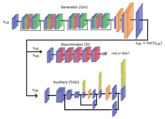In [30], the authors proposed an architecture with three components: an enhanced super-resolution with residual-based generative adversarial network (GAN), an edge enhancement network, and a detector network (Faster R-CNN or SSD). They performed an end-to-end training in which the gradient of the detection loss of the detector is back-propagated into the generator of the GAN network. They have provided significant improvement in detection of cars and gas storage within VHR images at 15-cm and 30-cm resolution with an SR factor of 4.

Indeed, the higher the super-resolution factor required (even lower resolution), the greater the number of residual blocks and the sizes of these blocks (size of the convolution layers) must be in order to reconstruct the image correctly. A simple network with an evaluation or optimization criterion such as MAE (Mean Absolute Error) or MSE (Mean Square Error) is thus particularly difficult to train due to the large number of parameters. In this article, our motivation is to develop novel solutions to improve a super-resolution framework with a final goal of detecting small objects in remote sensing images. We start in Section 2 with a brief introduction of the EDSR architecture for super-resolution that we select as our baseline model to develop different improvement strategies, without loss of generality. We then present in Section 3 the proposed improvements based on EDSR, respectively by integrating the Wasserstein generative adversarial network within a cycle model and adding an auxiliary network specified for object detection. To confirm and validate the effectiveness of our proposed strategies, we conduct an experimental study in Section 4 to evaluate detection performance of small objects in aerial imagery using the ISPRS data [31]. More precisely, we seek to extract vehicles on images whose spatial resolution has been artificially reduced to 1 m/pixel (by a factor of 8 from original 12.5-cm/pixel images). The objects we are looking for thus cover an area of approximately 10 pixels (for example $2\times 5$ pixels for a car). We report several qualitative and quantitative results of super-resolution and object detection that experimentally illustrate the interest of our strategies (Section 4.1). The generalization capacity of the proposed strategies is also studied by investigating another baseline SR network as well as several object detection models (Section 4.2 and Section 4.3). Then, we investigate the advantage of the proposed techniques within a multi-resolution transfer learning context where experiments are conducted on satellite xView data at 30-cm resolution [32] (Section 4.4). Finally, Section 5 draws some conclusions and discusses some perspective works.

2. Residual Block-Based Super-Resolution

In this section, we briefly present different deep learning-based methods for super-resolution before focusing on the EDSR (Enhanced Deep Residual Super-resolution) architecture [22], which is our baseline model for further improvements proposed within this study. We note that the EDSR is selected since it has been recently adopted and exploited within several studies in the remote sensing domain [29,30,33]. However, this choice is optional and any other SR model could be employed to replace the EDSR role. We will later investigate another SR baseline network in Section 4.2. As mentioned in our Introduction, the two articles [26,27] give a relatively complete overview of super-resolution techniques based on deep learning. A neural network specialized in super-resolution receives as input a low-resolution image $LR$ and its high-resolution version $HR$ as reference. The network outputs an enhanced resolution image $SR=f\left(LR\right)$ by minimizing the distance between $f\left(LR\right)$ and $HR$. The “simplest” architectures are CNNs consisting of a stack of convolutional layers followed by one or more pixel rearrangement layers. A rearrangement layer allows a change in dimension of a set of layers from the dimension $(B,C{r}^2,H,W)$ to $(B,C,Hr,Wr)$, where $B,C,H,W$ represent the number of batches, number of channels, the height, and the width of the feature maps, respectively, and r is the up-sampling factor. For example with $r=2$, we double the dimension in the x-axis and y-axis of the output feature map. Similar and further explanations can be found from the related studies such as SISR in [18] and SR-CNN in [19,20]. The former only processes the luminance channel of the input image. These propositions already showed a clear improvement of the output image, compared to a classical and simple solution using the bicubic interpolation, while allowing a fast execution due to their low complexity (i.e., only five convolutional layers within the SISR approach [18]).

An improvement of these networks is to replace the convolutional layers with residual blocks. Part of the input information of a layer is added to the output feature map of that layer. We focus here on the EDSR approach [22] which proposes to exploit a set of residual blocks to replace simple convolutional blocks. A simplified illustration of this EDSR architecture is shown in Figure 1. In this figure, the super-resolution is performed with a factor of 4, simply using four residual blocks formed by a sequence of convolutional layer (blue), normalization (green) and ReLu (red), then convolution and normalization again. The rearrangement layer with an upscaling factor of 2 (i.e., pixel shuffle operation) is shown in orange. We refer readers to the original paper [22] for further details about this approach.

As previously mentioned, we evaluate the behavior and the performance of the approaches discussed here using the ISPRS 2D Semantic Labeling Contest dataset [31] (http://www2.isprs.org/commissions/comm3/wg4/2d-sem-label-potsdam.html). More specifically, we are interested in aerial images acquired over the city of Potsdam which are provided with a spatial resolution of 5 cm/pixel. This dataset was initially designed to evaluate semantic segmentation methods, considering six classes: impervious surfaces, buildings, low vegetation, trees, vehicles, and other/background). It can, however, be exploited for vehicle detection tasks as done in [34] by retaining only the related components of pixels belonging to the vehicle class. The generated dataset thus contains nearly 10,000 vehicles. We considered the RGB bands from these images to conduct experiments with different spatial resolutions artificially fixed at 12.5 cm/pixel, 50 cm/pixel and 1 m/pixel, and to train the super-resolution network. The 12.5 cm/pixel resolution is our reference high resolution (HR) version. We exploited an EDSR architecture with 16 residual blocks of size $64\times 64$. To optimize the results, EDSR additionally performs a normalization of the image pixels on the three bands during the inference phase, based on the average pixel values of the images used for training. For this network, the calculation of the error was performed by the cost function $L_1$ and the optimizer used is Adam [35]. Figure 2 shows the effect of super-resolution by a factor of 4, which increases the resolution from 50 cm/pixel to 12.5 cm/pixel. The significant gain over scaling by bicubic interpolation can be obviously observed. To quantitatively evaluate the performance of super-resolution within our context of small object detection, we adopted the YOLOv3 detector [5]. YOLOv3 was trained here on HR images at 12.5 cm/pixel. The IoU (Intersection Over Union) criterion was used to calculate an overlapping area between a detected box and the corresponding ground truth box. The object is considered detected if its IoU is greater than a predefined threshold. Since the objects to be detected are small, the IoU threshold was set to $0.25$ in our work. The network also provided for each detection a confidence score (between 0 and 1), which was compared to a confidence threshold value set to $0.25$. In short, only predicted boxes having an IoU greater than $0.25$ and a confidence score greater than $0.25$ were considered as detected ones. For detection evaluation, we measured the true positive (TP), false positive (FP), and the F1-score, calculated from TP, FP, and the total number of objects. Finally, we calculated the mAP (mean Average Precision) as a precision index for different recall values.

Table 1. Quantitative evaluation of vehicle detection performance using YOLOv3 (confidence threshold of 0.25 and an IoU threshold of 0.25): EDSR-4 super-resolution compared to the original high-resolution version (HR) and the simple bicubic interpolation.

Method	TP	FP	F1-Score	mAP
HR	707	32	0.90	93.57
Bicubic	268	13	0.48	71.82
EDSR-4	648	27	0.86	90.73

shows that super-resolution by EDSR provides results close to those obtained on high-resolution (HR) images (i.e., mAP of $90.73\%$ compared to $93.57\%$), considerably better than those obtained by the simple bicubic interpolation (mAP = $71.82\%$).

We have observed that, with an SR factor of 4, the original EDSR approach is quite effective (mAP of $2.84\%$ lower for detection compared to the use of HR version). If one continues to lower the resolution of the image to 1 m/pixel (i.e., the spatial resolution we aim at within this study) as shown in Figure 3, the super-resolution by EDSR with a factor of 8 (EDSR-8) does not allow a good reconstruction of the image.

Table 2. Quantitative evaluation of vehicle detection performance using YOLOv3: super-resolution using EDSR-8 compared to the HR version and the simple bicubic interpolation.

Method	TP	FP	F1-Score	mAP
HR	707	32	0.90	93.57
Bicubic	34	9	0.02	17.40
EDSR-8	14	1	0.03	18.10

confirms the poor detection performance achieved by the YOLOv3 detector on SR images yielded by EDSR-8. Only a detection mAP of $18.10\%$ was achieved, which was even close to the bicubic approach ($17.4\%$). Therefore, lots of efforts should be done to improve the performance of EDSR with factor 8 in order to work with 1 m/pixel images within our context.

Before describing different propositions to improve the network performance in the next section, we note that one can simply enhance the quality of super-resolved images yielded by the EDSR approach by increasing the number of residual blocks as well as the size of these blocks. To clarify this remark, we modified the number of residual blocks from 16 to 32 and the size of these blocks from $64\times 64$ to $96\times 96$. As a result, the number of network parameters significantly increased from 1,665,307 to 6,399,387. Figure 4 and

Table 3. Effect of the number and size of residual blocks using the EDSR approach.

Version	TP	FP	F1-Score	mAP
HR	707	32	0.90	93.57
EDSR-8 (16 $64\times 64$)	14	1	0.03	18.10
EDSR-8 (32 $96\times 96$)	116	8	0.25	42.32

show an important improvement in image quality as well as in detection results provided by the improved network compared to the former one (i.e., mAP of $42.32\%$ compared to $18.10\%$).

However, the main issue of such an approach is the heavy network training with regard to a huge number of parameters. In addition, a network evaluation criterion such as MAE (Mean Absolute Error) or MSE (Mean Square Error) with an Adam optimization also remains limited. Several training processes conducted on the same set of SR images with 32 residual blocks of size $96\times 96$ provided very different results. This instability issue depends in particular on the order of the images seen by the network during the training and the use of the random generator at different levels. We show in

Table 4. Variability of results according to training cycles of EDSR-8 (32 $96\times 96$). These results prove the instability of network training due to the huge number of parameters.

Cycle	TP	FP	F1-Score
1	116	8	0.25
2	53	12	0.12
3	85	15	0.18
4	105	8	0.22
5	46	10	0.10
Mean	81	10.6	0.17
Standard deviation	±27	±2.65	±0.06

some illustrative results according to different training cycles to support this remark. To this end, although the detection result has been enhanced by this simple technique, a detection mAP of slightly higher than $40\%$ is not supposed to be sufficient in the context of object detection. Therefore, in the following section, we will propose some improvements in network architecture that allow more stable super-resolution learning as well as better small object detection performance.

3. Network Improvements

In this section, we explore different strategies to improve the performance of the super-resolution network to assist with the small object detection task. Since several techniques are adopted to build the final network, we present and describe our improvements step-by-step to help readers get a better understanding of the different network components. Given the baseline EDSR, we first integrate it into the Wasserstein generative adversarial network before turning it to a cycle model. Then, we add an auxiliary network to our architecture to obtain the complete solution, which is also the main proposition of this study.

3.1. Adversarial Network

Literature studies have adopted generative adversarial networks (GANs) for the learning of a super-resolution framework. The association of the super-resolution network (i.e., the generator) with a discriminator (or critic) makes it possible to configure the generator as well as possible. We refer here to the SR-GAN approach proposed in [36], which considered EDSR residual blocks for the generator of the GAN and the recently proposed EESRGAN (Edge-enhanced super-resolution GAN) [30], which adopted GAN-based super-resolution with dense EDSR as a generator combined with an edge enhancement component. As a GAN objective, the discriminator network (see Figure 5 for an illustration) must be able to distinguish real images from those obtained by super-resolution (i.e., super-resolved images). The generator G tries to fool the discriminator $\mathcal{D}$ knowing that the discriminator improves itself after each iteration. The output of the discriminator is used to drive the generator by calculating the loss function that depends on the image obtained by the generator. The final image will be close to the target via the MSE or $L_1$ loss function criterion and more realistic via the discriminator.

We evaluate this first solution by choosing as generator $Gsr$ the super-resolution network with 32 residual blocks of size $96\times 96$ described in the previous section, and by adding a discriminator (or critic) network $\mathcal{D}$ to form a GAN learning process. Indeed, we exploit rather the Wasserstein GAN (WGAN) version [37] with the addition of a gradient penalty which is the last component of the following loss function of the discriminator (or critic):

$$\begin{array}{c}\hfill {\mathcal{L}}_{\mathcal{D}}=\sum _{x_{HR}\sim {\mathbb{P}}_r}\left[{\mathcal{D}}_{\varphi }\left(x_{HR}\right)\right]-\sum _{x_{SR}\sim {\mathbb{P}}_g}\left[{\mathcal{D}}_{\varphi }\left(x_{SR}\right)\right]+\lambda \sum _{\widehat{x}\sim {\mathbb{P}}_{\widehat{x}}}\left[\right(\parallel \nabla {\mathcal{D}}_{\varphi }\left(\widehat{x}\right){\parallel }_2-1{)}^2],\end{array}$$

(1)

where $x_{HR}$ is the HR image; $x_{SR}=Gs{r}_{\theta }\left(x_{LR}\right)$ is the generated SR image; $x_{LR}$ is the LR version and $Gs{r}_{\theta }$ is the super-resolution (generative) part; ${\mathcal{D}}_{\varphi }$ is the discriminator part; ${\mathbb{P}}_r$ and ${\mathbb{P}}_g$ are the real data (HR) distribution and generated data (SR) distribution; $\nabla {\mathcal{D}}_{\varphi }\left(\widehat{x}\right)$ is the gradient of the discriminator and $\widehat{x}$ is a random element uniformly sampled from $x_{HR}$ and $x_{SR}$, and ${\mathbb{P}}_{\widehat{x}}$ is its distribution; $\lambda$ is the penalty coefficient set to 10 as proposed in the WGAN paper [37].

3.2. Cycle Network

Our next improvement involves the integration of the above SR-WGAN model into a cycle following the cycle GAN model [38]. To do so, we add a second network which takes an HR image at input and generates a LR version (cf. Figure 6). The resulting image is then compared to the initial LR image. Symmetrically, the HR image will be compared to the result obtained after successive passes through the low and high-resolution networks. The cycle WGAN super-resolution network (SR-CWGAN) calculates the loss function as follows:

$$\begin{array}{cc}\hfill {\mathcal{L}}_{SR-CWGAN}=& {\mathcal{L}}^{L1}(x_{HR},Ghr\left(x_{LR}\right))+{\mathcal{L}}^{L1}(x_{LR},Glr\left(x_{HR}\right))\hfill \end{array}$$

(2)

$$\begin{array}{cc}\hfill & +{\mathcal{L}}^{MSE}(x_{HR},Ghr\left(Glr\left(x_{HR}\right)\right))+{\mathcal{L}}^{MSE}(x_{LR},Glr\left(Ghr\left(x_{LR}\right)\right))\hfill \end{array}$$

(3)

where $x_{HR}$ is the input high-resolution image; $x_{LR}$ is the low-resolution version; $Ghr$ is the super-resolution generator; and $Glr$ is the second generator that generates the low-resolution image.

The above loss function helps to clarify the motivation of integrating the SR framework into a cycle model. In fact, the SR-WGAN model presented in the previous subsection involves the main loss function based on the comparison between the super-resolved (SR) image yielded by the generator $Ghr$ and the HR version (note that $Ghr$ in Figure 6 corresponds to $Gsr$ in Figure 5). The integration of this network into a cycle model allows for reconstructing the LR from the SR image using a second generator $Glr$, thus adding a second loss between this reconstructed LR and the original LR (usually down-sampled from the HR version for training). The idea is that, if the SR image is close enough to the HR one, we would be able to generate an LR version from it which is close to the LR generated by the HR. Results will be shown in Section 4 to confirm the benefit of the cycle model (SR-CWGAN) w.r.t. the SR-WGAN.

3.3. Integration of an Auxiliary Network

We finally propose to add an auxiliary network to the previous architectures. An auxiliary network could be any task-specific network which achieves great performance on the studied data. Since our final goal is object detection, we adopt an object detection network to play the role of this auxiliary component. By doing so, we would like to ensure the positions of the objects of interest to be the same as those in the original image, since they could be shifted or displaced during the training of SR generative models, especially when the SR factor is high. In this study, we exploit the YOLOv3 object detector as our auxiliary network during training of the super-resolution. It should be noted that the choice of YOLOv3 is optional and could be replaced with other state-of-the-art object detection models (cf. review in [7]).

Figure 7 illustrates the integration of YOLOv3 as an auxiliary network into the SR-WGAN architecture. We note that this integration could be implemented within the SR-WGAN and SR-CWGAN versions. During the SR learning process, the images produced by the generator are thus passed to the input of YOLOv3 which calculates the predictions and the loss function (${\mathcal{L}}_{\mathrm{Yolo}}$) from predicted bounding boxes. This loss is then added to the total loss whose gradient is back-propagated to update the weights of other network components (generator and discriminator). Meanwhile, the weights of auxiliary YOLOv3 remain fixed during the training. Here, we consider that our auxiliary network has a great detection performance on the high-resolution data, so its weights should not be touched to compute the auxiliary loss related to object localization during the SR training.

The overall loss function is now composed of three components:

• ${\mathcal{L}}_{Gsr}$ of generator;

  $${\mathcal{L}}_{Gsr}=|Gsr\left(x_{LR}\right)-x_{HR}|$$
• ${\mathcal{L}}_{\mathcal{D}}$ of discriminator (Wasserstein GAN) as in Equation (1);

  $$\begin{array}{c}\hfill {\mathcal{L}}_{\mathcal{D}}=\sum _{x_{HR}\sim {\mathbb{P}}_r}\left[{\mathcal{D}}_{\varphi }\left(x_{HR}\right)\right]-\sum _{x_{SR}\sim {\mathbb{P}}_g}\left[{\mathcal{D}}_{\varphi }\left(x_{SR}\right)\right]+\lambda \sum _{\widehat{x}\sim {\mathbb{P}}_{\widehat{x}}}\left[\right(\parallel \nabla {\mathcal{D}}_{\varphi }\left(\widehat{x}\right){\parallel }_2-1{)}^2]\end{array}$$
• ${\mathcal{L}}_{\mathrm{Yolo}}$ of the YOLOv3 detector, which seeks to minimize the difference between the detected bounding boxes and the ground truth bounding boxes:

  $$\begin{array}{c}\hfill {\mathcal{L}}_{\mathrm{Yolo}}=\sum _{i=0}^{S^2}\sum _{j=0}^B{\mathbb{1}}_{ij}^{obj}\left({\left(x_i-{\widehat{x}}_i\right)}^2+{\left(y_i-{\widehat{y}}_i\right)}^2+{\left(\sqrt{w_i}-\sqrt{{\widehat{w}}_i}\right)}^2+{\left(\sqrt{h_i}-\sqrt{{\widehat{h}}_i}\right)}^2\right)\end{array}$$

  where S and B represent the size of the detection grid and the number of anchor boxes related to the YOLOv3 detector; $(\widehat{x},\widehat{y},\widehat{h},\widehat{w})$ and $(x,y,h,w)$ are the coordinates of the predicted and ground truth bounding boxes from which $(x,y)$ denotes the box center position and $(h,w)$ denotes the box height and width. More details and analyses about these parameters are found in the related YOLOv3 paper [5].

The overall loss function is then simply written as a weighted sum:

$${\mathcal{L}}_{total}=\alpha {\mathcal{L}}_{Gsr}+\beta {\mathcal{L}}_{\mathcal{D}}+\gamma {\mathcal{L}}_{\mathrm{Yolo}}$$

(4)

where we set $\alpha =1$, $\beta =10$ and $\gamma ={10}^{-1}$, making the three loss components have values in the same range to balance the learning in the three objectives: SR images close to the HR images (generator), realistic images (discriminator) and object localization (auxiliary).

4. Results and Discussion

In this section, we first evaluate the improvements in super-resolution and object detection results achieved by the methods described in the previous section. More importantly, to enrich our experimental study, we propose to evaluate the proposed improvements on another state-of-the-art super-resolution network in Section 4.2. Then, we investigate the detection performance using several detector models including Faster R-CNN [1], RetinaNet [39], and EfficientDet [6] in Section 4.3. Finally, we study the transfer learning scenario from aerial to satellite images in Section 4.4.

4.1. Evaluation of the Improvements in Detection Performance

In Figure 8a, we illustrate some visual results of super-resolved images generated by the SR-WGAN and SR-CWGAN (with and without auxiliary YOLO network) models compared to the LR, EDSR, and HR version. We note that the super-resolution factor was set to 8 (i.e., HR at 12.5 cm/pixel and LR at 1 m/pixel). From the figure, it can be observed that the proposed improvements including the integration of cycle GAN and auxiliary network, i.e., SR-CWGAN and SR-CWGAN-Yolo, have provided better super-resolved images which are closer to the HR version. These two networks were able to reconstruct many extent details lost in the LR version, mostly focusing on the vehicles and not on the background, and as we could expect. All five cars from the scene (i.e., 2 whites, 2 black, and 1 blue) were reconstructed by our models although they nearly disappear from the LR version (left). Let us take a closer look on the two zoomed vehicles illustrated in Figure 8b. Here, we observe that with a surface of only 8 pixels in the LR image w.r.t. the spatial resolution of 1 m/pixel, these vehicles were well reconstructed by the two developed SR models. Between the two, we observe that the auxiliary-added model (SR-CWGAN-Yolo) provided results of better quality around the vehicles. Indeed, the addition of an auxiliary detector helped to focus the super-resolution learning on the objects to be detected since its loss function emphasized the object positions (cf. ${\mathcal{L}}_{\mathrm{Yolo}}$ in Equation (4)).

Let us confirm these remarks by continuing the evaluation with both qualitative and quantitative evaluation of detection performance. We show in Figure 9 the results obtained in super-resolution and object detection with the different improved architectures presented in this study for another sample image extracted from the studied dataset. For quantitative comparison, one can observe from

Table 5. mAP results obtained with different levels of IoU for all the methods explored in this study. Best results in bold.

Method	IoU = 0.05	IoU = 0.25	IoU = 0.5
HR	96.36	93.57	82.14
Bicubic	22.80	17.40	09.53
EDSR	47.85	42.32	34.43
SR-WGAN	63.76	59.54	44.67
SR-CWGAN	66.72	62.82	47.18
SR-CWGAN-Yolo	76.74	71.31	55.05

the detection results yielded by YOLOv3 detector performed on different SR methods.

Here, three IoU-thresholds of $0.05$, $0.25$, and $0.5$ were set for our experiments. From the table, we observe a clear increase in the detection rate provided by the SR-WGAN, the SR-CWGAN and more significantly by the SR-CWGAN-Yolo compared to the baseline EDSR method. For low IoU thresholds of 0.05 and 0.25 (which are relevant to detect small objects), SR-CWGAN gained approximately $20\%$ of mAP compared to EDSR (i.e., $66.72\%$ compared to $47.85\%$ with IoU of 0.05 and $62.82\%$ compared to $42.32\%$ with IoU of $0.25$). Then, by adding an auxiliary detection component to the network to form SR-CWGAN-Yolo, one can reach a mAP greater than $76.7\%$ and $71.3\%$ in detection with an IoU threshold of $0.05$ and $0.25$, respectively. It yielded a gain of about $9\%$ to $10\%$ compared to the SR-CWGAN without an auxiliary component (i.e., $76.74\%$ compared to $66.72\%$ for IoU $0.05$, $71.31\%$ compared to $62.82\%$ for IoU $0.25$). For a higher IoU threshold value of $0.5$, SR-CWGAN-Yolo also achieved around $8\%$ gain compared to SR-CWGAN without auxiliary. More importantly, compared to the initial baseline EDSR model, our final model yielded an improvement of $28.9\%$ for IoU of $0.05$ or $0.25$, and $20.6\%$ for IoU of 0.5. These improvements are very significant w.r.t. the fact that we are working on the SR factor of 8 to reconstruct images from LR version at 1 m/pixel to HR version at 12.5 cm/pixel. It should also be noted that, during our experiments, we observed that the detection based on SR images yielded by the auxiliary-added model did not generate more false positives (false alarms) than those without auxiliary. Back to the qualitative detection results, Figure 9 confirms the performance of our proposed models from the studied area. Compared to the last result obtained from the HR image, all WGAN-based super-resolution models developed in this study helped to detect all four vehicles from the scene, while only two and three of them were detected from the SR images yielded by the bicubic interpolation and the original EDSR network, respectively. Among the four developed networks, the final SR-CWGAN-Yolo model provided the most confident detection results (i.e., highest value obtained by averaging the four confidence scores).

Last but not least, we report the mAP obtained by the YOLOv3 detector (with an IoU threshold set to 0.05) on the current batch of images during the training of super-resolution to track the detection rate as the iterations go on. Figure 10a shows the comparison of all SR networks proposed in our paper against the simple bicubic as well as the original EDSR model. We observe from the figure the rapid improvement in detection with regard to the addition of YOLOv3 as an auxiliary network to the SR-CWGAN model (i.e., SR-CWGAN-Yolo black curve). This figure confirms the behavior that has been observed since the beginning of our experiments: Bicubic ≪ EDSR < SR-WGAN < SR-CWGAN < SR-CWGAN-Yolo. Next, Figure 10b again validates those behaviors by showing the precision/recall gain obtained for object detection based on the different evolutions of SR network developed in our work. The high-resolution (HR) curve (magenta) was used as a reference to be reached. This curve is related to the recall/precision results obtained by both training and testing the detector on HR images. From the figure, we observe that SR-CWGAN-Yolo is the one which approached the HR curve the most. More interestingly, it has achieved a significant gain from the EDSR curve (the second one on the left) which, for a reminder, is the baseline SR network in our study.

4.2. Performance with Another Baseline Super-Resolution Network

In this section, we show that our proposed improvements are independent from the choice of the backbone super-resolution network (i.e., EDSR until now). To do this, we propose to investigate the proposed techniques by replacing the baseline EDSR with another state-of-the-art super-resolution network, namely very deep residual channel attention networks (RCAN) [23]. In RCAN, the authors proposed the residual in residual structure formed by several residual groups with long skip connections to allow learning in coarser levels. They also incorporated the channel attention mechanism to consider inter-dependencies among feature channels. RCAN has outperformed the EDSR in the computer vision super-resolution task. In remote sensing, it has been recently investigated in [33] for performance comparison (also together with EDSR). Since it is not the core of our work, we refer readers to the original RCAN paper [23] for more details about this network.

Figure 11 illustrates the structure of a residual channel attention block in the RCAN model. The top arrow (short skip connection) is the attention channel which takes the output of the first three layers and multiplies it with the result of the second sub-set ending with a sigmoid activation function. A part of the input of the block is added to the output of the (residual) block bottom arrow. It is also important to remember that this model involves more than 55 million parameters compared to 6.4 million ones of the previous EDSR network, due to the integration of residual in residual blocks. For our experiment, we used the default setting in [23] with 10 groups of 20 residual blocks containing network attention with 64 filters each for shallow feature extraction.

Table 6. mAP results obtained with different levels of IoU for all the methods using the RCAN super-resolution network (factor 8). Best results in bold.

Method	IoU = 0.05	IoU = 0.25	IoU = 0.5
HR	96.36	93.57	82.14
RCAN	44.58	40.21	33.67
RCAN-WGAN	64.67	60.76	47.73
RCAN-CWGAN	67.42	63.28	47.80
RCAN-CWGAN-Yolo	76.89	72.01	55.76

shows the detection results obtained with the help of different super-resolution models developed in this work using the RCAN to replace EDSR. For a better explication, the results shown in this table were yielded using the same experimental setting as those in Table 5 with the replacement of EDSR by RCAN. We first observe that the proposed strategies provided similar behaviors, involving significant gains in mAP achieved by integrating the cycle WGAN as well as the auxiliary component. The best results were achieved by RCAN-CWGAN-Yolo with $76.89\%$, $72.01\%$, and $55.76\%$ of mAP for IoU value of 0.05, 0.25, and 0.5, respectively. Let us observe and compare Table 5 and Table 6. One can remark that the results are quite equivalent. For this studied dataset, the original EDSR provided slightly better results than RCAN. Then, the proposed improvements with cycle WGAN models with and without auxiliary provided very close results from one to another (e.g., for IoU of 0.05, we obtained a mAP of $76.74\%$ and $76.89\%$ using SR-CWAN-Yolo with EDSR and RCAN, respectively). This confirms that our proposed strategies could be effectively applied to different super-resolution networks, to increase their capacity to assist the small object detection task.

4.3. Evaluation with Various Object Detectors

In this section, we assess the performance of our final super-resolution network w.r.t. the main object detectors, including Faster R-CNN (with VGG-16 backbone) [1], EfficientDet (D0) [6,40], RetinaNet-50 [39], and YOLOv3. To do so, we first trained these detectors on the HR version of ISPRS Potsdam dataset ($256\times 256$ pixels), before evaluating them on the super-resolved images produced by the proposed SR-CWGAN-Yolo model with an SR factor of 8 reconstructed from the LR images ($32\times 32$ pixels).

We report the results in

Table 7. mAP results obtained with different detectors (IoU = 0.05). Best results in bold.

Method	HR	Bicubic	EDSR-8	SR-CWGAN-Yolo
YOLOv3	96.36	22.80	47.85	76.74
Faster R-CNN	96.55	38.34	68.95	86.04
RetinaNet-50	91.37	15.64	27.32	63.03
EfficientDet(D0)	96.90	45.08	67.77	85.70

, compared with those obtained by the HR version, the simple bicubic interpolation as well as the initial EDSR model. Interestingly, we can observe that the detection performance is actually independent of the detector used for the auxiliary network (which is YOLOv3 in our work as described in the previous section) when training the super-resolution network. Indeed, Faster R-CNN and EfficientDet led to better results than YOLOv3 ($86.04\%$ and $85.7\%$ compared to $76.74\%$), while one could have expected that using the same detector for both tasks would give better results. Let us note that Faster R-CNN and EfficientDet were already achieving good results with a simple bicubic interpolation (i.e., $38.34\%$ and $45.08\%$, respectively, compared to $22.8\%$ of YOLOv3) and with the EDSR as well (i.e., $68.95\%$ and $67.77\%$ compared to $47.85\%$ of YOLOv3). This might be explained by the augmentations available in the architecture implementations we exploited in our experiments, or more generic features they could extract w.r.t. YOLOv3. Conversely, using the same network for both training the super-resolution (auxiliary) and achieving object detection (main detector) is also appealing since one could imagine to develop an end-to-end super-resolution and detection network, and limit the computational burden. We do not consider such a strategy here and leave it for future work. We rather focus on improving the SR architectures independently from the choice of the main detector. Without loss of generality, the selected auxiliary network is YOLOv3, while the main detectors could be YOLOv3 as well or other detectors as demonstrated and confirmed by the results in Table 7.

4.4. Transfer Learning to Satellite Images

In this section, we show that object-focused super-resolution could be useful within a transfer learning context. We exploit here the SR-WGAN learned from the high-resolution ISPRS Potsdam images [31] to detect vehicles in the xView satellite images [32] with lower resolution (30 cm/pixels). Figure 12 shows the results of SR-WGAN (with an SR factor of 4) on a sample xView image. The super-resolution added details to the vehicles, which were learned from the high-resolution Potsdam images. We can see that, since this SR is focused on the objects, it does not necessarily improve the background of the image.

We now seek to evaluate the performance of the super-resolution influencing the detection task, not the detector itself. Figure 13 shows the precision–recall curves obtained from the xView data from which the detection was performed on the original xView images (LR) or on the SR images yielded by the SR-WGAN model. The Faster-RCNN detector was exploited in these experiments and we set two different IoU threshold values of 0.1 and 0.9 to check its behavior. From the figure, SR-WGAN provided a significant gain in detection compared to the baseline standard images with the same IoU threshold. We note that there is no HR version of xView images (at resolution of 7.5 cm/pixel) for reference.

Table 8. mAP results on xView obtained with different levels of IoU.

Method	IoU = 0.10	0.20	0.30	0.40	0.50	0.60	0.70	0.80	0.90
Faster R-CNN	62.05	60.82	55.64	48.90	32.78	21.84	7.54	1.29	0.31
SR + Faster R-CNN	83.36	83.14	82.85	78.41	75.26	54.55	27.44	10.39	0.65

again shows that better detection results were achieved by performing super-resolution before detection regardless of the IoU threshold. It is interesting to remark that, for an IoU of 0.5, directly performing Faster R-CNN on xView images yielded a poor mAP of $32.78\%$, since the objects are very small. By increasing their size and details using SR, we reached a mAP of $75.2\%$, which is a huge gain to demonstrate the effectiveness of the proposed approach. Again in this experimental study, we do not attempt to evaluate the Faster R-CNN detector against other detectors. Here, we show the gain achieved by the super-resolution over the use of only the detector itself.

Finally, from Figure 14, we qualitatively observe and compare the detection performance (with a confidence threshold of 0.5) on different scenes selected from the xView data set by using the original and super-resolved images. In general, the detection results obtained from the SR images (second row) are better than the ones obtained from the original images. We observe more good detections (green), less false alarms (red), and less missed detections (blue). These results therefore support the quantitative comparison in Table 8.

5. Conclusions and Perspectives

In this paper, we have shown that super-resolution can improve the detection of small objects in aerial or satellite remote sensing images. Several improvements have been investigated in order to enhance the performance of the EDSR network. By increasing the size and number of residual blocks of EDSR, integrating it into a cycle Wasserstein GAN model and then adding an auxiliary network helping to better localize objects of interest during the training phase, the quality of the super-resolved images has become closer and closer to the high resolution images. Consequently, detection performance has been significantly increased w.r.t. the initial EDSR framework. In summary, our final solution involving the cycle Wasserstein GAN and an auxiliary YOLOv3 network allows us to work not perfectly but correctly on images at very low spatial resolution (up to 1m/pixel), in case a high-resolution of images exists with the same kind of objects to be detected.

In the future, we plan to conduct works aiming at dynamically refining the coefficients of the various loss functions during the training of super-resolution to converge towards an optimal solution. In addition, the effect regarding the choice of object detection model to play the role of auxiliary component will be investigated. In case of using the same detector to play the roles of both SR auxiliary component and main detector, an end-to-end model could be promising and potentially avoid two separate training processes. Furthermore, the results achieved from this study show a huge potential of detecting objects from satellite images despite the low spatial resolution (i.e., one to several meters per pixel). We believe our framework could also be adapted for the detection of larger objects from freely accessed satellite imagery acquired at lower resolution (e.g., Sentinel-2).

References

1. Ren, S.; He, K.; Girshick, R.; Sun, J. Faster R-CNN: Towards real-time object detection with region proposal networks. In Proceedings of the Advances in Neural Information Processing System, Montreal, QC, Cananda, 7–12 December 2015; pp. 91–99. [Google Scholar]
2. Liu, W.; Anguelov, D.; Erhan, D.; Szegedy, C.; Reed, S.; Fu, C.Y.; Berg, A.C. SSD: Single shot multibox detector. In Proceedings of the European Conference on Computer Vision (ECCV), Amsterdam, The Netherlands, 8–16 October 2016; pp. 21–37. [Google Scholar]
3. Lin, T.Y.; Dollár, P.; Girshick, R.; He, K.; Hariharan, B.; Belongie, S. Feature pyramid networks for object detection. In Proceedings of the IEEE Conference on Computer Vision and Pattern Recognition (CVPR), Honolulu, HI, USA, 21—26 July 2017; pp. 2117–2125. [Google Scholar]
4. He, K.; Gkioxari, G.; Dollár, P.; Girshick, R. Mask R-CNN. In Proceedings of the IEEE International Conference on Computer Vision (ICCV), Venice, Italy, 22–29 October 2017; pp. 2961–2969. [Google Scholar]
5. Redmon, J.; Farhadi, A. Yolov3: An incremental improvement. arXiv 2018, arXiv:1804.02767. [Google Scholar]
6. Tan, M.; Pang, R.; Le, Q.V. Efficientdet: Scalable and efficient object detection. In Proceedings of the IEEE/CVF Conference on Computer Vision and Pattern Recognition, Seattle, WA, USA, 13–19 June 2020; pp. 10781–10790. [Google Scholar]
7. Zou, Z.; Shi, Z.; Guo, Y.; Ye, J. Object detection in 20 years: A survey. arXiv 2019, arXiv:1905.05055. [Google Scholar]
8. Cao, C.; Wang, B.; Zhang, W.; Zeng, X.; Yan, X.; Feng, Z.; Liu, Y.; Wu, Z. An improved faster R-CNN for small object detection. IEEE Access 2019, 7, 106838–106846. [Google Scholar] [CrossRef]
9. Cao, G.; Xie, X.; Yang, W.; Liao, Q.; Shi, G.; Wu, J. Feature-fused SSD: Fast detection for small objects. In Proceedings of the Ninth International Conference on Graphic and Image Processing (ICGIP 2017), Qingdao, China, 14–16 October 2018; Volume 10615, p. 106151E. [Google Scholar]
10. Zhang, S.; Wen, L.; Bian, X.; Lei, Z.; Li, S.Z. Single-shot refinement neural network for object detection. In Proceedings of the IEEE Conference on Computer Vision and Pattern Recognition, Salt Lake City, UT, USA, 18–22 June 2018; pp. 4203–4212. [Google Scholar]
11. Guan, L.; Wu, Y.; Zhao, J. Scan: Semantic context aware network for accurate small object detection. Int. J. Comput. Intell. Syst. 2018, 11, 951–961. [Google Scholar] [CrossRef] [Green Version]
12. Tong, K.; Wu, Y.; Zhou, F. Recent advances in small object detection based on deep learning: A review. Image Vis. Comput. 2020, 103910. [Google Scholar] [CrossRef]
13. Zhang, W.; Wang, S.; Thachan, S.; Chen, J.; Qian, Y. Deconv R-CNN for small object detection on remote sensing images. In Proceedings of the IEEE International Geoscience and Remote Sensing Symposium (IGARSS), Valencia, Spain, 22–27 July 2018; pp. 2483–2486. [Google Scholar]
14. Yan, J.; Wang, H.; Yan, M.; Diao, W.; Sun, X.; Li, H. IoU-adaptive deformable R-CNN: Make full use of IoU for multi-class object detection in remote sensing imagery. Remote Sens. 2019, 11, 286. [Google Scholar] [CrossRef] [Green Version]
15. Liu, M.; Wang, X.; Zhou, A.; Fu, X.; Ma, Y.; Piao, C. UAV-YOLO: Small Object Detection on Unmanned Aerial Vehicle Perspective. Sensors 2020, 20, 2238. [Google Scholar] [CrossRef] [PubMed] [Green Version]
16. Pham, M.T.; Courtrai, L.; Friguet, C.; Lefèvre, S.; Baussard, A. YOLO-Fine: One-Stage Detector of Small Objects Under Various Backgrounds in Remote Sensing Images. Remote Sens. 2020, 12, 2501. [Google Scholar] [CrossRef]
17. Froidevaux, A.; Julier, A.; Lifschitz, A.; Pham, M.T.; Dambreville, R.; Lefèvre, S.; Lassalle, P. Vehicle detection and counting from VHR satellite images: Efforts and open issues. In Proceedings of the IEEE International Geoscience and Remote Sensing Symposium (IGARSS), Waikoloa, HI, USA, 19–24 July 2020. [Google Scholar]
18. Shi, W.; Caballero, J.; Huszár, F.; Totz, J.; Aitken, A.P.; Bishop, R.; Rueckert, D.; Wang, Z. Real-time single image and video super-resolution using an efficient sub-pixel convolutional neural network. In Proceedings of the IEEE Conference on Computer Vision and Pattern Recognition (CVPR), Las Vegas, NV, USA, 27–30 June 2016; pp. 1874–1883. [Google Scholar]
19. Dong, C.; Loy, C.C.; He, K.; Tang, X. Image super-resolution using deep convolutional networks. IEEE Trans. Pattern Anal. Mach. Intell. 2015, 38, 295–307. [Google Scholar] [CrossRef] [PubMed] [Green Version]
20. Zhou, L.; Wang, Z.; Luo, Y.; Xiong, Z. Separability and compactness network for image recognition and superresolution. IEEE Trans. Neural Netw. Learn. Syst. 2019, 30, 3275–3286. [Google Scholar] [CrossRef] [PubMed]
21. Kim, J.; Kwon Lee, J.; Mu Lee, K. Accurate image super-resolution using very deep convolutional networks. In Proceedings of the IEEE Conference on Computer Vision and Pattern Recognition, Las Vegas, NV, USA, 27–30 June 2016; pp. 1646–1654. [Google Scholar]
22. Lim, B.; Son, S.; Kim, H.; Nah, S.; Mu Lee, K. Enhanced deep residual networks for single image super-resolution. In Proceedings of the IEEE Conference on Computer Vision and Pattern Recognition Workshops (CVPR-WS), Honolulu, HI, USA, 21–26 July 2017; pp. 136–144. [Google Scholar]
23. Zhang, Y.; Li, K.; Li, K.; Wang, L.; Zhong, B.; Fu, Y. Image super-resolution using very deep residual channel attention networks. In Proceedings of the European Conference on Computer Vision (ECCV), Munich, Germany, 8–14 September 2018; pp. 286–301. [Google Scholar]
24. Dai, T.; Cai, J.; Zhang, Y.; Xia, S.T.; Zhang, L. Second-order attention network for single image super-resolution. In Proceedings of the IEEE Conference on Computer Vision and Pattern Recognition, Long Beach, CA, USA, 16–20 June 2019; pp. 11065–11074. [Google Scholar]
25. Ahn, N.; Kang, B.; Sohn, K.A. Fast, accurate, and lightweight super-resolution with cascading residual network. In Proceedings of the European Conference on Computer Vision (ECCV), Munich, Germany, 8–14 September 2018; pp. 252–268. [Google Scholar]
26. Yang, W.; Zhang, X.; Tian, Y.; Wang, W.; Xue, J.H.; Liao, Q. Deep learning for single image super-resolution: A brief review. IEEE Trans. Multimed. 2019, 21, 3106–3121. [Google Scholar] [CrossRef] [Green Version]
27. Anwar, S.; Khan, S.; Barnes, N. A deep journey into super-resolution: A survey. arXiv 2019, arXiv:1904.07523. [Google Scholar]
28. Ferdous, S.N.; Mostofa, M.; Nasrabadi, N.M. Super resolution-assisted deep aerial vehicle detection. In Proceedings of the Artificial Intelligence and Machine Learning for Multi-Domain Operations Applications, Baltimore, MD, USA, 15–17 April 2019; Volume 11006, p. 1100617. [Google Scholar]
29. Shermeyer, J.; Van Etten, A. The effects of super-resolution on object detection performance in satellite imagery. In Proceedings of the IEEE Conference on Computer Vision and Pattern Recognition Workshops (CVPR-WS), Long Beach, CA, USA, 16–20 June 2019. [Google Scholar]
30. Rabbi, J.; Ray, N.; Schubert, M.; Chowdhury, S.; Chao, D. Small-Object Detection in Remote Sensing Images with End-to-End Edge-Enhanced GAN and Object Detector Network. Remote Sens. 2020, 12, 1432. [Google Scholar] [CrossRef]
31. Rottensteiner, F.; Sohn, G.; Jung, J.; Gerke, M.; Baillard, C.; Benitez, S.; Breitkopf, U. The ISPRS benchmark on urban object classification and 3D building reconstruction. In Proceedings of the ISPRS Annals of the Photogrammetry, Remote Sensing and Spatial Information Sciences I-3 (2012), Nr. 1, Melbourne, Australia, 25 August–1 September 2012; pp. 293–298. [Google Scholar]
32. Lam, D.; Kuzma, R.; McGee, K.; Dooley, S.; Laielli, M.; Klaric, M.; Bulatov, Y.; McCord, B. xView: Objects in context in overhead imagery. arXiv 2018, arXiv:1802.07856. [Google Scholar]
33. Lei, S.; Shi, Z.; Zou, Z. Coupled Adversarial Training for Remote Sensing Image Super-Resolution. IEEE Trans. Geosci. Remote Sens. 2019, 58, 3633–3643. [Google Scholar] [CrossRef]
34. Audebert, N.; Le Saux, B.; Lefèvre, S. Segment-before-Detect: Vehicle Detection and Classification through Semantic Segmentation of Aerial Images. Remote Sens. 2017, 9, 368. [Google Scholar] [CrossRef] [Green Version]
35. Kingma, D.P.; Ba, J. Adam: A method for stochastic optimization. arXiv 2014, arXiv:1412.6980. [Google Scholar]
36. Ledig, C.; Theis, L.; Huszár, F.; Caballero, J.; Cunningham, A.; Acosta, A.; Aitken, A.; Tejani, A.; Totz, J.; Wang, Z.; et al. Photo-realistic single image super-resolution using a generative adversarial network. In Proceedings of the IEEE Conference on Computer Vision and Pattern Recognition (CVPR), Honolulu, HI, USA, 21–26 July 2017; pp. 4681–4690. [Google Scholar]
37. Gulrajani, I.; Ahmed, F.; Arjovsky, M.; Dumoulin, V.; Courville, A.C. Improved training of wasserstein gans. In Proceedings of the Advances in Neural Information Processing Systems (NIPS), Long Beach, CA, USA, 4–9 December 2017; pp. 5767–5777. [Google Scholar]
38. Zhu, J.Y.; Park, T.; Isola, P.; Efros, A.A. Unpaired image-to-image translation using cycle-consistent adversarial networks. In Proceedings of the IEEE International Conference on Computer Vision, Venice, Italy, 22–29 October 2017; pp. 2223–2232. [Google Scholar]
39. Yann, H. Pytorch-Retinanet. 2018. Available online: https://github.com/yhenon/pytorch-retinanet (accessed on 16 September 2020).
40. zylo117. Yet-Another-EfficientDet-Pytorch. 2020. Available online: https://github.com/zylo117/Yet-Another-EfficientDet-Pytorch. (accessed on 16 September 2020).
Figure 1. Illustration of EDSR architecture with four residual blocks, with layers for convolution (blue), normalization (green), ReLU activation (red), and pixel rearrangement (orange). x L R is the input low-resolution image, and x S R is the output super-resolved image.
Remotesensing 12 03152 g001
Figure 2. Illustration of the results provided by EDSR: high-resolution (HR) image at 12.5 cm/pixel and its artificially reduced (LR) version at 50 cm/pixel (enlarged for better visualization), SR results (12.5 cm/pixel) were provided by bicubic interpolation and the EDSR technique with a factor 4 (EDSR-4).
Remotesensing 12 03152 g002
Figure 3. Top: super-resolution by a factor of 8: HR image at 12.5 cm/pixel and its artificially low-resolution version (LR) at 1 m/pixel (enlarged for better visualization), SR results (12.5 cm/pixel) provided by bicubic interpolation and by EDSR-8. Bottom: zoom on a vehicle of size 40 × 20 pixels.
Remotesensing 12 03152 g003
Figure 4. Comparison of super-resolved images generated by EDSR-8 with 16 residual blocks of size 64 × 64 (left) and the improved version including 32 blocks of size 96 × 96 (right).
Remotesensing 12 03152 g004
Figure 5. SR-WGAN architecture with the generator (super-resolution network) at the top and the discriminator at the bottom. The layers are: convolution (blue), reduction 1 × 1 (light blue), ReLU activation (red), normalization (green), and rearrangement (orange).
Remotesensing 12 03152 g005
Figure 6. Architecture of a cycle network: super-resolution generator and its discriminator (top), and low-resolution generator and its discriminator (bottom).
Remotesensing 12 03152 g006
Figure 7. SR-WGAN architecture with the addition of YOLOv3 as an auxiliary network (i.e., SR-WGAN-Yolo).
Remotesensing 12 03152 g007
Figure 8. Visualization of the super-resolution results (factor 8) provided by the EDSR, SR-WGAN, SR-CWGAN and SR-CWGAN-Yolo compared to the LR version (1 m/pixel) and HR version (12.5 cm/pixel).
Remotesensing 12 03152 g008
Figure 9. Examples of detection results.
Remotesensing 12 03152 g009
Figure 10. Comparison of detection performance (with YOLOv3 as detector and IoU 0.05) provided by different SR networks.
Remotesensing 12 03152 g010
Figure 11. Illustration of a residual channel attention block in RCAN. Color codes: convolution (blue), global pooling (gray), ReLU activation (red).
Remotesensing 12 03152 g011
Figure 12. Example of object reconstruction with super-resolution (factor of 4) of an xView satellite image. Left, LR 30-cm xView image zoomed by factor 4; Right: super-resolved image by SR-WGAN learned from HR aerial images of the Potsdam images.
Remotesensing 12 03152 g012
Figure 13. Precision–recall curves of detection performance using Faster-RCNN detector on both standard and super-resolved images using SR-WGAN (xView dataset) with different levels of IoU.
Remotesensing 12 03152 g013
Figure 14. Detection results from original xView images (top) and from the super-resolved images by SR-WGAN (bottom). Color codes: green: True Positive, red: False Positive, blue: False Negative.
Remotesensing 12 03152 g014